1. Introduction
A significant number of researchers attempt to model the behavior of stock prices. The Efficient Market Hypothesis, predicated on rational expectations, has inspired a large number of stochastic models that have revolutionized Finance and Economics. As evidence of investor irrationality and cognitive distortions begins to mount, researchers increasingly use agent-based models to replicate the observed anomalies in the market data. Most of these models are quite elaborate and endow their agents with biases and complex behavior in an attempt to improve prediction.
The contribution of our research consists of providing one of the most parsimonious agent-based models to date. The model is a cellular automata using 32 agents and is derived from Wolfram’s Rule 110. The agents engage in buying, selling, and/or holding. Each agent is endowed with a starting balance sheet marked-to-market in each iteration. The simulation allows for margin calls for both buying and selling. During each iteration, the number of buy, hold, and sell positions is aggregated into a market price with the help of a simple, linear formula. The formula generates a price that is dependent on the number of buy and sell positions. By varying the initial conditions and the interaction rules among agents, we are able to generate a very large number of data series.
Here, we are not concerned with stock price prediction, nor are we concerned with the “realism” of agent behavior, nor do we seek to reproduce the true functional relationships of a real market. The resemblance that our model bears to real life represents a psychological anchor rather than a functional consideration. We select a small sub-sample of 600 data series, and we notice that 42 of the generated data series bear close resemblance to real market data. Using a battery of commonly used statistical tests, we find it is almost impossible to tell the difference between our agent-based model generated data and real stock prices. It appears that the visual pattern of prices, the pattern of volatility clustering, the characteristics of first order differences, and the return distributions are virtually indistinguishable. We have been able indeed to generate a deep-fake financial asset price.
To the extent to which our cellular automata rules are the computational equivalent of investor behavior, it appears the debate around the impact of investor behavior on stock prices is overrated. All it takes to generate the observed market data complexity is a simple local interaction rule with feedback. That investors behave irrationally and display all sorts of cognitive distortions instead of rational expectations might be a mere incidental aspect rather than a necessary condition. The most unsettling finding is that we don’t even need moral agents to generate an outcome of equivalent complexity with that of the market.
The findings presented in this paper have implication for the regulation of financial markets as well. To the extent of which agent interaction leads to a critical process poised at the edge of chaos, the behavior of the system becomes undecidable and computationally irreducible. Some policies and regulations would have no discernible impact on the overall market behavior in the long run, whereas others would be impossible to predict. Policy makers and regulators appear forever destined to grapple with the unexpected and unintended consequences of their decisions.
In the next section we provide a brief theoretical background in which we discuss the trials and tribulations of stock price modeling in finance. In
Section 3 we introduce our model and describe its functioning. In
Section 4 we present our main results. A detailed discussion of the results and their theoretical and practical implications is provided in
Section 5.
Section 6 concludes.
2. Theoretical Background
There has always been fascination with the pattern of stock price movements. It has been noticed that stock prices could be modeled as stochastic processes [
1]. This spawned a revolution of sorts in Finance and Economics. It had two major consequences. On the one hand, it ushered in the concept of market efficiency; on the other hand, it eventually led to a closed-end formula for option-pricing.
The Efficient Market Hypothesis (EMH henceforth) rose to preeminence in the 1970s. It represents one of the pillars of modern Finance and is closely linked to rational behavior and rational expectations [
2,
3,
4,
5,
6]. The rationalization of the EMH is intricate and relatively arcane [
7,
8]. At its very core, it posits that all relevant past information has been already reflected in current market prices. Although the past has been already accounted for, future changes are random. In principle, no one can derive any informational advantage based on public data. In other words, there is no crystal ball. Broad portfolio diversification and passive investment are the more sensible approaches in a world in which stock prices behave more like Brownian particles than the outcome of human craft.
At first, econometrics and statistics have idealized price series by reducing them to a random walk (RW henceforth). The conceptual edifice of EMH is in fact a rationalization of this simple process. A random walk is an auto-regressive stochastic process with unit root. It has infinite memory, meaning that at any point in time, the current position of the stock price is the sum of all previous random shocks accumulated over the entire duration of the series [
9].
The reasons why economists have for so long clung to the illusion of random assets prices despite evidence to the contrary is not always properly acknowledged. If stock prices were indeed random, we would have to concede a strong from of price predictability in exchange for a weaker and more modest one. It is an attempt to salvage at least some form of prediction.
Random prices might not allow money managers to “beat” the market, but there would still be some residual form of prediction possible stemming from the underlying probability distributions built into those models. Many of the techniques employed by financial managers, including but not limited to portfolio optimization, dynamic hedging, and Value at Risk, would still be possible. The most important prediction still allowed under the RW hypothesis is that of no black swans. Randomness assigns vanishingly small probabilities to sudden and dramatic increases or crashes in stock prices, the likes of which we have seen in 1929, 1987, and 2010.
But where would randomness come from to justify the approach? Stochastic modeling has been predicated on investor decision-making under risk. If events impacting investors’ decision arise at random, following certain probability distributions, the randomness of initial conditions would carry over into the overall price-generating process. Even though agent interaction is deterministic, the initial conditions are not. Randomness is viewed as exogenous, yet it eventually drives the entire market behavior.
A list of the largest price movements that occurred after World War II was compiled at the end of the 1980s by David Cutler, James Poterba, and Lawrence Summers [
10]. The study attempts to match large price swings in the S&P500 to significant events, as reported in the media. Surprisingly, or perhaps not, these large price changes do not correspond to any momentous developments in finance, economics, or politics.
Arguably, the best examples to illustrate this state of affairs are the crash of 19 October 1987 and the Flash Crash of 6 May 2010. The former is the second-largest percentage one day drop in the Dow Jones Industrial Average. The latter is the shortest-lived crash on record, having lasted mere minutes. To this day, scholars are still debating what caused them. Many theories have been advanced, but the puzzlement that endures owes much to the utter lack of any remarkable events that might have triggered them [
11,
12,
13,
14,
15,
16,
17,
18].
But there is more. Random walks cannot explain bubbles and crashes [
19]. In the last 100 years, there were forty occurrences in which the Dow Jones Industrial Average dropped or increased by more than 7% in one day. There were sixteen instances in which the daily change was larger than 10%. The largest ever occurred on 12 December 1914, when the index plunged by 23.5%, followed by 19 October 1987, when it dropped by 22.6% [
20].
Based on a Gaussian distribution, the cumulative probability of so many wide swings occurring over such a short period of time is vanishingly small. Maybe we live in one of the unluckiest universes possible. This argument represents the economic equivalent of the anthropic principle, but in reverse, or we need to change the entire paradigm. In any case, EMH of random walk fame does not appear to hold under close scrutiny.
Against the evidence that stock prices and returns are not compatible with Gaussian distributions, economists continued to pursue stochastic models that are convoluted and unwieldy, based on functional principal component analysis, random continuum percolation, jump-diffusion models, and many other innovations [
21,
22,
23,
24,
25]. The assumptions and tweaks required to generate the desired resemblance to real-market data are largely arbitrary and amount to just-so accounts, with middling results and very little, if any, economic insight.
The drive towards complexity and non-linear dynamics represents a much more successful direction of research [
26,
27,
28,
29,
30,
31]. Some models even attempt to combine complexity with stochastic processes [
32]. Eventually, the stochastic reductionist approach is increasingly shunned in favor of emergence, and stock prices become conceived in terms of agent-based models [
33,
34,
35,
36,
37].
Agent-based models are at the opposite of stochastic modeling in terms of the underlying philosophy. Whereas the latter are reductionist, the former rely on emergence and lead to complexity [
38,
39,
40]. Scholars felt compelled to explain the complexity of the real-world markets by endowing agents with equally complex behavior: These agents are herding, suffer from cognitive illusions, are capable of learning and evolution, and display many other irrational behavior characteristics. The overall models require calibration, validation, and many other tweaks and adjustments to produce predictions.
The new computational approach attempts to incorporate the quirks of investor behavior as realistically as possible [
41]. Agents are capable of learning and adaptation [
33], yet still, there is a desire to salvage EMH by integrating cognitive biases into evolutionary adaptive frameworks [
42,
43].
Some models use neural networks and fuzzy logic [
44,
45,
46,
47,
48]. Others rely on calibration procedures, including but not limited to constrained optimization and gradient-based computational methods [
49,
50,
51,
52]. Other models draw parallels between complex social dynamics and the natural world [
53].
Both stochastic modeling and computational methods, however, attempt to reproduce the richness and complexity of observed stock prices by positing an equally rich and complex set of assumptions and interaction principles. As already noted, stochastic modeling is augmented with innovations such as jump-diffusion and random percolation, whereas agent-based models propose agents who exhibit complex behavior, cognitive distortions, and are capable of learning, adaptation, and evolution. To a great extent, most papers are tributary to a mindset which frames economic agents as either rational or subject to behavioral biases. Moreover, most papers conceive their methodology as tools for improved prediction. Their effectiveness is often judged by comparison to more traditional predictions, such as ARIMA, ARCH, and GARCH [
54,
55,
56,
57,
58,
59,
60,
61,
62].
Here, by prediction we understand the ability to accurately determine future outcomes faster than in real time. Recent advances in complexity science, however, have shown the capacity for prediction is not a necessary requirement for a good model. If reality is in principle undecidable, why should we expect an effective model of reality to have predictive power? As a result, we are not concerned with prediction, for reasons that will become obvious. In the next section, we introduce our agent-based model and describe its functioning.
3. Methodology
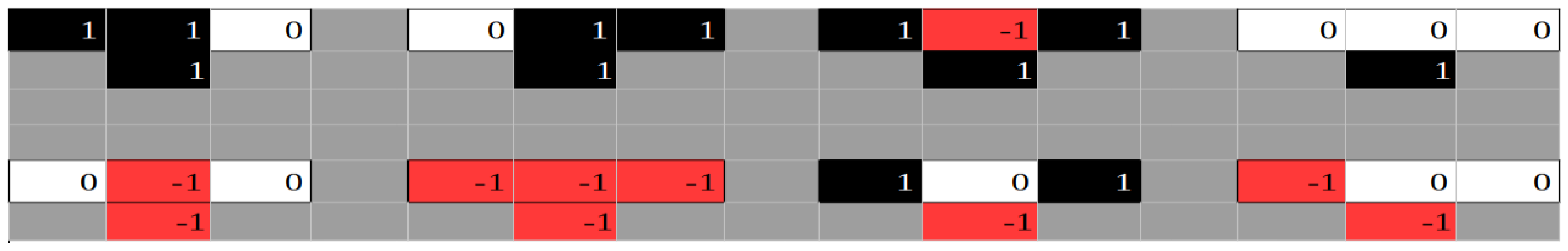
We propose a Boolean Network model with 32 agents. The agents trade only one asset. In each iteration, each agent can be in three different states or positions. Long (1), that is, buying; do nothing, or hold (0), that is, neither buying nor selling; and short (−1), that is, selling. The existing pattern of individual positions gives the configuration of the system at any given point in time.
The dynamical law or the rule for updating the status of agents is synchronous, local, and universal. The status of all agents is updated at the same time, during each iteration. All agents use the same status-updating rules. The rules are local and represent variations of Wolfram’s Cellular Automata rules [
63,
64], in particular Rule 110. Rule 110 is an elementary cellular automaton that describes the status of a cell across several iterations based on the status of its immediate neighbors. The outcomes of this rule are 01101110, which is the binary equivalent of 110.
Our agents rely only on the status of the nearest neighbors to the right and left. An exemplification of one of the rules used here is graphically represented in
Figure 1.
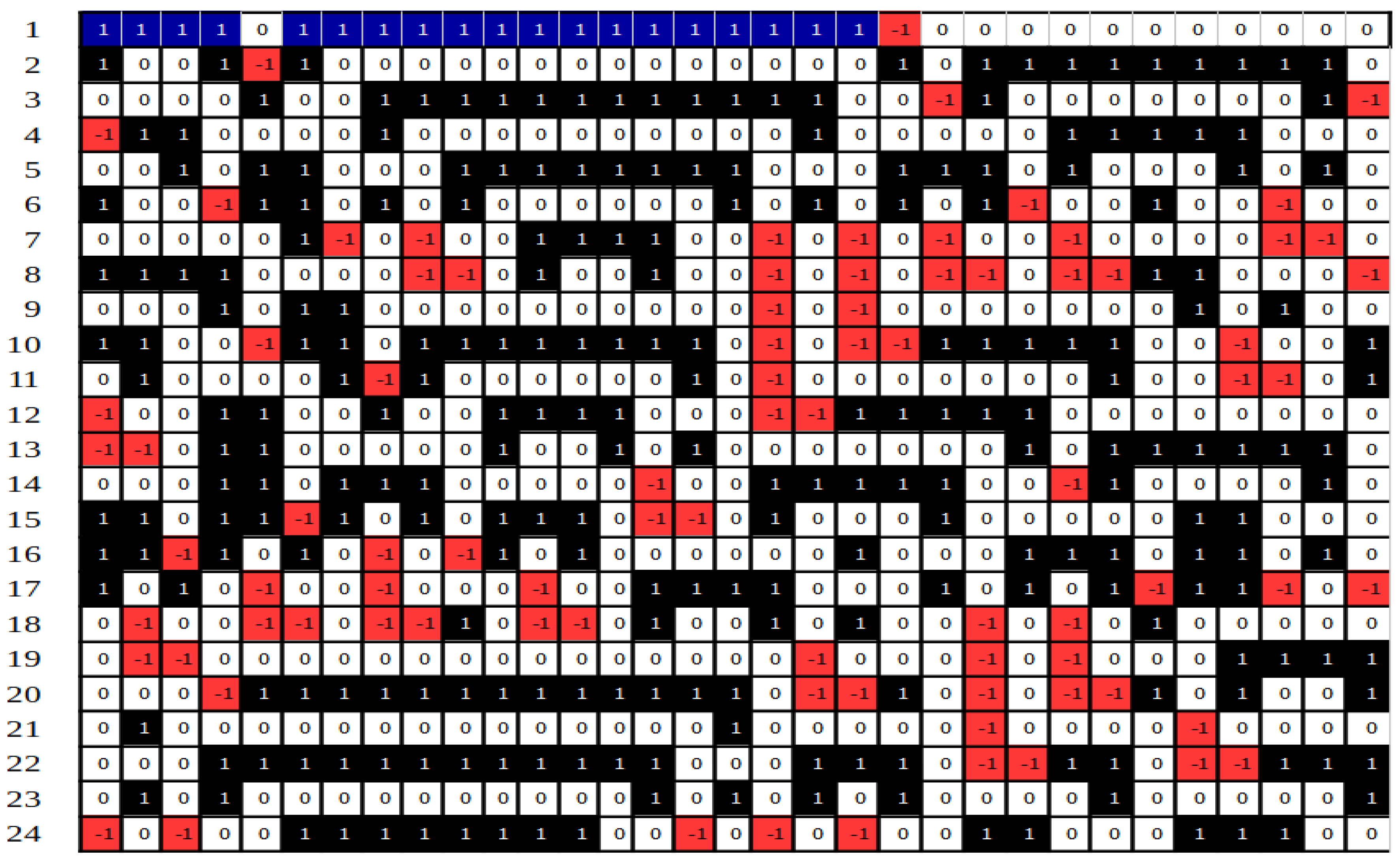
At t = 1, the agents are initialized. We have also experimented with restricting selling at the very beginning, but we found the results were not sensitive to the initial conditions; other things held constant. An example of the emerging pattern of buying, holding, and selling is presented in
Figure 2.
We define the Net Current Position (NCP) at each iteration as the sum of individual positions:
We define the Change in the Net Current Position (t) as the difference between two consecutive Net Current Positions:
We define the Long-to-Hold and Short-to-Hold ratios as:
The price is estimated with the help of three alternative recurrent formulas.
where k
1, k
2, k
3, k
4, k
5, and k
6 are constant parameters.
The choice of formulas and parameters is to a great extent arbitrary. The only constraints are that the price is self-referential and that it represents some function of the number of long and/or short positions and/or of their change. The price represents a recurrent linear transformation that transforms the Nx32 matrix, representing the overall configuration of the system over N iterations, into a Nx1 vector, representing the asset price over N periods.
We also build optional market squeezes into our model. When activated, we constrain the position taken by each agent based on accumulated cash balances. Market squeezes always override the dynamical law.
A short squeeze can be triggered when the cash balance is larger than a critical value parameter that is part of the initial conditions. When a short squeeze occurs, the agent must take a long position, that is, buy in the next iteration, regardless of its neighbors’ positions. This is so because large positive cash balances accumulate as a result of a long-term imbalance between the number of times the agent has been selling as opposed to buying.
If
cash balance (i, t) > cash balance (critical)
then
Position (i, t + 1) = 1
A long squeeze can be triggered when the cash balance is smaller than a critical value parameter that is part of the initial conditions. When a long squeeze occurs, the agent must take a short position, that is, sell in the next iteration, regardless of its neighbors’ positions. This is so because large negative cash balances accumulate as a result of a long-term imbalance between the number of times the agent has been buying as opposed to selling.
If
cash balance (i, t) < cash balance (critical)
then
Position (i, t + 1) = −1
4. Results
We are able, in principle, to generate an arbitrary large number of simulated data series. We can vary the initial conditions of the 32 agents by alternating their initial status and by including and/or excluding either or both long/short strategies for each individual agent. The number of simulated data series obtained over the entire range of possible initial conditions is (332)(264). If we also account for alternating the interaction rule among agents, we obtain a combined number of (356)(264) possible data series. Because we use three different price calculations and allow for a market squeeze, the total becomes (357)(265).
We do not set out to evaluate all possible combinations. Obviously, we cannot realistically perform such an analysis even if we wished to, nor is it necessary. Unlike previous studies, we are not interested in prediction either. As a result, we are not concerned with issues such as the calibration, validation, and the predicted accuracy of our simulation. We are interested in obtaining at least one or more data series that bear close resemblance to real market data.
For the same reason, we are not concerned with the change in dynamics as the number of agents increases. We have tried networks with 64 and even 128 agents without a noticeable change in outcomes. We settled for the 32-agent model simply because the visuals are easier to display and report. Even if the dynamics would change with an increase in the number of agents, that would not affect our conclusions as long as we are able to find and report at least one or more outcomes that match our requirements.
We have chosen five real market data series as a benchmark for comparison purposes. The choice of assets is largely arbitrary. The data covers a period of roughly three recent years of daily observations, as shown in
Table 1. The choice of period and length is driven by the need to have enough observations to draw meaningful statistical inferences and avoid unwieldy and cluttered graphs. We acknowledge that the last three years or so represent quite an interesting period, marred by crises, pandemic, and even war. During periods of relative calm, stock prices are relatively well-mannered and their behavior resembles the much-idealized random walk. It is mostly during periods of turmoil that their behavior starts to display the amazing complexity that is notoriously hard to model. This is when we are able to observe intricate patterns of bubbles and crashes that defy even the most sophisticated stochastic modeling tools. To make our comparisons meaningful, we have settled for a length of 1000 iterations for our computer-generated data.
We notice the visual patterns of most generated data series are very stable with respect to changes in initial conditions. For example, when generating data with P
2(t), we obtain a very distinctive price profile that is extremely resilient over a vast range of initial conditions (
Figure 3). Unlike processes that are extremely sensitive to changes in initial conditions, ours are hinting at the presence of a critical phase transition poised at the edge of chaos [
65,
66,
67]. It is not at all surprising that our model, which is essentially a Cellular Automata, will reveal attractors and basins of attractions [
68,
69,
70,
71,
72]. For example, the Garden of Eden in
Figure 3 lasts for about 200 iterations, after which the series settles into an easily recognizable pattern [
73,
74,
75].
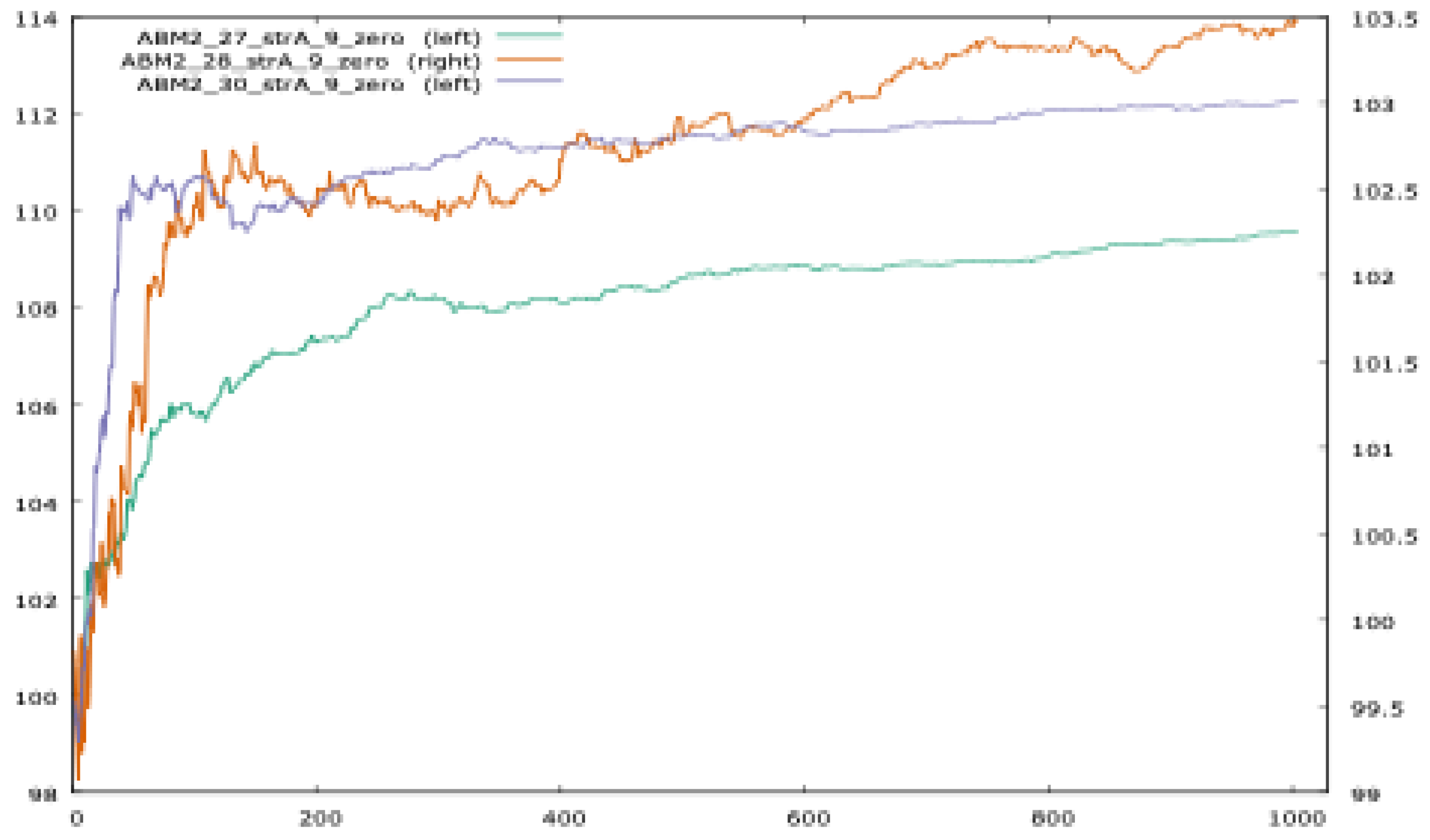
The more versatile data series are generated with P
3(t). We notice the homeostatic signature of a process poised at the edge of chaos. Our simulated data has outstanding mimetic properties, embracing a wide range of patterns, from the very simple linear, to harmonic oscillations, to the patterns that mimic random walks. Here, we show only the ones that look similar to real market data (
Figure 4).
This result is emblematic of the research around the universality of computing in cellular automata [
63,
76,
77,
78].
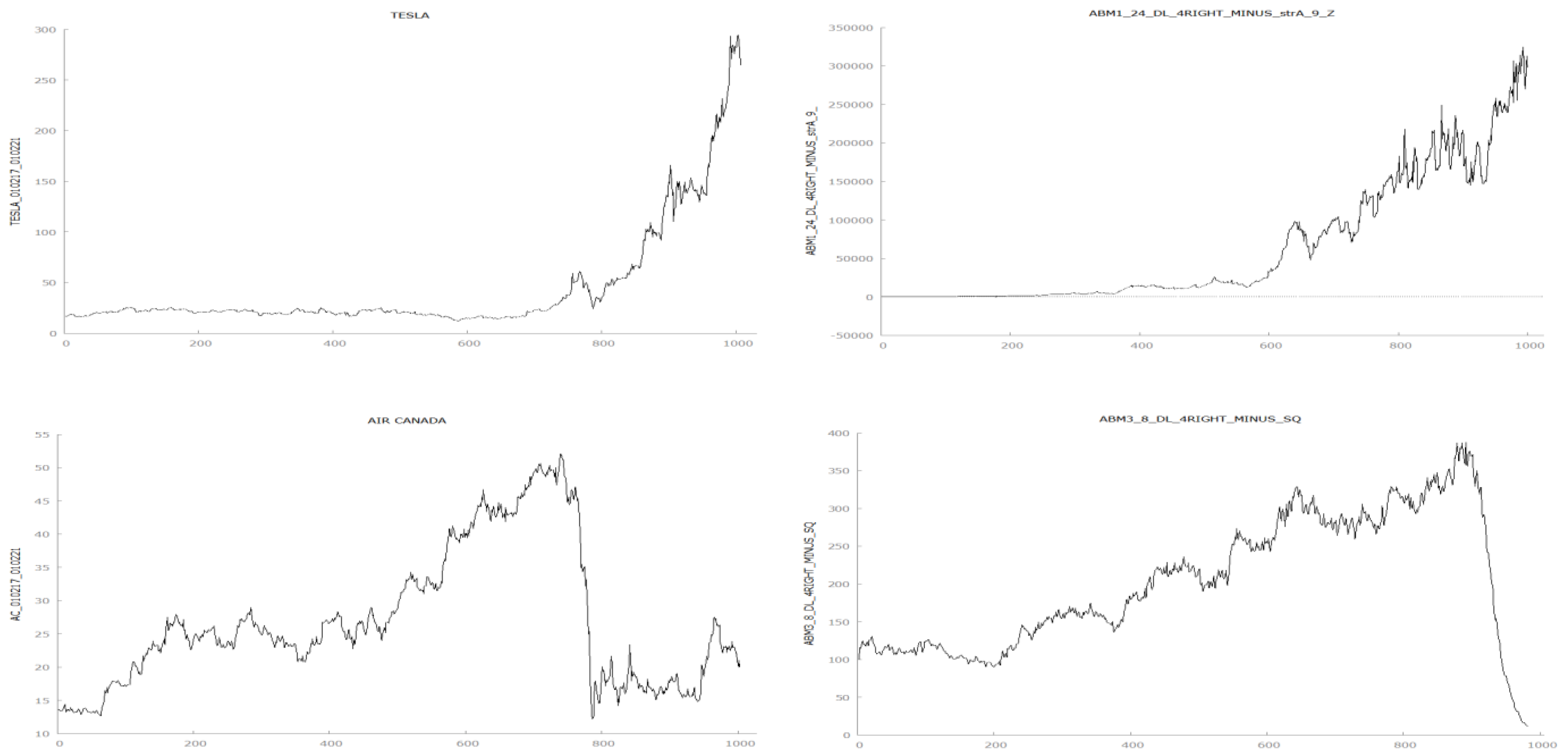
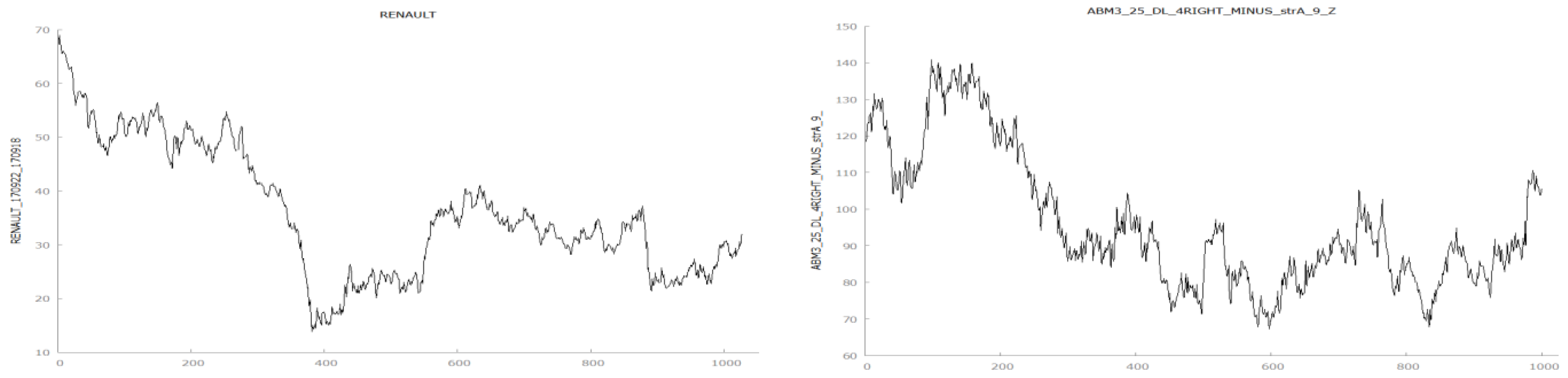
Since an exhaustive evaluation of all computer-generated data series is not tenable, we have generated a small sub-sample of simulation data and identified several of them that exhibit patterns similar to those of real data. Of a sub-sample of 600 generated data series, we estimate that roughly 7% of them, or 42 data series, look extremely realistic.
A side-by-side cursory analysis of real stock prices and ABM-generated series reveal how strikingly similar they look. Upon visual inspection, it is almost impossible to tell the difference among them. There is no discernible visual clue to help telling apart real from generated data (
Figure 5).
We run unit root tests for all data series, real and simulated. The Augmented Dickey-Fuller test coefficients are not statistically significant in virtually all instances, hence, as expected, we fail to reject the null hypothesis of mean stationarity for both real and simulated data.
We also perform a Wald-Wolfowitz runs test to determine if indeed the data is occurring at random and if there are any patterns. The null hypothesis assumes the data is generated by a random process. In the case of real data, we fail to reject the null hypothesis in all five instances (we only report the results for three of them).
The results are split in the case of realistically looking simulated price series. In several instances, the results fail to reject the null hypothesis, whereas in others they appear to reveal autocorrelation patterns in the data (
Table 2). We do not report all results, we only show a small fraction of them. We consider it is enough to show there is at least one or more simulated series that have similar properties to those of real market prices.
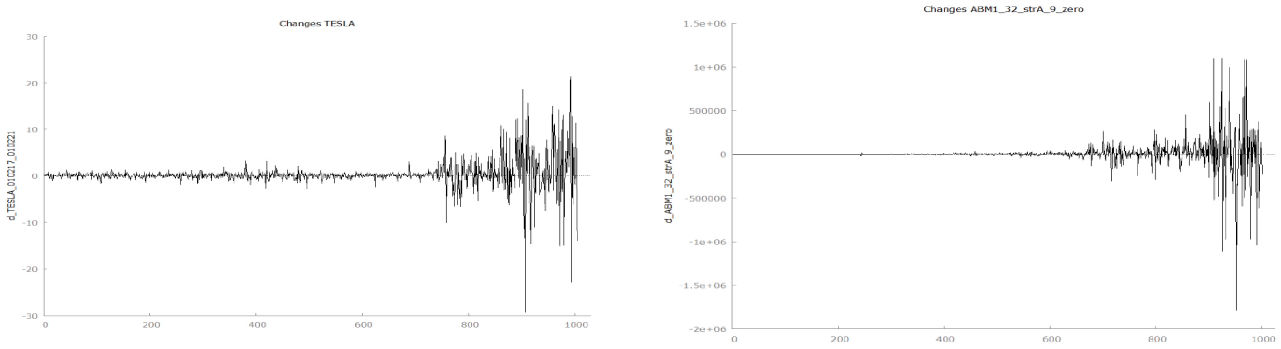
The first-order differences for all data, real and simulated, appear mean-stationary, but not variance and covariance stationary (
Figure 6 and
Figure 7).
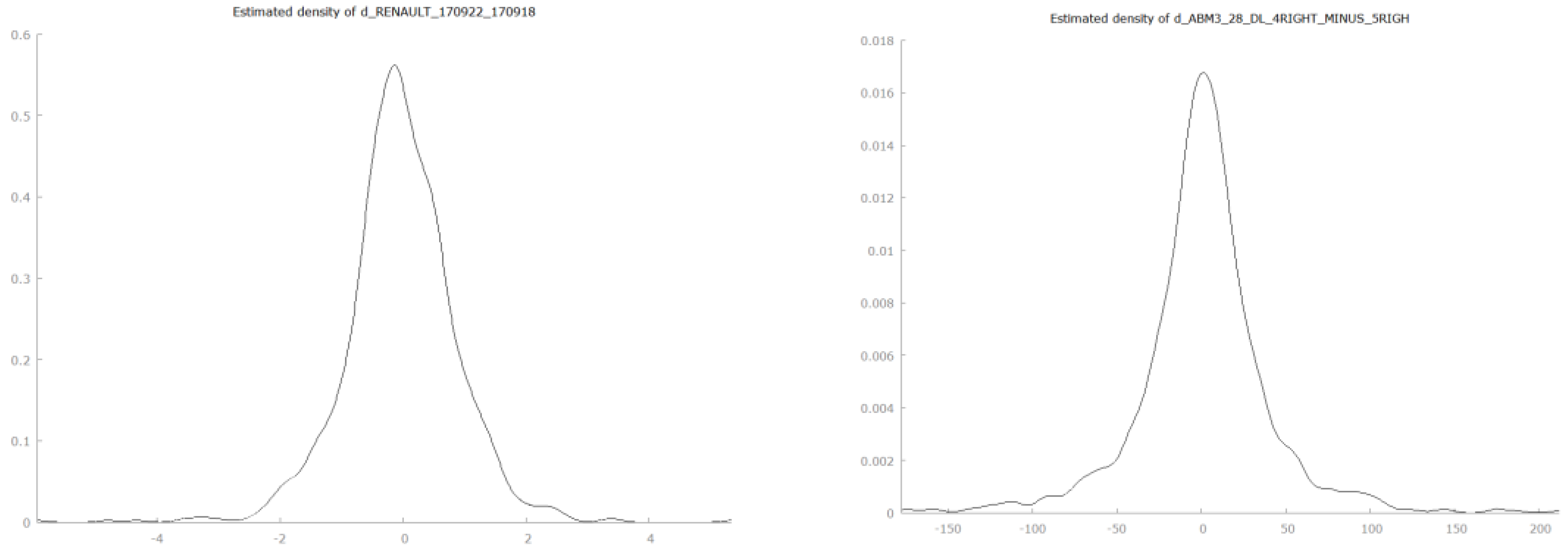
Not all first-order differences have similar distribution characteristics. The ones who look just like real data have first-order distributions that are undistinguishable from those of real data. Also as expected, none of these distributions are normal. Tests for normality have been performed, but they are not reported here. We have decided to run pairwise non-parametric tests instead, and failed to reject the null hypothesis in all but six instances. We do not report all results, however. For example, first-order differences of Renault’s stock price are compared to those of ABM3_28_DL_4RIGHT_MINUS_5RIGHT_Z. The Wilcoxon signed-rank test (H0: the median difference is zero) returns a z = 1.41216 and a two-tailed
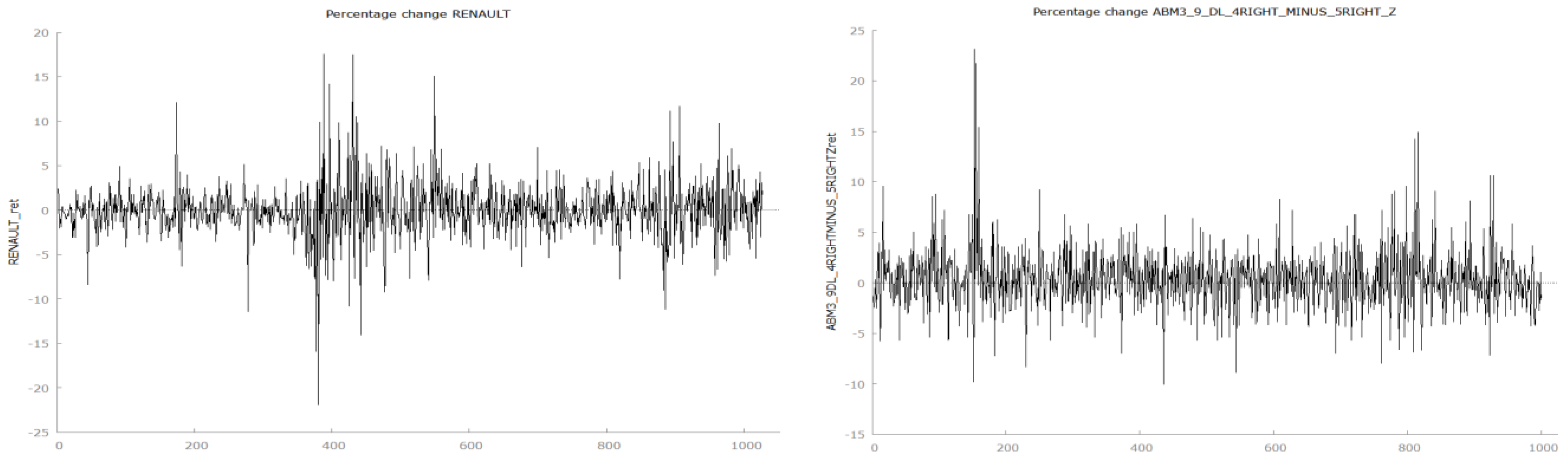
p-value of 0.157904, thus failing to reject the null hypothesis that the two distributions share the same location. The visual inspection of return time series shows the familiar pattern of volatility clustering and suggests the series are not variance stationary (
Figure 8).
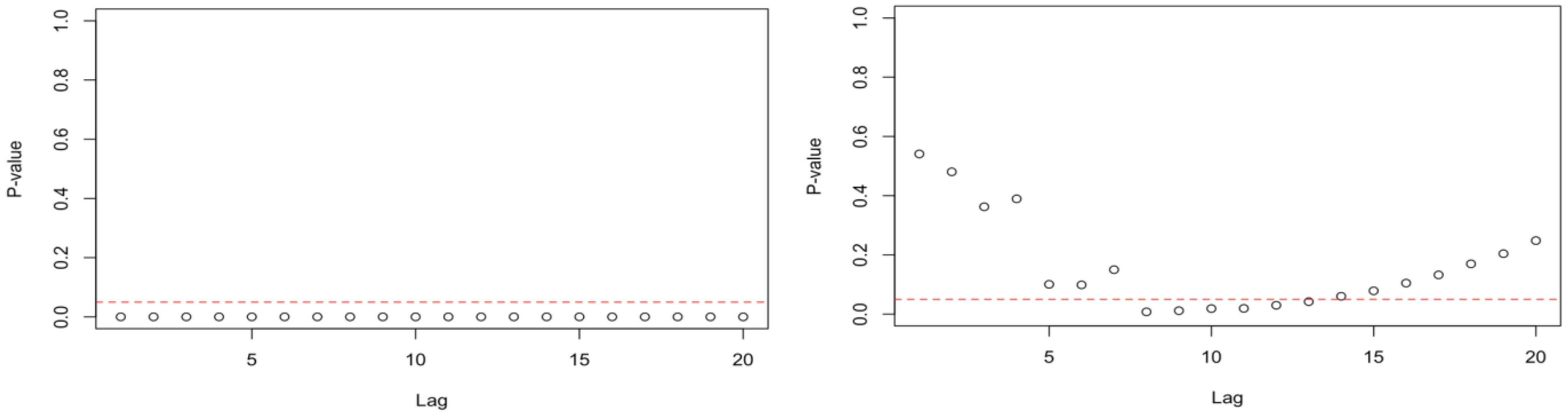
To determine whether Auto-Regressive Conditional Heteroskedasticity (ARCH) is present, we run the McLeod-Li test with a default of twenty lags. The null hypothesis is that of no heteroskedasticity.
In the case of real time series, the tests reject the null at all lags except for Renault, where we reject the null only for the lags 8 to 13 (
Figure 9). In the case of simulated time series, we find that all 42 series that bear close resemblance to real data exhibit the same pattern of heteroskedasticity.
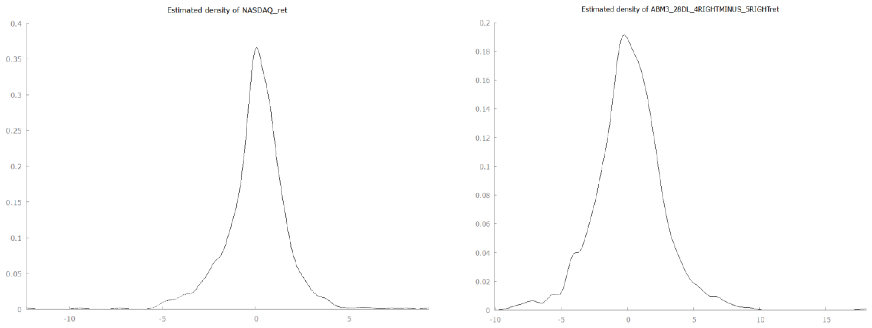
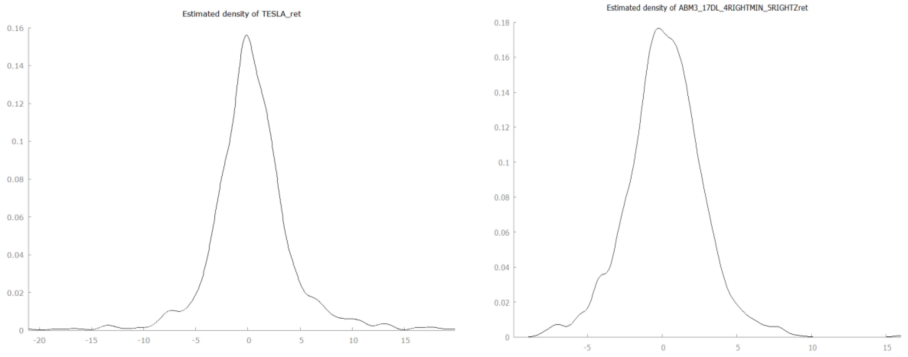
The return distributions show the familiar leptokurtic shape for both real market and simulated data (
Figure 10). As expected, return distributions are not normal. We run normality tests, but we do not report the results here. Excess kurtosis ranges from 4.92 for Tesla to 16.42 for Carnival and from 1.17 to 283 for the simulated data. The median excess kurtosis for simulated return distributions is 2.89. Clearly, there is a wider variability in the shape of simulated distributions, but all 42 real-data look-alikes are leptokurtic. Yet again, our real data benchmark is made of only five stocks.
We pair real return distributions with simulated return data and perform nonparametric difference tests. Due to the extremely large number of procedures, we do not report the results here. Most tests results, however, fail to reject the null hypothesis. This makes for a truly remarkable result.
For example, we compare the distributions of returns between NASDAQ and the simulated series ABM3_17_DL_4RIGHT_MINUS_5RIGHT_Z. The Wilcoxon Signed-Ranked Test returns a z = −0.154019 with a corresponding two-tailed p-value = 0.877594. Hence, we fail to reject the null hypothesis that the two distributions share the same location.
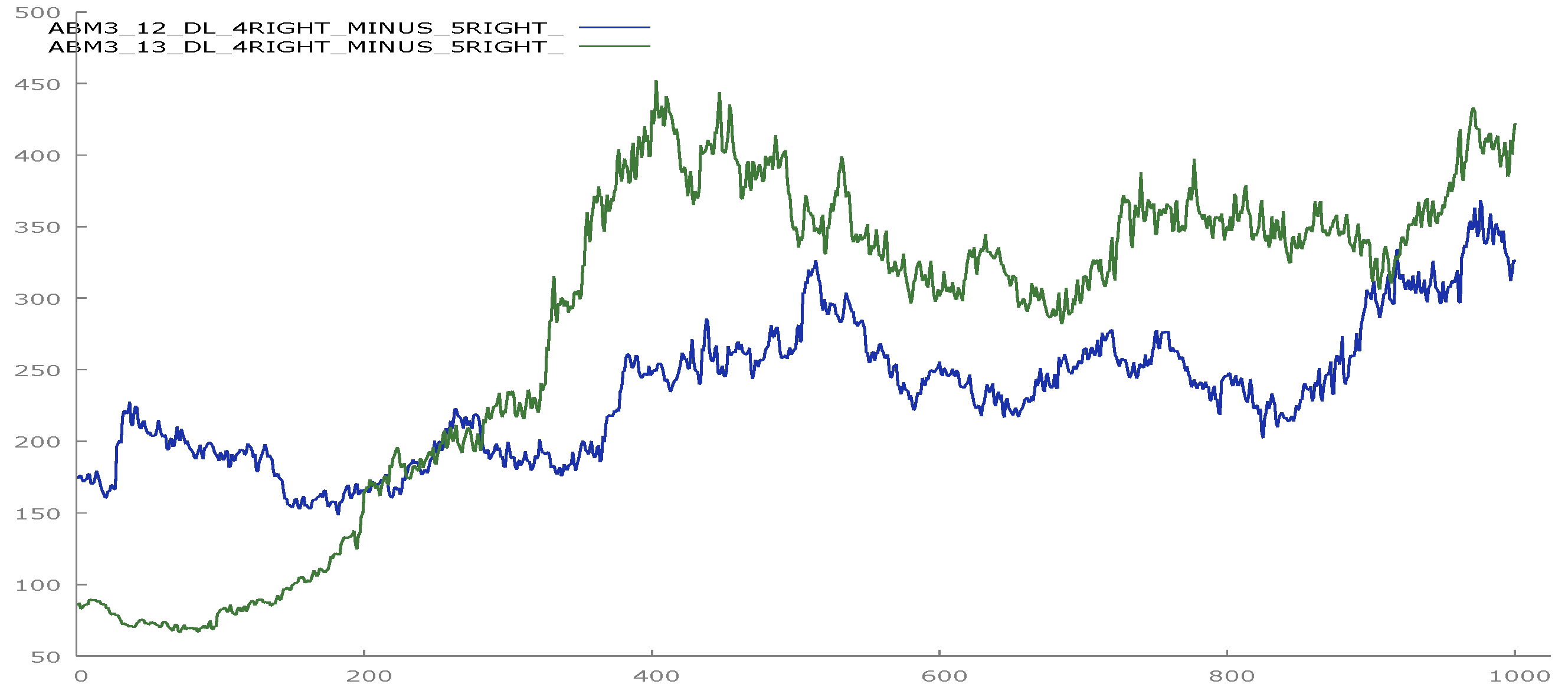
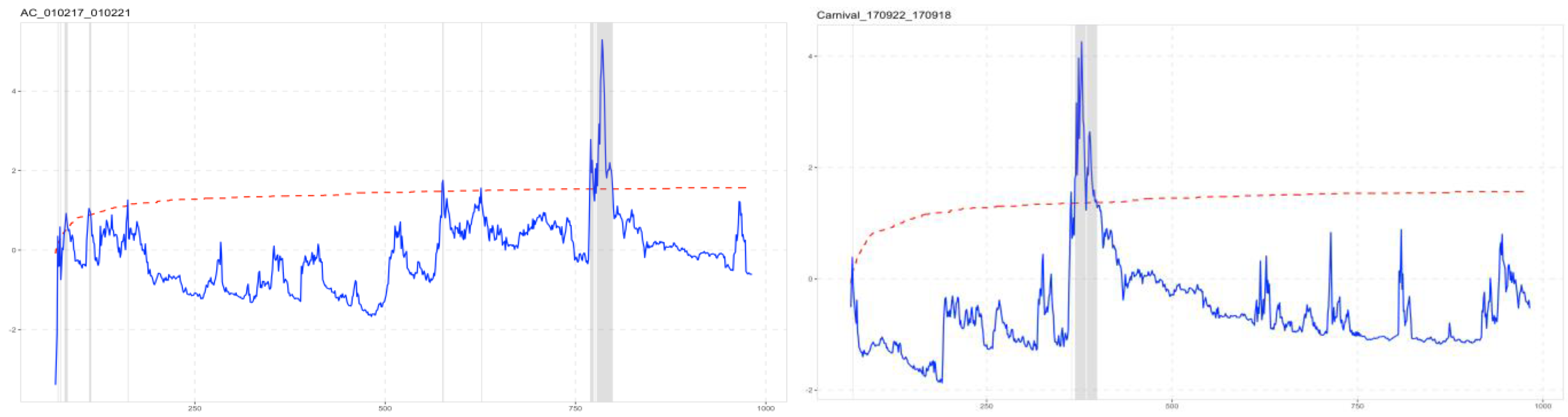
To detect the presence of bubbles we run a test for the occurrence of explosive time series. This relatively novel test [
79] has several variations depending on how the rolling window is iterated: Supremo Augmented Dickey-Fuller (SADF); Generalized Supremo Augmented Dickey-Fuller (GSADF); or Backwards Supremo Augmented Dickey-Fuller (BSADF). In essence, all variations test the coefficient of the lagged dependent. In the case of the regular ADF, the null is a coefficient of zero, that is, the presence of a unit root. The alternative is a negative coefficient, which suggests mean stationarity. In the case of the explosive time series test, the alternative is a positive coefficient, suggesting an exponential progression.
The results of the tests performed in R plot the statistic against time and against the level of significance. The iterations during which the statistic becomes significant are timestamped for an easy visual identification and interpretation (
Figure 11). We detect the presence of bubbles in all but one of the real data series. The only one not showing the presence of explosive time series is NASDAQ.
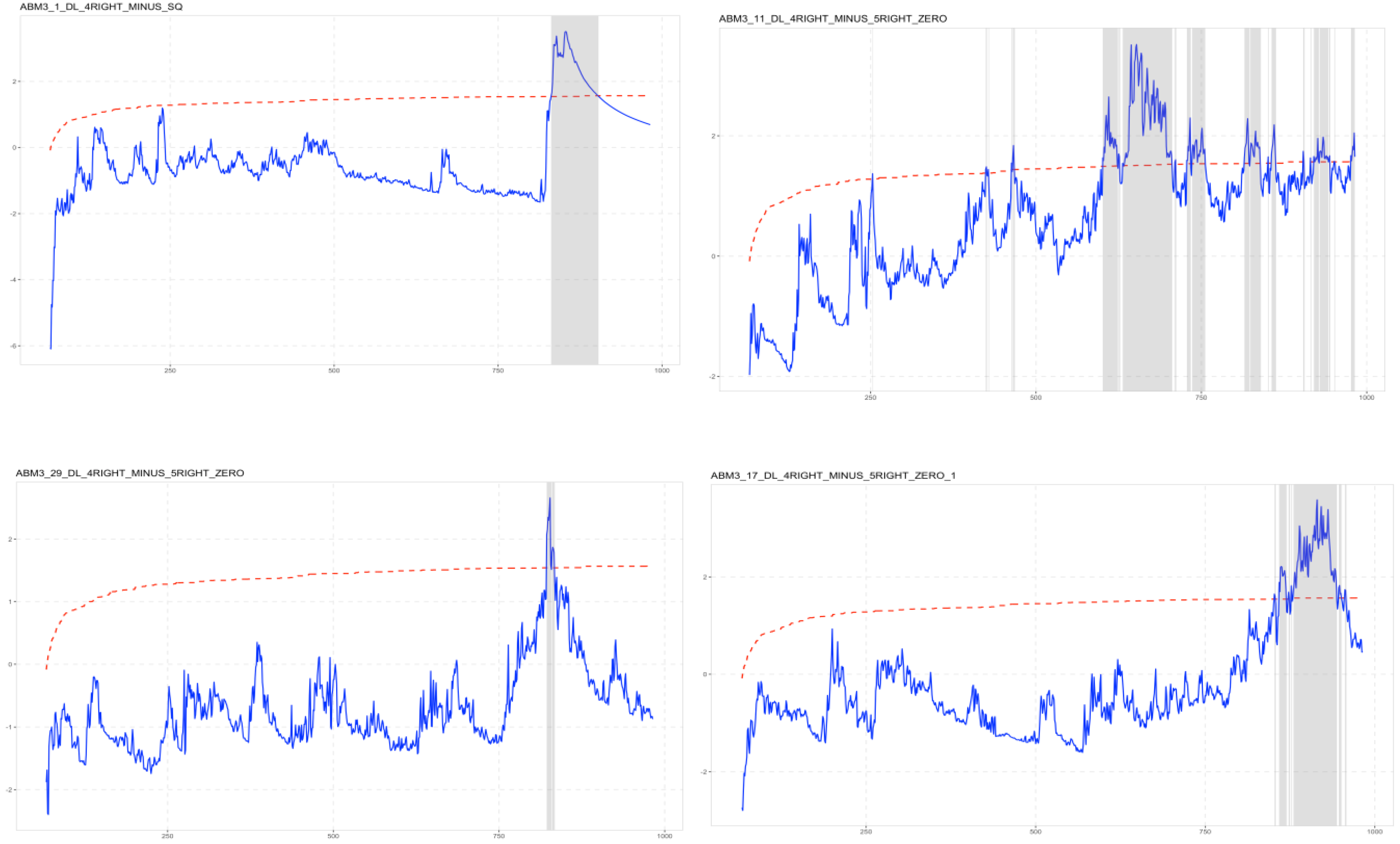
Of the simulated time series, 24 of the 42 who bear close resemblance to real data show a very similar pattern of bubbles. Yet again, they are virtually indistinguishable from real market data. Here, to make a comparison, we show only four results, chosen arbitrarily (
Figure 12).
Next, we run a GARCH model to compare and contrast the return characteristics of our various data series. We report only the case of TESLA and ABM1_32_strA_9_zero (
Table 3). The results are consistent with previous findings. Both GARCH (1) and ARCH (1) coefficients are surprisingly similar in magnitude. Moreover, the statistical significance of the coefficients is comparable. It would be indeed very difficult to tell apart the real versus simulated return series based on the above results.
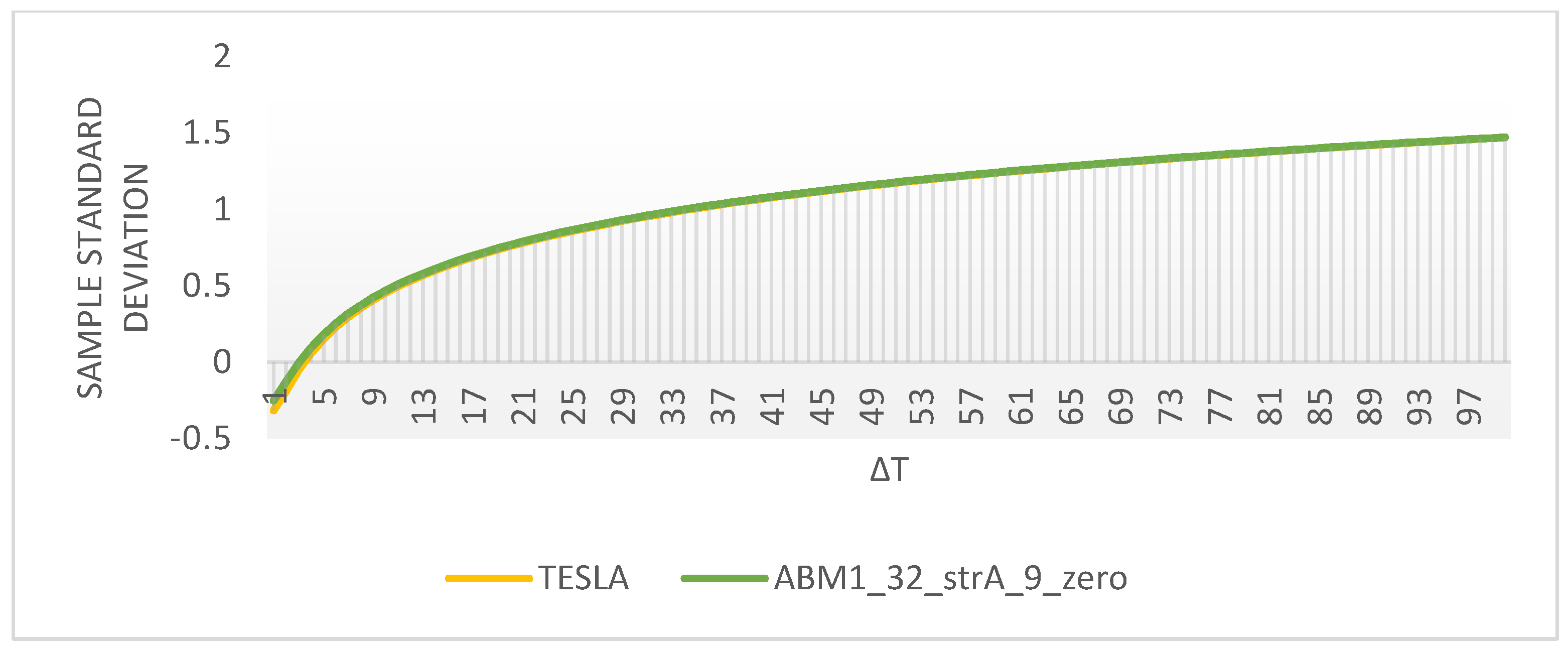
Last but not least, we conduct a comparative spectral analysis in the spirit of [
53]. Yet again, for the sake of brevity, we only report the results of only one comparison involving TESLA and ABM1_32_strA_9_zero returns.
The double log of the standard deviations of returns at different sampling intervals looks almost indistinguishable (
Figure 13).
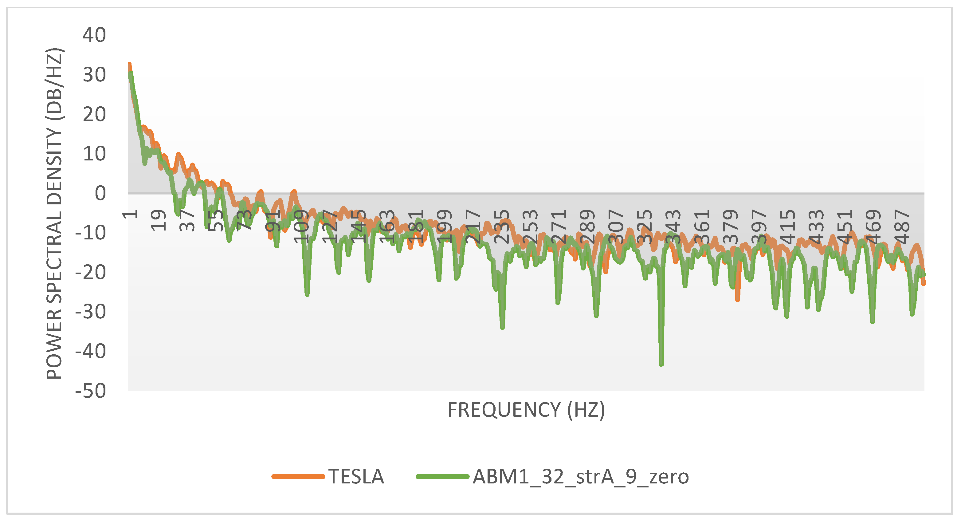
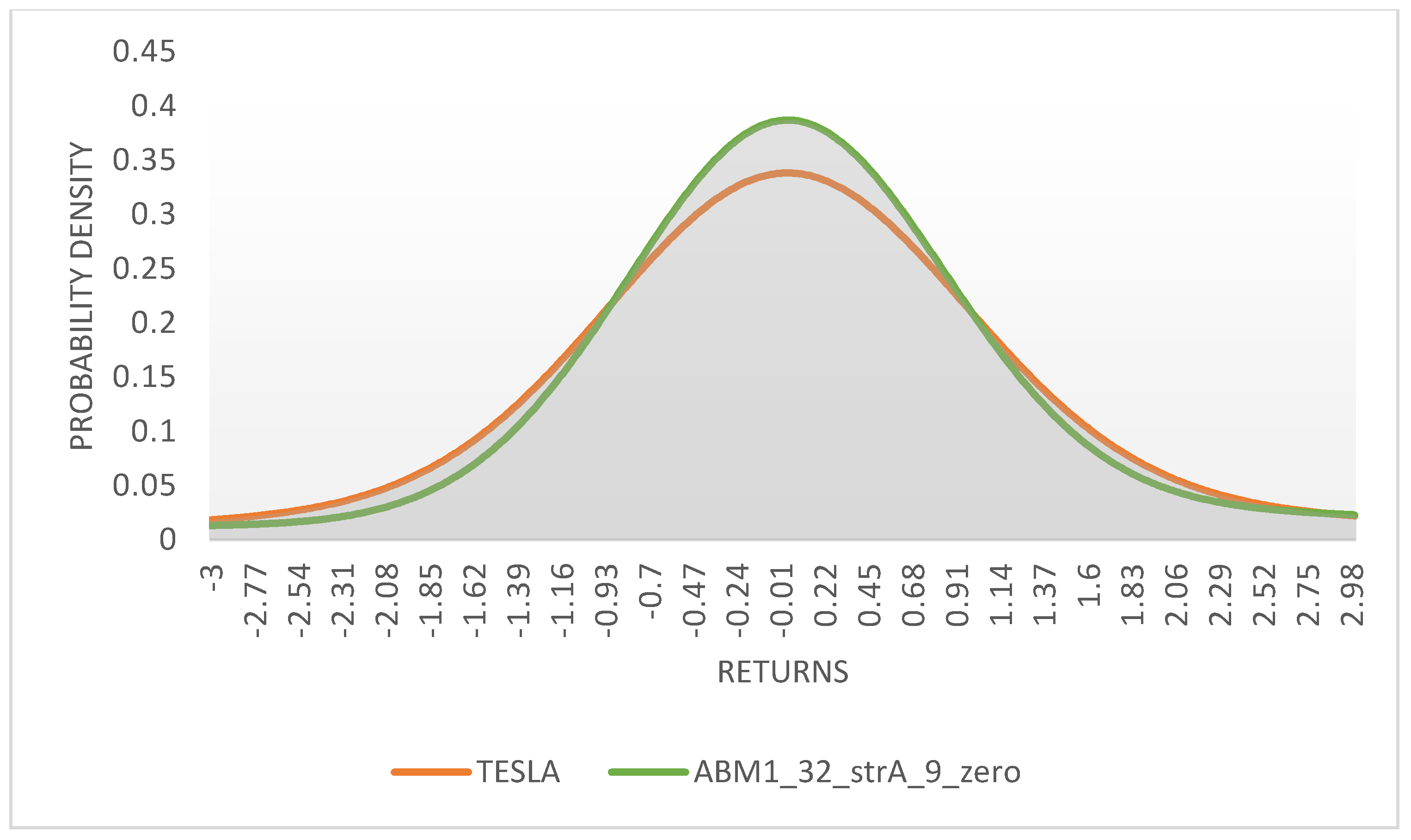
The power spectral density of the signals is presented in
Figure 14, and the kernel density estimates of the marginal distribution of returns at ∆t = 1 are shown in
Figure 15.
Both Power Spectral Densities (PSD) and Probability Density Functions (PDF) look very similar, reinforcing our earlier results. The marginal PDFs describe the two series under the assumption of stochastic processes, and this brings to the fore a deeper philosophical dilemma.
We know that both our model and real markets are essentially deterministic systems. They are neither random, nor stochastic. The use of stochastic modeling is at best the manifestation of a substitution bias. Stochastic models appear to be one of the very few tools available for getting a grip on the dynamic of social and economic systems. As explained in this paper, they also preserve the illusion of some sort of predictive and/or normative management. Using more advanced statistical tools above and beyond ARCH and GARCH is not adding much more to what we already know; it is, however, reinforcing the misconception that the nature of the market dynamic is stochastic.
5. Discussion and Implications
We have generated a sample of agent-based financial prices and compared it to a small sample of real market-data. In terms of inference with commonly used statistical tools, our simulation processes look extremely realistic.
Our goal was to show at least one or more simulated data look undistinguishable from real data when viewed from the lens of statistical inference. We did not proceed with an exhaustive analysis of all simulated data for reasons that are obvious. Of a subsample of 600 simulated data series, 42 look very similar to real data, and 24 passed all statistical tests. We suspect, however, the possible number of deep-fake prices to be much larger.
To the extent that statistical tools such as hypothesis tests ubiquitously rely on the assumption that the underlying data generating process is stochastic, these results emphasize that inference regarding features of financial markets is extremely sensitive to this assumption. Indeed, when applied to data generated from an arbitrary deterministic process, we obtain nearly identical inference from these tools as when applied to real-world stock price data.
The model presented in this paper is much simpler and generates data that bears an uncanny resemblance to reality. We cannot emphasize enough the relative arbitrariness of initial conditions and interaction rules.
We cycle among initial conditions/parameters that are more or less arbitrarily chosen, without any pretense of functional realism. Yet, this model is generating outcomes that look very similar to real outcomes. The model is able to do so, not necessarily because it reflects the functional characteristics of reality, but because it is computationally equivalent to reality. It has a similar level of complexity but without all the functional properties at the ground level.
In some sense, our generated data series are deepfakes. A deepfake is an image or recording that has been manipulated to misrepresent someone as doing something that was not actually done. Our model can be tweaked into doing something that is not real but looks real. Our model does not reflect the real world; rather, it can impersonate real world outcomes. This nuance is crucial to understanding our point.
We contend the implications of our results pertain to predictability, investor behavior, and regulation of financial markets.
Most of our deep-fake price series were generated based on variations of Wolfram’s Rule 110 [
64,
80]. Wolfram claims Rule 110 is in fact an instance of universal computation. If so, that could explain the wide range of behavior obtained: from linear to harmonic to random and to complex. It is very likely our deep-fake price series belong to Wolfram’s Class Four, the class of phase-transition processes poised at the edge of chaos. Although we are not concerned with prediction, our findings add another twist to the quest for predictability.
Just like random walks, critical processes deny us the ability to make predictions, but for different reasons. Under a random walk, prediction is in principle valid but not reliable. It means investors still have rational expectations. However, if stock prices are emergent from a universal critical process, prediction is not even possible in principle. There is no method for finding future outcomes faster than in real time. Critical universal processes are undecidable and computationally irreducible [
76,
81].
Unlike other agent-based models, we do not endow our agents with either rational expectations or cognitive distortions. Our agents are not expected to “behave” realistically, and we are not seeking to calibrate or validate our inputs, because realism and prediction are not the objectives of our exercise.
This deceptive simplicity of underlying rules is a nod to the Principle of Computational Equivalence, and we hope our findings will settle once and for all the ongoing debate around the impact of investor behavior on stock prices.
That economic agents exhibit cognitive distortions and do not follow the axioms of rationality is no doubt a momentous advance in the area of Economics and Finance. However, although there are countless implications following from here, it might not matter so much from the perspective of stock prices. Based on our findings, we contend that rational agents do not necessarily lead to random walks, and biased investors do not necessarily generate the bubbles, crashes, and anomalies documented by econometric studies. Rationality or lack thereof makes sense only in the presence of sentient agents making investment choices under risk. Our model is purely deterministic and has no stochastic component whatsoever. There is no uncertainty or risk present; hence, it makes no sense to refer to the behavior of the agents as either rational or irrational. To put it bluntly, investor behavior as we understand it might not matter at all.
If such simple rules are sufficient to generate realistic data series, deciding whether economic agents are rational or biased does not add anything to our understanding of the emerging market behavior. Our simple cellular automata world is capable of generating a level of complexity equivalent to that of the real world in the absence of moral agency. That real-life individuals are driven by a sense of purpose and agency, capable of planning and strategizing, experiencing emotions, desires, and engaging in sophisticated abstract thinking and complex behavior, might be merely an incidental aspect and not a defining characteristic.
Many other scholars who pursued agent-based models felt compelled to posit as complex an individual behavior as possible to explain the emerging complexity of financial markets. There is an implicit belief here that the more complex the underlying behavior of the individual agents, the more complex the behavior of the overall market. But the Principle of Computational Equivalence sets an upper limit to the level of complexity achievable by any type of process.
It means the simplest conceivable interaction bearing a very vague resemblance to reality, like the one we propose here, is capable of generating an overall system behavior quickly reaching the upper limit of achievable complexity. From a purely computational perspective, some of the cellular automata rules we employ here do not merely approximate but are computationally equivalent to the richness and sophistication of human interaction. It follows that our models should not be unnecessarily burdened by elaborate assumptions trying to replicate the intricacies of human behavior. The more unsettling observation is that the actions of moral agents are not even a requirement.
Finally, our findings have consequences for the regulation of financial markets. There is a growing body of evidence that finds no compelling link between the implementation of regulation and the achievement of desired policy objectives over the long run. Most of economic crises and market crashes have been attributed to insufficient regulation or lack thereof. Every crisis has prompted a regulatory overhaul that did little to prevent the next crash. The Sarbanes-Oxley Act passed in the wake of the Enron debacle was ineffectual in avoiding the subprime meltdown of 2007. At times some of the intended short-term objectives are attained, but at a tremendous long-term cost incurred somewhere else [
82,
83,
84,
85].
To the extent to which regulation is merely impacting the inputs, that is, the initial conditions of the market system, it is likely their effect will be negligible. We have shown how resilient the behavior pattern of our system is to changes in initial conditions. In the long run, the market will revert towards the same attractors. To the extent to which regulation is providing incentives or punishments that change how investors interact, the outcome will be undecidable as discussed earlier. This explains why regulators always appear to blunder and why regulation is perpetually insufficient or inadequate.
6. Concluding Remarks
The main contribution of this paper is the most parsimonious financial market agent-based model to date. It is a cellular automaton using deceptively simple rules, capable of generating stock price data series virtually indistinguishable from real market data. We do not endow our agents with rational expectations and foresight. nor do we allow cognitive distortions such as herding or overreaction.
Although there is no underlying stochastic process at work and no randomness built into our inputs, conventional statistical tools applied to simulated data yield inferences on “financial market features” that are commonly found with stock price data. Specifically, the arbitrary deterministic processes display characteristics similar to real stock prices, such as lack of stationarity, volatility clustering, return distributions with fat tails, and bubbles and crashes. Our dynamic law used to update the status of our agents represents variations of Wolfram’s Rule 110, and we contend at least some of our processes possibly belong to Wolfram’s Class Four of systems poised at the edge of chaos.
We also believe that for too long economists have been and continue to be hoodwinked by the complexity, richness, and eccentricities of individual human behavior. They assume that the more complex the decision-making process of individual agents, the more complex the resulting market price behavior. In a one-to-one relationship, rationality is believed to lead to random walks, whereas cognitive distortions are held responsible for the price anomalies we observe in the real market. But the link showing how individual rational and/or irrational behavior gets aggregated into market prices has been conspicuously missing.
Our model is not an attempt at reflecting reality but at impersonating it. The model is able to do so, not necessarily because it reflects some functional characteristics of reality, but because it is computationally equivalent to reality. It has a similar degree of complexity but without all the functional properties at the ground level. We show here that the complexity of the real market data has much simpler roots than the quirks of investor behavior. The richness and intricacies of individual behavior certainly add local color, but they appear more like epiphenomena rather than necessary causes. If we replace this complex individual behavior with a simple cellular automaton, we obtain a process of equivalent complexity but without the histrionics. All that is required is feedback and rules based on simple local interaction. No moral agency required.
Another implication pertains to prediction and the regulation of financial markets. To the extent to which our process is critical, that is, poised at the edge of chaos, prediction is denied by undecidability and computational irreducibility. It also means that regulators and policymakers will always be surprised by the unintended consequences of their decisions.
Doling out rewards and punishments to investors might or might not produce results as intended. Ex-ante regulation and policies always look foolproof. Ex-post, however, it will always be obvious why they failed and what should have been done in the first place. From a historical perspective, however, the regulation of financial markets appears more like a tortuous progression of hit-or-misses, rather than thoughtful, purposeful design.


