


Quantitative Analysis of Mixed Minerals with Finite Phase Using Thermal Infrared Hyperspectral Technology
 , ,
, ,
Abstract
:1. Introduction
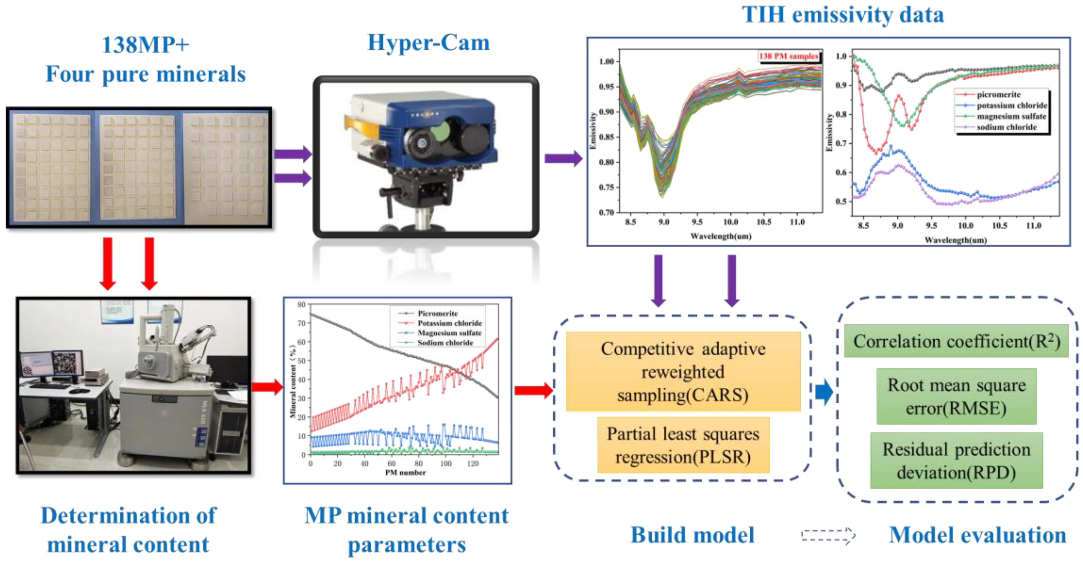
2. Technical Route
3. MP Samples Preparation and TIH Data Acquisition
3.1. MP Sample Preparation
3.1.1. MP Samples
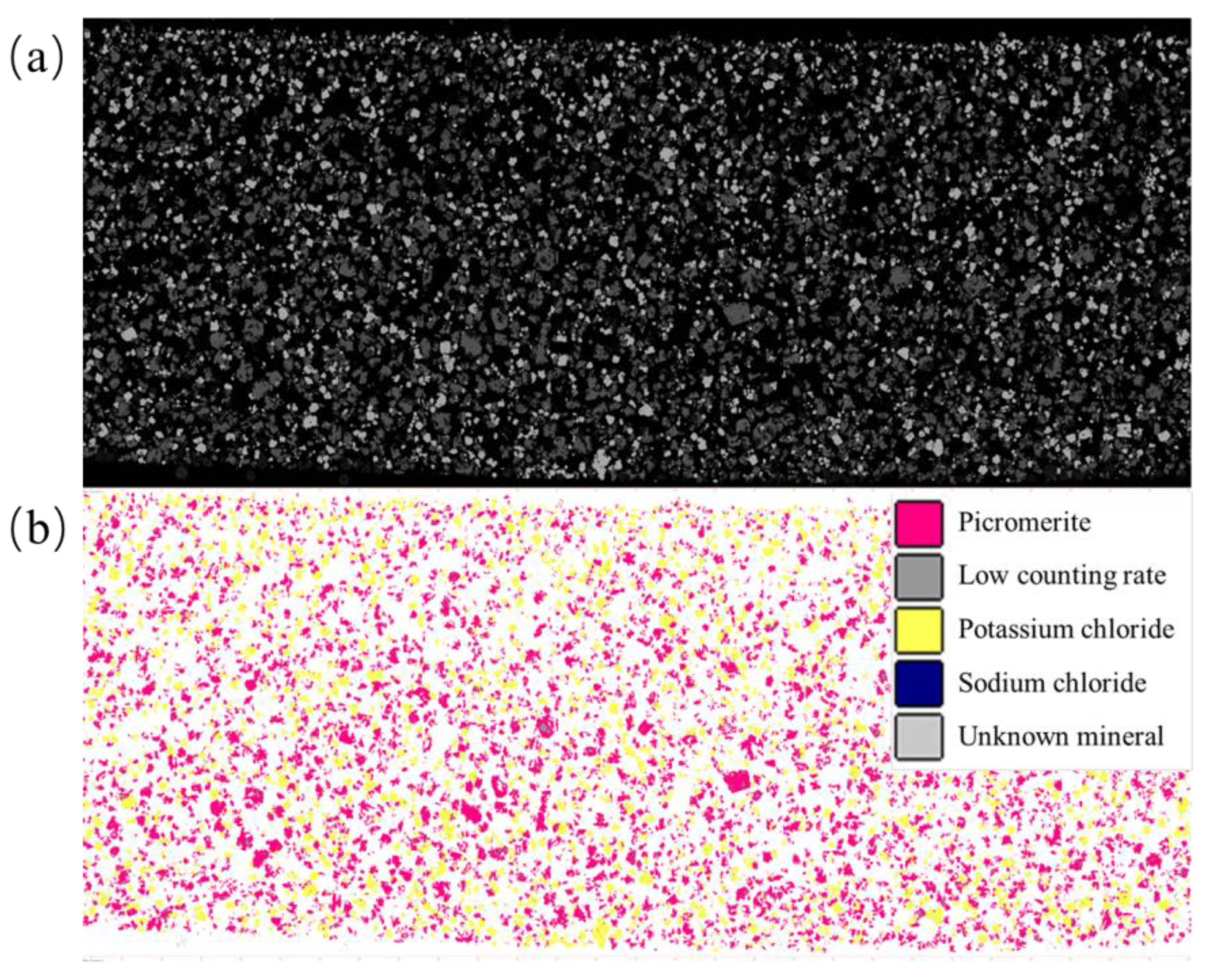
3.1.2. Mineral Facies Analysis
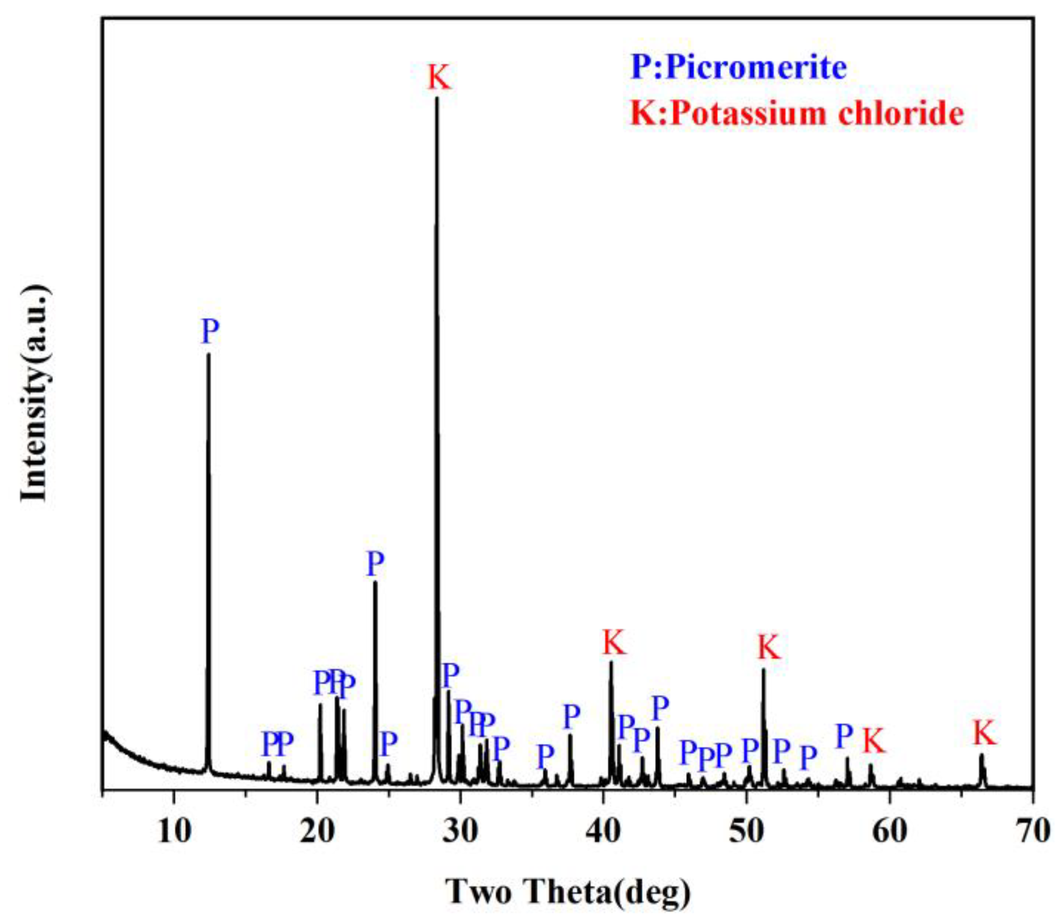
3.1.3. Mineral Composition of MP Samples
3.1.4. Samples Library of MP
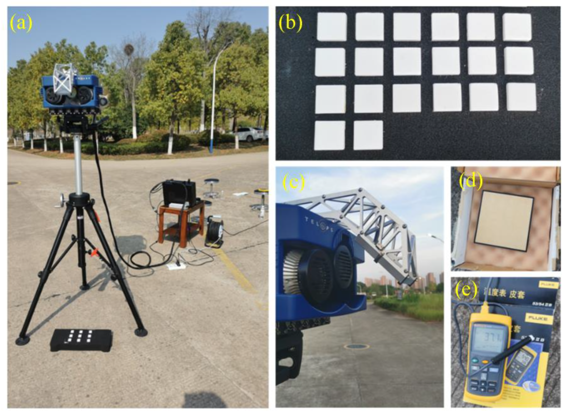
3.2. TIH Data Acquisition
3.2.1. Standardized Processing of MP Samples
3.2.2. Hyperspectral Imaging System and Image Acquisition
3.3. TIH Data Processing
3.3.1. Emissivity Inversion
3.3.2. Data Quality Evaluation by Temperature
4. Methods
4.1. Prediction Model
4.2. Model Evaluation
5. Experiments and Results
5.1. Model Establishment for MP Prediction
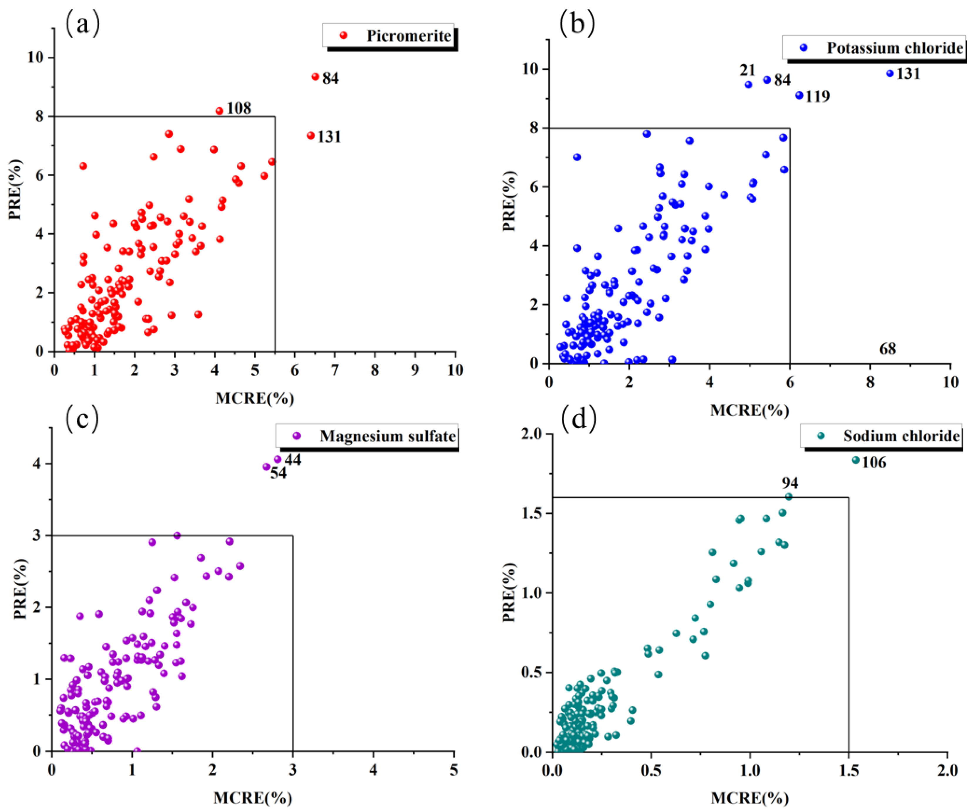
5.1.1. Outlier Detection
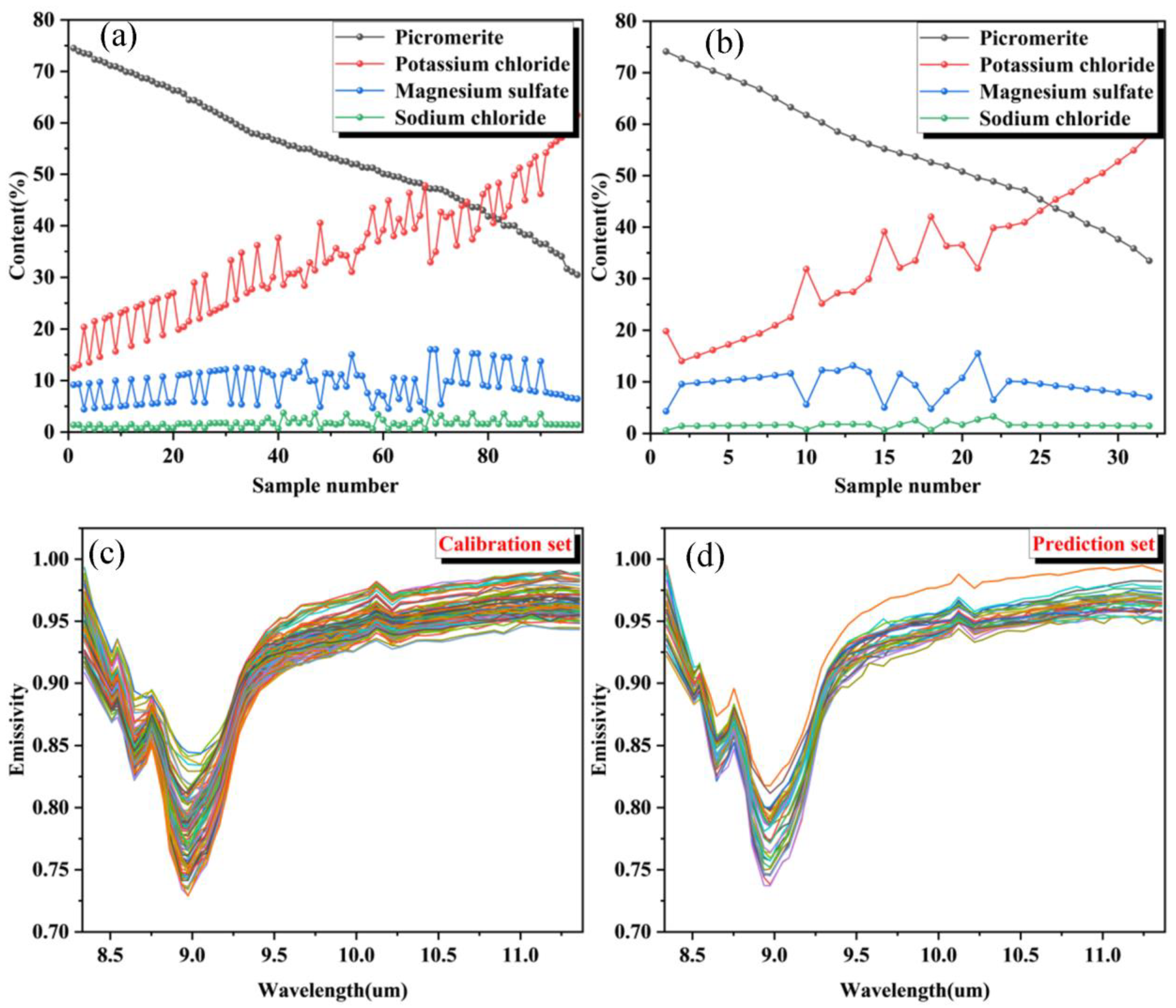
5.1.2. Calibration Set and Prediction Set
5.2. MP Content Prediction
5.3. Sensitive Bands Selection of Pure Mineral
6. Conclusions
- (1)
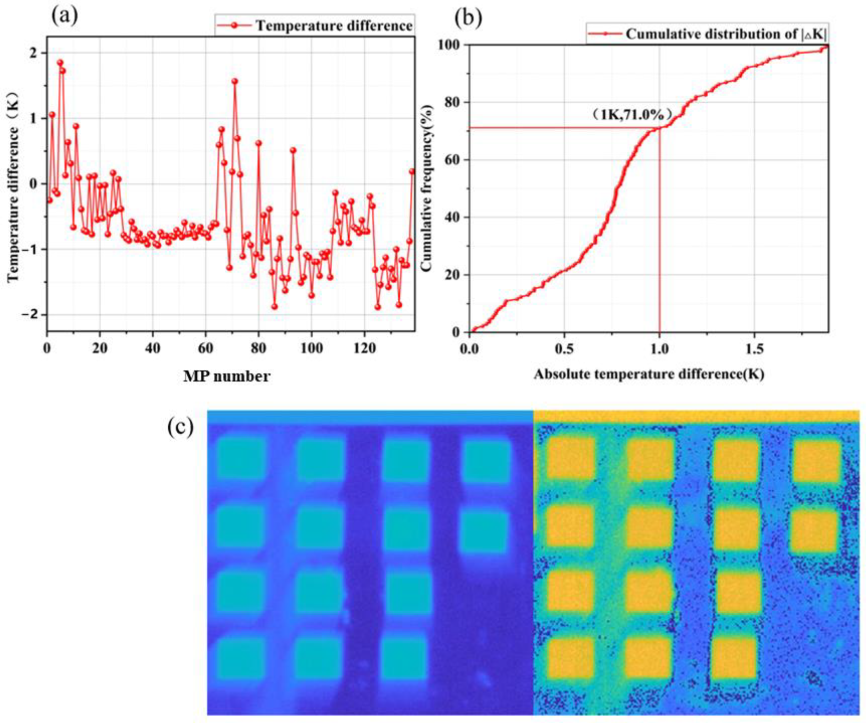
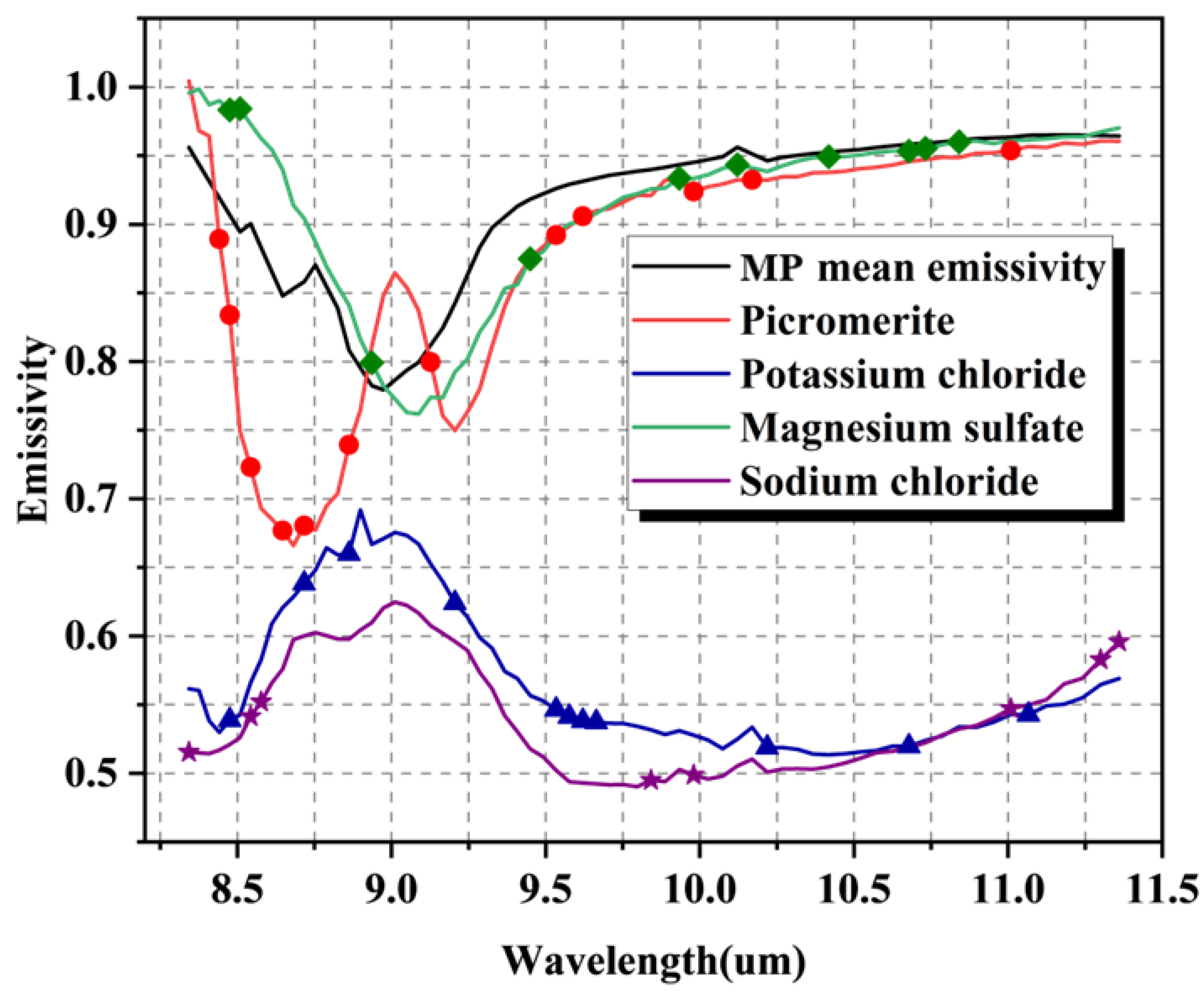
- TIH imaging revealed highly prominent emissivity characteristics of the MP samples in the thermal infrared band. Furthermore, the temperature discrepancy between the inverted and actual temperatures of the samples was relatively small, with 71% of the samples exhibiting a temperature difference of less than 1 K. This suggests that the emissivity accuracy of the samples obtained in this experimental process is high and can be approximated as the emissivity spectrum corresponding to potassium salt samples.
- (2)
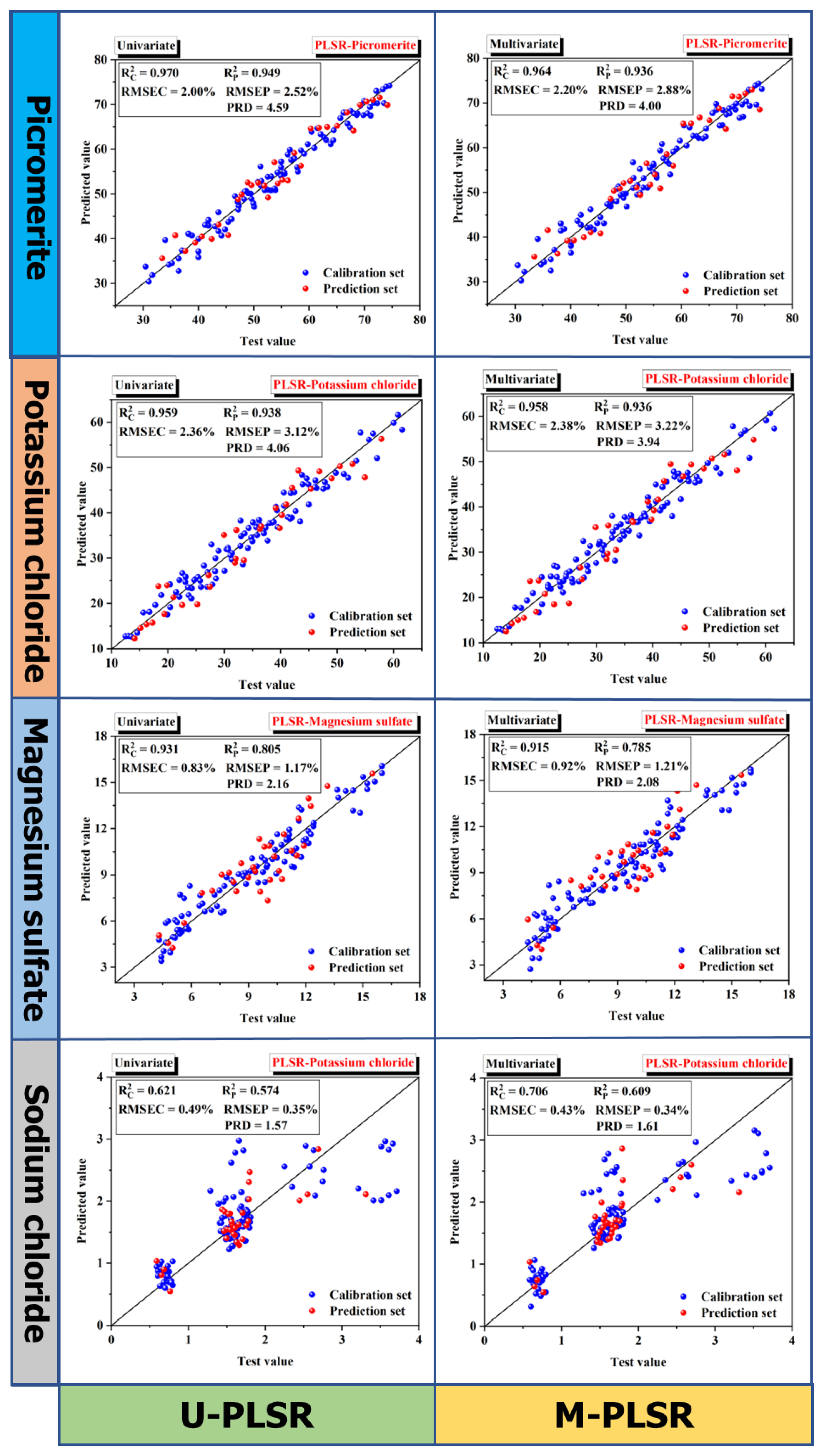
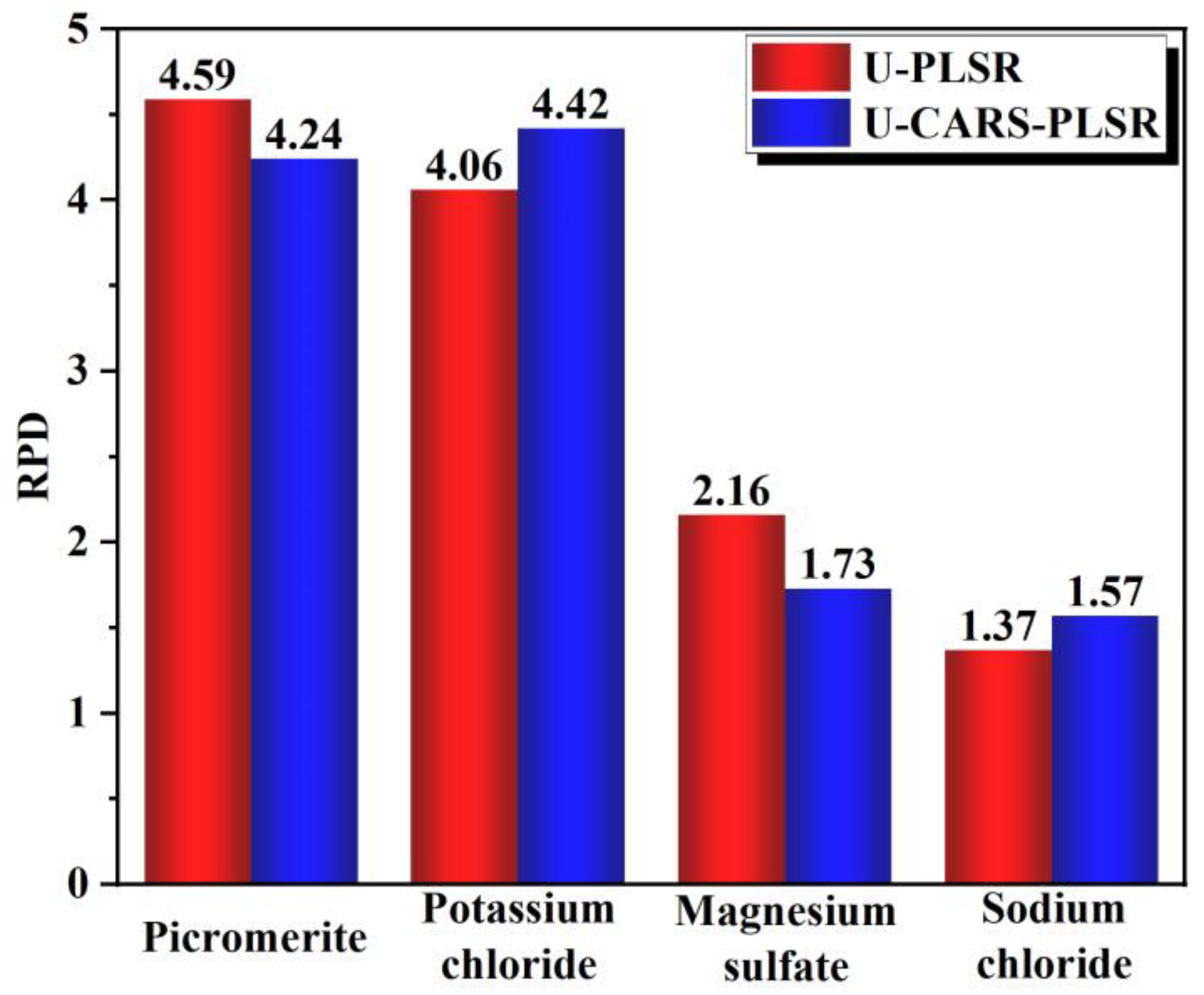
- The CARS-PLSR model, which is based on MP sample emissivity data training, is effective for MP sample prediction. In the U-PLSR model, the RPD values of the four minerals are 4.59, 4.06, 2.16, and 1.57, respectively, indicating that PLSR has a good prediction effect on MP. The calculation results of the U-CARS-PLSR model using the CARS method for sensitive wavelength selection show that the CARS method can effectively reduce the number of wavelengths, which is of great benefit to the practical application of TIH technology. With the CARS method, the number of selected wavelengths for the four minerals is reduced to 12, 11, 11, and 8, with RPD values of 4.24, 4.42, 1.73, and 1.37. The prediction accuracy of major minerals in MP is high (RPD > 4). The model has a good prediction effect on MP.
Author Contributions
Funding
Institutional Review Board Statement
Informed Consent Statement
Data Availability Statement
Acknowledgments
Conflicts of Interest
References
- Robben, C.; Wotruba, H. Sensor-Based Ore Sorting Technology in Mining—Past, Present and Future. Minerals 2019, 9, 523. [Google Scholar] [CrossRef] [Green Version]
- Kumar, V.; Kumar, A.; Lee, D.J.; Park, S.S. Estimation of Number of Graphene Layers Using Different Methods: A Focused Review. Materials 2021, 14, 4590. [Google Scholar] [CrossRef] [PubMed]
- Ahmad, A.; Abbasi, S.A.; Hafeez, M.; Khan, T.M.; Rafique, M.; Ahmed, N.; Ahmad, P.; Faruque, M.R.I.; Khandaker, M.U.; Javed, M. Detection and Quantification of Precious Elements in Astrophyllite Mineral by Optical Spectroscopy. Materials 2021, 14, 6277. [Google Scholar] [CrossRef] [PubMed]
- Resano, M.; Aramendía, M.; Nakadi, F.V.; García-Ruiz, E.; Alvarez-Llamas, C.; Bordel, N.; Pisonero, J.; Bolea-Fernández, E.; Liu, T.; Vanhaecke, F. Breaking the Boundaries in Spectrometry. Molecular Analysis with Atomic Spectrometric Techniques. TrAC-Trends Anal. Chem. 2020, 129, 115955. [Google Scholar] [CrossRef]
- Ge, L.; Li, F. Review of in situ X-ray fluorescence analysis technology in China. X-ray Spectrom. 2020, 49, 458–470. [Google Scholar] [CrossRef]
- Nair, A.G.C.; Sudarshan, K.; Raje, N.; Reddy, A.V.R.; Manohar, S.B.; Goswami, A. Analysis of Alloys by Prompt Gamma-Ray Neutron Activation. Nucl. Instrum. Methods Phys. Res. A 2004, 516, 143–148. [Google Scholar] [CrossRef]
- Ozaki, Y. Infrared Spectroscopy—Mid-Infrared, Near-Infrared, and Far-Infrared/Terahertz Spectroscopy. Anal. Sci. 2021, 37, 1193–1212. [Google Scholar] [CrossRef]
- Gupta, S.; Al-Obaidi, S.; Ferrara, L. Meta-Analysis and Machine Learning Models to Optimize the Efficiency of Self-Healing Capacity of Cementitious Material. Materials 2021, 14, 4437. [Google Scholar] [CrossRef]
- Hnilicová, M.; Turis, J.; Hnilica, R. Application of Multidimensional Statistical Analysis in Tribotechnical Diagnostics of Hydraulic Fluids in Woodworking EquiMPent. Materials 2021, 14, 4628. [Google Scholar] [CrossRef]
- Pasquini, C. Near Infrared Spectroscopy: A Mature Analytical Technique with New Perspectives—A Review. Anal. Chim. Acta 2018, 1026, 8–36. [Google Scholar] [CrossRef]
- Kaim, W. Concepts for Metal Complex Chromophores Absorbing in the near Infrared. Coord. Chem. Rev. 2011, 255, 2503–2513. [Google Scholar] [CrossRef]
- Velasco, F.; Alvaro, A.; Suarez, S.; Herrero, J.M.; Yusta, I. Mapping Fe-Bearing Hydrated Sulphate Minerals with Short Wave Infrared (SWIR) Spectral Analysis at San Miguel Mine Environment, Iberian Pyrite Belt (SW Spain). J. Geochem. Explor. 2005, 87, 45–72. [Google Scholar] [CrossRef]
- Simpson, M.P.; Rae, A.J. Short-Wave Infrared (SWIR) Reflectance Spectrometric Characterisation of Clays from Geothermal Systems of the Taupō Volcanic Zone, New Zealand. Geothermics 2018, 73, 74–90. [Google Scholar] [CrossRef]
- van der Meer, F.D.; van der Werff, H.M.A.; van Ruitenbeek, F.J.A.; Hecker, C.A.; Bakker, W.H.; Noomen, M.F.; van der Meijde, M.; Carranza, E.J.M.; de Smeth, J.B.; Woldai, T. Multi- and Hyperspectral Geologic Remote Sensing: A Review. Int. J. Appl. Earth Obs. Geoinf. 2012, 14, 112–128. [Google Scholar] [CrossRef]
- Christensen, P.R.; Bandfield, J.L.; Hamilton, V.E.; Howard, D.A.; Lane, M.D.; Piatek, J.L.; Ruff, S.W.; Stefanov, W.L. A Thermal Emission Spectral Library of Rock-Forming Minerals. J. Geophys. Res. Planets 2000, 105, 9735–9739. [Google Scholar] [CrossRef] [Green Version]
- Cui, J.; Yan, B.; Dong, X.; Zhang, S.; Zhang, J.; Tian, F.; Wang, R. Temperature and Emissivity Separation and Mineral Mapping Based on Airborne TASI Hyperspectral Thermal Infrared Data. Int. J. Appl. Earth Obs. Geoinf. 2015, 40, 19–28. [Google Scholar] [CrossRef]
- Christensen, P.R.; Jakosky, B.M.; Kieffer, H.H.; Malin, M.C.; Mcsween, H.Y.; Nealson, K.; Mehall, G.L.; Silverman, S.H.; Ferry, S.; Caplinger, M.; et al. The Thermal Emission Imaging System (Themis) for the Mars 2001 Odyssey Mission. Space Sci. Rev. 2004, 110, 85–130. [Google Scholar] [CrossRef]
- Pelkey, S.M.; Mustard, J.F.; Murchie, S.; Clancy, R.T.; Wolff, M.; Smith, M.; Milliken, R.E.; Bibring, J.P.; Gendrin, A.; Poulet, F.; et al. CRISM Multispectral Summary Products: Parameterizing Mineral Diversity on Mars from Reflectance. J. Geophys. Res. Planets 2007, 112, E8. [Google Scholar] [CrossRef]
- Mauger, A.J.; Ehrig, K.; Kontonikas-Charos, A.; Ciobanu, C.L.; Cook, N.J.; Kamenetsky, V.S. Alteration at the Olympic Dam IOCG–U Deposit: Insights into Distal to Proximal Feldspar and Phyllosilicate Chemistry from Infrared Reflectance Spectroscopy. Aust. J. Earth Sci. 2016, 63, 959–972. [Google Scholar] [CrossRef]
- Hamilton, V.E. Thermal Infrared (Vibrational) Spectroscopy of Mg-Fe Olivines: A Review and Applications to Determining the Composition of Planetary Surfaces. Chem. Erde 2010, 70, 7–33. [Google Scholar] [CrossRef]
- Yousefi, B.; Sojasi, S.; Castanedo, C.I.; Maldague, X.P.V.; Beaudoin, G.; Chamberland, M. Comparison Assessment of Low Rank Sparse-PCA Based-Clustering/Classification for Automatic Mineral Identification in Long Wave Infrared Hyperspectral Imagery. Infrared Phys. Technol. 2018, 93, 103–111. [Google Scholar] [CrossRef]
- Desta, F.; Buxton, M.; Jansen, J. Data Fusion for the Prediction of Elemental Concentrations in Polymetallic Sulphide Ore Using Mid-Wave Infrared and Long-Wave Infrared Reflectance Data. Minerals 2020, 10, 235. [Google Scholar] [CrossRef] [Green Version]
- Desta, F.; Buxton, M.; Jansen, J. Fusion of Mid-Wave Infrared and Long-Wave Infrared Reflectance Spectra for Quantitative Analysis of Minerals. Sensors 2020, 20, 1472. [Google Scholar] [CrossRef] [PubMed] [Green Version]
- Notesco, G.; Weksler, S.; Ben-Dor, E. Mineral Classification of Soils Using Hyperspectral Longwave Infrared (LWIR) Ground-Based Data. Remote Sens. 2019, 11, 1429. [Google Scholar] [CrossRef] [Green Version]
- Kopăcková, V.; Koucká, L. Integration of Absorption Feature Information from Visible to Longwave Infrared Spectral Ranges for Mineral Mapping. Remote Sens. 2017, 9, 1006. [Google Scholar] [CrossRef] [Green Version]
- Guzmán, Q.J.A.; Rivard, B.; Sánchez-Azofeifa, G.A. Discrimination of Liana and Tree Leaves from a Neotropical Dry Forest Using Visible-near Infrared and Longwave Infrared Reflectance Spectra. Remote Sens. Environ. 2018, 219, 135–144. [Google Scholar] [CrossRef]
- Weksler, S.; Rozenstein, O.; Ben-Dor, E. Mapping Surface Quartz Content in Sand Dunes Covered by Biological Soil Crusts Using Airborne Hyperspectral Images in the Longwave Infrared Region. Minerals 2018, 8, 318. [Google Scholar] [CrossRef] [Green Version]
- Laakso, K.; Turner, D.J.; Rivard, B.; Sánchez-Azofeifa, A. The Long-Wave Infrared (8–12 μm) Spectral Features of Selected Rare Earth Element—Bearing Carbonate, Phosphate and Silicate Minerals. Int. J. Appl. Earth Obs. Geoinf. 2019, 76, 77–83. [Google Scholar] [CrossRef]
- Manolakis, D.; Pieper, M.; Truslow, E.; Lockwood, R.; Weisner, A.; Jacobson, J.; Cooley, T. Longwave Infrared Hyperspectral Imaging: Principles, Progress, and Challenges. IEEE Geosci. Remote Sens. Mag. 2019, 7, 72–100. [Google Scholar] [CrossRef]
- Bunaciu, A.A.; Udriştioiu, E.g.; Aboul-Enein, H.Y. X-ray Diffraction: Instrumentation and Applications. Crit. Rev. Anal. Chem. 2015, 45, 289–299. [Google Scholar] [CrossRef]
- Labranche, N.; Teale, K.; Wightman, E.; Johnstone, K.; Cliff, D. Characterization Analysis of Airborne Particulates from Australian Underground Coal Mines Using the Mineral Liberation Analyser. Minerals 2022, 12, 796. [Google Scholar] [CrossRef]
- Es’kina, V.V.; Dal’nova, O.A.; Tursunov, L.K.; Baranovskaya, V.B.; Karpov, Y.A. Detection of Sodium in Highly Pure Graphite via High-Resolution Electrothermal Atomic Absorption Spectrometry with a Continuous Spectrum Source. Inorg. Mater. 2018, 53, 1379–1381. [Google Scholar] [CrossRef]
- Gao, L.; Cao, L.; Zhong, Y.; Jia, Z. Field-Based High-Quality Emissivity Spectra Measurement Using a Fourier Transform Thermal Infrared Hyperspectral Imager. Remote Sens. 2021, 13, 4453. [Google Scholar] [CrossRef]
- Ingram, M.P.; Muse, A.H. Sensitivity of iterative spectrally smooth temperature/emissivity separation to algorithmic assumptions and measurement noise. IEEE Trans. Geosci. Remote Sens. 2001, 39, 2158–2167. [Google Scholar] [CrossRef]
- Li, Z.L.; Wu, H.; Wang, N.; Qiu, S.; Sobrino, J.A.; Wan, Z.; Tang, B.H.; Yan, G. Land Surface Emissivity Retrieval from Satellite Data. Int. J. Remote Sens. 2013, 34, 3084–3127. [Google Scholar] [CrossRef]
- Zimek, A.; Filzmoser, P. There and Back Again: Outlier Detection between Statistical Reasoning and Data Mining Algorithms. Wiley Interdiscip. Rev. Data Min. Knowl. Discov. 2018, 8, e1280. [Google Scholar] [CrossRef] [Green Version]
- Verrelst, J.; Camps-Valls, G.; Muñoz-Marí, J.; Rivera, J.P.; Veroustraete, F.; Clevers, J.G.P.W.; Moreno, J. Optical Remote Sensing and the Retrieval of Terrestrial Vegetation Bio-Geophysical Properties—A Review. ISPRS J. Photogramm. Remote Sens. 2015, 108, 273–290. [Google Scholar] [CrossRef]
- Li, H.; Liang, Y.; Xu, Q.; Cao, D. Key Wavelengths Screening Using Competitive Adaptive Reweighted Sampling Method for Multivariate Calibration. Anal. Chim. Acta 2009, 648, 77–84. [Google Scholar] [CrossRef]
- Zhang, C.; Liu, F.; Kong, W.; He, Y. Application of Visible and Near-Infrared Hyperspectral Imaging to Determine Soluble Protein Content in Oilseed Rape Leaves. Sensors 2015, 15, 16576–16588. [Google Scholar] [CrossRef] [Green Version]


| Mineral Name | Weight (%) | Area (%) | Area (μm2) | Particle Number | Statistical Relative Error(%) |
|---|---|---|---|---|---|
| Picromerite | 64.60 | 55.29 | 10,332,530.00 | 74,425.00 | 0.01 |
| Potassium chloride | 29.05 | 35.36 | 6,607,637.00 | 44,909.00 | 0.01 |
| Low count rate | 5.37 | 8.18 | 1,528,364.25 | 185,661.00 | 0.00 |
| Unknown minerals | 0.96 | 1.17 | 218,234.56 | 2525.00 | 0.04 |
| Sodium chloride | 0.01 | 0.01 | 1517.26 | 18.00 | 0.47 |
| Ion Species | K+ | Mg2+ | Cl− | Na+ | |
|---|---|---|---|---|---|
| Content(%) | 27.18 | 4.30 | 33.67 | 13.57 | 0.32 |
| Sum | Mean (%) | Standard Deviation (%) | Minimum (%) | Median (%) | Maximum (%) | ||
|---|---|---|---|---|---|---|---|
| Group one | Picromerite | 738 | 51.20 | 6.14 | 30.73 | 51.19 | 76.79 |
| Potassium chloride | 35.94 | 4.98 | 17.39 | 36.13 | 52.50 | ||
| Magnesium sulfate | 10.31 | 2.43 | 2.25 | 10.11 | 17.93 | ||
| Sodium chloride | 2.55 | 0.71 | 0.97 | 2.56 | 5.51 | ||
| Group two | Picromerite | 138 | 53.91 | 11.67 | 30.46 | 53.43 | 74.49 |
| Potassium chloride | 34.59 | 12.05 | 12.46 | 33.88 | 61.52 | ||
| Magnesium sulfate | 9.26 | 3.10 | 4.30 | 9.53 | 16.00 | ||
| Sodium chloride | 1.65 | 0.75 | 0.59 | 1.59 | 3.73 | ||
| Sum | Mean (%) | Standard Deviation (%) | Minimum (%) | Median (%) | Maximum (%) | ||
|---|---|---|---|---|---|---|---|
| Calibration set | Picromerite | 97 | 54.05 | 11.67 | 30.46 | 53.76 | 74.49 |
| Potassium chloride | 34.50 | 11.73 | 12.46 | 34.17 | 61.52 | ||
| Magnesium sulfate | 9.24 | 3.23 | 4.30 | 9.43 | 16.00 | ||
| Sodium chloride | 1.65 | 0.80 | 0.59 | 1.59 | 3.71 | ||
| Prediction set | Picromerite | 32 | 54.54 | 11.55 | 33.45 | 54.03 | 74.10 |
| Potassium chloride | 33.68 | 12.66 | 14.05 | 32.80 | 57.84 | ||
| Magnesium sulfate | 9.46 | 2.52 | 4.30 | 9.72 | 15.51 | ||
| Sodium chloride | 1.64 | 0.55 | 0.59 | 1.61 | 3.31 | ||
| Calibration Set | Prediction Set | |||||
|---|---|---|---|---|---|---|
| RMSEC | RMSEP | RPD | ||||
| U-PLSR | Picromerite | 0.970 | 2.00% | 0.949 | 2.52% | 4.59 |
| Potassium chloride | 0.959 | 2.36% | 0.938 | 3.12% | 4.06 | |
| Magnesium sulfate | 0.931 | 0.83% | 0.805 | 1.17% | 2.16 | |
| Sodium chloride | 0.621 | 0.49% | 0.574 | 0.35% | 1.57 | |
| M-PLSR | Picromerite | 0.964 | 2.20% | 0.936 | 2.88% | 4.00 |
| Potassium chloride | 0.958 | 2.38% | 0.936 | 3.22% | 3.94 | |
| Magnesium sulfate | 0.915 | 0.92% | 0.785 | 1.21% | 2.08 | |
| Sodium chloride | 0.706 | 0.43% | 0.609 | 0.34% | 1.61 | |
| Mineral Species | Number | Sensitive Wavelengths (μm) |
|---|---|---|
| Picromerite | 12 | 8.44, 8.48, 8.54, 8.65, 8.72, 8.86, 9.13, 9.53, 9.62, 9.98, 10.17, 11.01 |
| Potassium chloride | 11 | 8.48, 8.72, 8.86, 9.21, 9.53, 9.58, 9.62, 9.66, 10.22, 10.68, 11.07 |
| Magnesium sulfate | 11 | 8.48, 8.51, 8.94, 9.45, 9.62, 9.93, 10.12, 10.42, 10.68, 10.73, 10.84 |
| Sodium chloride | 8 | 8.34, 8.54, 8.58, 9.84, 9.98, 11.01, 11.30, 11.36 |
| Calibration Set | Prediction Set | |||||
|---|---|---|---|---|---|---|
| RMSEC | RMSEP | RPD | ||||
| U-CARS-PLSR | Picromerite | 0.968 | 2.05% | 0.943 | 2.72% | 4.24 |
| Potassium chloride | 0.959 | 2.36% | 0.948 | 2.86% | 4.42 | |
| Magnesium sulfate | 0.868 | 1.15% | 0.690 | 1.45% | 1.73 | |
| Sodium chloride | 0.682 | 0.44% | 0.485 | 0.40% | 1.37 | |
| M-CARS-PLSR | Picromerite | 0.964 | 2.20% | 0.940 | 2.78% | 4.15 |
| Potassium chloride | 0.955 | 2.47% | 0.938 | 3.16% | 4.00 | |
| Magnesium sulfate | 0.922 | 0.88% | 0.770 | 1.29% | 1.96 | |
| Sodium chloride | 0.715 | 0.42% | 0.500 | 0.40% | 1.36 | |
Disclaimer/Publisher’s Note: The statements, opinions and data contained in all publications are solely those of the individual author(s) and contributor(s) and not of MDPI and/or the editor(s). MDPI and/or the editor(s) disclaim responsibility for any injury to people or property resulting from any ideas, methods, instructions or products referred to in the content. |
© 2023 by the authors. Licensee MDPI, Basel, Switzerland. This article is an open access article distributed under the terms and conditions of the Creative Commons Attribution (CC BY) license (https://creativecommons.org/licenses/by/4.0/).
Share and Cite
Qi, M.; Cao, L.; Zhao, Y.; Jia, F.; Song, S.; He, X.; Yan, X.; Huang, L.; Yin, Z. Quantitative Analysis of Mixed Minerals with Finite Phase Using Thermal Infrared Hyperspectral Technology. Materials 2023, 16, 2743. https://doi.org/10.3390/ma16072743
Qi M, Cao L, Zhao Y, Jia F, Song S, He X, Yan X, Huang L, Yin Z. Quantitative Analysis of Mixed Minerals with Finite Phase Using Thermal Infrared Hyperspectral Technology. Materials. 2023; 16(7):2743. https://doi.org/10.3390/ma16072743
Chicago/Turabian StyleQi, Meixiang, Liqin Cao, Yunliang Zhao, Feifei Jia, Shaoxian Song, Xinfang He, Xiao Yan, Lixue Huang, and Zize Yin. 2023. "Quantitative Analysis of Mixed Minerals with Finite Phase Using Thermal Infrared Hyperspectral Technology" Materials 16, no. 7: 2743. https://doi.org/10.3390/ma16072743