
Uncertainty Quantification in Constitutive Models of Highway Bridge Components: Seismic Bars and Elastomeric Bearings
 ,
,
Abstract
:1. Introduction
2. Experimental Data
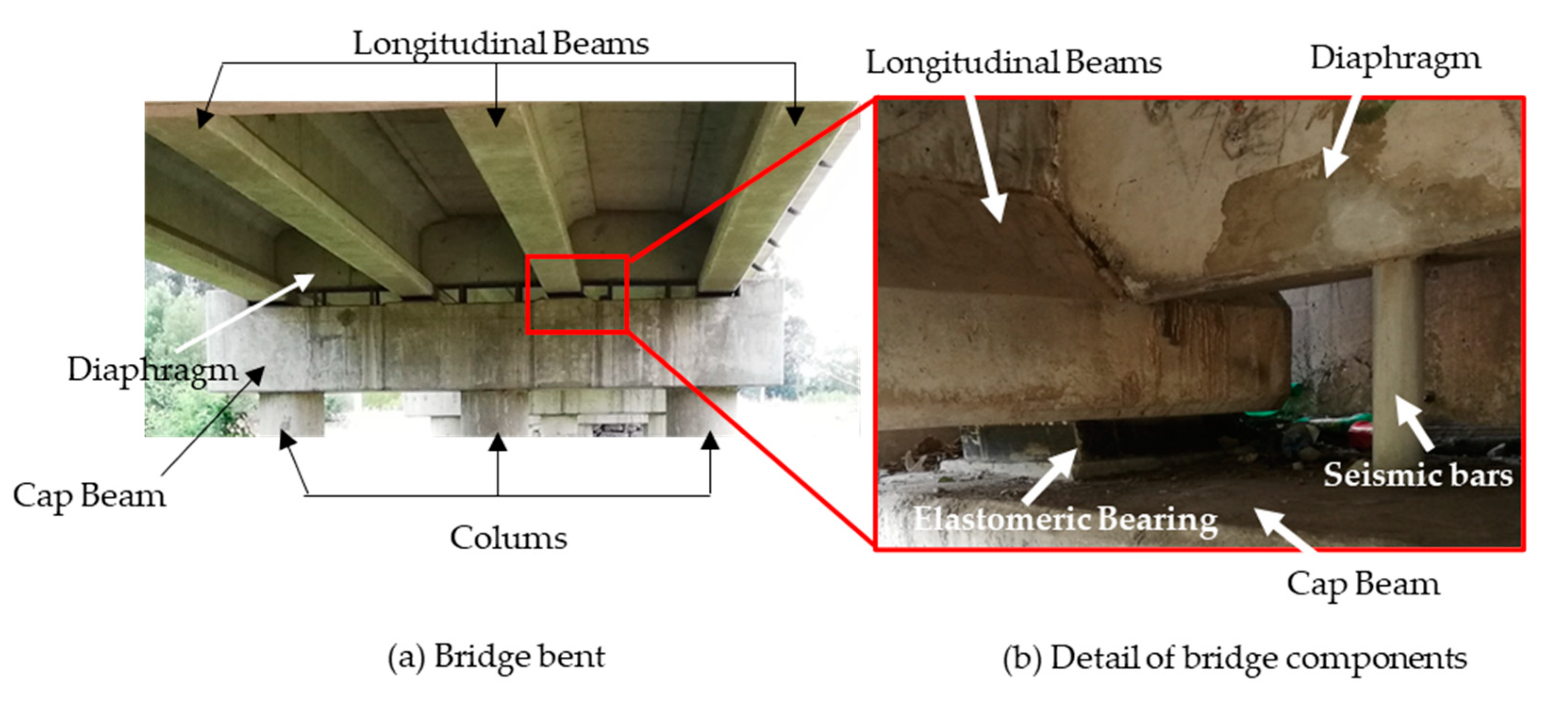
2.1. Seismic Bars (SBs)
2.2. Elastomeric Bearings (EBs)
2.2.1. Unanchored Elastomeric Bearing (UEB)
2.2.2. Anchored Elastomeric Bearing (AEB)
3. Constitutive Models
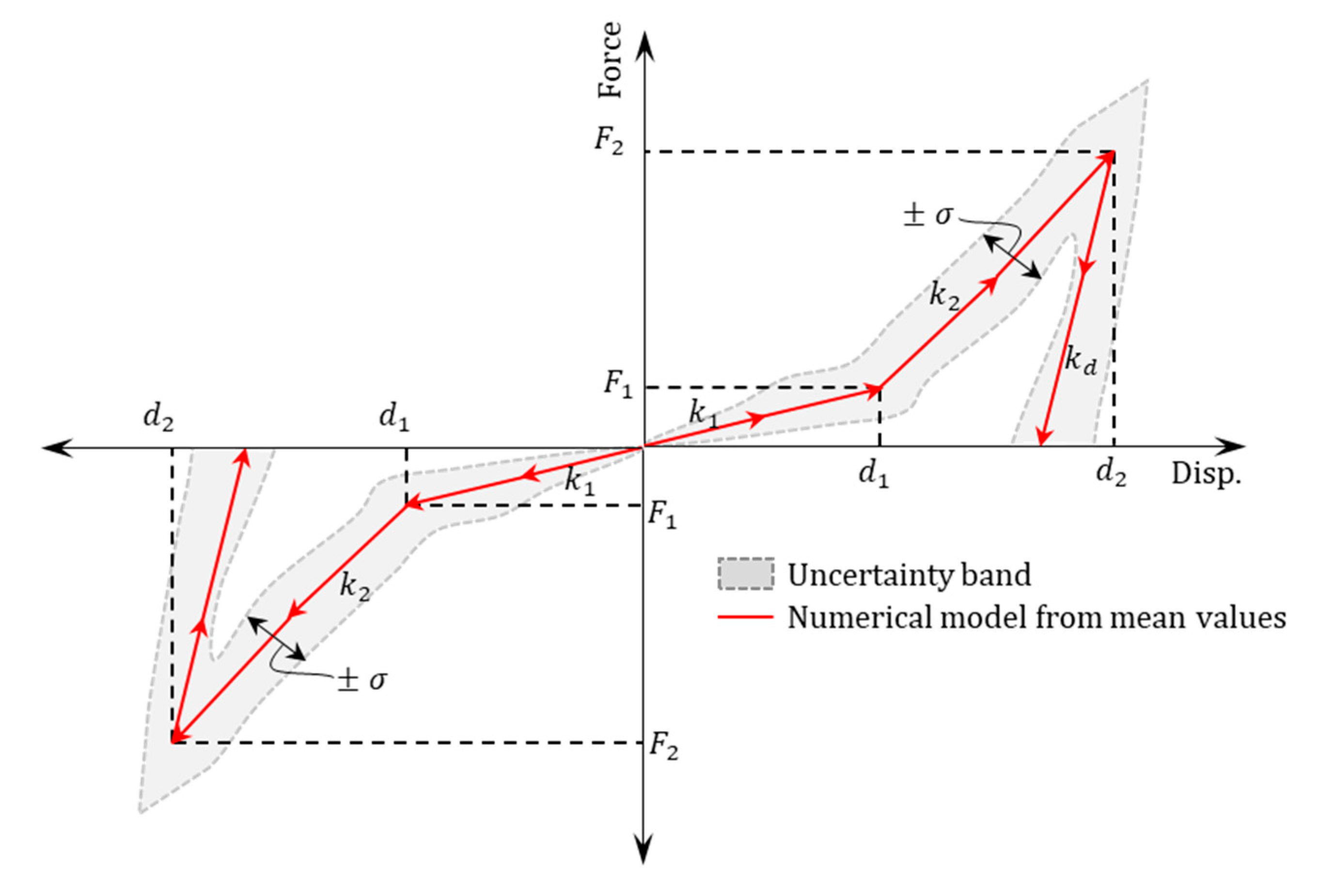
3.1. Seismic Bars (SBs)
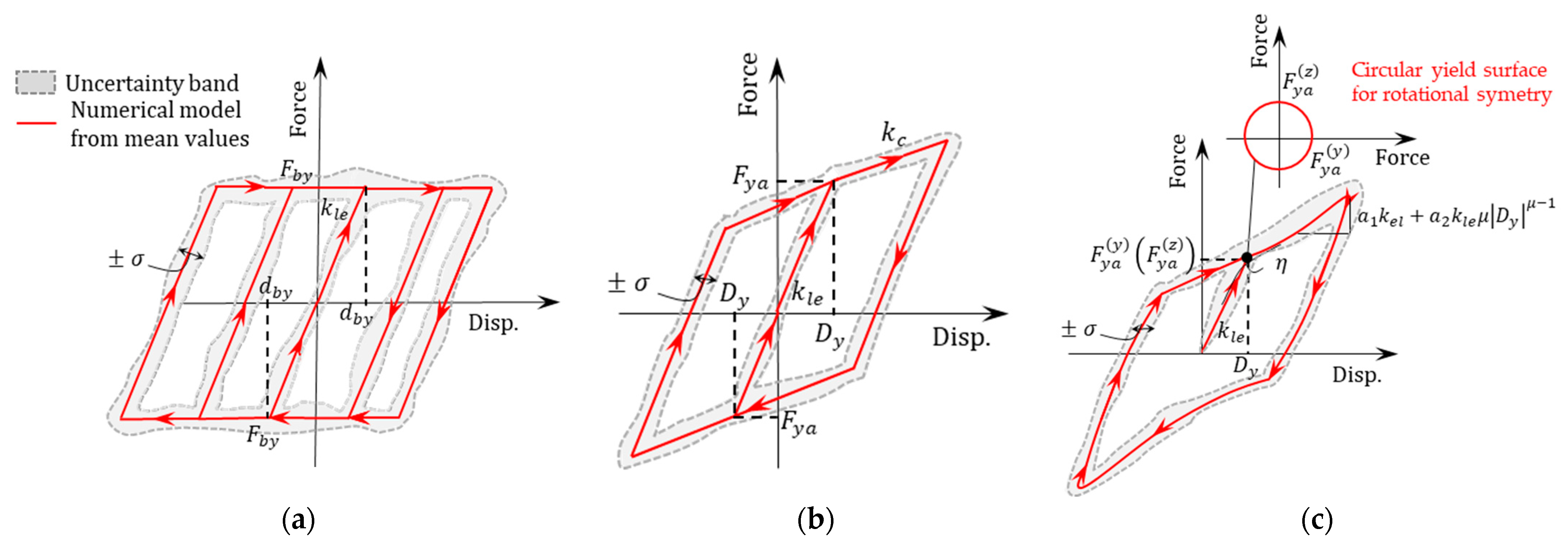
3.2. Elastomeric Bearings
3.2.1. Unanchored Elastomeric Bearing (UEB)
3.2.2. Anchored Elastomeric Bearing (AEB)
4. Bayesian Parameter Estimation
4.1. Bayesian Inversion
4.2. Markov Chain Monte Carlo (MCMC)
4.3. Tempering
- Sample each parameter from a prior distribution.
- Simulate a dataset using a function that takes the parameters and returns the predicted data (), considering the dimension of the observed data.
- Compare and using the distance function and a tolerance threshold value.
- When , the distance function value is less than the threshold value; if this tolerance value is sufficiently small, the distribution obtained will be a good approximation for the posterior
4.4. Convergence Criteria
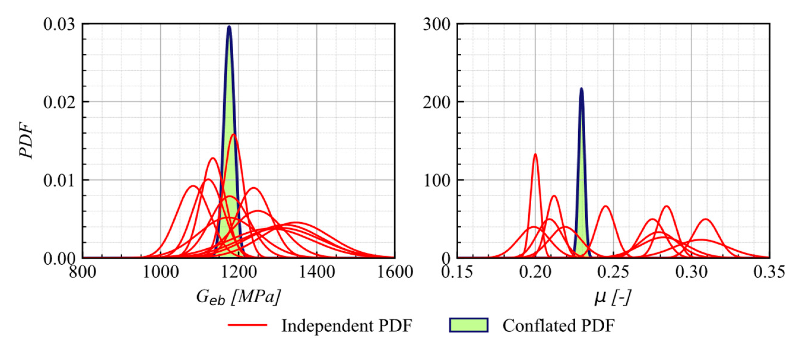
4.5. Conflation Procedure
5. Results and Discussion
5.1. Calibration
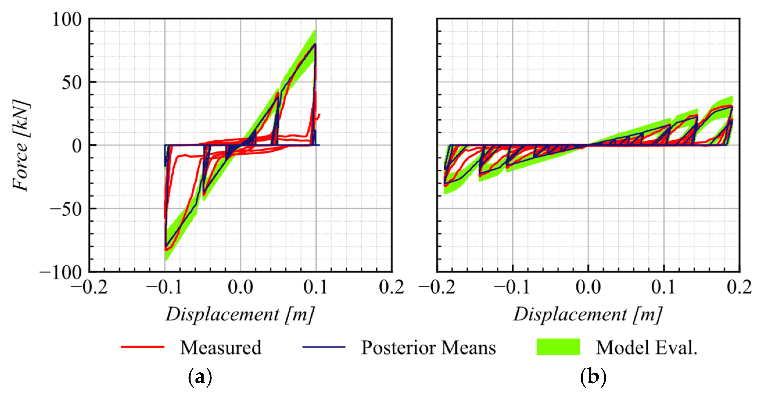
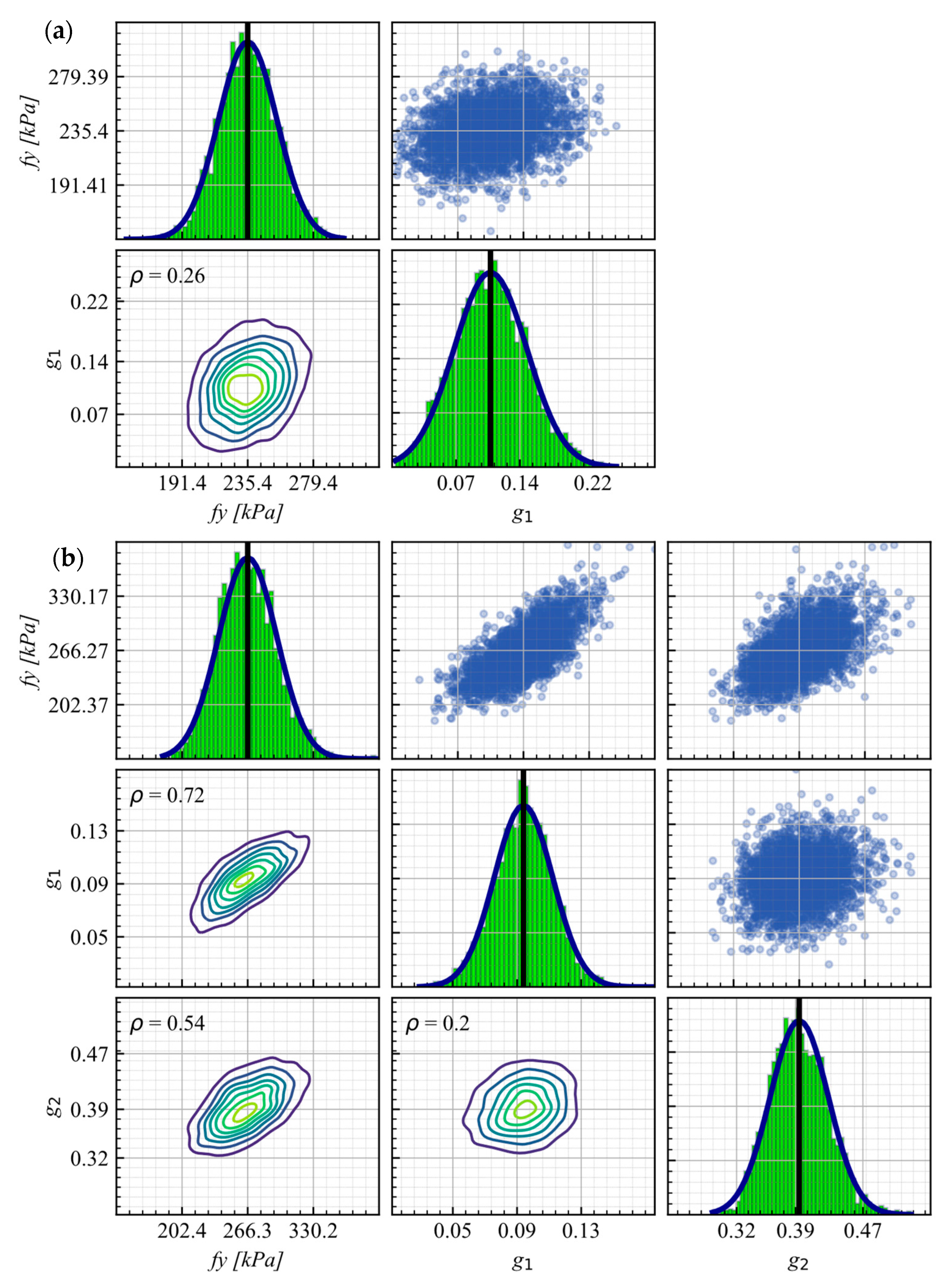
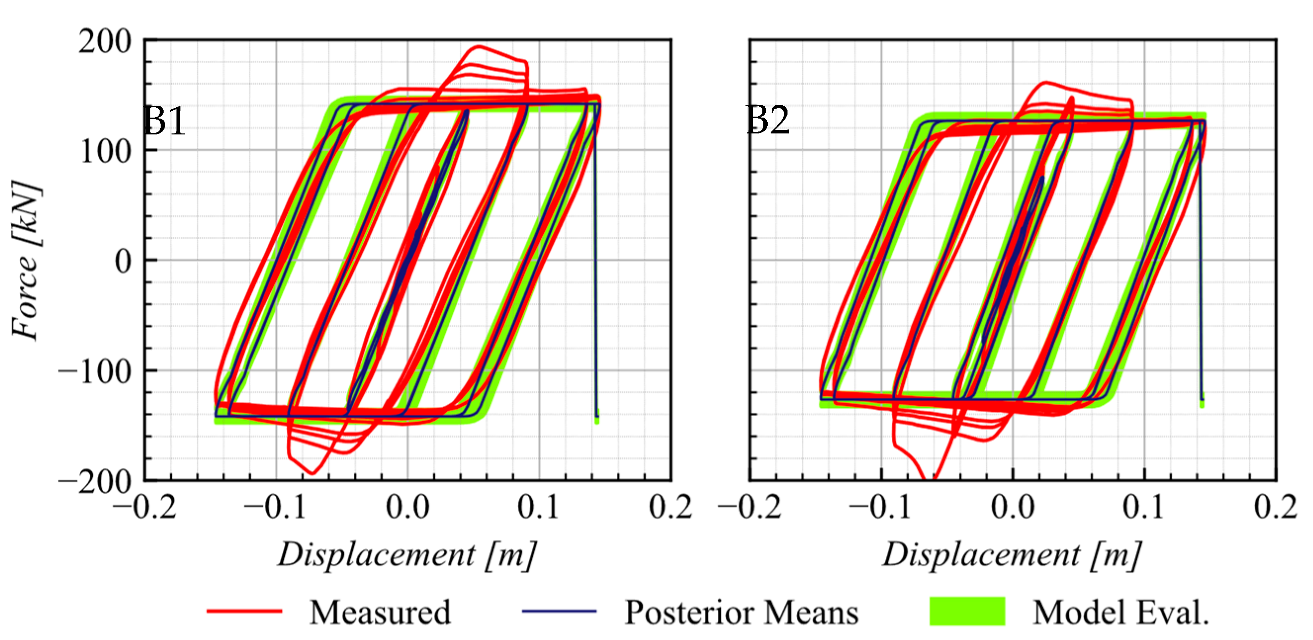
5.1.1. Seismic Bars (SBs)
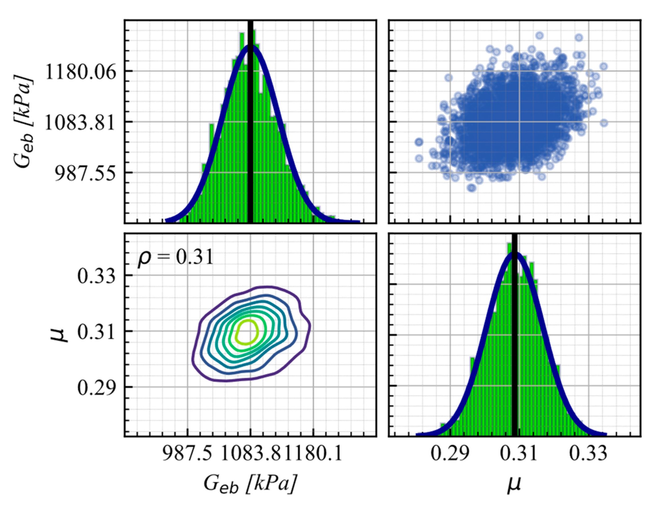
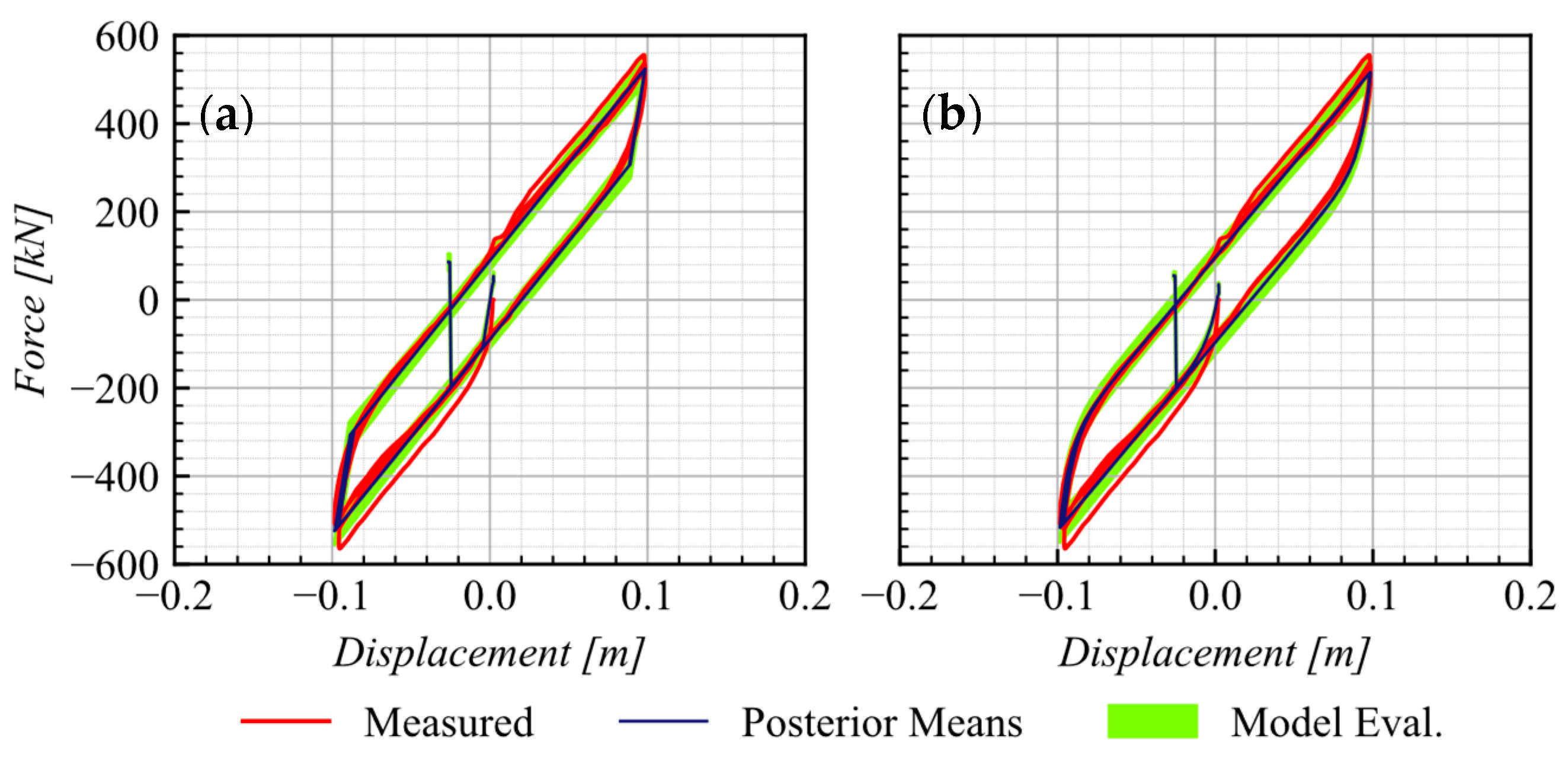
5.1.2. UEB
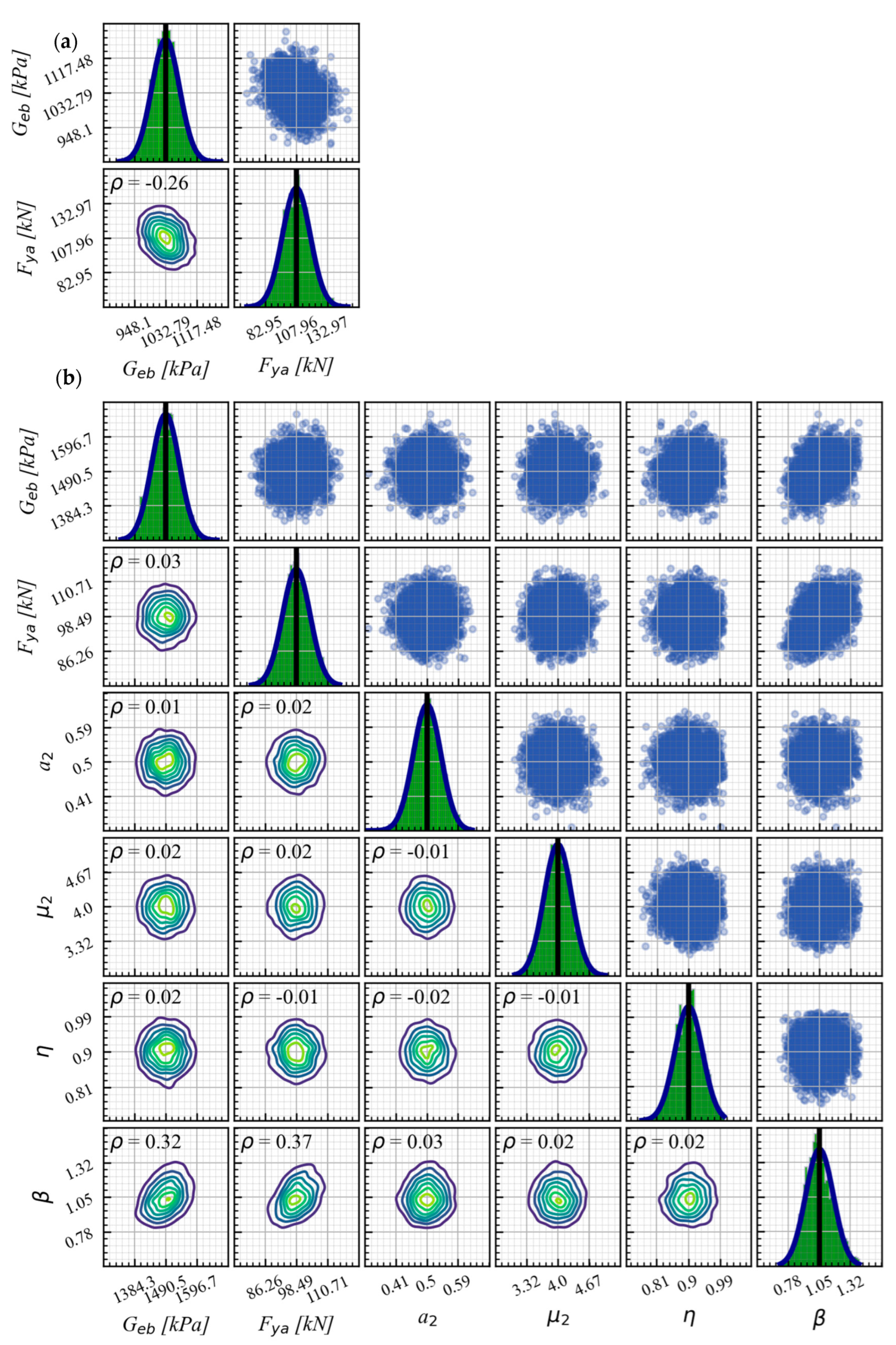
5.1.3. AEB
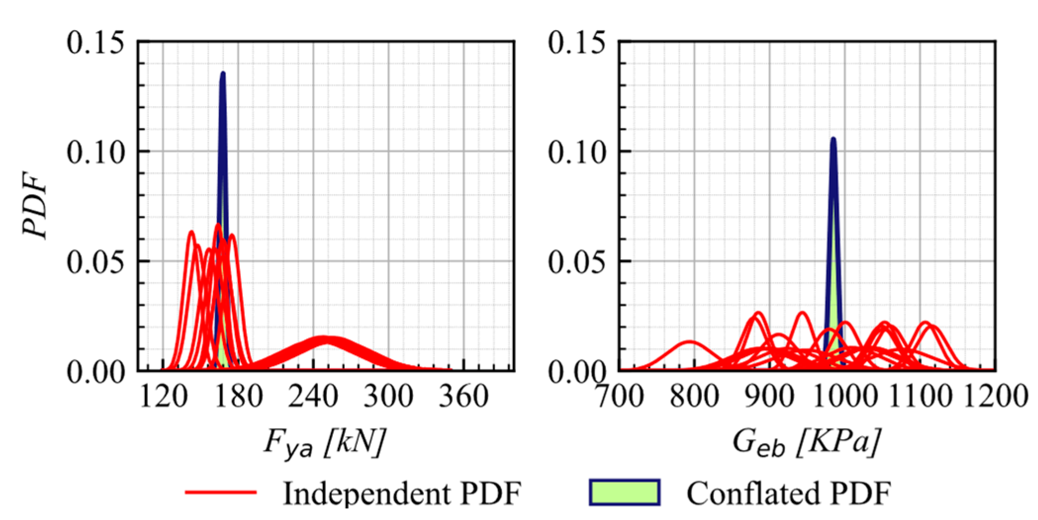
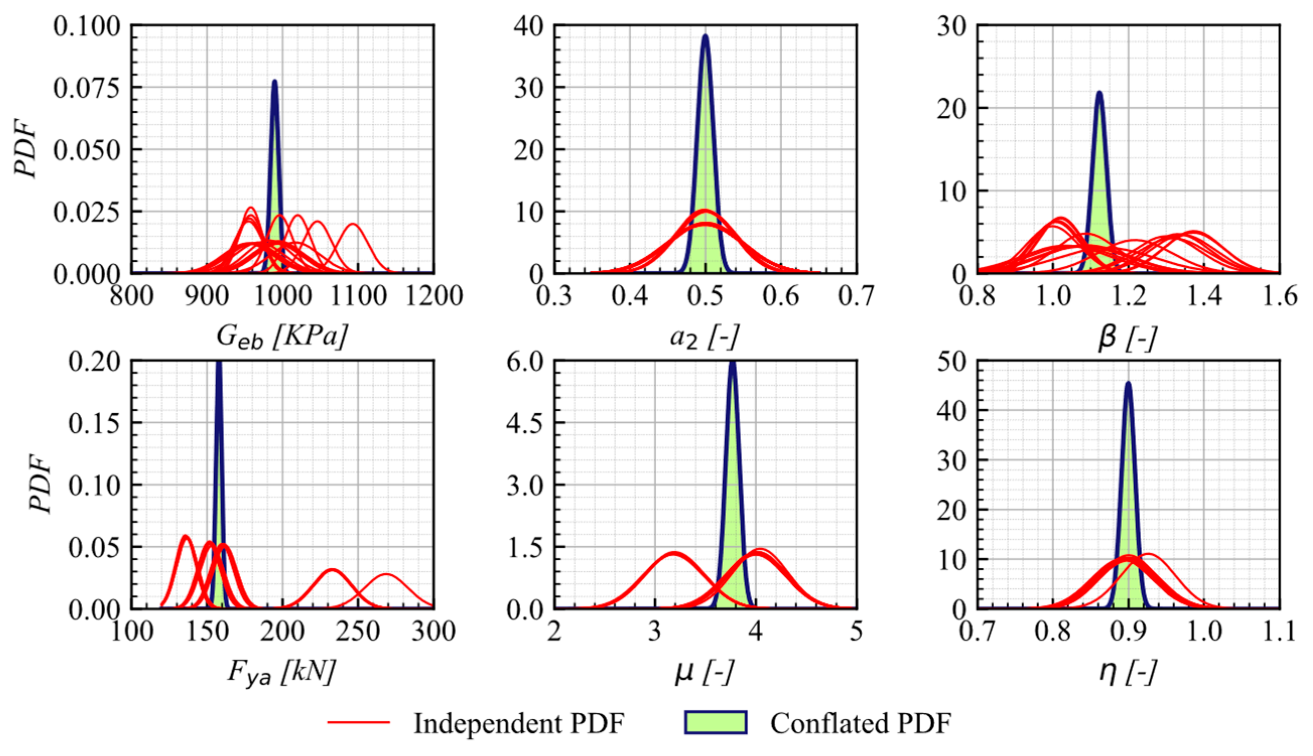
5.2. Proposed PDFs
6. Conclusions
Author Contributions
Funding
Informed Consent Statement
Data Availability Statement
Acknowledgments
Conflicts of Interest
References
- SEAOC. A Framework of Performance-Based Seismic Engineering of Buildings; Structural Engineers Association of California: Sacramento, CA, USA, 1995. [Google Scholar]
- ASCE. Seismic Design of Piers and Wharves; ASCE: Reston, VA, USA, 2014; p. 61. [Google Scholar] [CrossRef]
- Tall Building Initiative (TBI). Guidelines for Performance-Based Seismic Design of Tall Buildings; TBI: Berkeley, CA, USA, 2017. [Google Scholar]
- Zhang, P.; Restrepo, J.I.; Conte, J.P.; Ou, J. Nonlinear Finite Element Modeling and Response Analysis of the Collapsed Alto Rio Building in the 2010 Chile Maule Earthquake. Struct. Tall Spec. Build. 2017, 26, e1364. [Google Scholar] [CrossRef]
- Hube, M.; Santa María, H.; Villalobos, F. Preliminary Analysis of the Seismic Response of Bridges during the Chilean 27 February 2010 Earthquake. Obras Proy. Rev. Ing. Civ. 2010, 8, 48–57. [Google Scholar]
- Elnashai, A.S.; Gencturk, B.; Kwon, O.S.; Hashash, Y.M.A.; Kim, S.J.; Jeong, S.H.; Dukes, J. The Maule (Chile) Earthquake of February 27, 2010: Development of Hazard, Site Specific Ground Motions and Back-Analysis of Structures. Soil Dyn. Earthq. Eng. 2012, 42, 229–245. [Google Scholar] [CrossRef]
- Wilches, J.; Santa María, H.; Riddell, R.; Arrate, C. Effects of Changes in Seismic Design Criteria in the Transverse and Vertical Response of Chilean Highway Bridges. Eng. Struct. 2019, 191, 370–385. [Google Scholar] [CrossRef]
- Aldea, S.; Bazaez, R.; Astroza, R.; Hernandez, F. Seismic Fragility Assessment of Chilean Skewed Highway Bridges. Eng. Struct. 2021, 249, 113300. [Google Scholar] [CrossRef]
- Martínez, A.; Hube, M.A.; Rollins, K.M. Analytical Fragility Curves for Non-Skewed Highway Bridges in Chile. Eng. Struct. 2017, 141, 530–542. [Google Scholar] [CrossRef]
- Xiang, N.; Goto, Y.; Alam, M.S.; Li, J. Effect of Bonding or Unbonding on Seismic Behavior of Bridge Elastomeric Bearings: Lessons Learned from Past Earthquakes in China and Japan and Inspirations for Future Design. Adv. Bridge Eng. 2021, 2, 1–17. [Google Scholar] [CrossRef]
- Aviram, A.; Mackie, K.R.; Stojadinovic, B. Nonlinear Modeling of Bridge Structures in California. ACI Symp. Publ. 2010, 271, 1–26. [Google Scholar] [CrossRef]
- Steelman, J.S.; Fahnestock, L.A.; Filipov, E.T.; LaFave, J.M.; Hajjar, J.F.; Foutch, D.A. Shear and Friction Response of Nonseismic Laminated Elastomeric Bridge Bearings Subject to Seismic Demands. J. Bridge Eng. 2013, 18, 612–623. [Google Scholar] [CrossRef]
- Filipov, E.T.; Fahnestock, L.A.; Steelman, J.S.; Hajjar, J.F.; LaFave, J.M.; Foutch, D.A. Evaluation of Quasi-Isolated Seismic Bridge Behavior Using Nonlinear Bearing Models. Eng. Struct. 2013, 49, 168–181. [Google Scholar] [CrossRef]
- Konstantinidis, D.; Kelly, J.M.; Makris, N. Experimental Investigation on the Seismic Response of Bridge Bearings; Earthquake Engineering Research Center, University of California: Berkeley, CA, USA, 2008. [Google Scholar]
- Rubilar, F. Modelo no Lineal Para Predecir la Respuesta Sísmica de Pasos Superiores; Pontificia Universidad Católica de Chile: Santiago, Chile, 2015. [Google Scholar]
- Astroza, R.; Alessandri, A.; Conte, J.P. A Dual Adaptive Filtering Approach for Nonlinear Finite Element Model Updating Accounting for Modeling Uncertainty. Mech. Syst. Signal Process. 2019, 115, 782–800. [Google Scholar] [CrossRef]
- Ebrahimian, H.; Astroza, R.; Conte, J.P.; de Callafon, R.A. Nonlinear Finite Element Model Updating for Damage Identification of Civil Structures Using Batch Bayesian Estimation. Mech. Syst. Signal Process. 2017, 84, 194–222. [Google Scholar] [CrossRef]
- Birrell, M.; Astroza, R.; Carreño, R.; Restrepo, J.I.; Araya-Letelier, G. Bayesian Parameter and Joint Probability Distribution Estimation for a Hysteretic Constitutive Model of Reinforcing Steel. Struct. Saf. 2021, 90, 102062. [Google Scholar] [CrossRef]
- McKenna, F.; Fenves, G.L.; Scott, M.H. Open System for Earthquake Engineering Simulation; Pacific Earthquake Engineering Research Center, University of California: Berkeley, CA, USA, 2003. [Google Scholar]
- AASHTO. LRFD. Bridge Design Specifications, 8th ed.; American Association of State Highway and Transportation Officials: Washington, DC, USA, 2017. [Google Scholar]
- Wen, Y.-K. Method for Random Vibration of Hysteretic Systems. J. Eng. Mech. Div. 1976, 102, 249–263. [Google Scholar] [CrossRef]
- Yi, J.; Yang, H.; Li, J. Experimental and Numerical Study on Isolated Simply-Supported Bridges Subjected to a Fault Rupture. Soil Dyn. Earthq. Eng. 2019, 127, 105819. [Google Scholar] [CrossRef]
- Toni, T.; Welch, D.; Strelkowa, N.; Ipsen, A.; Stumpf, M.P.H. Approximate Bayesian Computation Scheme for Parameter Inference and Model Selection in Dynamical Systems. J. R. Soc. Interface 2009, 6, 187–202. [Google Scholar] [CrossRef] [Green Version]
- Ramancha, M.K.; Astroza, R.; Madarshahian, R.; Conte, J.P. Bayesian Updating and Identifiability Assessment of Nonlinear Finite Element Models. Mech. Syst. Signal Process. 2022, 167, 108517. [Google Scholar] [CrossRef]
- Chib, S.; Greenberg, E. Understanding the Metropolis-Hastings Algorithm. Am. Stat. 1995, 49, 327–335. [Google Scholar] [CrossRef] [Green Version]
- Kroese, D.P.; Taimre, T.; Botev, Z.I. Handbook of Monte Carlo Methods; John Wiley & Sons: Hoboken, NJ, USA, 2013. [Google Scholar]
- Wagner, P.R.; Nagel, J.; Marelli, S.; Sudret, B. UQLab User Manual—Bayesian Inference for Model Calibration and Inverse Problems; Report No. UQLab-V1. In Chair of Risk, Safety & Uncertainty Quantification; ETH Zurich: Zürich, Switzerland, 2019; pp. 3–113. [Google Scholar]
- Lintusaari, J.; Gutmann, M.U.; Kaski, S.; Corander, J. On the Identifiability of Transmission Dynamic Models for Infectious Diseases. Genetics 2016, 202, 911–918. [Google Scholar] [CrossRef] [Green Version]
- Vats, D.; Flegal, J.M.; Jones, G.L. Multivariate Output Analysis for Markov Chain Monte Carlo. Biometrika 2019, 106, 321–337. [Google Scholar] [CrossRef] [Green Version]
- Hill, T.P.; Miller, J. How to Combine Independent Data Sets for the Same Quantity. Chaos: Interdiscip. J. Nonlinear Sci. 2011, 21, 033102. [Google Scholar] [CrossRef] [PubMed] [Green Version]
- Neal, R.M. Slice Sampling. Ann. Stat. 2003, 31, 705–767. [Google Scholar] [CrossRef]
- Gelman, A.; Rubin, D.B. Inference from Iterative Simulation Using Multiple Sequences. Stat. Sci. 1992, 7, 457–472. [Google Scholar] [CrossRef]
- AASHTO. LRFD Bridge Design Specifications, 6th ed.; American Association of State Highway and Transportation Officials: Washington, DC, USA, 2012. [Google Scholar]


| Specimen | hl (cm) |
|---|---|
| WD1/WD2 | 10 |
| WOD1/WOD2 | 72 |
| Test Tag | Cyclic Test Velocity (mm/s) |
|---|---|
| B1 | 25 |
| B2 | 25 |
| B3 | 10 |
| B4 | 50 |
| B5 | 75 |
| B6 | 100 |
| Test Series | N | Width (mm) | Length (mm) | Diameter (mm) | Total Height (mm) |
|---|---|---|---|---|---|
| S1 | 5 | 650 | 650 | - | 98 |
| S2 | 4 | - | - | 500 | 100 |
| S3 | 6 | 320 | 320 | - | 53 |
| S4 | 4 | 700 | 700 | - | 194 |
| 4 | 1000 | 1000 | - | 230 | |
| S5 | 1 | 585 | 600 | - | 168 |
| Type of Seismic Bar | ||
|---|---|---|
| SBs-WD | 0.04 | 0.71 |
| SBs-WOD | 0.07 | 0.31 |
| Parameter | |
|---|---|
| Post-yield stiffness ratio of non-linear hardening component | |
| Exponent of non-linear hardening component | |
| Yield exponent | |
| First hysteretic shape parameter | |
| Parameter | Distribution | Mean | COV (%) | |
|---|---|---|---|---|
| SBs-WD (WD2) | (MPa) | Normal | 235.46 | 5.82 |
| (-) | 0.11 | 36.36 | ||
| SBs-WOD (WOD1) | (MPa) | Normal | 266.24 | 8.40 |
| (-) | 0.09 | 22.22 | ||
| (-) | 0.39 | 10.26 | ||
| UEB (B1-C2) | (kN/m2) | Normal | 1083.60 | 3.60 |
| (-) | 0.31 | 2.59 | ||
| AEB—model 1 (S1) | (kN) | Normal | 108.00 | 11.10 |
| (kN/m2) | 1033.50 | 2.5 | ||
| AEB—model 2 (S1) | (kN) | Normal | 98.45 | 4.89 |
| (kN/m2) | 994.00 | 3.10 | ||
| 0.50 | 7.98 | |||
| 4.00 | 7.50 | |||
| 0.90 | 4.33 | |||
| 1.05 | 11.41 |
| Parameter | |
|---|---|
| Yield force | |
| Shear modulus of the bearing | |
| Post-yield stiffness ratio of non-linear hardening component | |
| Exponent of non-linear hardening component | |
| Yield exponent | |
| First hysteretic shape parameter |
| Component | Parameter | Distribution | Mean | COV (%) |
|---|---|---|---|---|
| SBs-WD | (MPa) | Normal | 206.4 | 6.76 |
| (-) | 0.104 | 27.6 | ||
| SBs-WOD | (MPa) | Normal | 264.4 | 7.60 |
| (-) | 0.091 | 13.8 | ||
| (-) | 0.395 | 6.25 | ||
| UEB | (kN/m2) | Normal | 1176 | 1.15 |
| (-) | 0.230 | 0.80 | ||
| AEB-model 1 | (kN) | Normal | 167.6 | 1.72 |
| (kN/m2) | 985 | 0.39 | ||
| AEB-model 2 | (kN) | Normal | 157.8 | 1.19 |
| (kN/m2) | 990 | 0.50 | ||
| 0.50 | 2.0 | |||
| 3.765 | 1.74 | |||
| 1.122 | 1.60 | |||
| 0.899 | 1.00 |
Disclaimer/Publisher’s Note: The statements, opinions and data contained in all publications are solely those of the individual author(s) and contributor(s) and not of MDPI and/or the editor(s). MDPI and/or the editor(s) disclaim responsibility for any injury to people or property resulting from any ideas, methods, instructions or products referred to in the content. |
© 2023 by the authors. Licensee MDPI, Basel, Switzerland. This article is an open access article distributed under the terms and conditions of the Creative Commons Attribution (CC BY) license (https://creativecommons.org/licenses/by/4.0/).
Share and Cite
Pinto, F.J.; Toledo, J.; Birrell, M.; Bazáez, R.; Hernández, F.; Astroza, R. Uncertainty Quantification in Constitutive Models of Highway Bridge Components: Seismic Bars and Elastomeric Bearings. Materials 2023, 16, 1792. https://doi.org/10.3390/ma16051792
Pinto FJ, Toledo J, Birrell M, Bazáez R, Hernández F, Astroza R. Uncertainty Quantification in Constitutive Models of Highway Bridge Components: Seismic Bars and Elastomeric Bearings. Materials. 2023; 16(5):1792. https://doi.org/10.3390/ma16051792
Chicago/Turabian StylePinto, Francisco J., José Toledo, Matías Birrell, Ramiro Bazáez, Francisco Hernández, and Rodrigo Astroza. 2023. "Uncertainty Quantification in Constitutive Models of Highway Bridge Components: Seismic Bars and Elastomeric Bearings" Materials 16, no. 5: 1792. https://doi.org/10.3390/ma16051792