
Global and Local Deformation Effects of Dry Vacuum-Consolidated Triaxial Compression Tests on Sand Specimens: Making a Database Available for the Calibration and Development of Forward Models

 , , and
Abstract
:1. Introduction
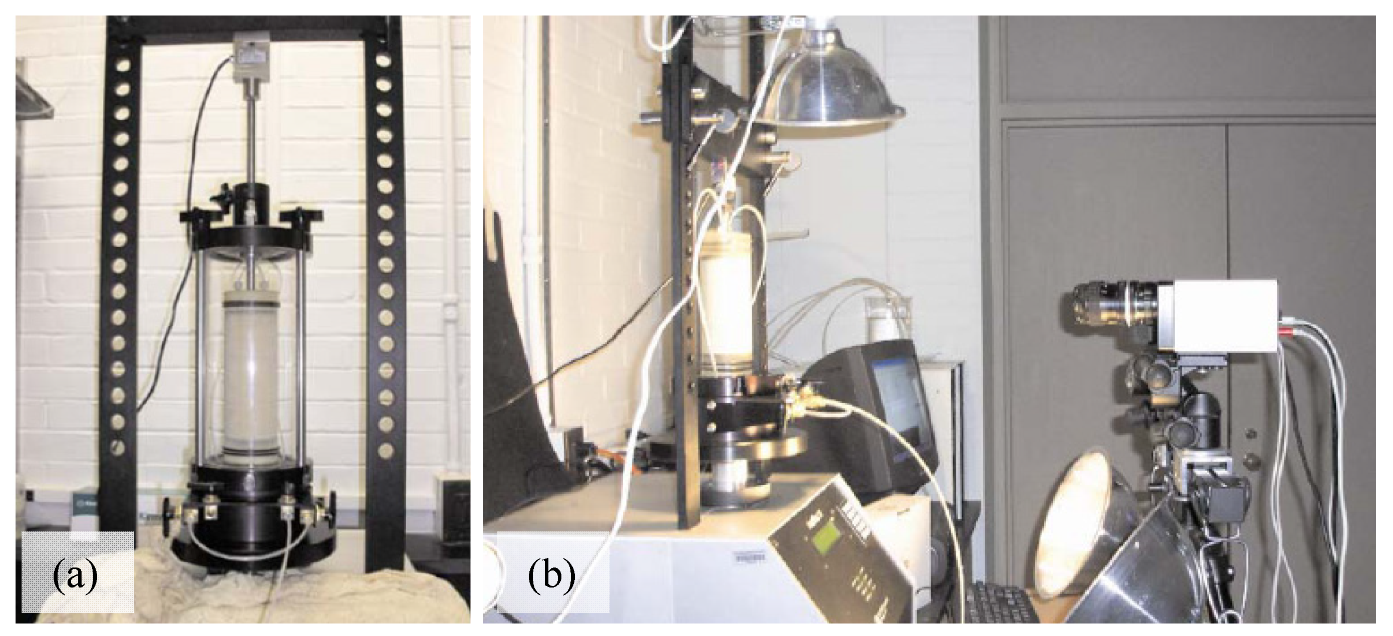
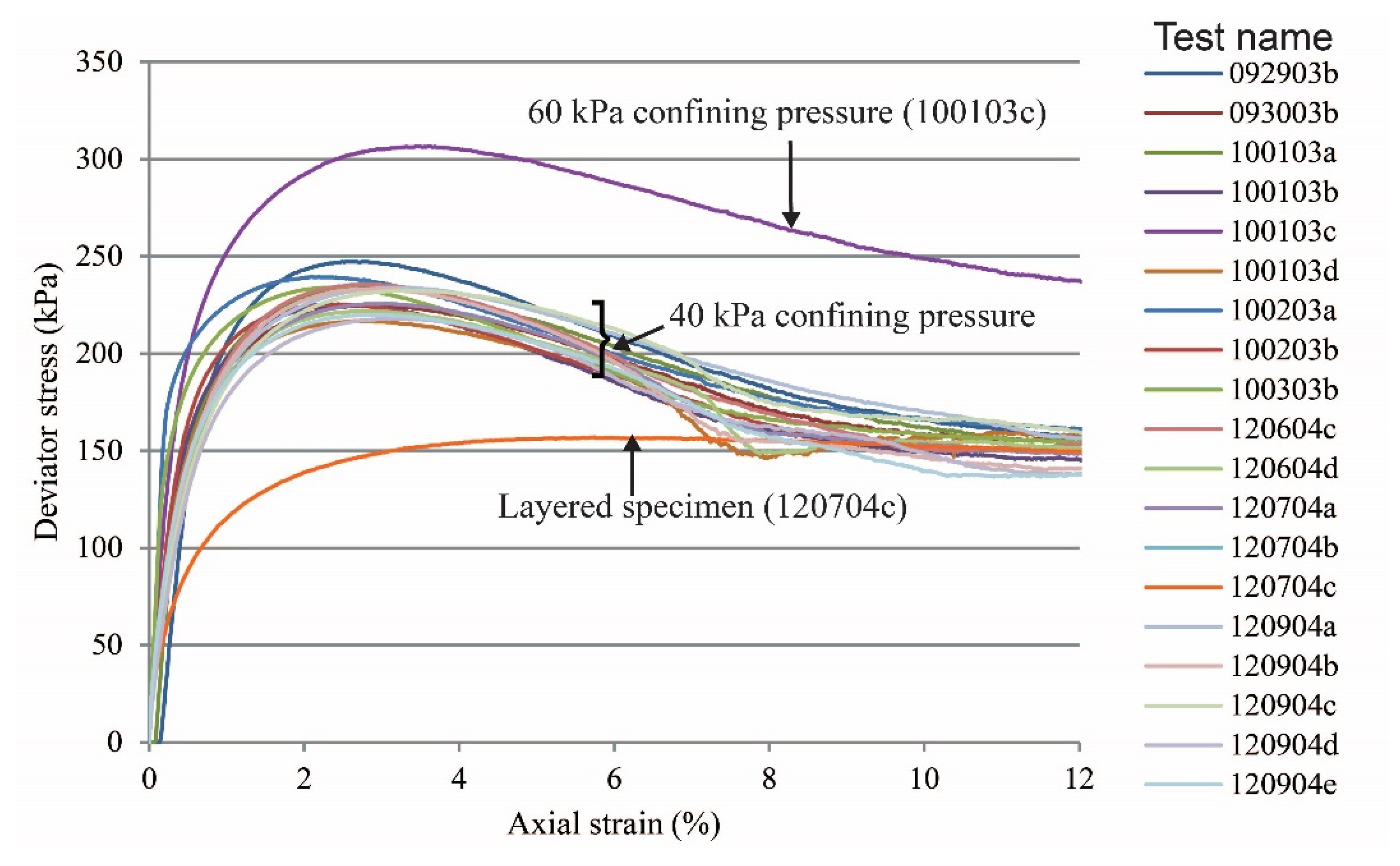
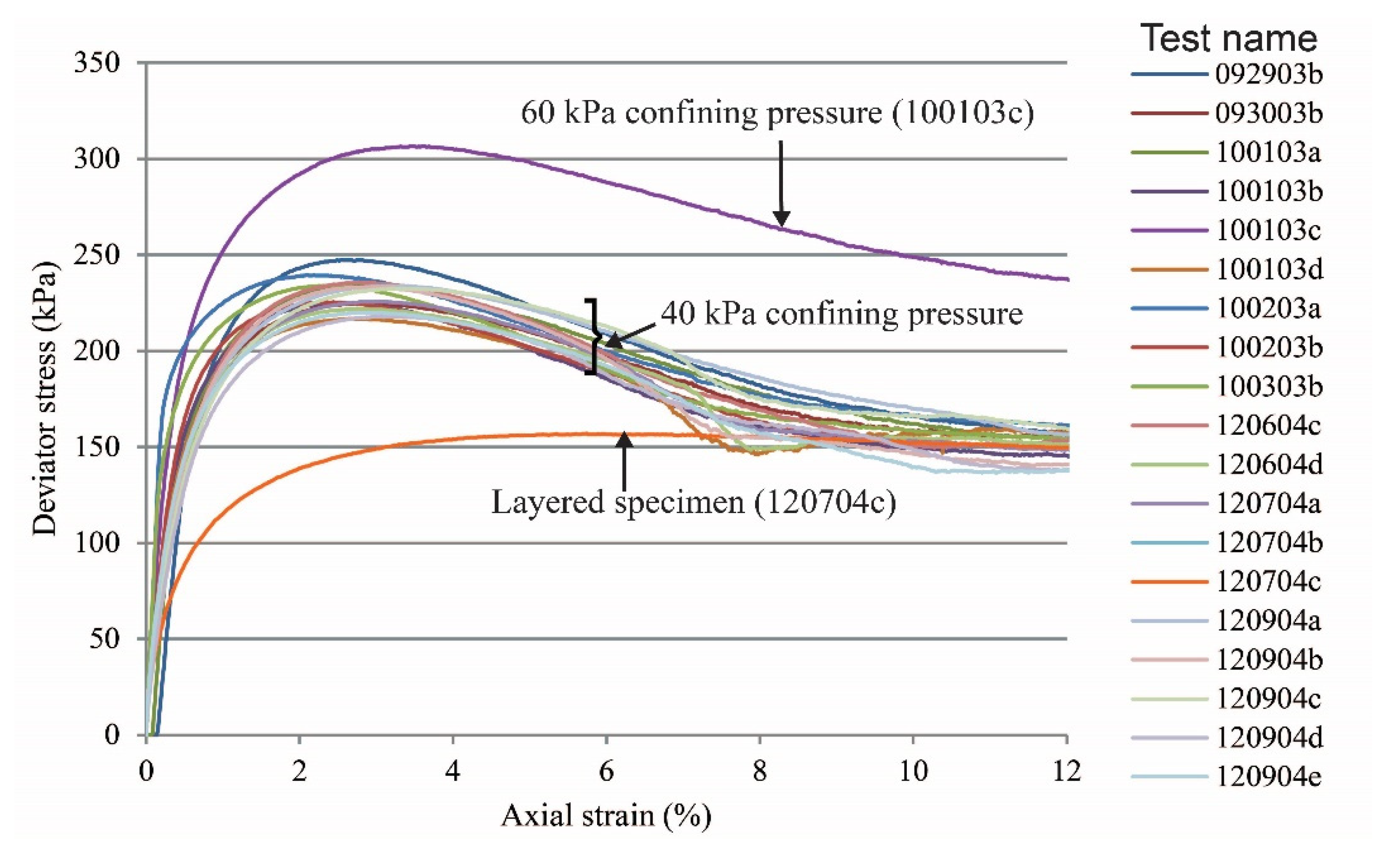
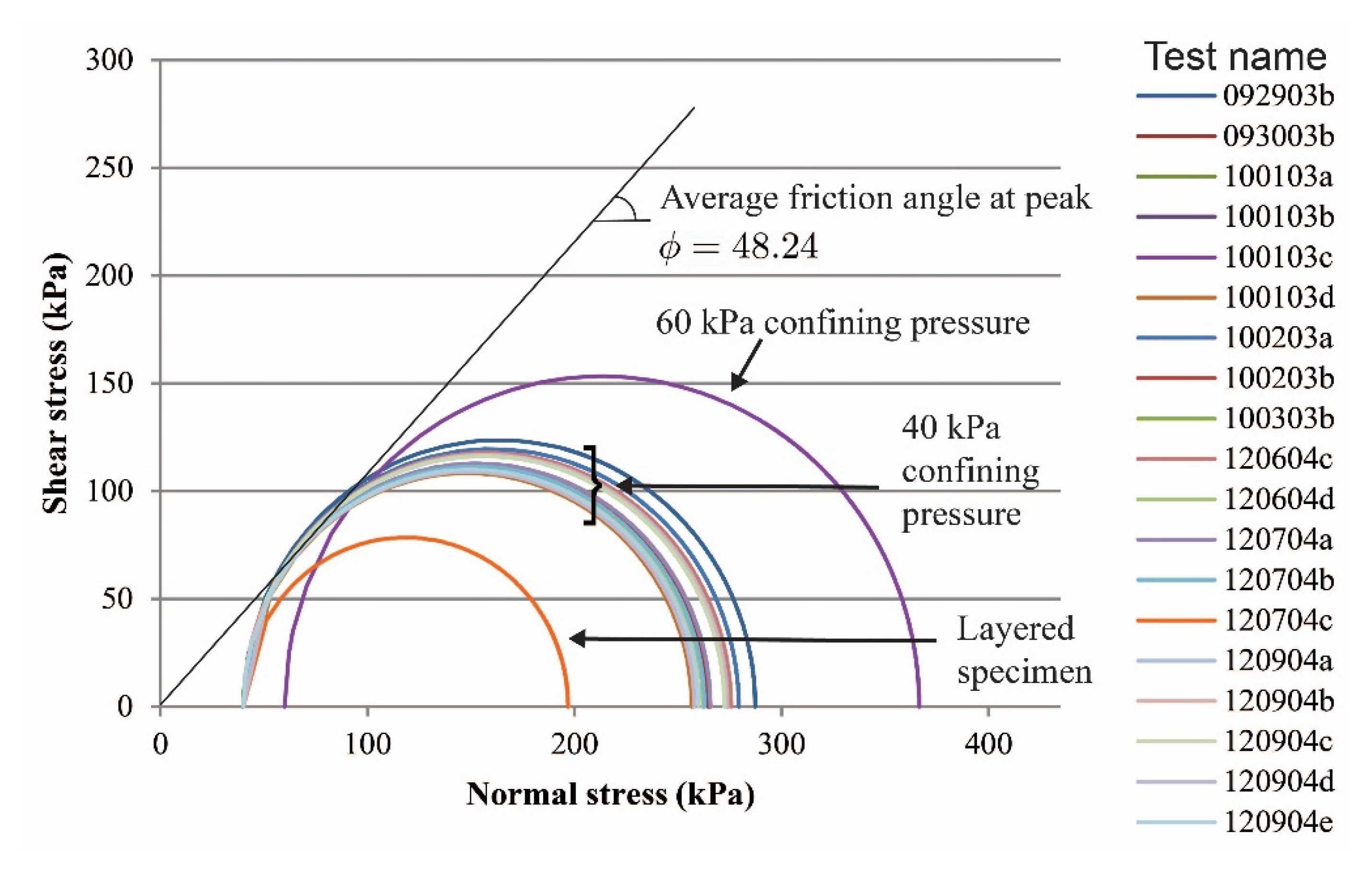
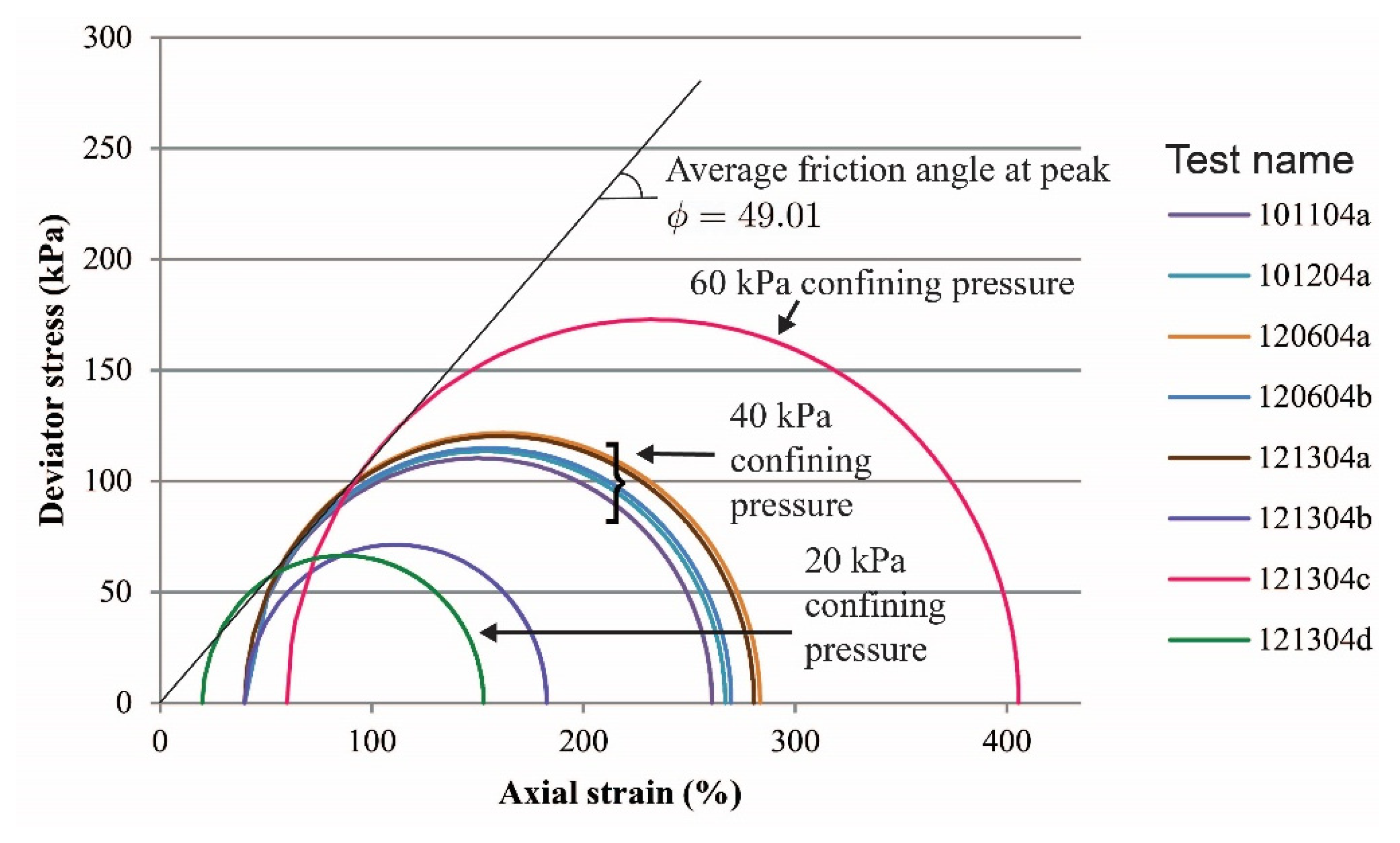
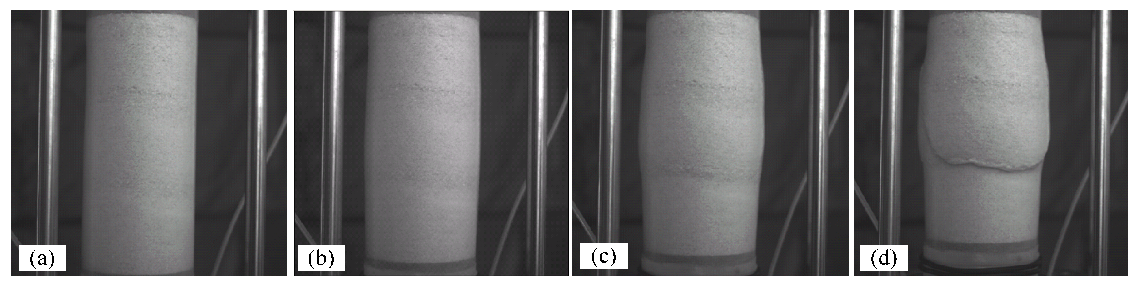
2. Soil Experiments
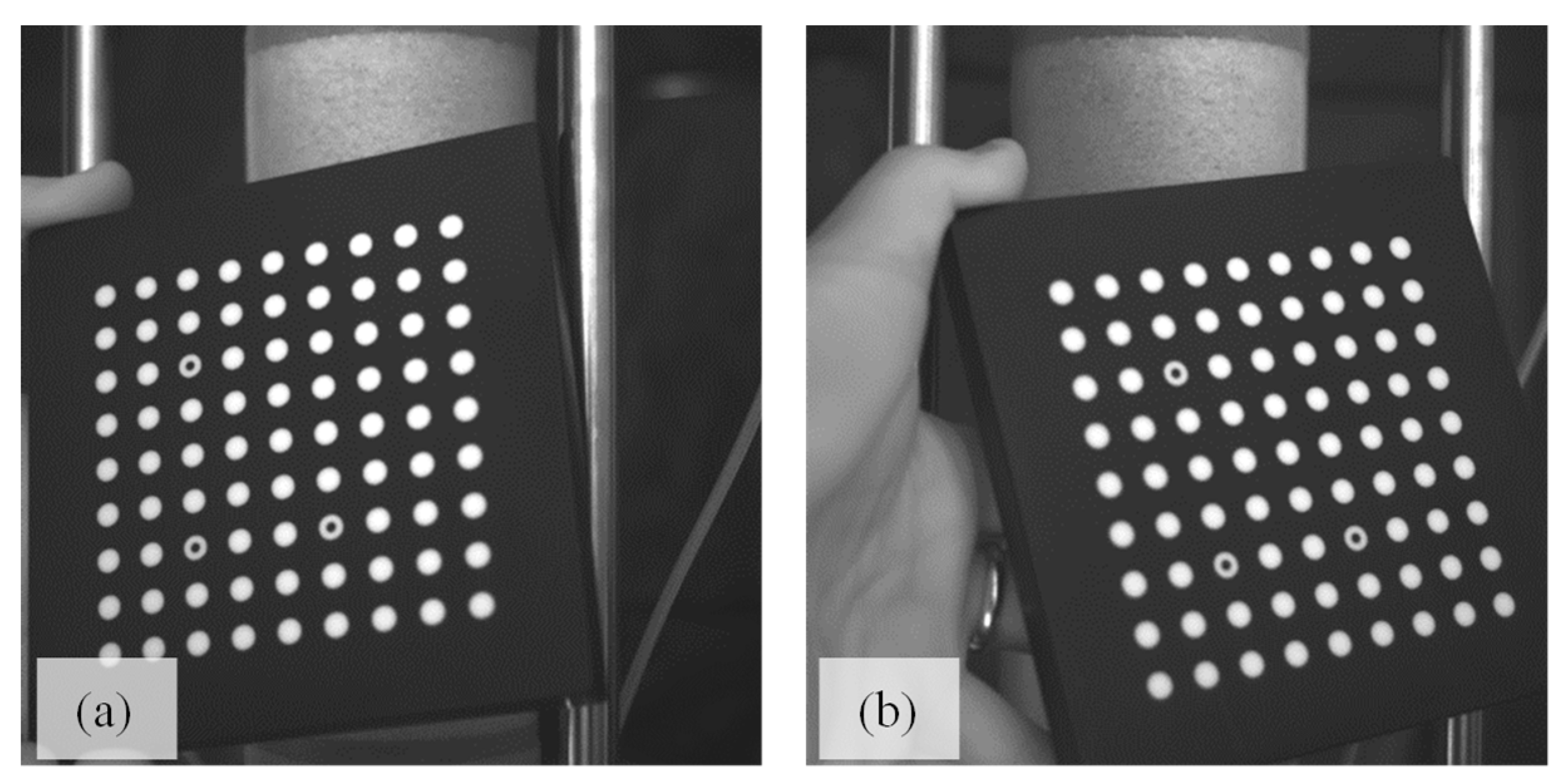
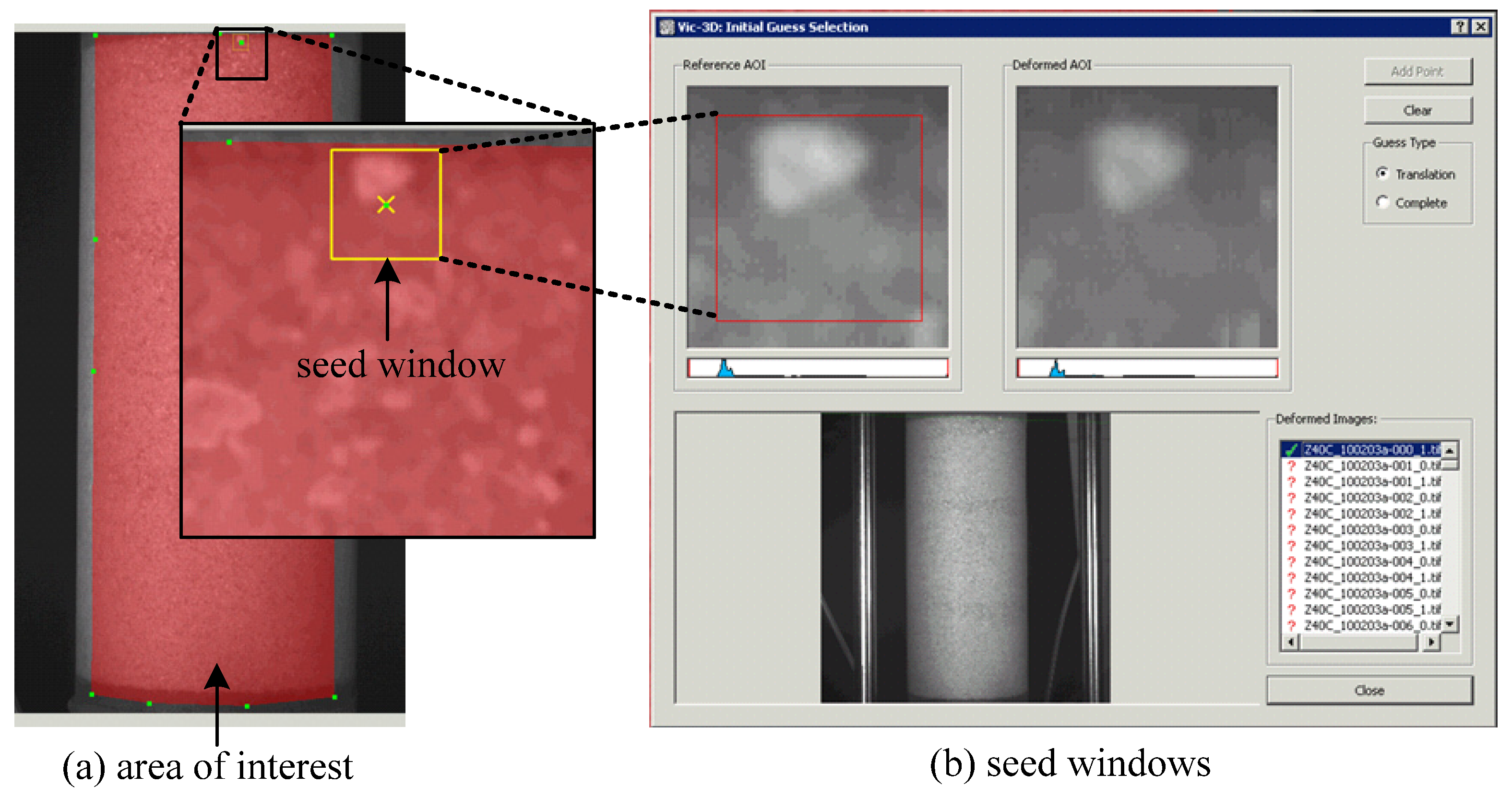
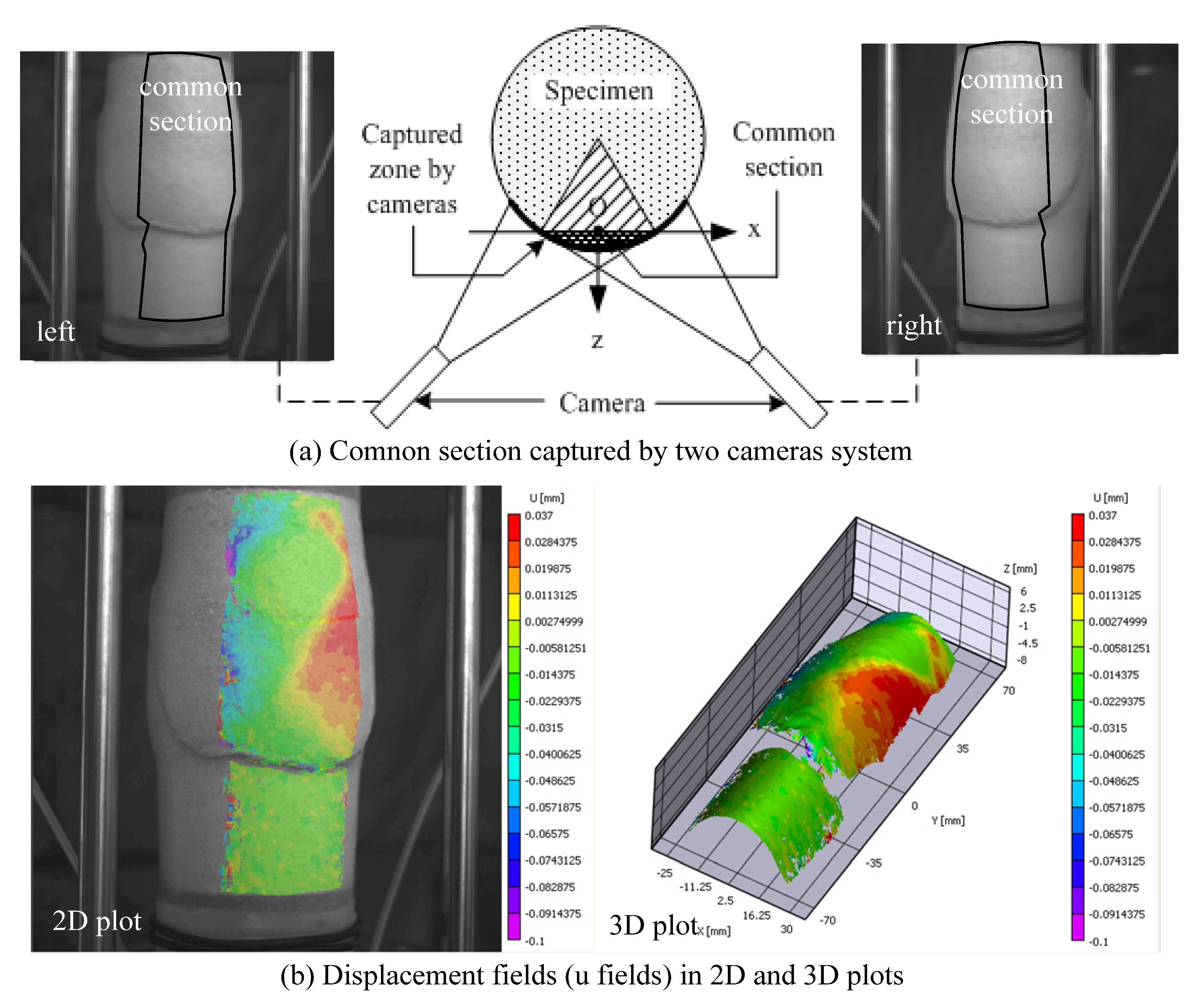
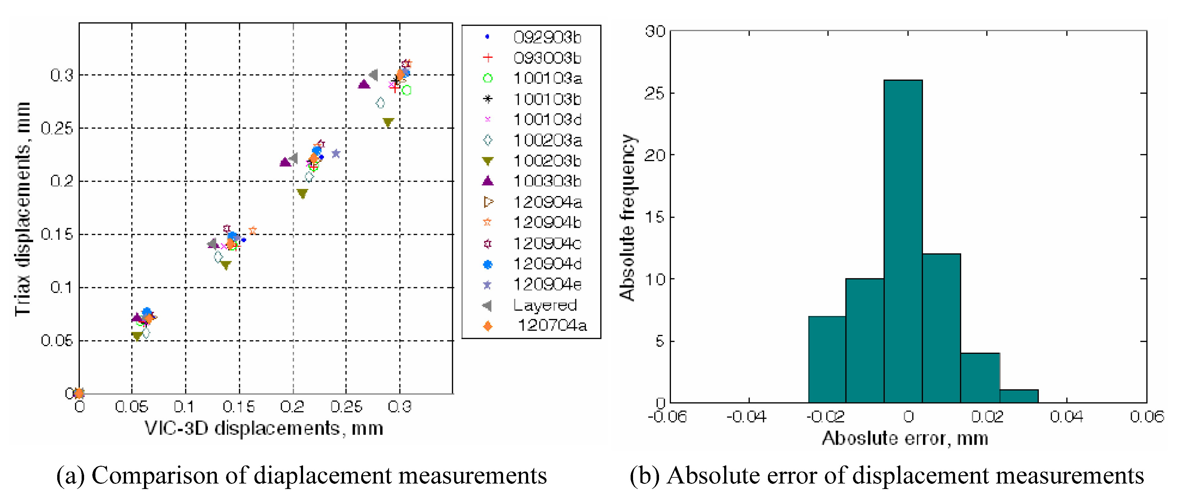
3. 3-D Digital Image Correlation Analysis (3D-DIC)
4. Post-Processing of Image Data
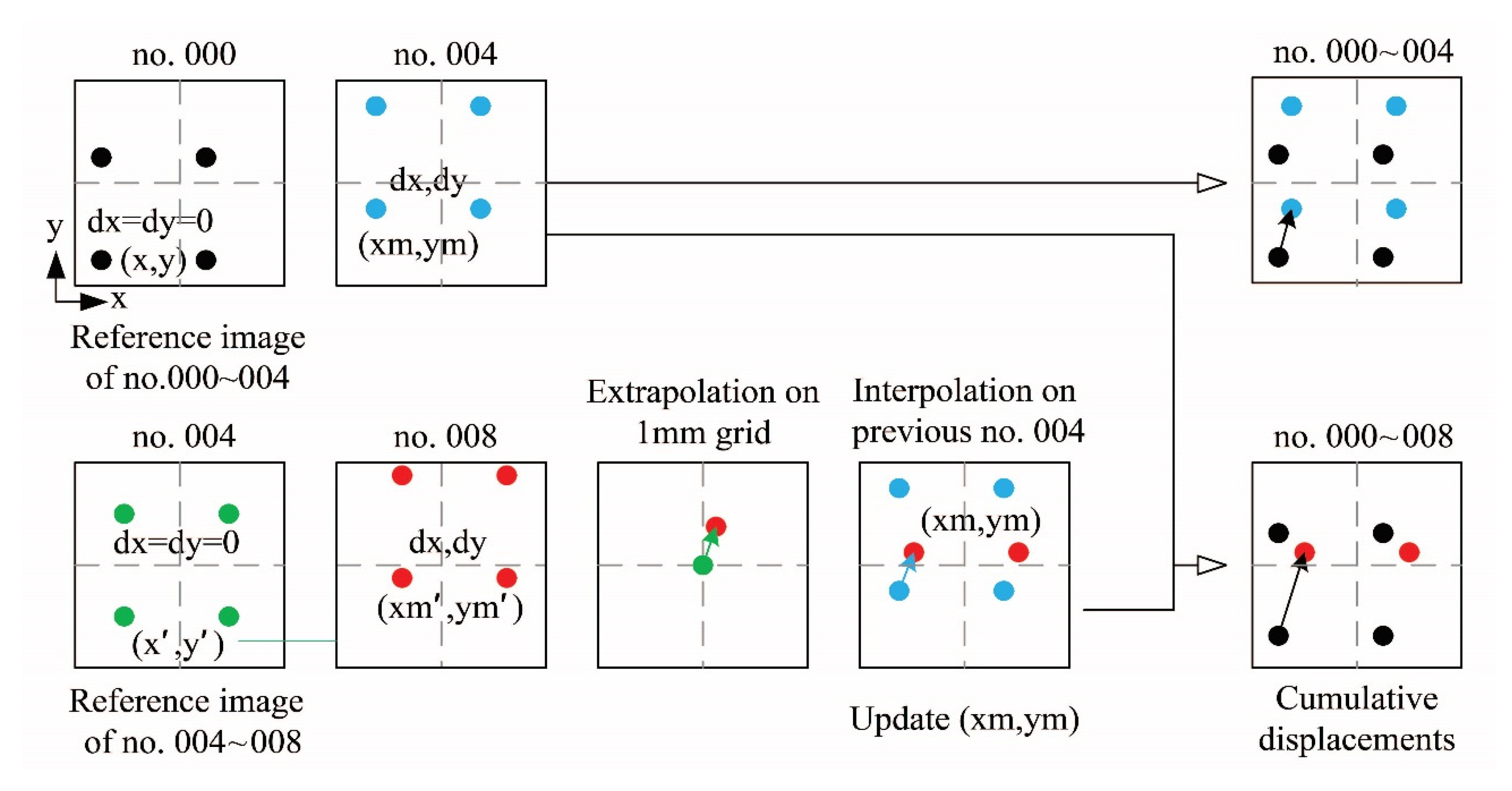
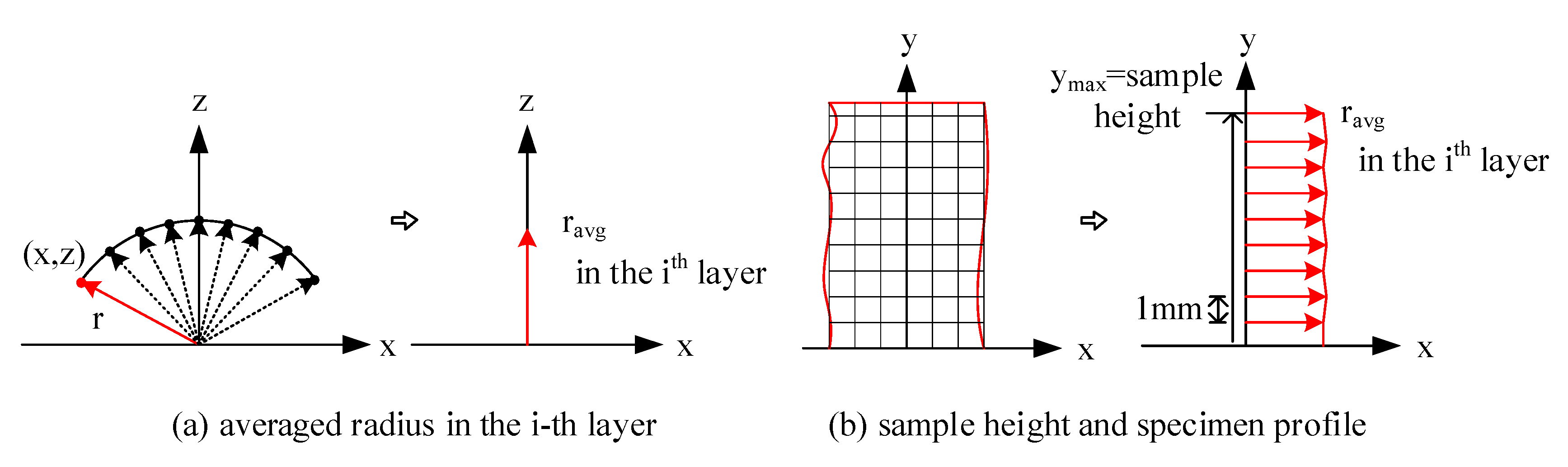
4.1. Piece-Wise Integration of Cumulative Displacement Fields
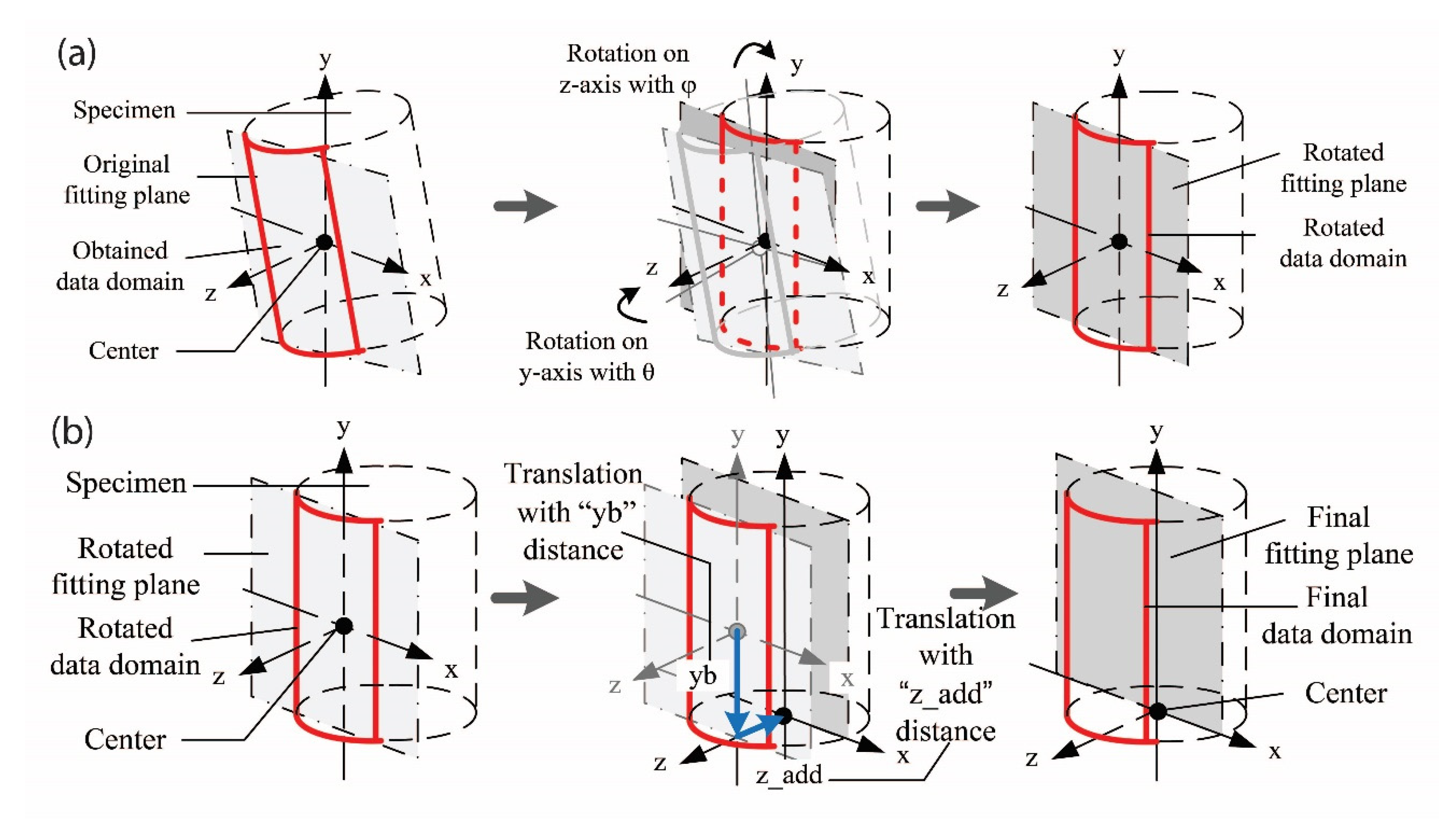
4.2. Geometrical Transformation
5. Results: Displacement Fields
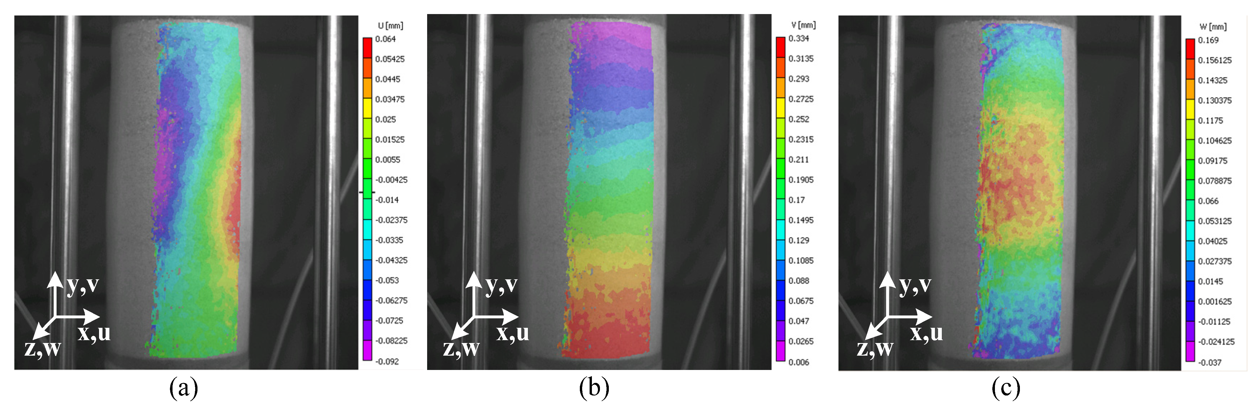
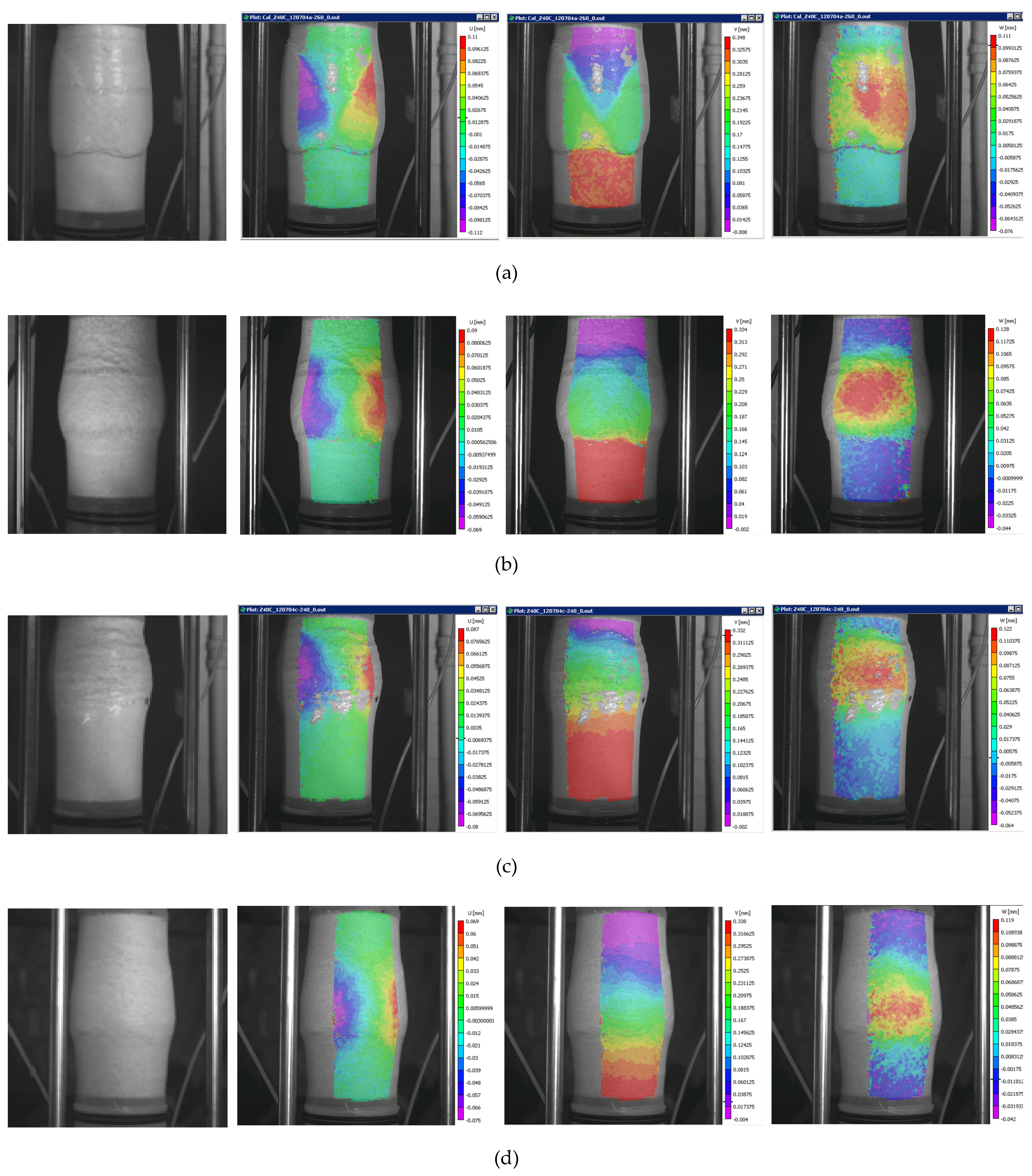
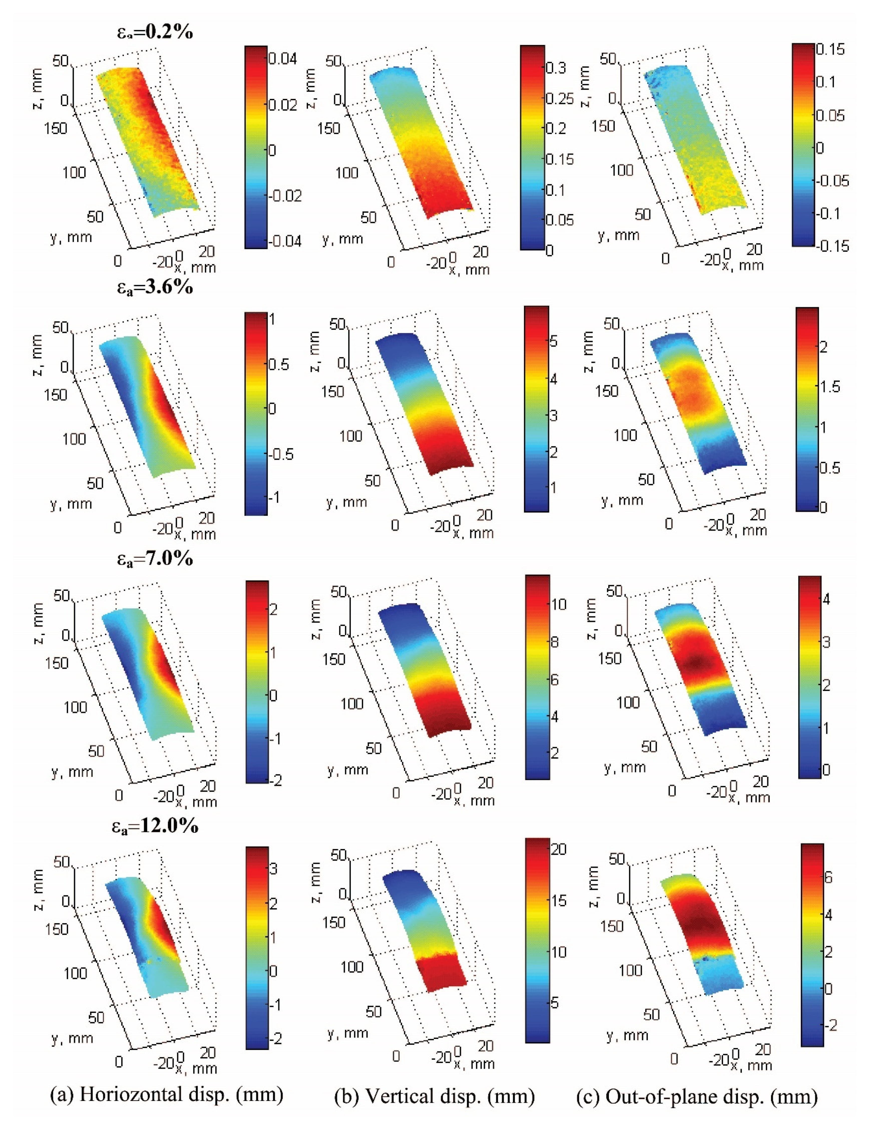
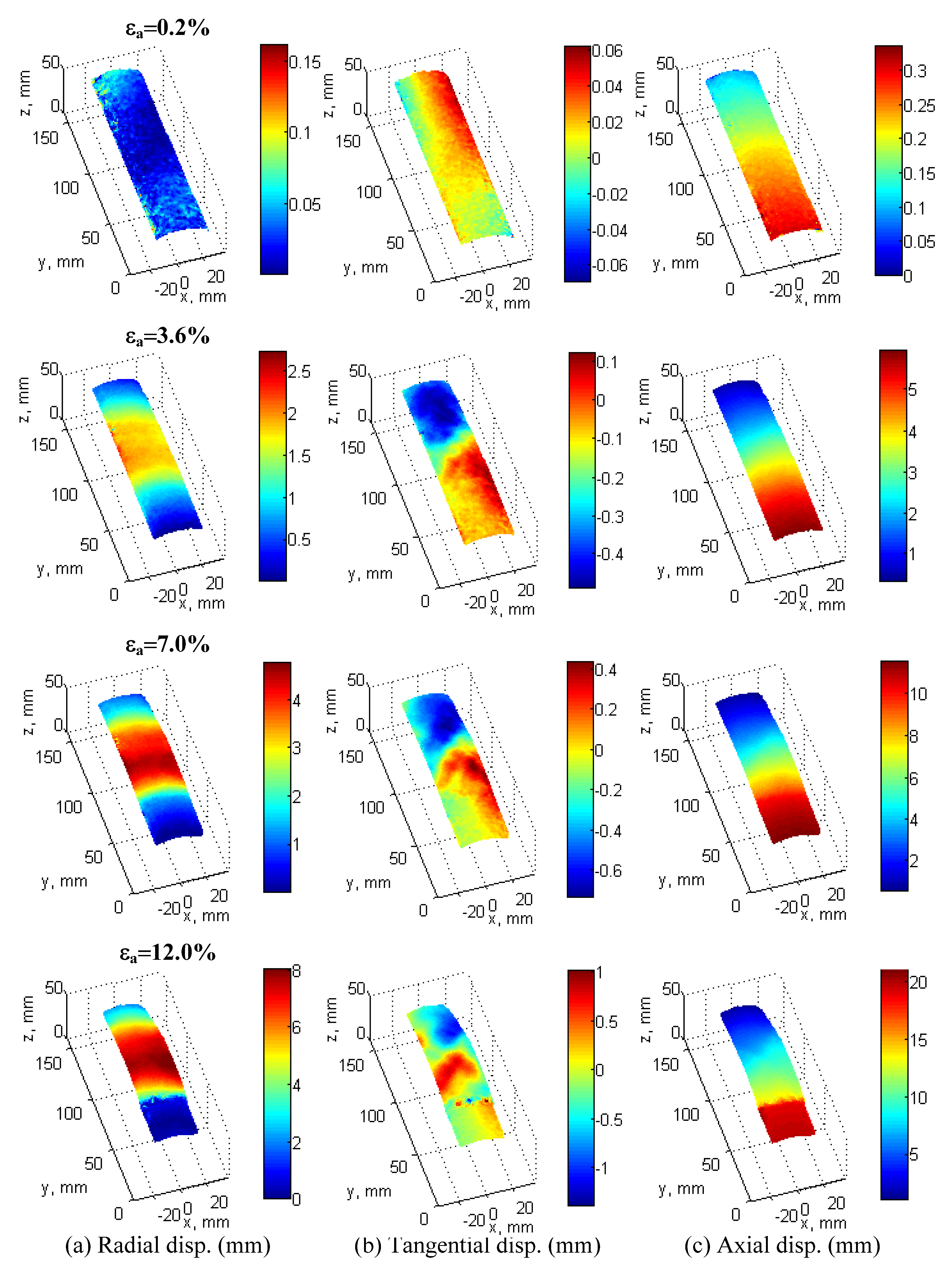
5.1. 3-D Displacement Field under Cartesian and Cylindrical Coordinates
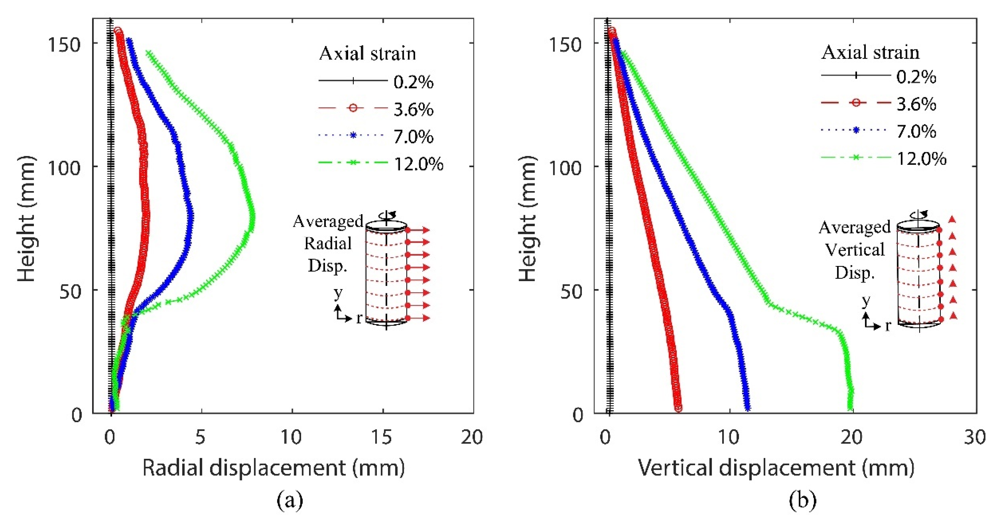
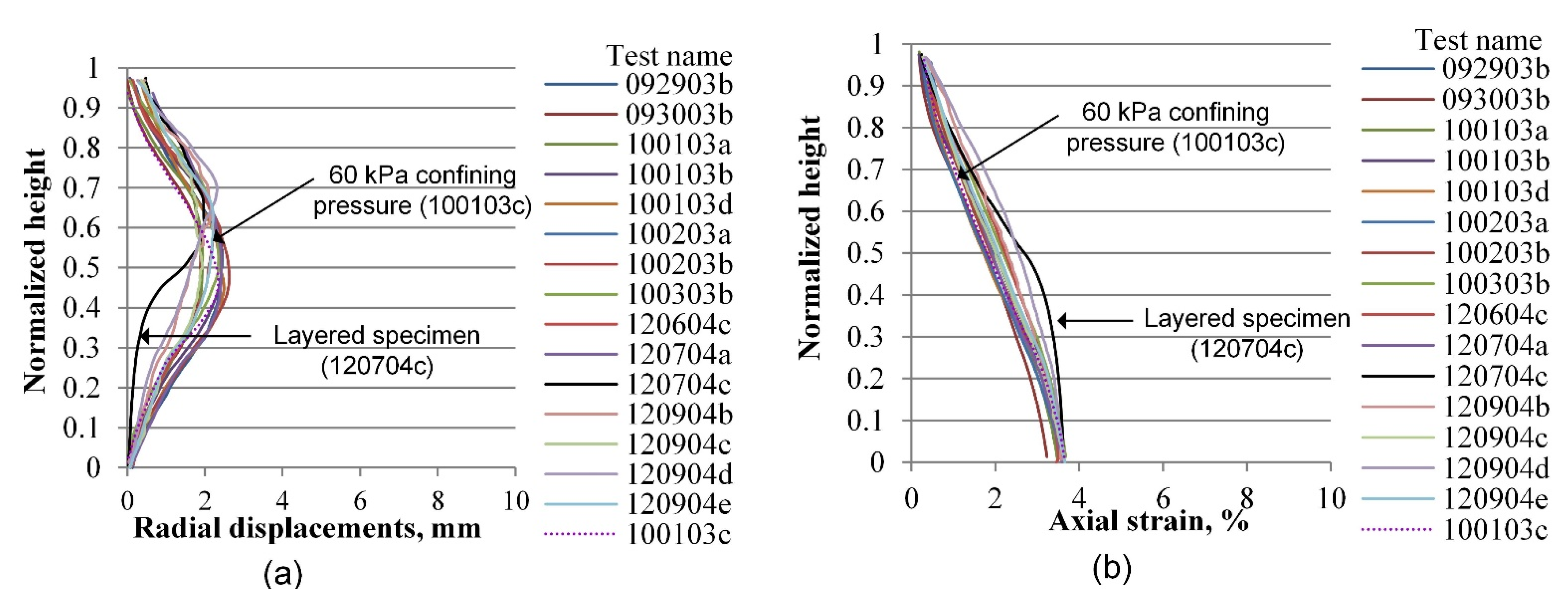
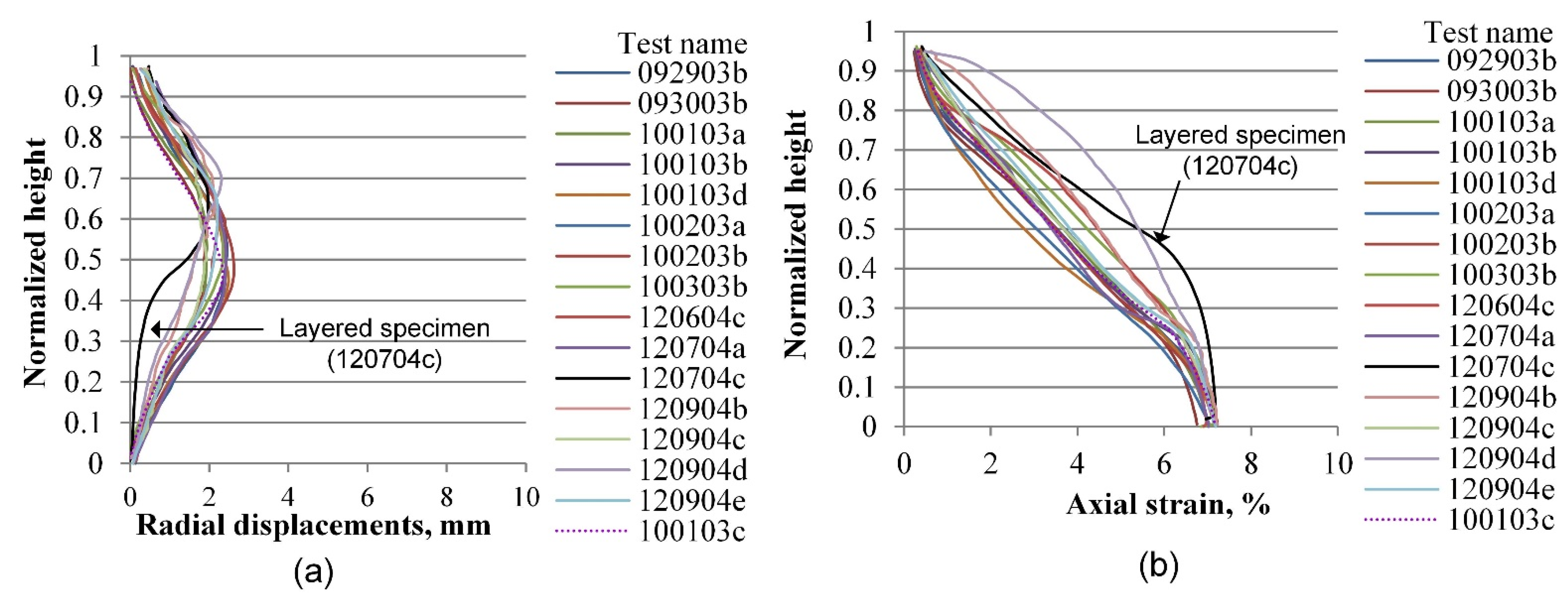
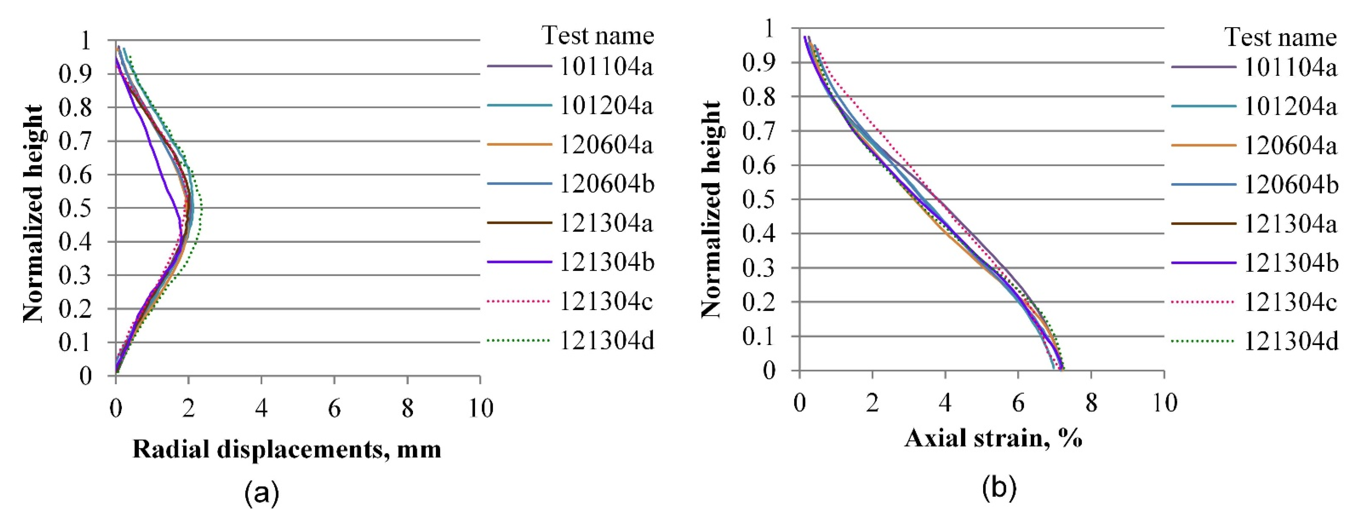
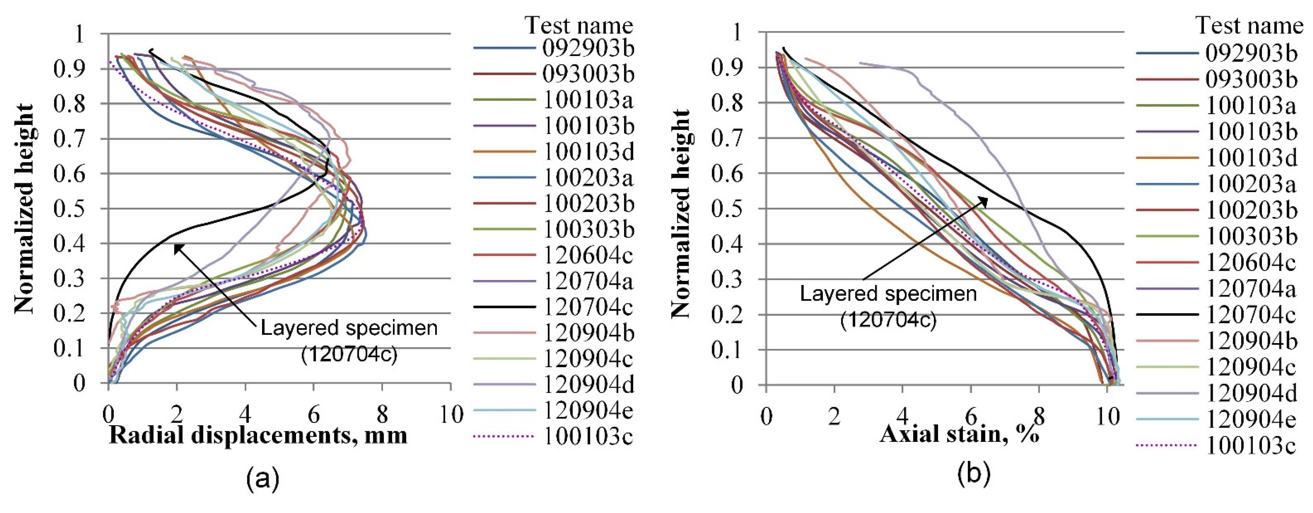
5.2. 1-D Radial and Vertical Displacement Fields (Vertical Profiles)
5.3. Volumetric Strain
6. Conclusions
Supplementary Materials
Author Contributions
Funding
Data Availability Statement
Acknowledgments
Conflicts of Interest
References
- Druckrey, A.M.; Alshibli, K.A.; Al-Raoush, R.I. 3D Characterization of Sand Particle-to-Particle Contact and Morphology. Comput. Geotech. 2016, 74, 26–35. [Google Scholar] [CrossRef] [Green Version]
- Desrues, J.; Andò, E. Strain Localisation in Granular Media. C. R. Phys. 2015, 16, 26–36. [Google Scholar] [CrossRef] [Green Version]
- Roscoe, K.H. The Influence of Strains in Soil Mechanics. Géotechnique 1970, 20, 129–170. [Google Scholar] [CrossRef]
- Desrues, J.; Lanier, J.; Stutz, P. Localization of the Deformation in Tests on Sand Sample. Eng. Fract. Mech. 1985, 21, 909–921. [Google Scholar] [CrossRef]
- Alshibli, K.A.; Sture, S.; Costes, N.C.; Frank, M.; Lankton, M.; Batiste, S.; Swanson, R. Assessment of Localized Deformations in Sand Using X-Ray Computed Tomography. ASTM Geotech. Test. J. 2000, 23, 274–299. [Google Scholar]
- Desrues, J.; Chambon, R.; Mokni, M.; Mazerolle, F. Void Ratio Evolution inside Shear Bands in Triaxial Sand Specimens Studied by Computed Tomography. Géotechnique 1996, 46, 529–546. [Google Scholar] [CrossRef]
- Alshibli, K.A.; Jarrar, M.F.; Druckrey, A.M.; Al-Raoush, R.I. Influence of Particle Morphology on 3D Kinematic Behavior and Strain Localization of Sheared Sand. J. Geotech. Geoenviron. Eng. 2016, 143, 04016097. [Google Scholar] [CrossRef]
- Matsushima, T.; Katagiri, J.; Uesugi, K.; Nakano, T.; Tsuchiyama, A. Micro X-Ray CT at Spring-8 for Granular Mechanics. In Proceedings of the Soil Stress-Strain Behavior: Measurement, Modeling and Analysis; Springer: New York, NY, USA, 2006; pp. 225–234. [Google Scholar]
- Viggiani, G.; Hall, S.A. Full-Field Measurements, a New Tool for Laboratory Experimental Geomechanics. In Proceedings of the Fourth Symposium on Deformation Characteristics of Geomaterials, Atlanta, GA, USA, 21 September 2008; Volume 1, pp. 3–26. [Google Scholar]
- Sutton, M.A.; Orteu, J.J.; Schreier, H. Image Correlation for Shape, Motion and Deformation Measurements-Basic Concepts, Theory and Applications; Springer: New York, NY, USA, 2009. [Google Scholar]
- Khatami, H.; Deng, A.; Jaksa, M. An Experimental Study of the Active Arching Effect in Soil Using the Digital Image Correlation Technique. Comput. Geotech. 2019, 108, 183–196. [Google Scholar] [CrossRef]
- Gedela, R.; Kalla, S.; Sudarsanan, N.; Karpurapu, R. Assessment of Load Distribution Mechanism in Geocell Reinforced Foundation Beds Using the Digital Image Correlation Techniques. Transp. Geotech. 2021, 31, 100664. [Google Scholar] [CrossRef]
- Abedi, S.; Rechenmacher, A.L.; Orlando, A.D. Vortex Formation and Dissolution in Sheared Sands. Granul. Matter 2012, 14, 695–705. [Google Scholar] [CrossRef] [Green Version]
- Omidvar, M.; Chen, Z. (Chris); Iskander, M. Image-Based Lagrangian Analysis of Granular Kinematics. J. Comput. Civ. Eng. 2015, 29, 04014101. [Google Scholar] [CrossRef]
- Rechenmacher, A.; Abedi, S.; Chupin, O. Evolution of Force Chains in Shear Bands in Sands. Géotechnique 2010, 60, 343–351. [Google Scholar] [CrossRef]
- Rechenmacher, A.L.; Abedi, S.; Chupin, O.; Orlando, A.D. Characterization of Mesoscale Instabilities in Localized Granular Shear Using Digital Image Correlation. Acta Geotech. 2011, 6, 205–217. [Google Scholar] [CrossRef] [Green Version]
- Medina-Cetina, Z.; Rechenmacher, A. Influence of Boundary Conditions, Specimen Geometry and Material Heterogeneity on Model Calibration from Triaxial Tests. Int. J. Numer. Anal. Methods Geomech. 2010, 34, 627–643. [Google Scholar] [CrossRef]
- Rechenmacher, A.L.; Medina-cetina, Z. Calibration of Soil Constitutive Models with Spatially Varying Parameters. J. Geotech. Geoenviron. Eng. 2007, 133, 1567–1576. [Google Scholar] [CrossRef]
- Andrade, J.E.; Avila, C.F.; Hall, S.A.; Lenoir, N.; Viggiani, G. Multiscale Modeling and Characterization of Granular Matter: From Grain Kinematics to Continuum Mechanics. J. Mech. Phys. Sol. 2011, 59, 237–250. [Google Scholar] [CrossRef]
- Guo, N.; Zhao, J. 3D Multiscale Modeling of Strain Localization in Granular Media. Comput. Geotech. 2016, 80, 360–372. [Google Scholar] [CrossRef]
- Kawamoto, R.; Andò, E.; Viggiani, G.; Andrade, J.E. All You Need Is Shape: Predicting Shear Banding in Sand with LS-DEM. J. Mech. Phys. Sol. 2018, 111, 375–392. [Google Scholar] [CrossRef] [Green Version]
- Mayo-Corrochano, C.; Sánchez-Aparicio, L.J.; Aira, J.-R.; Sanz-Arauz, D.; Moreno, E.; Pinilla Melo, J. Assessment of the Elastic Properties of High-fired Gypsum Using the Digital Image Correlation Method. Constr. Build. Mater. 2022, 317, 125945. [Google Scholar] [CrossRef]
- Andò, E.; Hall, S.A.; Viggiani, G.; Desrues, J.; Bésuelle, P. Experimental Micromechanics: Grain-Scale Observation of Sand Deformation. Geotech. Lett. 2012, 2, 107–112. [Google Scholar] [CrossRef]
- Medina-Cetina, Z. Probabilistic Calibration of a Soil Model. Ph.D. Thesis, Johns Hopkins University, Baltimore, MD, USA, 2006. [Google Scholar]
- Correlated Solution. Available online: https://www.correlatedsolutions.com/ (accessed on 1 December 2021).
- Desrues, J.; Viggiani, G. Strain Localization in Sand: An Overview of the Experimental Results Obtained in Grenoble Using Stereophotogrammetry. Int. J. Numer. Anal. Methods Geomech. 2004, 28, 279–321. [Google Scholar] [CrossRef]
- Chupin, O.; Rechenmacher, A.L.; Abedi, S. Finite Strain Analysis of Nonuniform Deformation inside Shear Bands in Sands. Int. J. Numer. Anal. Methods Geomech. 2012, 36, 1651–1666. [Google Scholar] [CrossRef] [Green Version]
- Sutton, M.A.; Yan, J.H.; Tiwari, V.; Schreier, H.W.; Orteu, J.J. The Effect of Out-of-Plane Motion on 2D and 3D Digital Image Correlation Measurements. Opt. Lasers Eng. 2008, 46, 746–757. [Google Scholar] [CrossRef] [Green Version]
- Lava, P.; Coppieters, S.; Wang, Y.; van Houtte, P.; Debruyne, D. Error Estimation in Measuring Strain Fields with DIC on Planar Sheet Metal Specimens with a Non-Perpendicular Camera Alignment. Opt. Lasers Eng. 2011, 49, 57–65. [Google Scholar] [CrossRef]
- Song, A. Deformation Analysis of Sand Specimens Using 3D Digital Image Correlation for the Calibration of an Elasto-Plastic Model. Ph.D. Thesis, Texas A&M University, College Station, TX, USA, 2012. [Google Scholar]
- Macari, E.; Parker, J.; Costes, N. Measurement of Volume Changes in Triaxial Tests Using Digital Imaging Techniques. Geotech. Test. J. 1997, 20, 103–109. [Google Scholar] [CrossRef]


| Test No. | Test Name | Height (mm) | Diameter (mm) | Initial Density (kg/m3) | Relative Density (%) | Confinement (kPa) | Notes |
|---|---|---|---|---|---|---|---|
| 1 | 092903b | 155.50 | 71.33 | 1710.95 | 91.09 | 40 | - |
| 2 | 093003b | 156.67 | 71.41 | 1696.00 | 85.96 | 40 | - |
| 3 | 100103a | 157.67 | 71.29 | 1702.22 | 88.10 | 40 | - |
| 4 | 100103b | 155.83 | 71.24 | 1717.13 | 93.18 | 40 | - |
| 5 | 100103c | 157.67 | 71.54 | 1703.87 | 88.67 | 60 | - |
| 6 | 100103d | 154.33 | 70.86 | 1702.41 | 88.17 | 40 | - |
| 7 | 100203a | 157.50 | 71.45 | 1715.32 | 92.57 | 40 | - |
| 8 | 100203b | 155.00 | 71.48 | 1711.91 | 91.41 | 40 | - |
| 9 | 100303b | 158.17 | 71.29 | 1718.70 | 93.71 | 40 | - |
| 14 | 120604c | 158.83 | 70.72 | 1717.48 | 93.30 | 40 | Light reflection |
| 15 | 120604d | 158.83 | 70.84 | 1716.99 | 93.13 | 40 | Light reflection |
| 16 | 120704a | 158.83 | 71.37 | 1708.07 | 90.11 | 40 | Light reflection |
| 17 | 120704b | 159.00 | 71.30 | 1686.96 | 82.82 | 40 | Light reflection |
| 18 | 120704c | 157.67 | Average: 70.88 | Average: 1648.06 | Average: 68.90 | 40 | Layered specimen |
| 79.50 | 71.27 | 1734.17 | 98.87 | 40 | Lower: dense sand | ||
| 78.17 | 70.68 | 1549.61 | 30.54 | 40 | Upper: loose sand | ||
| 19 | 120904a | 158.67 | 71.15 | 1707.72 | 89.99 | 40 | Light reflection |
| 20 | 120904b | 160.00 | 70.98 | 1720.40 | 94.28 | 40 | - |
| 21 | 120904c | 159.67 | 71.11 | 1713.13 | 91.83 | 40 | - |
| 22 | 120904d | 159.00 | 71.13 | 1707.89 | 90.04 | 40 | - |
| 23 | 120904e | 160.00 | 70.99 | 1718.70 | 93.71 | 40 | - |
| Test No. | Test Name | Height (mm) | Diameter (mm) | Initial Density (kg/m3) | Relative Density (%) | Confinement (kPa) | Notes |
|---|---|---|---|---|---|---|---|
| 10 | 101104a | 159.33 | 70.87 | 1724.89 | 95.79 | 40 | Light reflection |
| 11 | 101204a | 160.00 | 71.46 | 1708.03 | 90.09 | 40 | - |
| 12 | 120604a | 159.33 | 71.31 | 1721.06 | 94.50 | 40 | Light reflection |
| 13 | 120604b | 159.33 | 70.94 | 1715.13 | 92.50 | 40 | Light reflection |
| 24 | 121304a | 160.00 | 71.30 | 1721.73 | 94.73 | 40 | - |
| 25 | 121304b | 158.17 | 70.86 | 1588.84 | 46.39 | 40 | Loose specimen |
| 26 | 121304c | 160.00 | 70.48 | 1718.72 | 93.72 | 60 | - |
| 27 | 121304d | 159.50 | 71.38 | 1736.71 | 99.71 | 20 | - |
Publisher’s Note: MDPI stays neutral with regard to jurisdictional claims in published maps and institutional affiliations. |
© 2022 by the authors. Licensee MDPI, Basel, Switzerland. This article is an open access article distributed under the terms and conditions of the Creative Commons Attribution (CC BY) license (https://creativecommons.org/licenses/by/4.0/).
Share and Cite
Medina-Cetina, Z.; Song, A.; Zhu, Y.; Pineda-Contreras, A.R.; Rechenmacher, A. Global and Local Deformation Effects of Dry Vacuum-Consolidated Triaxial Compression Tests on Sand Specimens: Making a Database Available for the Calibration and Development of Forward Models. Materials 2022, 15, 1528. https://doi.org/10.3390/ma15041528
Medina-Cetina Z, Song A, Zhu Y, Pineda-Contreras AR, Rechenmacher A. Global and Local Deformation Effects of Dry Vacuum-Consolidated Triaxial Compression Tests on Sand Specimens: Making a Database Available for the Calibration and Development of Forward Models. Materials. 2022; 15(4):1528. https://doi.org/10.3390/ma15041528
Chicago/Turabian StyleMedina-Cetina, Zenon, Ahran Song, Yichuan Zhu, Alma Rosa Pineda-Contreras, and Amy Rechenmacher. 2022. "Global and Local Deformation Effects of Dry Vacuum-Consolidated Triaxial Compression Tests on Sand Specimens: Making a Database Available for the Calibration and Development of Forward Models" Materials 15, no. 4: 1528. https://doi.org/10.3390/ma15041528