Article

An ECMS Based on Model Prediction Control for Series Hybrid Electric Mine Trucks

1
Jiangsu XCMG Research Institute Co., Ltd., Xuzhou 221004, China
2
School of Materials and Physics, China University of Mining and Technology, Xuzhou 221116, China
*
Author to whom correspondence should be addressed.
Energies 2023, 16(9), 3942; https://doi.org/10.3390/en16093942
Submission received: 10 April 2023 / Revised: 30 April 2023 / Accepted: 5 May 2023 / Published: 7 May 2023
(This article belongs to the Special Issue Energy Management Strategies for Battery and Hybrid Electric Vehicles)

Abstract

:
This paper presents an equivalent consumption minimization strategy (ECMS) based on model predictive control for series hybrid electric mine trucks (SHE-MTs), the objective of which is to minimize fuel consumption. Two critical works are presented to achieve the goal. Firstly, to gain the real-time speed trajectory on-line, a speed prediction model is established by utilizing a recurrent neural network (RNN). Specifically, a hybrid optimization algorithm based on the genetic algorithm (GA) and the particle swarm optimization algorithm (PSOA) is used to enhance the prediction precision of the speed prediction model. Then, on this basis, an ECMS based on MPC (ECMS-MPC) is proposed. In this process, to improve the real-time and working condition adaptability of the ECMS-MPC, the power-optimal fuel consumption mapping model of the range extender is established, and the equivalent factor (EF) is real-time adjusted by means of the PSOA. Finally, taking a cement mining road as the research object, the proposed strategy is simulated with the collected actual vehicle data. The experimental results indicate that the prediction precision of the proposed speed prediction model is over 98%, realizing on-line speed prediction effectively. Furthermore, compared to the existing real-time EMSs, its fuel-saving rate had an increase of more than 13%. This indicates that the designed ECMS-MPC is able to offer a novel and effective method for the on-line energy management of the SHE-MTs.

1. Introduction

Under the traction of the double carbon policy, series hybrid electric mine trucks (SHE-MTs) have become one of the important ways to realize the green and sustainable development of mine trucks [1,2]. To make full use of the fuel-saving and emission-reducing performance of the SHE-MTs, it is very essential to adopt appropriate energy management strategies (EMSs) to allocate the output power of the range extender and battery [3,4]. At present, the existing EMSs are capable of dividing into the following main categories: rule-based (RB) EMSs and optimization-based EMSs [5].
RB EMSs [6,7,8,9] mainly include charge-depleting and charge-sustaining (CDCS) [6], deterministic RB (DRB) [7], and fuzzy RB (FRB) [8] EMSs, which are primitively presented on-line EMSs. In general, RB EMSs can quickly match the corresponding rules in accordance with the driving conditions, possessing excellent real-time and implementation performance. In [10], a tunable RB EMS was proposed by means of adjusting the mixed weight factor. On the basis of this, the engine operating state could be dynamically adjusted, and the optimal operation points of the engine were chosen in accordance with its map. Lastly, it achieved fuel savings of 18.9% in comparison to the hydrostatic loader. Zhao et al. [11] proposed a fuzzy logic control strategy, taking the demand torque and state of charge (SoC) of the supercapacitor as inputs, and outputting the torque of the engine and motor as outputs. Finally, compared to the conventional loader, the strategy could decrease fuel consumption by about 16.6%. Nevertheless, the fuel-saving performance of RB EMSs not only relies on experts’ experience but also is constrained by the fixed parameters of the rule base, resulting in poor fuel-saving robustness and driving condition adaptability. Therefore, many scholars have proposed optimization-based EMSs, mainly containing global and instantaneous optimization EMSs [12]. Among them, the global optimization EMSs can realize the globally optimal solution of the fuel consumption when the priori information (speed, acceleration, slope angle, etc.) of the driving cycle is known [13,14]. However, in terms of SHE-MTs, the priori information of the driving cycle is difficult to be accurately obtained in advance in practical situations. In addition, global optimization EMSs, with a large amount of calculation, can only be used for offline optimization and are not suitable for on-line energy management.
In contrast, instantaneous optimization EMSs are capable of achieving fuel consumption optimization instantly or in a short duration, which mainly contain the equivalent consumption minimization strategy (ECMS) [15,16,17,18], model predictive control (MPC) EMSs [19,20,21,22], and intelligent control EMSs [23,24,25]. The critical principle of the ECMS [15] is to transform the global optimization problem into an instantaneous optimization problem that minimizes the real-time equivalent fuel consumption by adjusting an equivalent factor (EF) at each moment [18,26]. The references [15,16] utilized the ECMS optimization idea to achieve real-time on-line energy management. The multi-objective overall optimization method was used to improve the ECMS [17]. However, in terms of the random driving states and complex working conditions of SHE-MTs, it is very difficult to correctively obtain the future driving condition information in advance. In this case, the ECMS is not able to obtain the optimally instantaneous equivalent fuel consumption at every time according to the unchanging fuel–electricity EF. For this reason, to make the ECMS adapt to complex and time-varying working conditions, Zhang et al. [18] and Sun et al. [26] respectively proposed a driving-condition recognition-based adaptive ECMS, which can adjust the EF on-line according to the changes in the working condition. In [27], the EF boundary of the ECMS was studied by means of the Hamilton equation of Pontryagin’s minimum principle (PMP). On this basis, a novel fusion-adaptive ECMS was proposed, which was more suitable for on-line applications. Gu et al. [28] developed an optimized ECMS, the EF of which was adjusted by considering the identification of the driving pattern information. In [29,30], adaptive adjustment of the optimal EF on the basis of the proportional integral controller was described regarding the reference SoC error and its feedback. Although the ECMS has the advantage of instantaneous optimization, its energy consumption optimization effect is limited because of not considering the global or local information of future driving conditions.
Different from the ECMS, MPC [31] EMSs and intelligent control [32] EMSs solve the energy consumption optimization problem by taking into account the future state information. Among them, the optimization target of MPC EMSs is to obtain a real-time optimal control strategy by minimizing the local energy consumption of the preview window [19,33]. In order to achieve the goal, the driving information of the preview window is necessary to be predicted by MPC EMSs first. Then, on the basis of this, the optimization algorithms [13] are utilized to compute the optimal control strategy on-line. As the vehicle continues to drive, the predicted condition information continuously updates. Meanwhile, the optimal control sequence is obtained by rolling optimization in the prediction time horizon. Liu et al. [14] proposed a dynamic programming (DP)-based MPC EMS, further reducing the fuel consumption and emissions of the vehicle. Han et al. [20] presented an MPC EMS based on PMP to reduce operating costs while assuring that the electromagnetic temperature is lower than the limit value, achieving real-time energy management. In [21], taking the hybrid loader as the research object, a predictive control strategy on the basis of stochastic DP was proposed. Contrasting with non-predictive EMSs, it could save fuel consumption by about 5%. However, the calculation amounts for the DP and PMP algorithms also increase with the increase in the preview window size, and the solution of the PMP covariate variable is difficult, making them not suitable for real-time optimization. The references [22,34] described stochastic predictive control EMSs based on the Markov Chain according to the driving behavior of the driver. Vadamalu et al. [35] presented an MPC EMS utilizing the Markov Chain. In this strategy, an explicit MPC algorithm was used to solve the constrained energy consumption optimization problem. However, the probability transfer matrices of the Markov Chain increased faster as the driving time became longer, causing a larger computational burden and bad on-line performance of the EMS. For this purpose, intelligent control [32] EMSs were proposed, which solved the energy consumption optimization problem by reinforcement learning (RL), avoiding the computing burden, and having better on-line application potential. In [23], an EMS based on a deep Q-learning algorithm was proposed, which had less training time and faster convergence speed than the general Q-learning strategy, without reducing the optimization effect. Liu et al. [24] proposed a heuristic planning EMS based on dynamic RL, which can overcome the computational burden of the general Q-learning algorithms and the probability transition matrices of the Markov decision process. Wu et al. [25] proposed an EMS based on depth RL, which used a depth gradient algorithm to conduct parameter learning, and its energy optimization effect was better than the discrete Q-learning strategy. However, the optimization effect of the intelligent control EMSs depends on the experience knowledge and learning methods of the parameters and completeness of the sample data, restricting its on-line application.
To further reduce the algorithm computational amount and improve the working condition adaptability of the above on-line EMSs, this paper fully integrates the advantages of the ECMS instantaneous optimization and MPC rolling optimization, designing a novel ECMS based on MPC (ECMS-MPC). Compared to the existing on-line EMSs, the proposed EMS can realize better real-time performance and condition adaptability, with strong fuel-saving robustness.
For achieving the above objectives, the contributions in this paper are as follows. First, to achieve the real-time speed trajectory on-line, a speed prediction model is built using a recurrent neural network (RNN) [36,37,38]. Specifically, the hybrid optimization method of the genetic algorithm (GA) [39,40] and particle swarm optimization algorithm (PSOA) [41] are utilized to optimize the initial parameters of the prediction model to enhance the speed prediction precision of the model. Then, an ECMS-MPC is proposed. In this process, to improve the calculation speed and real-time performance of the proposed EMS, the power-optimal fuel consumption mapping model of the range extender is established. In addition, to further improve the adaptability to random conditions of the SHE-MT, the EF is real-time adjusted by means of the PSOA [41]. Lastly, simulation research is carried out for using the designed ECMS-MPC on a practical cement mine road.
The structures of the paper are as follows. The SHE-MT model and the fuel consumption optimization problem are described in Section 2. Section 3 establishes the speed prediction model. The ECMS-MPC is described in Section 4. Next, the speed prediction effect and the ECMS-MPC performance are discussed and analyzed in Section 5. Lastly, the conclusions and prospects are given in Section 6.

2. Problem Description and Formulation
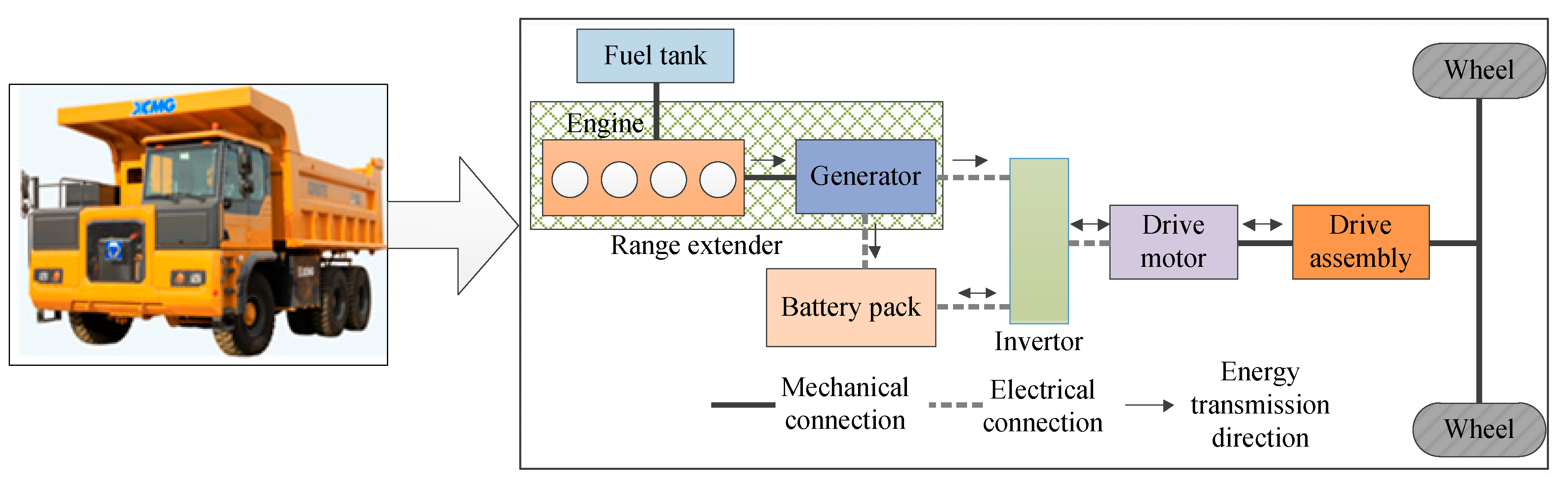
In this section, the SHE-MT is described, and its power topology is shown in Figure 1. The dynamics model of the SHE-MT and its fuel consumption optimization problem are represented, respectively. Specifically, all problems in this paper are analyzed in the discrete time domain, and the discrete time step is assumed to be 1 (s).

2.1. Dynamics Model

According to vehicle dynamics, the demand torque T wh ( t ) , speed n wh ( t ) , and power P wh ( t ) of the wheel at discrete time t can be expressed as
{ T wh ( t ) = [ m v g sin θ ( t ) + m v g cos θ ( t ) ρ f + δ m v ( t ) a ( t ) + 0.5 C D A ρ a v ( t ) 2 ] r wh n wh ( t ) = 30 v ( t ) / [ π r wh ] P wh ( t ) = T wh ( t ) n wh ( t ) / 9550
where m v , g , θ , ρ f , δ , a , C D , A , ρ a , v , and r wh denote the vehicle mass, gravity acceleration, slope angle, rolling resistance coefficient, rotational mass conversion coefficient, acceleration, air resistance coefficient, frontal area, air density, vehicle speed, and wheel radius, respectively.
The range extender consists of the engine and generator, which can provide energy to the driving motor and battery pack in the meantime. The output power of the range extender P re is equal to the electric power of the generator P g . In addition, the fuel consumption features of the range extender can be characterized by that of the engine. In other words, we can regard the engine fuel consumption rate m ˙ e as the fuel consumption rate of the range extender. The operation process and fuel consumption features of the range extender are described as (assuming the discrete time step is 1(s))
{ P re ( t ) = T re ( t ) n re ( t ) / 9550 = P g ( t ) P e ( t ) = T e ( t ) n e ( t ) / 9550 m e ( t ) = P e ( t ) m ˙ e ( T e ( t ) , n e ( t ) ) 3600 P g ( t ) = U g ( t ) I g ( t ) = T g ( t ) n g ( t ) i g ( T g ( t ) , n g ( t ) ) / 9550                 = T e ( t ) i eg n e ( t ) i g ( T g ( t ) , n g ( t ) ) / 9550 = P e ( t ) i eg i g ( T g ( t ) , n g ( t ) )                 = P e ( t ) i re ( T re ( t ) , n re ( t ) )
where T re and n re denote the torque and speed of the range extender, respectively. P e , T e , and n e represent the output mechanical power, output torque, and output speed of the engine, respectively. m e is the fuel consumption of the range extender. U g and I g represent the voltage and current of the generator, respectively. T g and n g respectively denote the input torque and speed of the generator. i eg is the mechanical transmission efficiency between the engine and generator. i g and i re are the generating efficiency of the generator and the efficiency of the range extender, respectively. The maps of m ˙ e and i re are presented in Figure 2a,b, respectively.
The battery pack can not only drive the driving motor but also recover the kinetic energy of the driving motor. The battery pack model is expressed as follows:
Δ S o C = U b + U b 2 4 P b ( t ) R b 2 C Ah R b
where U b , R b , and C Ah denote the terminal voltage, internal resistance, and capacity of the battery pack, respectively. P b represents the output electric power of the battery pack. It is further denoted as
P b ( t ) = { U b ( t ) I b ( t ) i dis ( t ) , P b ( t ) 0 U b ( t ) I b ( t ) i ch ( t ) , P b ( t ) < 0
where I b , i ch , and i dis are the loop current, charging efficiency, and discharging efficiency of the battery pack, respectively.
The driving motor can be powered by the battery pack or range extender alone or together. The operating characteristics of the driving motor are shown as
P m ( t ) = T m ( t ) n m ( t ) 9550 = { U m ( t ) I m ( t ) i m ( T m ( t ) , n m ( t ) ) , P m ( t ) 0 U m ( t ) I m ( t ) i m ( T m ( t ) , n m ( t ) ) , P m ( t ) < 0
where P m , T m , n m , U m , and I m describe the output mechanical power, output torque, output speed, voltage, and current of the driving motor, respectively. i m is the convert efficiency of driving motor between the mechanical and electric energy. The relationships among i m , T m , and n m are characterized by the map in Figure 2c. In addition, the relationships among P m , P b , and P re follow the power balance principle.
{ P m ( t ) = ( P b ( t ) + P re ( t ) ) i m ( T m ( t ) , n m ( t ) ) , P m ( t ) 0 P b ( t ) = P m ( t ) i m ( T m ( t ) , n m ( t ) ) P re ( t ) , P m ( t ) < 0
The drive assembly is able to achieve the speed reduction and torque increase of the driving motor, whose model is obtained by (1) and (5).
{ P wh ( t ) = { P m ( t ) i d , P m ( t ) 0 P m ( t ) / i d , P m ( t ) < 0 T wh ( t ) = { T m ( t ) i d i f , T m ( t ) 0 T m ( t ) i f / i d , T m ( t ) < 0 n wh ( t ) = n m ( t ) / i f
where i d and i f are the driving efficiency and speed ratio of the drive assembly, respectively.

2.2. Fuel Consumption Optimization Problem

On the basis of the established dynamics model of the SHE-MT, the fuel consumption optimization problem is described in this subsection.
According to [13], on the premise of ensuring dynamic performance, the goals of the fuel consumption optimization problem mainly include four things: (1) minimizing the equivalent fuel consumption; (2) minimizing the fuel consumption; (3) minimizing the fuel consumption and emissions; (4) minimizing the energy consumption costs. In this paper, minimizing the equivalent fuel consumption was adopted as the optimization goal of the fuel consumption optimization problem. Correspondingly, the fuel consumption optimization problem in the discrete time domain is as follows:
{ J = t = t 0 t f m ˙ f _ eqv ( t ) m ˙ f _ eqv ( t ) = m ˙ e ( T e ( t ) , n e ( t ) ) P re ( t ) i re ( T re ( t ) , n re ( t ) ) 3600 + s p P b ( t ) Q lhv
where J presents the total fuel consumption of whole trip. m ˙ f _ eqv and Q lhv indicate the equivalent fuel consumption ratio and fuel calorific value, respectively. t 0 and t f describe the start moment and end moment of the driving conditions, respectively. s is the EF and is used to convert the electricity into the equivalent fuel consumption. p denotes the penalty factor, which is related to the SoC and makes it change within the allowable range. s p is the total equivalent coefficient, and its value has a significant impact on the vehicle system performance. The determination processes of s and p are described in detail in Section 4.
Different from the torque-coupling parallel hybrid system, for the power-coupling series hybrid system, n re is not related to v . In other words, T re and n re are both changeable under the same P re . Meanwhile, when P m is determined for the SHE-MT, there are diverse power allocation approaches to distribute P m to P re and P b under the restraint (6). Different combinations of P re and P b can bring different fuel and electricity consumption rates for an identical v . For this purpose, the fuel consumption optimization goal is to determine the optimal allocation solutions of P re and P b for min ( J ) in (8).
However, for the complicated and transient working condition of the SHE-MT, the vehicle future condition information is difficult to accurately achieve in advance. Therefore, we transformed the global optimization problem in (8) into the local optimization problem to solve by adopting the MPC method. The MPC [31] method aims to obtain an optimal control strategy via minimizing the fuel consumption of the preview window. To achieve this objective, the condition information of preview window is necessary to be predicted using the MPC method first. On the basis of this, the optimal control strategy is computed on-line by means of optimal algorithms. With the vehicle driving, the predictive condition information continuously updates. Meanwhile, the optimal control sequence is obtained by rolling optimization in the prediction horizon. The specific principle is shown in Figure 3a. Correspondingly, the detailed expression is shown in (9).
min { J ( t ) = q = 0 τ 1 m ˙ f _ eqv ( t + q ) , t [ t 0 , t f τ ] } s . t . : { T e ( t ) [ T e _ min ( n e ( t ) ) , T e _ max ( n e ( t ) ) ] T re ( t ) [ T re _ min ( n r e ( t ) ) , T re _ max ( n re ( t ) ) ] n e ( t ) [ n e _ min , n e _ max ] n re ( t ) [ n re _ min , n re _ max ] S o C ( t ) [ S o C min , S o C max ] v ( t ) [ v min , v max ] P b ( t ) [ P b _ min , P b _ max ]
where τ represents the preview window size. The variable subscripts of min and max in the formula indicate the minimum and maximum values of the variables.
In this case, the MPC aims at determining the optimal control sequence u * ( t ) to min ( J ( t ) ) in each preview window, namely
u * ( t ) = arg min u ( t ) { J ( t ) = q = 0 τ 1 m ˙ f _ eqv ( t + q ) } = { u * ( t ) , , u * ( t + τ 1 ) } = { ( P re * ( t ) , P b * ( t ) ) , , ( P re * ( t + τ 1 ) , P b * ( t + τ 1 ) ) }
where u * represents the optimal power combination of the range extender and battery pack at each discrete moment. P re * and P b * denote the optimal power of the range extender and the optimal power of the battery pack at each discrete time, respectively.
Accordingly, an ECMS-MPC method is proposed to solve u * ( t ) . According to Figure 3, the vehicle speed of the SHE-MT should be known in advance to realize the ECMS-MPC on-line. A prediction model of the vehicle speed is presented to obtain the priori vehicle speed in Section 3.

3. On-Line Speed Prediction

In this section, to obtain the real-time speed trajectory, the speed prediction model needs to be established. Considering that the vehicle driving process on the actual road has strong uncertainty and nonlinearity, it is difficult for the traditional analytical model to effectively characterize the process. In other words, the speed prediction model should have the ability to adjust itself according to the road environment, that is, the parameters of the speed prediction model can be learned and updated [42]. With the help of its information inheritance and real-time prediction advantages, an RNN [36,37,38] can not only have an excellent fitting effect on the nonlinear mapping relationship between the input and output of uncertain systems, but it also can learn by itself by means of data. Therefore, an RNN is applied to build the speed prediction model in this subsection. Specifically, for improving the predictive precision of the RNN, with the help of an off-line database, we utilize the hybrid optimization method of the PSOA-GA to optimize the initial parameters of the prediction model. On this basis, the framework and implementation process of on-line speed prediction based on an RNN are described in detail.

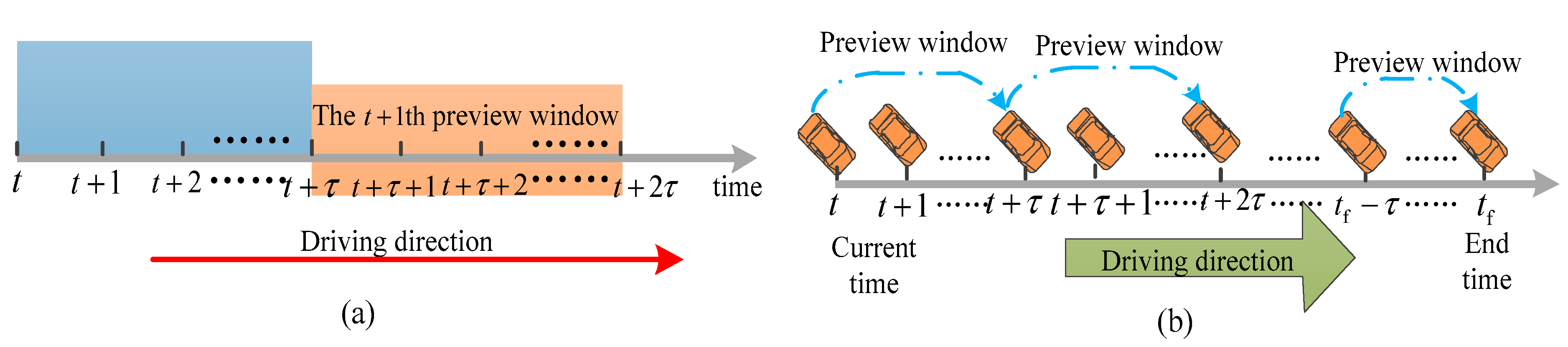
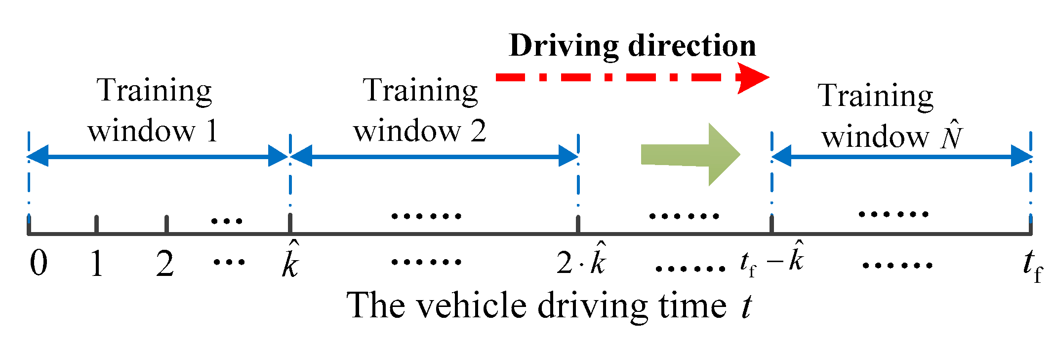
3.1. Vehicle Speed Prediction Problem

First, the prediction principle of the vehicle speed is analyzed. In general, the speed prediction uses the history states information to predict the future speed information in limited space or time, and its process is described in Figure 3b. According to vehicle theory, the kinematic equation of a vehicle under ideal conditions is described as (assuming the discrete time step is 1(s))
v ( t + 1 ) = v ( t ) + a ( t )
However, in practical conditions, the variation of the vehicle speed, not only relating to its motion state but also affected by the driver habits and road slope, is a highly nonlinear change process. Considering that the driver’s driving habits are strongly related to a ( t ) , we use a ( t ) to characterize the driver’s habits. In addition, it can be seen from (1) that slope angle θ ( t ) can directly affect the longitudinal motion state of the vehicle. For this reason, the state space equation of the vehicle speed in practical conditions can be denoted as
v ( t + 1 ) = ξ ( v ( t ) , a ( t ) , θ ( t ) , t )
where ξ denotes the v ( t ) to v ( t + 1 ) evolution model. Obviously, the key to solving the speed prediction problem is to determine the ξ specific form in (12). Considering the continuity and nonlinearity of speed variation, an RNN [36,37,38] has inherent advantages in solving this problem. Thus, the speed prediction model is established based on RNN in the next subsection.

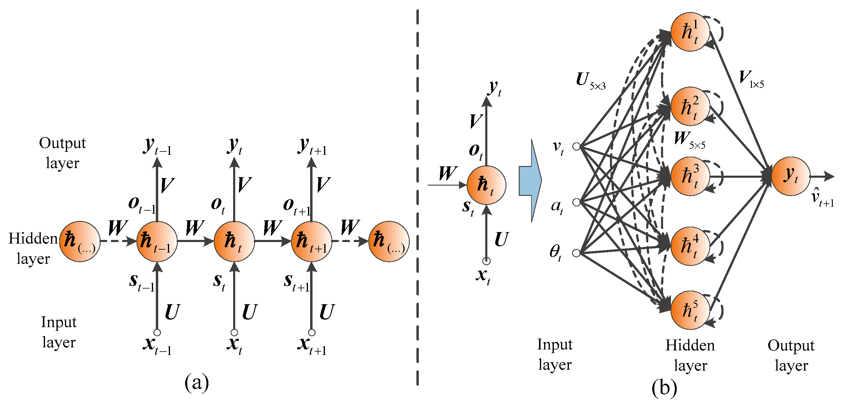
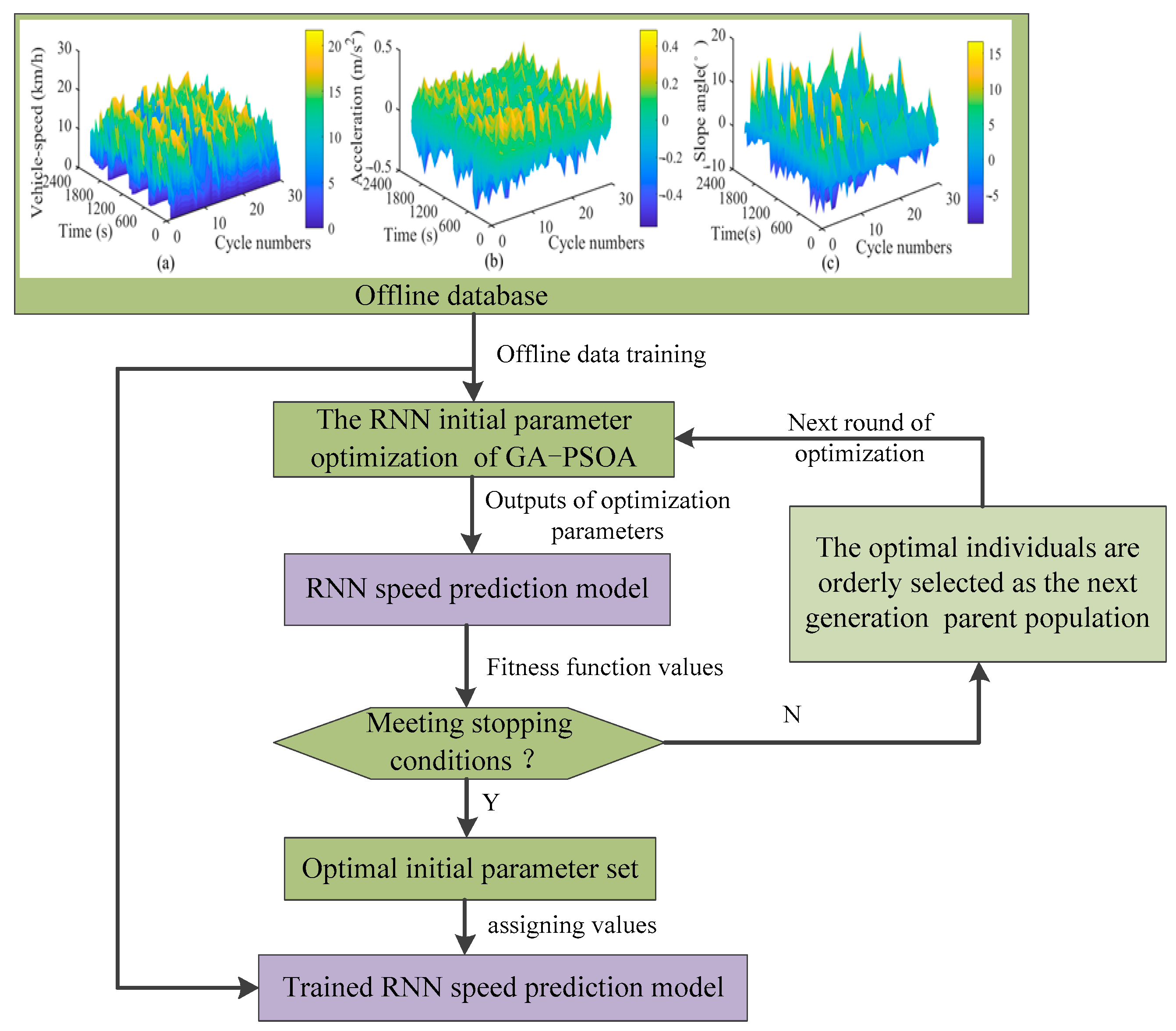
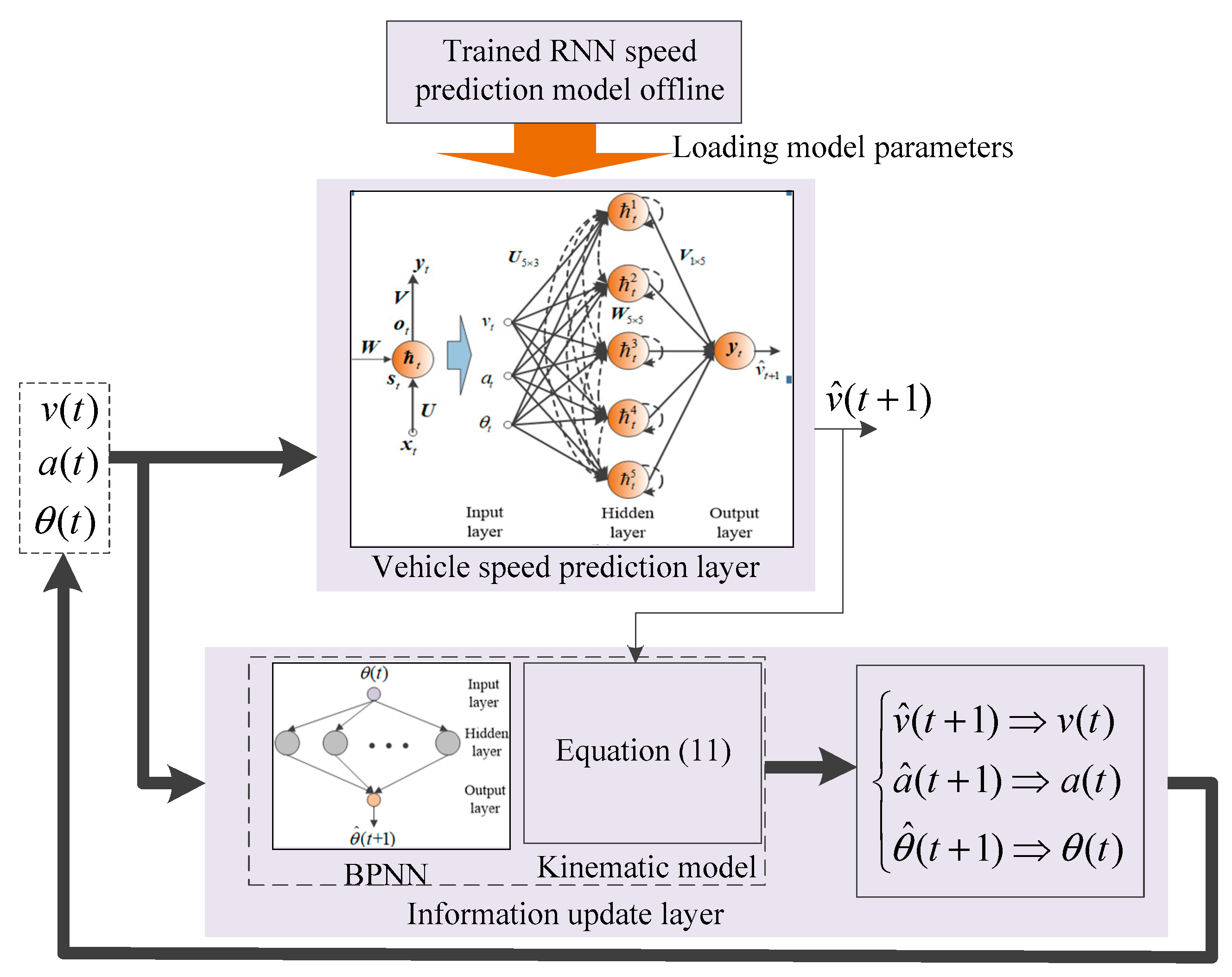
3.2. Speed Prediction Model Based on RNN

An RNN [36] is a special artificial neural network that is usually used to solve time series problems [43]. It is composed of a series of neurons with the same structure. The neurons of an RNN have a memory state. When processing sequence data, the input not only contains sequence data but also the memory state of the previous moment [44]. The general structure of an RNN is shown in Figure 4a, whose networks include the input layer, hidden layer, and output layer. In the discrete time series k ^ , the information transmission relation of the nodes in each layer network at discrete time t can be expressed as
{ s t = U × x t + W × t 1 t = g ( s t ) o t = V × t y t = σ ( o t )
where x t and y t indicate the input and output vectors of the RNN, respectively. s t and t describe the input and output vectors of the hidden-layer nodes, respectively. o t is the input vector of the output-layer nodes. g and σ represent the activation functions of the hidden-layer nodes and output-layer nodes [38], here selecting the tanh and purelin functions, respectively. U , W , and V express the weight matrixes of the input-layer nodes to the hidden-layer nodes, the hidden-layer nodes to the hidden-layer nodes, and the hidden-layer nodes to the output-layer nodes, respectively.
According to (13), t not only relates to x t but also to t 1 . In other words, the network outputs at discrete time t inherit the network state information at discrete time t 1 . The inheritance relationship has inherent advantages for representing the speed prediction model via the time series evolution in (12). Hence, a speed prediction model is established using an RNN, which takes the speed, acceleration, and slope angle as the inputs and the prediction speed as the output. The node numbers of the input layer, hidden layer, and output layer satisfy the following empirical expression [38]:
m = i + n + λ , λ [ 1 , 2 , , 10 ]
where i , m , and n denote the node numbers of the input layer, hidden layer, and output layer, respectively. In this paper, the RNN structure of the speed prediction model is 3-5-1, as described in Figure 4b.
Then, the speed prediction process of the model is analyzed. It can be seen in Figure 4b that the specific expression form of the speed prediction model at discrete time t is as follows:
{ s t = U 5 × 3 × [ v t , a t , θ t ] T + W 5 × 5 × t 1 t = tanh ( s t ) o t = V 1 × 5 × t v ^ t + 1 = o t
where v t , a t , and θ t show the speed, acceleration, and slope angle at discrete time t , respectively. v ^ t + 1 represents the prediction speed at discrete time t + 1 . The specific forms of U , W , V and t can be further described as
U : U 5 × 3 = [ U 11 U 12 U 13 U 21 U 22 U 23 U 31 U 32 U 33 U 41 U 42 U 43 U 51 U 52 U 53 ]
W : W 5 × 5 = [ W 11 W 15 W 51 W 55 ] T
V : V 1 × 5 = [ V 11 V 12 V 13 V 14 V 15 ]
t : t = [ t 1 t 2 t 3 t 4 t 5 ] T
Obviously, once t , U , W , and V at t = 0 are determined, we can utilize (15) to predict the speed on-line. In addition, in order to ensure the speed prediction accuracy of the model, U , W , and V are continually learned through the supervised learning method until the model prediction error L satisfies the set target value:
L = j = 1 k ^ ( 1 2 v ^ t + j v t + j 2 ) ε
where ε 0 is a target error.
Next, we continue to analyze the parameter learning process. The gradient descent method was adopted to update U , W and V . The variation of V can be expressed as
Δ V 1 × 5 = η L V 1 × 5 = η j = 1 k ^ ( v ^ t + j v t + j ) t + j T
where η ( 0 , 1 ] is the learning factor.
As known from (15), the variation of W can influence the outputs of the hidden-layer nodes at the current and next moments. Therefore, the variation of t is defined as
δ t + j = L t + j = L o t + j ( o t + j t + j ) T + L t + j + 1 ( t + j + 1 t + j ) T                     = { ( v ^ t + j v t + j ) V 1 × 5 T + [ W 5 × 5 T × d i a g ( 1 ( t + j + 1 ) 2 ) ] × δ t + j + 1 , j < k ^ ( v ^ t + j v t + j ) V 1 × 5 T , j = k ^
Further, the variation of W can be obtained as
Δ W 5 × 5 = η L W 5 × 5 = η j = 1 k ^ ( L t + j t + j W 5 × 5 )   = η j = 1 k ^ ( d i a g ( 1 ( t + j ) 2 ) × δ t + j × t + j 1 T )
The variation of U can be obtained by means of the analysis scheme of W .
Δ U 5 × 3 = η L U 5 × 3 = η j = 1 k ^ ( L t + j t + j U 5 × 3 )                                           = η j = 1 k ^ ( d i a g ( 1 ( t + j ) 2 ) × δ t + j × x t + j T )
Therefore, U , W , and V can be updated using the following equation:
{ U 5 × 3 t + k ^ = U 5 × 3 t + Δ U 5 × 3 W 5 × 5 t + k ^ = W 5 × 5 t + Δ W 5 × 5 V 1 × 5 t + k ^ = V 1 × 5 t + Δ V 1 × 5
Based on the above analysis, to complete the speed prediction and parameter training of the prediction model, 0 , U , W and V of the RNN are required to be initially assigned. However, in this process, different initial values can directly affect the training effect and prediction accuracy of the RNN. Accordingly, to further improve the model prediction accuracy, the hybrid optimization method of the GA-PSOA proposed in our previous work [14] is selected to determine the optimally initial parameters of the RNN. The specific algorithm details refer to the previous work in [14], not mentioned here. The training process of the RNN speed prediction method based on the GA-PSOA is expressed in Figure 5. Correspondingly, its implementation procedures are indicated as follows.
Step 1: The parameters of U , W , V and 0 need to be sequentially encoded, producing individuals and populations. By means of (17) in [14], S individuals and populations consisting of S individuals of the GA and PSOA are initialized, respectively. Namely, the GA and PSOA have populations consisting of S individuals, respectively.
Step 2: Equation (20) is taken as the fitness function to calculate the fitness value of each individual.
Step 3: Each individual of the two populations assigns its own parameters to U , W , V , and 0 . In the meantime, the fitness values of the 2 S individuals are calculated by (15) and (20). By comparing the individual fitness values of the GA and PSOA sequentially, the S individuals whose fitness values are the smaller are chosen from the 2 S individuals as the collective parent population of the GA and PSOA.
Step 4: According to the collective parent population, the GA and PSOA generate their own child populations by means of their respective population-updating mechanisms.
Step 5: The fitness values of the 2 S child individuals of the two child populations are calculated by (15) and (20). By comparing the individual fitness values of the two child populations sequentially, we select the S individuals with smaller fitness values from the 2 S child individuals, forming a new child population. By comparing the individual fitness values of the new child population and collective parent population sequentially, the S individuals with smaller fitness values are selected from the 2 S individuals as the new population for the next iteration of the GA and PSOA.
Step 6: The optimal individual of the new population in Step 5 is selected as the new parent individual for next iteration of the GA and PSOA.
Step 7: Judge whether the iteration reaches the set value or L meets (20). If it satisfies these conditions, the new parent individual in Step 6 is taken as the optimal initial parameters of the RNN, and its values are sequentially assigned to U , W , V , and 0 in (15), going to Step 8. Otherwise, taking the new population obtained in Step 5 as the collective parent population, the algorithm goes back to Step 4.
Step 8: The RNN uses the offline database to continuously train (15) and updates U , W and V using (21)–(25) until L meets (20).
On the basis of the above-established model, we can predict the speed. However, for achieving speed prediction on-line, the acceleration a ^ and slope angle θ ^ in the prediction window need to be obtained in advance. Here, a ^ can be determined based on (11) when the vehicle speeds at adjacent times are known. A backpropagation neural network (BPNN) [45] is employed to build the prediction model of θ ^ , and the prediction principle and execution process of the BPNN is referred to in our previous work [14], so the details are not shared here. An offline database is used to train the BPNN. Based on the above work, the framework of speed prediction on-line is established in Figure 6. The vehicle speed prediction layer predicts speed on-line by using the trained RNN model. The information update layer updates v ^ , a ^ and θ ^ . Its specific implementation process is as follows.
Step 1: τ is determined.
Step 2: The vehicle speed prediction layer uses v ( t ) , a ( t ) , and θ ( t ) to predict v ^ ( t + 1 ) .
Step 3: The information update layer utilizes a ( t ) and θ ( t ) to predict a ^ ( t + 1 ) and θ ^ ( t + 1 ) , and updates the input information of the vehicle speed prediction layer in the next moment.
Step 4: If t < τ , then go back to Step 2. Otherwise, go back to Step 1 until the trip is over.
In addition, as the vehicle continues to drive, new driving cycle data are continuously generated. To ensure the adaptability of the model to the random working conditions of the mine truck, the speed prediction model is updated using data obtained on-line, taking the k ^ of the RNN as the training window size, that is, the model is only trained at k ^ l time, l { 1 , 2 , , N ^ } , as shown in Figure 7. By means of the process, the model parameters in Figure 6 are continuously updated. With the help of the obtained speed trajectory, the ECMS-MPC can achieve the on-line optimization of fuel consumption, the detailed description of which is shown in the next section.

4. ECMS Based on Model Predictive Control
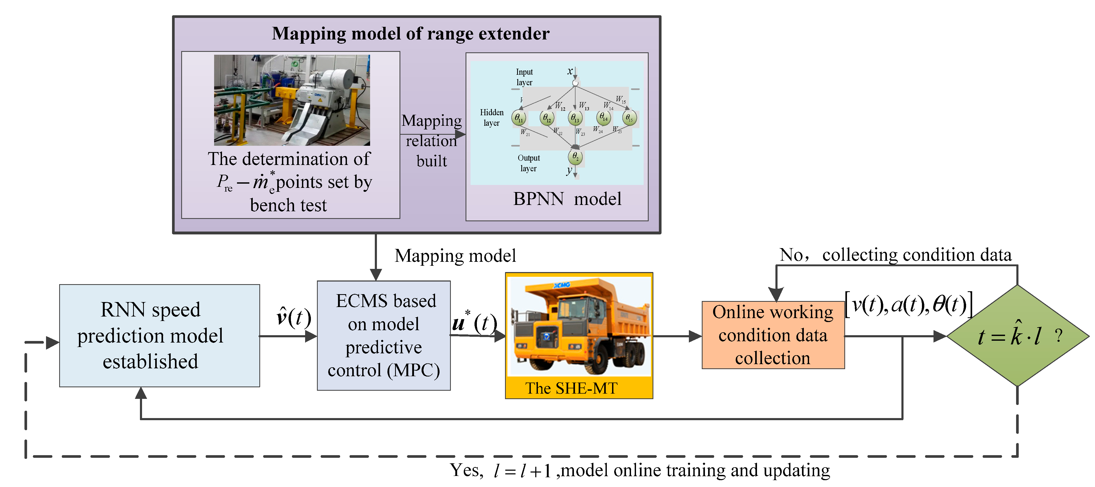
Based on the above analysis, while the vehicle velocity of the preview window is obtained on-line, it is very necessary for MPC to select a rational optimization algorithm to calculate (10) on-line. This paper fully integrates the ECMS instantaneous optimization advantage and MPC optimization idea, designing a novel ECMS based on MPC. In this process, for improving the calculation speed and real-time performance of the proposed EMS, the power-optimal fuel consumption mapping model of the range extender is established. In addition, to further improve the adaptability to random conditions of the SHE-MT, the EF is dynamically adjusted using the PSOA.

4.1. P re m ˙ e * Mapping Model

According to the range extender model in Section 2, the relationship between the power and fuel consumption of the range extender is a highly nonlinear system. For the same P re , there exist various combinations of T re and n re , producing different fuel consumption rates. Therefore, the power P re —optimal fuel consumption m ˙ e * ( P re m ˙ e * ) mapping model of the range extender needs to be determined in advance. The specific steps of the implementation process are as follows.
First, we need to find the optimal fuel consumption point for each power point of the range extender, obtaining the P re m ˙ e * points set. This is usually determined through two methods at present. One is based on the range extender map data using the (2) and (26) traversal search; the other is based on a bench test, which is directly measured.
{ P re = T e n e 9550 i re ( T re , n re ) m ˙ e * = min ( m ˙ e ( T e , n e ) )
Here, we adopted the bench test to obtain the P re m ˙ e * points set. Then, considering the highly nonlinear relationship between P re and m ˙ e * , the BPNN [45] was used to establish the P re m ˙ e * mapping model. According to (14), the BPNN with a 1-5-1 structure was selected. The specific training process of the BPNN was also described in our former research [14], so the details are not shared here. Based on the above analysis, the P re m ˙ e * mapping model of the range extender was determined.

4.2. The Realization Process of ECMS-MPC

Combining the speed trajectory obtained on-line and the established P re m ˙ e * mapping model, the realization framework of the proposed ECMS-MPC is described in Figure 8, whose specific implementation process is as follows, assuming that the current time is the t th (s).
Step 1: Based on v ( t ) , a ( t ) , and θ ( t ) , the RNN speed prediction model outputs the speed sequence v ^ ( t ) = { v ^ ( t + 1 ) , , v ^ ( t + τ ) } in the future τ .
Step 2: The demand power sequence of the driving motor P m = { P m ( t + 1 ) , , P m ( t + τ ) } in τ is calculated using v ^ ( t ) , (1), and (7).
Step 3: Based on P m and the obtained P re m ˙ e * mapping model, the optimal EF set s * in the current τ is solved using the PSOA. The detailed process of the s * solution is shown in Algorithm 1. p is given by:
p = 1 S o C S o C t arg et S o C max S o C min
where S o C t arg et , S o C max , and S o C min are the target, maximum, and minimum values of the SoC, respectively. Here, we set S o C min as S o C t arg et .
Step 4: According to the obtained s * and p in Step 3, the optimal output power combination sequence u * ( t ) = { ( P re * ( t ) , P b * ( t ) ) , , ( P re * ( t + τ 1 ) , P b * ( t + τ 1 ) ) } of the range extender and battery pack is calculated using (8) and (9), and sends u * ( t ) to the vehicle.
Step 5: After the SHE-MT runs forward by executing u * ( t ) , v , a , and θ will be instantly updated. When t = t + τ (s), the ECMS-MPC goes back to Step 1 and enters the next round of MPC regulation. In this process, the vehicle will always collect the condition information on-line, and the speed prediction model can be trained real-time and updated at k ^ l time.
Based on the above analysis, with the vehicle driving continually, the above-mentioned control process can be continuously conducted in a rolling way until the SHE-MT reaches its destination.
Algorithm 1: The s * solution on the basis of PSOA.
// Step 1: The initialization of parameters:
ϑ , c 1 , c 2 , ψ , r 1 and r 2 of (22) in [14]; G max , S in [14], τ ;
// Step 2: Fitness function determination:
Executing (9);              // Initializing fitness function
// Step 3: Initializing individual and population:
G = 1;                     // Generating  G th population
for  ζ = 1, ζ < = S , ζ + +       // Generating individual of PSOA
    Conducting (17) in [14];  // Encoding individual
    Conducting (9);  // Calculating fitness value
end for
I G Conducting (17) in [14];  // Generating the G th population as the parent population of PSOA
J PSOA Fitness values of S individuals;
// Step 4: Reforming child population on the basis of PSOA:
I Child I G ;    //  PSOA’s population regeneration
for   ζ = 1, ζ < = S , ζ + + // Reforming child population for PSOA
    Conducting  (22) in [14];         // Updating individual
    Conducting  (9);         // Calculating Fitness
end for
I Child Conducting (17) in [14];
J child Fitness values of S individuals;
// Step 5: Generating new parent population of PSOA:
G G + 1 ;     // Updating G
I G Selecting the individuals with smaller fitness values sequentially to form a population from { I G 1 , I Child } ;      
// Forming the new parent population
// Step 6: Judging stopping conditions:
I opt Choosing the optimal individual in I G ;
if  G > = G max        // Satisfying stopping conditions
    Going back I opt ;               // Outputting I opt
    Producing Step 7;                     
else
    Returning to Step 4;   // Forming new population
end if
// Step 7: Taking I opt as s * .

5. Results and Discussion

A cement mine road was adopted as the research route, as shown in Figure 9. First, to verify the speed prediction effect of the RNN, the speed prediction model was simulated and analyzed carefully, including the initial parameter determination of the RNN model, prediction and training window selection, and speed prediction effect. Then, the performances of the DRB EMS, FRB EMS, ECMS, and the proposed ECMS-MPC are compared and discussed in detail.

5.1. Experimental Setup

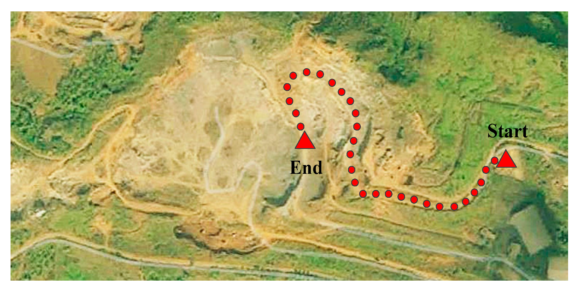
5.1.1. Cycle Selection

As shown in Figure 9, the distance of the cement mine road was 7.9 km. Correspondingly, the speed, acceleration, and slope angle information of 30 cycles of a SHE-MT were collected, as shown in Figure 10.

5.1.2. Model Training Parameters

In order to ensure the training effect, the training and test samples accounted for 70% and 30%, respectively. Meanwhile, for ensuring the learning speed and accuracy of the model, we took η = 0.1 and ε = 0.0001, respectively. In addition, to eliminate calculation deviation, we normalized the samples according to the following formula.
r = ( R R min ) / ( R max R min )
where R , R min and R max represent the real value and lower and upper limits of the samples, respectively. r denotes the normalized value of R , R [ R min , R max ] .

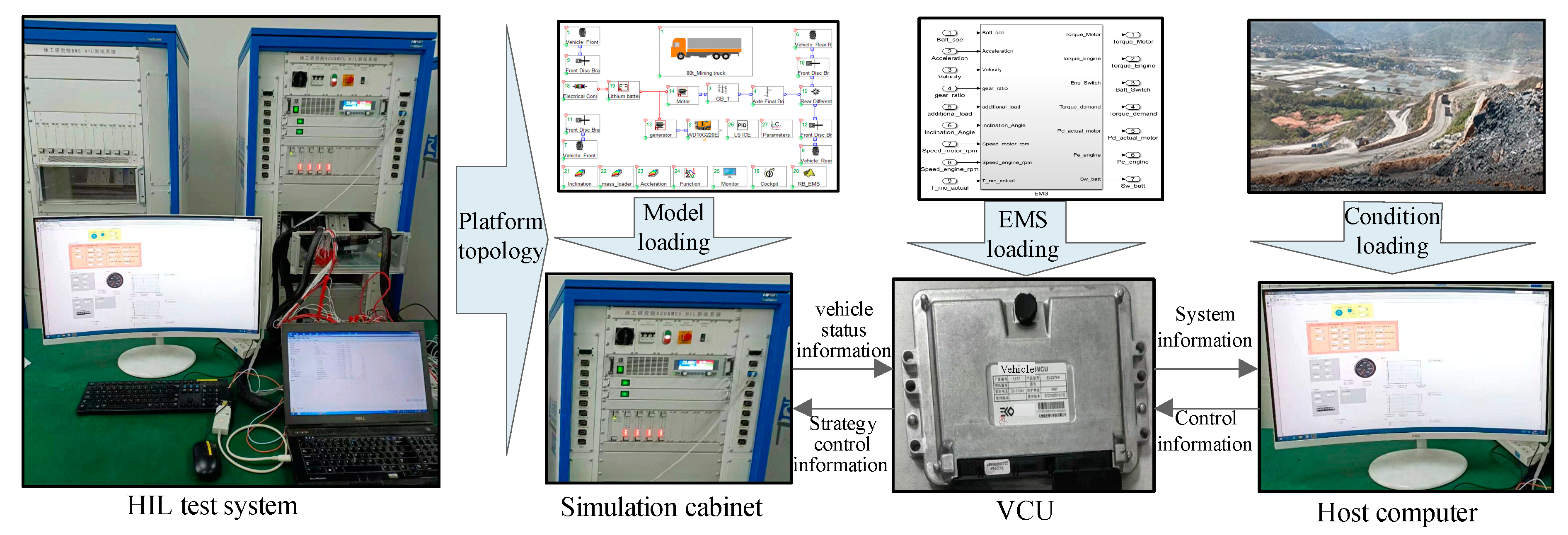
5.1.3. Simulation Platform Establishment

In order to fully verify the effectiveness and real-time performance of the proposed EMS, the experimental simulation platform was established by using a hardware-in-loop (HIL) bench, as shown in Figure 11. The vehicle parameters of the SHE-MT are indicated in Table 1.

5.1.4. Error Evaluation Methods

The prediction results were evaluated by four errors, namely the absolute error A E , the mean absolute error M A E , the root mean square error R M S E , and the mean relative error M R E . The detailed expressions of the four errors are illustrated by (26) in [14].

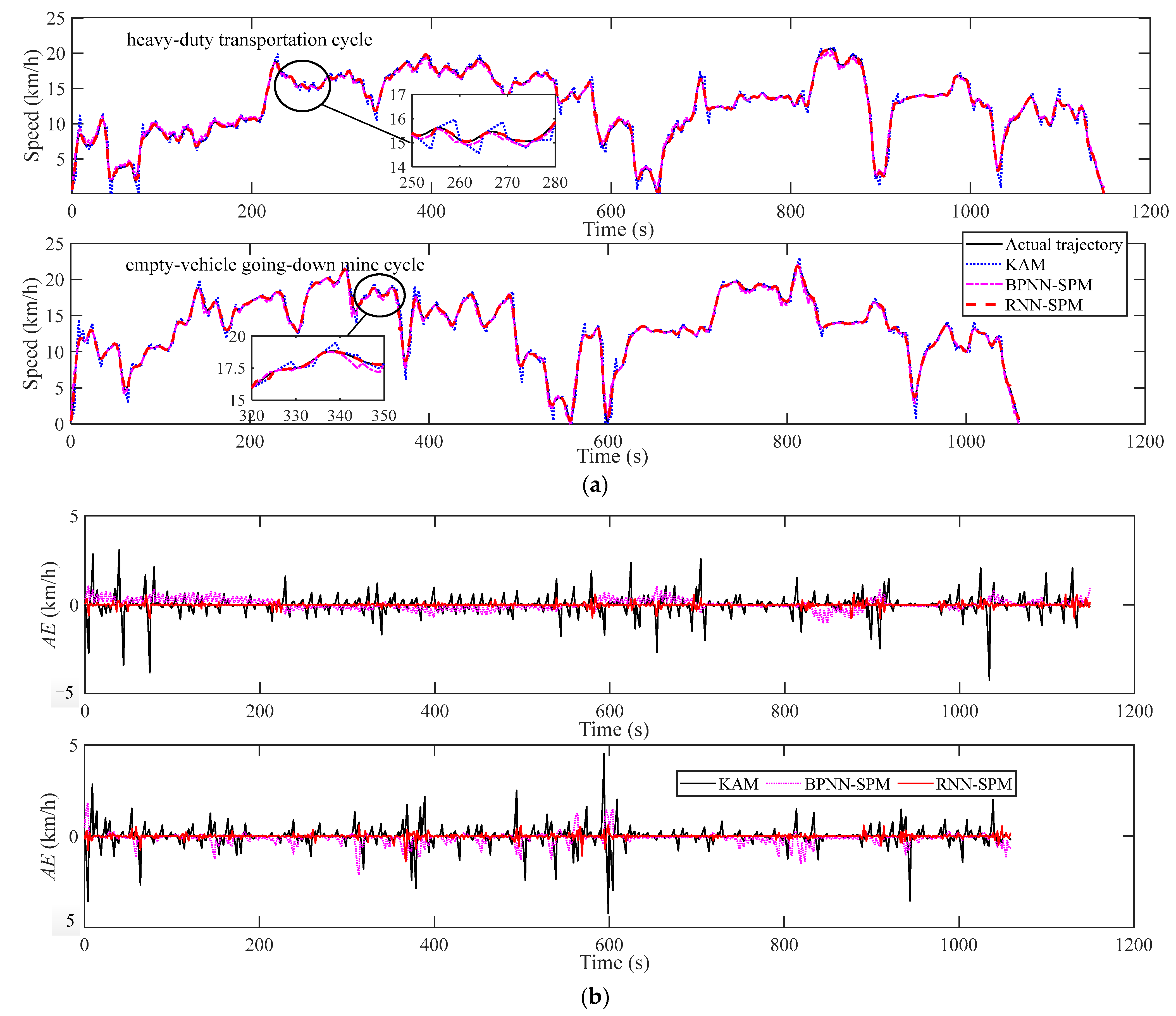
5.2. Analysis of the Speed Prediction

5.2.1. The Initial Parameter Setting

As described above, different initial values can directly affect the training effect and prediction accuracy of the RNN. To verify the optimal effect of the hybrid optimization method, the GA, PSOA, and hybrid optimization method based on the GA-PSOA were used to find the optimal initial parameters of U , W , V , and 0 , respectively.
It can be seen from (20) that the individual’s fitness value can characterize the merits and demerits of its initial parameters. In general, the algorithm optimization effect can be evaluated by the average fitness value of the population. In other words, the algorithm optimization effect is better when the population’s average fitness value is smaller. According to the collected vehicle condition information described in Figure 10, we achieve the changing relationships of the average fitness values of the three algorithms with iterations, as described in Figure 12. The convergence speed of the average fitness value of the hybrid optimization algorithm is faster than that of the GA and PSOA under the same optimization conditions. Furthermore, while satisfying the stopping conditions, its average fitness value is smaller than that of the other two algorithms. Correspondingly, the optimal initial network parameters of the RNN are shown in Table 2.

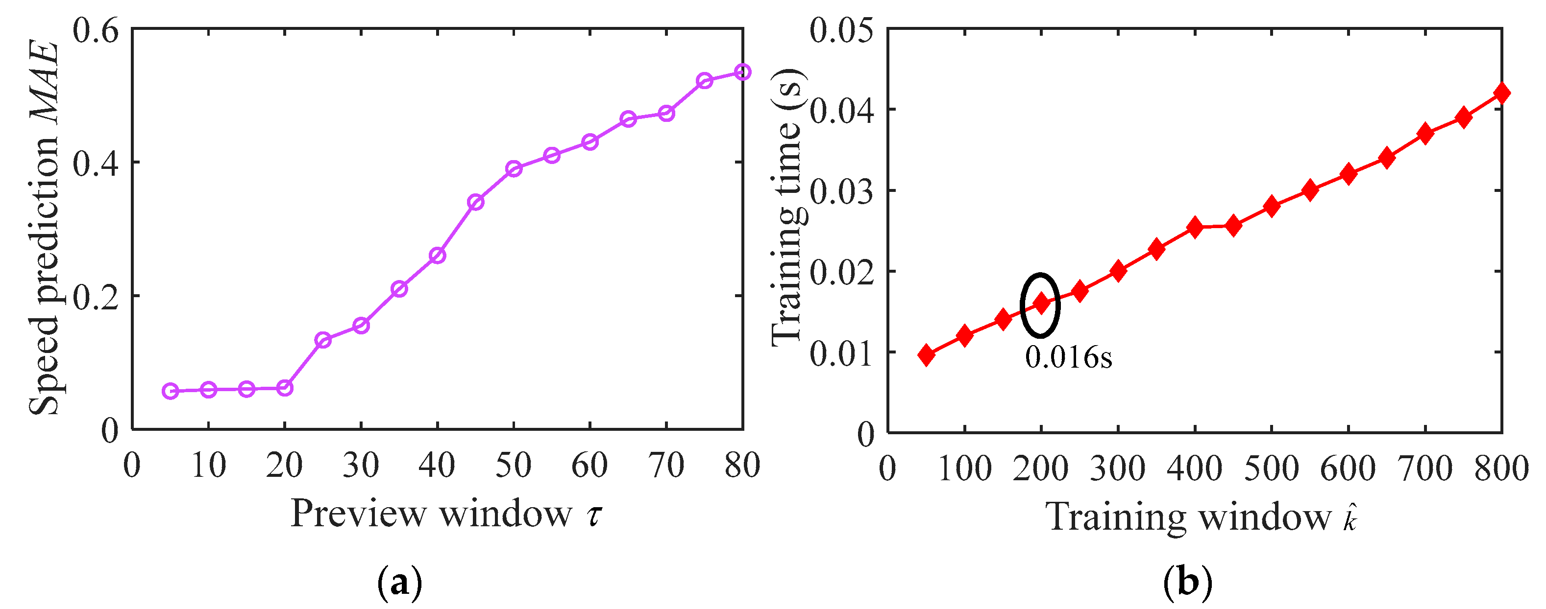
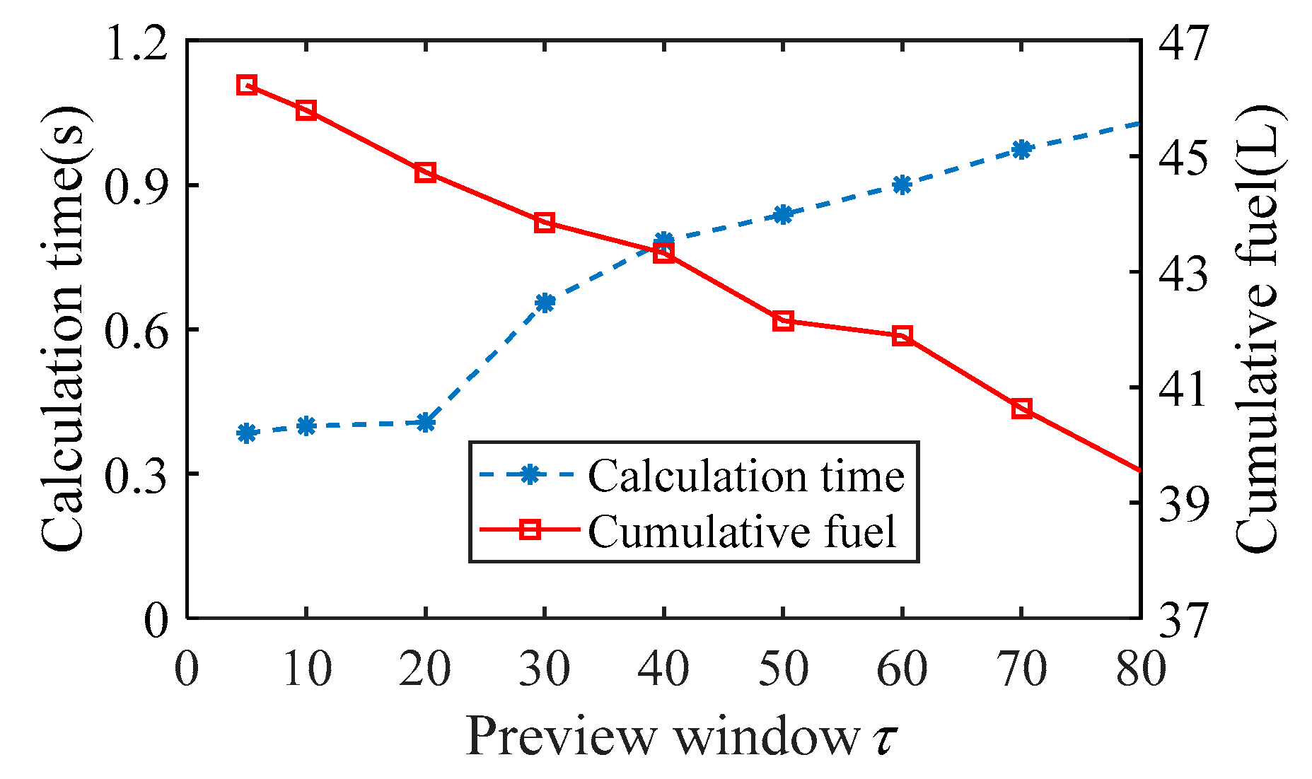
5.2.2. Selection of τ and k ^

First of all, as shown in Figure 3, τ characterizes the preview window size, which can influence the prediction accuracy of the speed. Therefore, it is very essential to select the appropriate τ to ensure the accuracy of the predicted speed trajectory. The relationship of the speed prediction MAE with τ is shown in Figure 13a. Considering the speed prediction effect, we set τ = 20.
Secondly, based on Section 3, k ^ not only characterizes the time series of the RNN but is also used to characterize the size of the training window. For this purpose, to ensure the real-time performance of the prediction and parameter training, selecting a rational k ^ is also significant. The relationship of the training time with k ^ is displayed in Figure 13b. Considering that the single running time of the vehicle control unit (VCU) on the actual vehicle is 20 ms, to complete the training process in 20 ms, k ^ was set to 200.

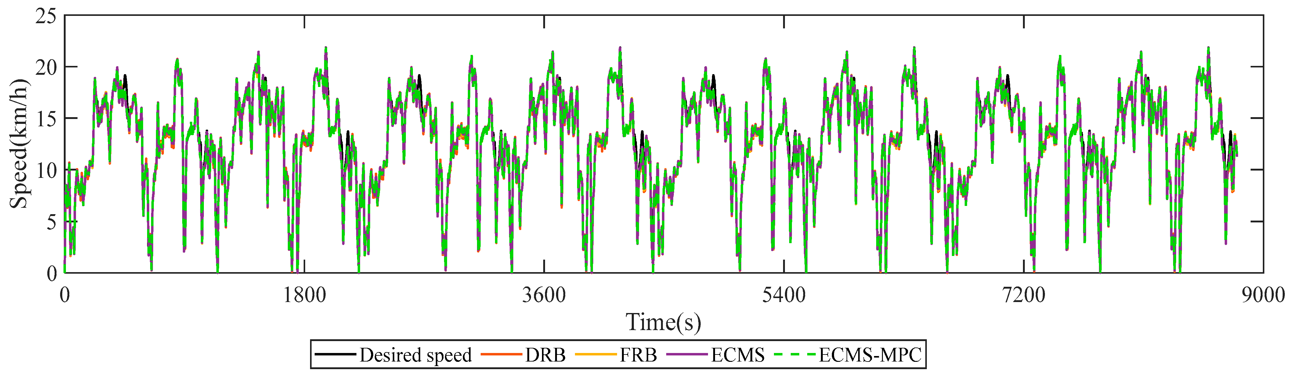
5.2.3. Speed Prediction Analysis

For covering the generality of the working conditions, the heavy-duty transportation cycle and empty-vehicle going-down-mine cycle were selected as the experimental simulation conditions. On this basis, the kinematics analysis method (KAM), the BPNN speed prediction method (BPNN-SPM), and the RNN speed prediction method based on the GA-PSOA (RNN-SPM) were utilized to predict the speed. Accordingly, the relationships and AE between the predictive and actual speed trajectories of the three methods are represented in Figure 14. Table 3 gives the MAE, RMSE and MRE of the three methods.
First, according to Figure 14a, the changing trends of the speed prediction trajectories obtained by the three methods followed the changing trend of the actual speed, but their corresponding ranges of A E were different. Specifically, the A E ranges of the KAM, BPNN-SPM, and RNN-SPM under the two conditions were [−4.259 km/h, 3.078 km/h] and [−4.246 km/h, 4.522 km/h], [−1.043 km/h, 1.089 km/h] and [−2.127 km/h, 1.838 km/h], and [−0.755 km/h, 0.589 km/h] and [−1.388 km/h, 0.617 km/h], respectively. It is thus clear that the A E changing range of the RNN-SPM was less than that of the other two methods.
Secondly, as shown in Table 3, the M A E , R M S E and M R E of the proposed RNN-SPM ere the smallest among the three methods. Specifically, in comparison to the KAM and BPNN-SPM, the M A E , R M S E and M R E of the RNN-SPM respectively decreased by 77.0%, 73.2%, and 75.1% and 72.0%, 51.8%, and 69.9% under the heavy-duty transportation cycle. Compared to the KAM and BPNN-SPM, under the empty-vehicle going-down-mine cycle, the M A E , R M S E and M R E of the RNN-SPM were reduced by 76.7%, 73.1%, and 78.1% and 69.3%, 58.3%, and 70.1%, respectively. In addition, the speed prediction accuracies of the RNN-SPM under the two working cycles both exceeded 98% (namely, speed prediction precision = 1 M R E ).
Based on the above analysis, on the premise of assuring real-time performance, the designed RNN-SPM effectively improved the speed prediction accuracy and better adapted to the stochastic conditions of the SHE-MT.

5.3. Performance Analysis of EMS

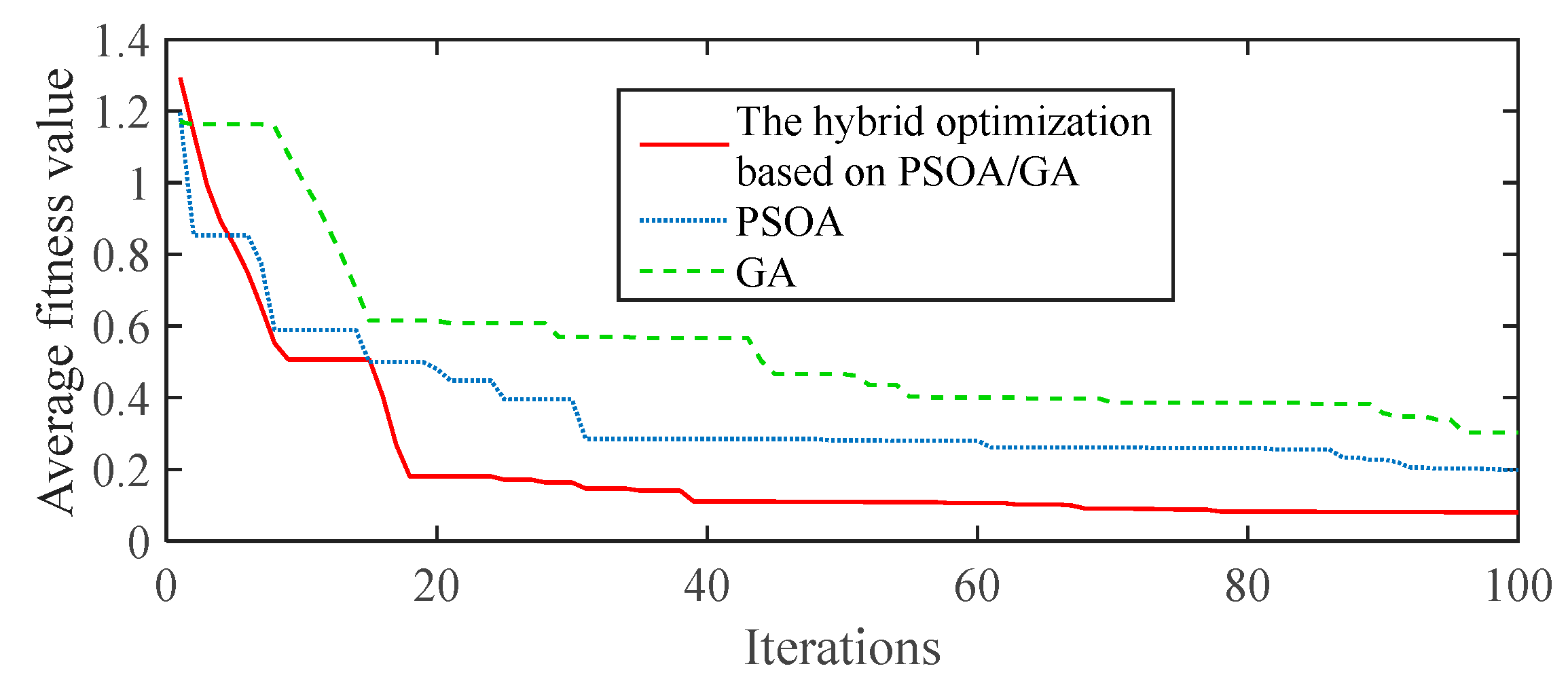
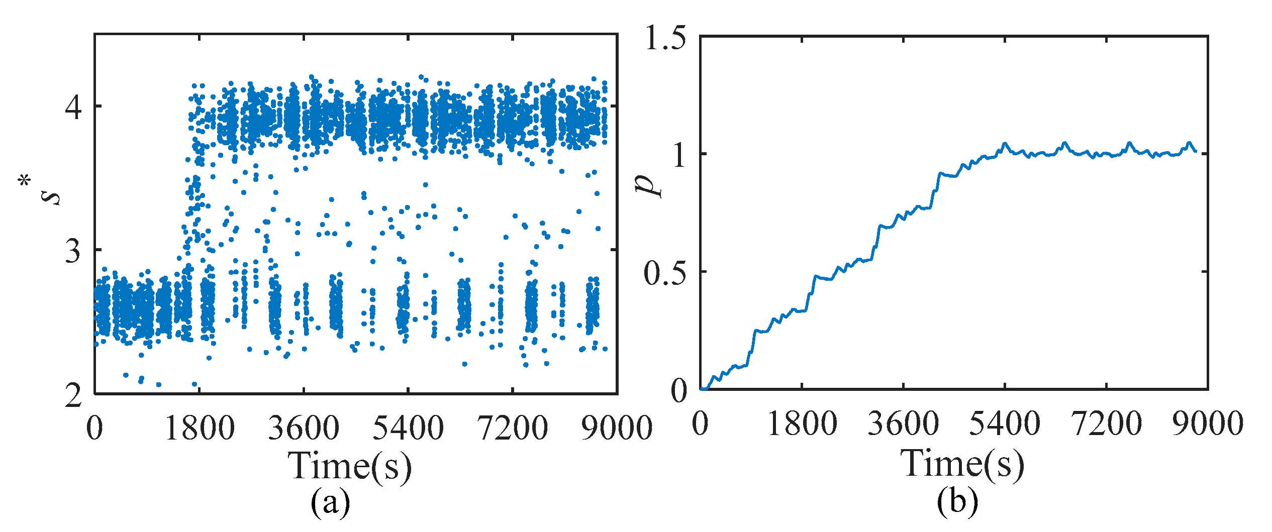
5.3.1. Parameter Determination of the ECMS-MPC

In the analysis part of the speed prediction model, τ was preliminarily selected to ensure the accuracy of the speed prediction. Nevertheless, the fuel consumption and calculation time of the ECMS-MPC are also related to τ . For this reason, the relationships between the calculation time and the fuel consumption of the ECMS-MPC with τ are described in Figure 15. Based on Figure 13a and Figure 15, with the increase in τ , although the fuel consumption optimization effect of the proposed EMS became better, its real-time performance and speed prediction accuracy became worse. Therefore, comprehensively considering the speed prediction accuracy, real-time performance, and fuel consumption optimization effect, τ was still set to 20 in this paper.

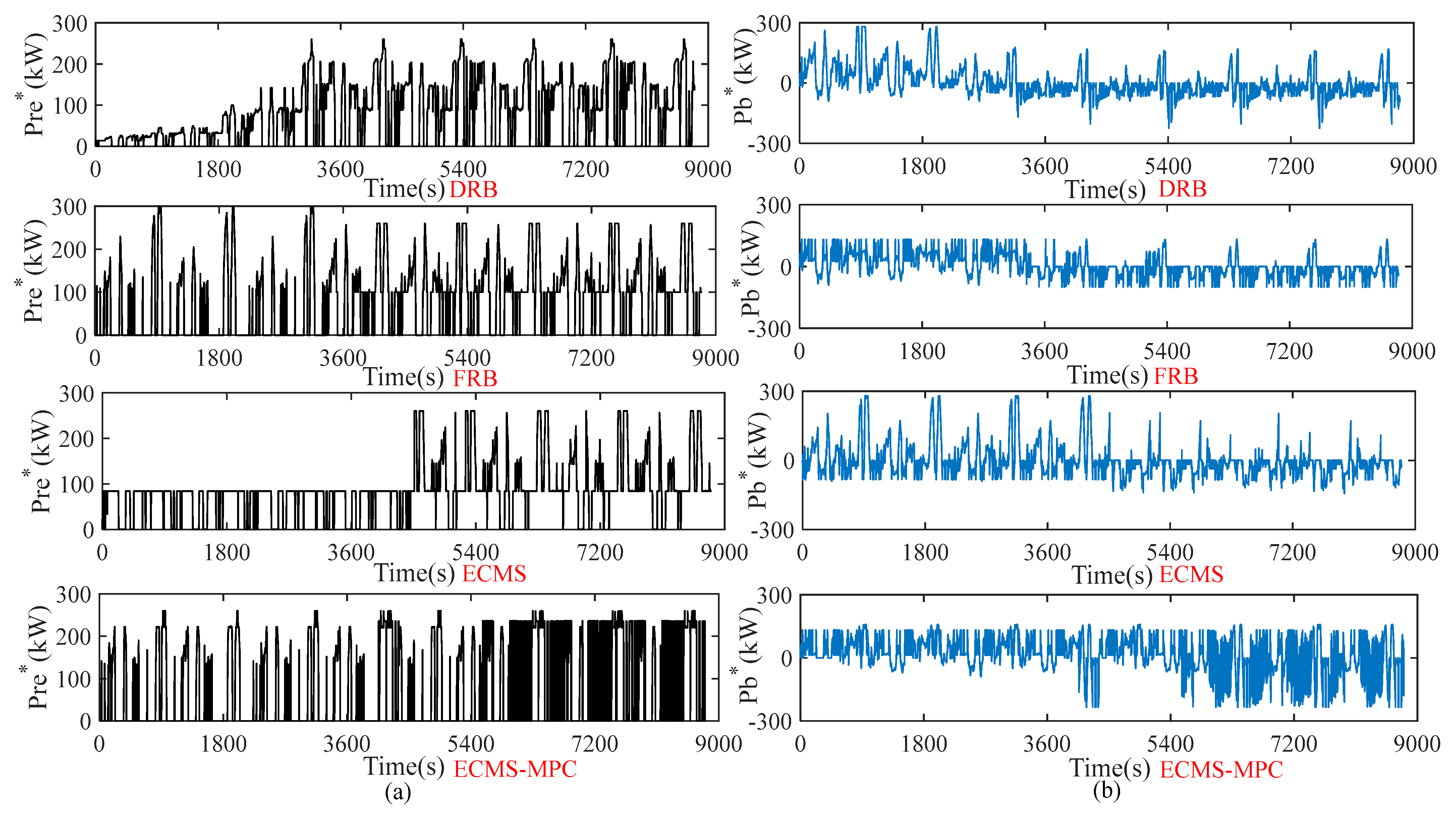
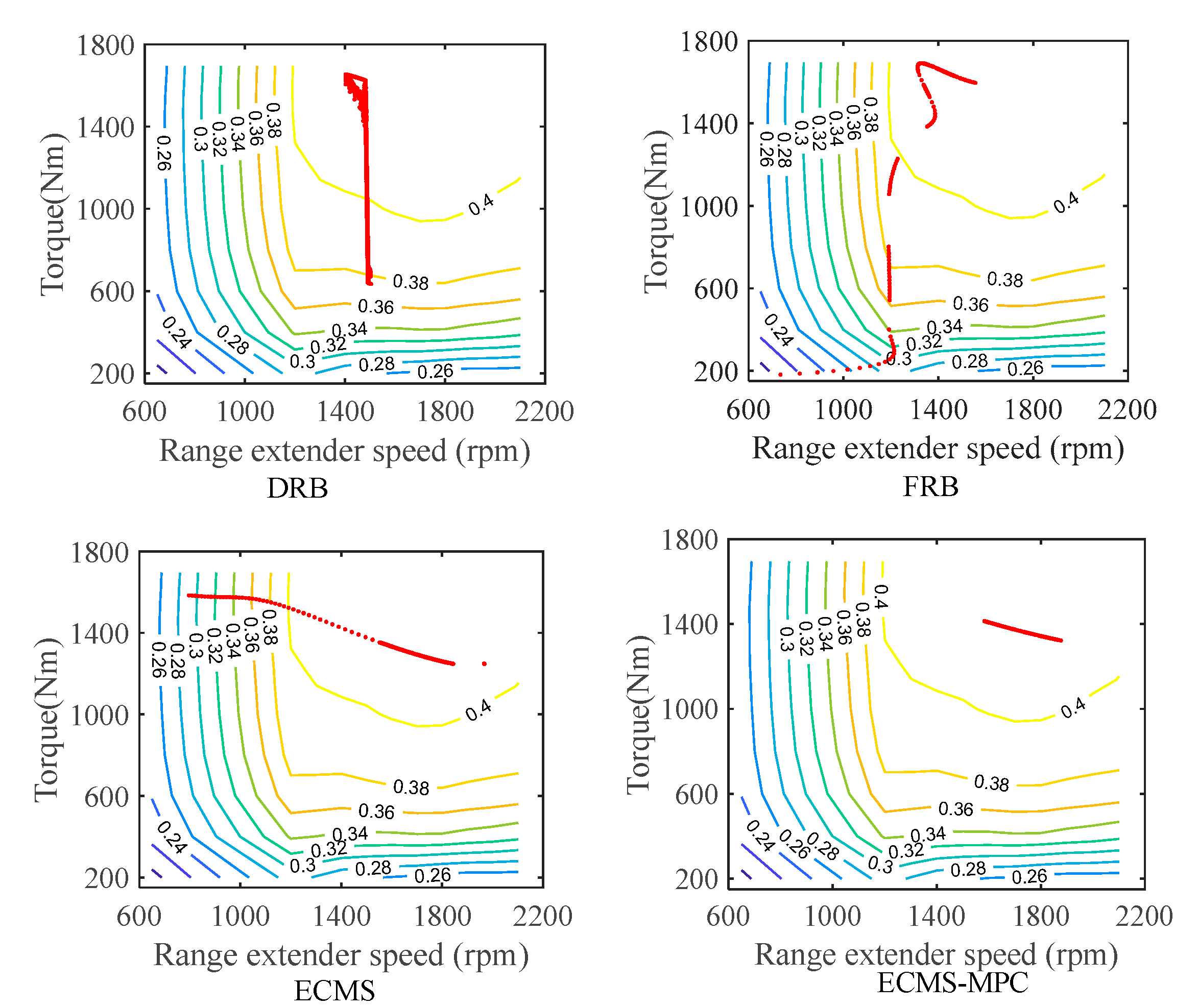
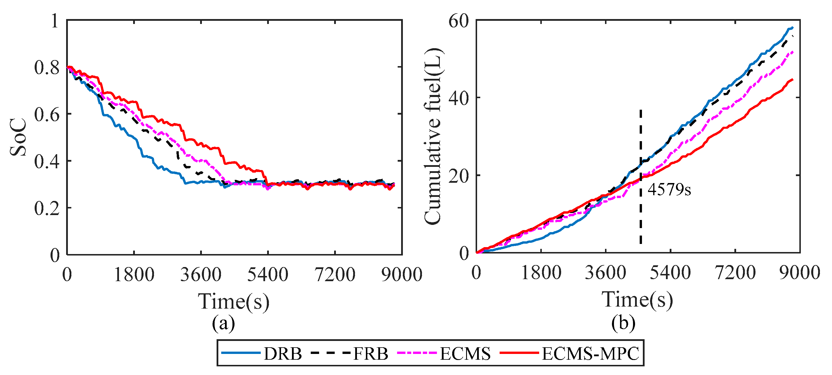
5.3.2. Performance Analysis

After confirming the τ and k ^ , the ECMS-MPC was used to optimize the fuel consumption on-line. For verifying the effectiveness of the proposed EMS, the performances of the DRB EMS, FRB EMS, ECMS and ECMS-MPC were comparatively analyzed under the same simulation environment and vehicle parameters. The heavy-duty transportation and empty-vehicle going-down-mine cycle in Figure 14 were regarded as a whole working cycle, and we selected four cycles to simulate on the HIL platform. Considering the capacity and characteristics of the lithium iron phosphate battery for the SHE-MT studied in this paper, the SoC initial value SoC max and its expectantly terminal value SoC min were set to 0.8 and 0.3, respectively. Through the simulation experiments, the real-time s * and p curve of the proposed ECMS-MPC are displayed in Figure 16. The assigned P re * and P b * profiles of the four EMSs are indicated in Figure 17.
First, when the vehicle respectively produced the assigned P re * and P b * of the four EMSs, as shown in Figure 17, the speed-following effects of the four EMSs were determined, as shown in Figure 18. It can be seen that the speed changing trends of the four EMSs can effectively follow the changing trend of the desired speed.
Then, as shown in Figure 17, the four EMSs, due to adopting different optimization methods, made the variations in P re * and P b * curves different. Correspondingly, the operating points distributions of the range extender were also different, as shown in Figure 19. Compared to the other three EMSs, the operation points of the proposed ECMS-MPC can be more focused on the high-efficiency zone. Accordingly, the SoC and fuel consumption curves of the four EMSs are shown in Figure 20. It can be seen that though the SoC thresholds of the four strategies were capable up to the set terminal value of 0.3, due to the different optimization methods, they resulted in significant differences in the fuel-saving effect.
Specifically, as shown in Figure 20, before the time of 4579 s, compared to the proposed ECMS-MPC, the DRB EMS, FRB EMS, and ECMS were more inclined to use electric energy, making their fuel consumption less than that of the ECMS-MPC. However, with the increase in the vehicle running time, because the proposed ECMS-MPC was solved by local optimization method, its fuel-saving effect was gradually better than that of the other three EMSs. The cumulative fuel consumption rates of the four EMSs are shown in Table 4. Meanwhile, the cumulative fuel consumption rates of the internal combustion engine mine truck (ICE-MT) was also considered. Contrasting with the ICE-MT, DRB, FRB and ECMS, the fuel consumption of the ECMS-MPC was reduced by 38.36%, 23.15%, 19.96%, and 13.63%, respectively.
As mentioned above, on the premise of ensuring the real-time performance and speed-tracking effect, the proposed ECMS-MPC can real-time adjust the EF by means of the MPC method. Compared to the existing real-time EMSs, it had better energy management performance, providing a new solution for the on-line optimization of energy consumption of SHE-MTs.

6. Conclusions

This paper proposes an ECMS-MPC for the minimum fuel consumption of SHE-MTs. First of all, for achieving the on-line speed trajectory, the proposed EMS built an RNN speed prediction model based on the GA-PSOA. Then, combining the obtained on-line speed trajectory and establishing a power-optimal fuel consumption mapping model of the range extender, we used the rolling optimization idea of MPC to design the ECMS-MPC, and achieved the optimal EF solution on-line by means of the PSOA. Finally, with the help of the condition data of the cement mine road, experimental research was carried out for the presented ECMS-MPC on the HIL platform.
According to the experimental results analysis, the designed RNN-SPM effectively achieved speed on-line prediction exceeding 98% prediction precision. In comparison to the existing real-time EMSs, while ensuring real-time performance, the ECMS-MPC can further decreased the fuel consumption rate by adopting the rolling optimization method. Specifically, compared to the DRB EMS, FRB EMS and ECMS, it achieved fuel savings of 23.15%, 19.96%, and 13.63%, respectively. This indicates that the designed ECMS-MPC is capable of offering an effective method for the on-line energy management of SHE-MTs.
In the future, we will conduct more in-depth research on our work. At present, the influence of the stochastic factors to the vehicle state has not been considered in the process of designing the strategy. For example, changes in the ambient temperature can influence the battery discharge ability. In the next research step, to further improve the adaptability of the strategy to complex environments, an adaptive EMS without relying on the analytical model of the vehicle will be established.

Author Contributions

J.L. and Y.L. conceived and completed the writing of the manuscript. Z.C. made key modifications to important knowledge parts. H.Y. assisted with the code design and experimental analysis. All authors have read and agreed to the published version of the manuscript.

Funding

This research was supported by the Young Scientists Fund of the National Natural Science Foundation of China (Grant No. 62103415).

Data Availability Statement

The data presented in this study are available upon request from the corresponding author. The data are not publicly available because the supporting project has a confidentiality agreement.

Acknowledgments

The authors would like to thank the editor and reviewers for their valuable comments and suggestions, which helped them improve the manuscript.

Conflicts of Interest

The authors declare no competing financial interests.

Abbreviations

ECMSequivalent consumption minimization strategy
SHE-MTsseries hybrid electric mine trucks
RNNrecurrent neural network
GAgenetic algorithm
PSOAparticle swarm optimization algorithm
MPCmodel predictive control
EFequivalent factor
ECMS-MPCECMS based on MPC
EMSsenergy management strategies
RBrule-based
CDCScharge-sustaining
DRBdeterministic RB
FRBfuzzy RB
SoCstate of charge
PMPPontryagin’s minimum principle
DPdynamic programming
BPNNbackpropagation neural network
P re m ˙ e * power P re —optimal fuel consumption m ˙ e *
HILhardware-in-loop
VCUvehicle control unit
KAMkinematics analysis method
BPNN-SPMBPNN speed prediction method
RNN-SPMRNN speed prediction method based on GA-PSOA
ICE-MTinternal combustion engine mine truck
Variables and Its Unit
VariablesNameUnit
T wh ( t ) demand torque of the wheelNm
n wh ( t ) speed of the wheelr/min
P wh ( t ) power of the wheelkW
t discrete times
m v vehicle masskg
ggravity accelerationm/s2
θslope angle°
ρ f rolling resistance coefficient
δrotational mass conversion coefficient
αaccelerationm/s2
CDair resistance coefficient
Afrontal aream2
ρ a air densitykg/m3
vvehicle speedm/s
rwhwheel radiusm
P re output power of the range extenderkW
P g electric power of the generatorkW
m ˙ e engine fuel consumption rateg/kwh
T re torque of the range extenderNm
n re speed of the range extenderr/min
P e output mechanical power of the enginekW
T e output torque of the engineNm
n e output speed of the enginer/min
m e fuel consumption of the range extenderg
U g voltage of the generatorV
I g current of the generatorA
T g input torque of the generatorNm
n g input speed of the generatorr/min
i eg mechanical transmission efficiency between the engine and generator
i g generating efficiency of the generator
i re efficiency of the range extender
U b terminal voltage of the battery backV
R b internal resistance of the battery backohm
C Ah capacity of the battery backAh
P b output electric power of the battery packkW
I b loop current of the battery packA
i ch charging efficiency of the battery pack
i dis discharging efficiency of the battery pack
P m output mechanical powerkW
T m output torque of the driving motorNm
n m output speed of the driving motorr/min
U m voltage of the driving motor V
I m current of the driving motorA
i m converting efficiency of driving motor between the mechanical and electric energy
i d driving efficiency of the drive assembly
i f speed ratio of the drive assembly
J total fuel consumption of whole tripg
m ˙ f _ eqv equivalent fuel consumption ratiog/s
Q lhv fuel calorific valueJ/g
t 0 start moment of driving conditions
t f end moment of driving conditions
s EF
p penalty factor
τ preview window size
u * optimal control sequence at discrete time t
u * optimal power combination of the range extender and battery pack at each discrete moment
P re * optimal power of range extenderkW
P b * optimal power of battery packkW

References

  1. He, X.; Jiang, Y. Review of hybrid electric systems for construction machinery. Autom. Constr. 2018, 92, 286–296. [Google Scholar] [CrossRef]
  2. Tong, Z.-M.; Miao, J.-Z.; Li, Y.-S.; Tong, S.-G.; Zhang, Q.; Tan, G.-R. Development of electric construction machinery in China: A review of key technologies and future directions. J. Zhejiang Univ. Sci. 2021, 22, 245–264. [Google Scholar] [CrossRef]
  3. Liu, T.; Yu, H.; Guo, H.; Qin, Y.; Zou, Y. Online Energy Management for Multimode Plug-In Hybrid Electric Vehicles. IEEE Trans. Ind. Inform. 2019, 15, 4352–4361. [Google Scholar] [CrossRef]
  4. Buccoliero, G.; Anselma, P.G.; Bonab, S.A.; Belingardi, G.; Emadi, A. A New Energy Management Strategy for Multimode Power-Split Hybrid Electric Vehicles. IEEE Trans. Veh. Technol. 2019, 69, 172–181. [Google Scholar] [CrossRef]
  5. Liu, J.; Chen, Y.; Li, W.; Shang, F.; Zhan, J. Hybrid-Trip-Model-Based Energy Management of a PHEV With Computation-Optimized Dynamic Programming. IEEE Trans. Veh. Technol. 2017, 67, 338–353. [Google Scholar] [CrossRef]
  6. Hofman, T.; Steinbuch, M.; Van Druten, R.; Serrarens, A. Rule-based energy management strategies for hybrid vehicles. Int. J. Electr. Hybrid Veh. 2007, 1, 71. [Google Scholar] [CrossRef]
  7. Zulkifli, S.A.; Saad, N.; Aziz, A.R.A. Deterministic and fuzzy logic control of through-the-road split-parallel hybrid electric vehicle. In Proceedings of the 2016 International Conference on Computational Science and Computational Intelligence (CSCI), Las Vegas, NV, USA, 15–17 December 2016; pp. 169–174. [Google Scholar] [CrossRef]
  8. Chen, J.; Xu, C.; Wu, C.; Xu, W. Adaptive Fuzzy Logic Control of Fuel-Cell-Battery Hybrid Systems for Electric Vehicles. IEEE Trans. Ind. Inform. 2016, 14, 292–300. [Google Scholar] [CrossRef]
  9. Jalil, N.; Kheir, N.A.; Salman, M. Rule-based energy management strategy for a series hybrid vehicle. In Proceedings of the American Control Conference, Albuquerque, NM, USA, 6 June 1997; Volume 1, pp. 689–693. [Google Scholar]
  10. Wen, Q.; Wang, F.; Xu, B.; Sun, Z. Improving the Fuel Efficiency of Compact Wheel Loader with a Series Hydraulic Hybrid Powertrain. IEEE Trans. Veh. Technol. 2020, 69, 10700–10709. [Google Scholar] [CrossRef]
  11. Zhao, D.; Zhang, Z.; Li, T.; Lan, H.; Zhang, M.; Dong, Y. Fuzzy logic control strategy of series hybrid power loader. J. Jilin Univ. Eng. Technol. Ed. 2014, 44, 1334–1341. [Google Scholar] [CrossRef]
  12. Wu, J.; Ruan, J.; Zhang, N.; Walker, P.D. An Optimized Real-Time Energy Management Strategy for the Power-Split Hybrid Electric Vehicles. IEEE Trans. Control Syst. Technol. 2018, 27, 1194–1202. [Google Scholar] [CrossRef]
  13. Liu, J.; Chen, Y.; Zhan, J.; Shang, F. Heuristic Dynamic Programming Based Online Energy Management Strategy for Plug-In Hybrid Electric Vehicles. IEEE Trans. Veh. Technol. 2019, 68, 4479–4493. [Google Scholar] [CrossRef]
  14. Liu, J.; Chen, Y.; Zhan, J.; Shang, F. An On-Line Energy Management Strategy Based on Trip Condition Prediction for Commuter Plug-In Hybrid Electric Vehicles. IEEE Trans. Veh. Technol. 2018, 67, 3767–3781. [Google Scholar] [CrossRef]
  15. Paganelli, G.; Guerra, T.M.; Delprat, S.; Santin, J.-J.; Delhom, M.; Combes, E. Simulation and assessment of power control strategies for a parallel hybrid car. Proc. Inst. Mech. Eng. Part D J. Automob. Eng. 2000, 214, 705–717. [Google Scholar] [CrossRef]
  16. Sciarretta, A.; Back, M.; Guzzella, L. Optimal Control of Parallel Hybrid Electric Vehicles. IEEE Trans. Control Syst. Technol. 2004, 12, 352–363. [Google Scholar] [CrossRef]
  17. Sezer, V.; Gokasan, M.; Bogosyan, S. A Novel ECMS and Combined Cost Map Approach for High-Efficiency Series Hybrid Electric Vehicles. IEEE Trans. Veh. Technol. 2011, 60, 3557–3570. [Google Scholar] [CrossRef]
  18. Zhang, Y.; Chu, L.; Fu, Z.; Xu, N.; Guo, C.; Zhang, X.; Chen, Z.; Wang, P. Optimal energy management strategy for parallel plug-in hybrid electric vehicle based on driving behavior analysis and real time traffic information prediction. Mechatronics 2017, 46, 177–192. [Google Scholar] [CrossRef]
  19. Li, L.; You, S.; Yang, C.; Yan, B.; Song, J.; Chen, Z. Driving-behavior-aware stochastic model predictive control for plug-in hybrid electric buses. Appl. Energy 2016, 162, 868–879. [Google Scholar] [CrossRef]
  20. Han, J.; Shu, H.; Tang, X.; Lin, X.; Liu, C.; Hu, X. Predictive energy management for plug-in hybrid electric vehicles considering electric motor thermal dynamics. Energy Convers. Manag. 2021, 251, 115022. [Google Scholar] [CrossRef]
  21. Nilsson, T.; Fröberg, A.; Åslund, J. Predictive control of a diesel electric wheel loader powertrain. Control Eng. Pract. 2015, 41, 47–56. [Google Scholar] [CrossRef]
  22. Xie, S.; He, H.; Peng, J. An energy management strategy based on stochastic model predictive control for plug-in hybrid electric buses. Appl. Energy 2017, 196, 279–288. [Google Scholar] [CrossRef]
  23. Wu, J.; He, H.; Peng, J.; Li, Y.; Li, Z. Continuous reinforcement learning of energy management with deep Q network for a power split hybrid electric bus. Appl. Energy 2018, 222, 799–811. [Google Scholar] [CrossRef]
  24. Liu, T.; Hu, X.; Hu, W.; Zou, Y. A Heuristic Planning Reinforcement Learning-Based Energy Management for Power-Split Plug-in Hybrid Electric Vehicles. IEEE Trans. Ind. Inform. 2019, 15, 6436–6445. [Google Scholar] [CrossRef]
  25. Wu, Y.; Tan, H.; Peng, J.; Zhang, H.; He, H. Deep reinforcement learning of energy management with continuous control strategy and traffic information for a series-parallel plug-in hybrid electric bus. Appl. Energy 2019, 247, 454–466. [Google Scholar] [CrossRef]
  26. Sun, C.; Sun, F.; He, H. Investigating adaptive-ECMS with velocity forecast ability for hybrid electric vehicles. Appl. Energy 2017, 185, 1644–1653. [Google Scholar] [CrossRef]
  27. Li, J.; Liu, Y.; Qin, D.; Li, G.; Chen, Z. Research on Equivalent Factor Boundary of Equivalent Consumption Minimization Strategy for PHEVs. IEEE Trans. Veh. Technol. 2020, 69, 6011–6024. [Google Scholar] [CrossRef]
  28. Gu, B.; Rizzoni, G. An Adaptive Algorithm for Hybrid Electric Vehicle Energy Management Based on Driving Pattern Recognition. In Proceedings of the ASME International Mechanical Engineering Congress and Exposition, Chicago, IL, USA, 5–10 November 2006; pp. 249–258. [Google Scholar] [CrossRef]
  29. Guo, H.; Sun, Q.; Wang, C.; Wang, Q.; Lu, S. A systematic design and optimization method of transmission system and power management for a plug-in hybrid electric vehicle. Energy 2018, 148, 1006–1017. [Google Scholar] [CrossRef]
  30. Kazemi, H.; Fallah, Y.P.; Nix, A.; Wayne, S. Predictive AECMS by Utilization of Intelligent Transportation Systems for Hybrid Electric Vehicle Powertrain Control. IEEE Trans. Intell. Veh. 2017, 2, 75–84. [Google Scholar] [CrossRef]
  31. Richalet, J.; Abu El Ata-Doss, S.; Delineau, L.; Estival, J.; Butler, H. Model based predictive control of exotic systems. In Proceedings of the IFAC Symposia Series-Proceedings of a Triennial World Congress, Tallinn, Finland, August 1990; pp. 249–256. [Google Scholar] [CrossRef]
  32. Fu, K.S. Learning control systems and intelligent control systems. An intersection of artificial intelligence and automatic control. IEEE Trans. Autom. Control 1971, 16, 70–72. [Google Scholar] [CrossRef]
  33. Zhang, X.; Yang, L.; Sun, X.; Jin, Z.; Xue, M. ECMS-MPC Energy Management Strategy for Plug-In Hybrid Electric Buses Considering Motor Temperature Rise Effect. IEEE Trans. Transp. Electrif. 2022, 9, 210–221. [Google Scholar] [CrossRef]
  34. Xie, H.; Tian, G.; Du, G.; Huang, Y.; Chen, H.; Zheng, X.; Luan, T.H. A Hybrid Method Combining Markov Prediction and Fuzzy Classification for Driving Condition Recognition. IEEE Trans. Veh. Technol. 2018, 67, 10411–10424. [Google Scholar] [CrossRef]
  35. Vadamalu, R.S.; Beidl, C. Explicit MPC PHEV energy management using Markov chain based predictor: Development and validation at Engine-In-The-Loop testbed. In Proceedings of the 2016 European Control Conference, ECC 2016, Aalborg, Denmark, 29 June–1 July 2016; pp. 453–458. [Google Scholar] [CrossRef]
  36. Levin, E. A recurrent neural network: Limitations and training. Neural Netw. 1990, 3, 641–650. [Google Scholar] [CrossRef]
  37. Bao, X.; Sun, Z.; Sharma, N. A recurrent neural network based MPC for a hybrid neuroprosthesis system. In Proceedings of the 2017 IEEE 56th Annual Conf. on Decision and Control (CDC), Melbourne, VIC, Australia, 12–15 December 2017; pp. 4715–4720. [Google Scholar] [CrossRef]
  38. Hagan, M.T.; Demuth, H.B.; Beale, M. Neural Network Design; China Machine Press: Beijing, China, 2002. [Google Scholar]
  39. Michalewicz, Z.; Vignaux, G.A.; Hobbs, M. A Nonstandard Genetic Algorithm for the Nonlinear Transportation Problem. ORSA J. Comput. 1991, 3, 307–316. [Google Scholar] [CrossRef]
  40. Yu, Z.; Dawei, M.; Meilan, Z.; Dengke, L. Management Strategy Based on Genetic Algorithm Optimization for PHEV. Int. J. Control Autom. 2014, 7, 399–408. [Google Scholar] [CrossRef]
  41. Kennedy, J.; Eberhart, R. Particle Swarm Optimization. In Proceedings of the ICNN’95—International Conference on Neural Networks, Perth, Australia, 27 November–1 December 1995; Volume 4, pp. 1942–1948. [Google Scholar] [CrossRef]
  42. Zhang, W.; Hao, Z.; Zhu, J.; Du, T.; Hao, H. BP neural network model for short-time traffic flow forecasting based on trans-formed grey wolf optimizer algorithm. Transp. Syst. Eng. Inf. 2020, 20, 196–203. [Google Scholar] [CrossRef]
  43. Yang, Z.-L.; Guo, X.-Q.; Chen, Z.-M.; Huang, Y.-F.; Zhang, Y.-J. RNN-Stega: Linguistic Steganography Based on Recurrent Neural Networks. IEEE Trans. Inf. Forensics Secur. 2018, 14, 1280–1295. [Google Scholar] [CrossRef]
  44. Wang, D.; Zou, Y.; Tao, Y.; Wang, B. Password guessing based on recurrent neural networks and generative adversarial net-works. Jisuanji Xuebao/Chin. J. Comput. 2021, 44, 1519–1534. [Google Scholar] [CrossRef]
  45. Chen, F.-C. Back-propagation neural networks for nonlinear self-tuning adaptive control. IEEE Control Syst. Mag. 1990, 10, 44–48. [Google Scholar] [CrossRef]
Figure 1. Power topology of the SHE-MT.
Energies 16 03942 g001
Figure 2. The mapping characteristics. (a) The fuel map of range extender. (b) The efficiency map of range extender. (c) The motor map.
Energies 16 03942 g002
Figure 3. (a) The MPC idea. (b) The prediction principle of speed.
Energies 16 03942 g003
Figure 4. RNN structure. (a) General structure of RNN. (b) Speed prediction model topology of RNN.
Energies 16 03942 g004
Figure 5. The training process of the RNN speed prediction method based on the GA−PSOA.
Energies 16 03942 g005
Figure 6. Online prediction of vehicle speed.
Energies 16 03942 g006
Figure 7. The real-time training principle of the speed prediction model.
Energies 16 03942 g007
Figure 8. The realization framework of the ECMS-MPC.
Energies 16 03942 g008
Figure 9. The selected route.
Energies 16 03942 g009
Figure 10. The vehicle condition information. (a) Collected vehicle speed information. (b) Collected acceleration information. (c) Collected slope angle information.
Energies 16 03942 g010
Figure 11. The simulation platform.
Energies 16 03942 g011
Figure 12. Relationship between iterations and average fitness values of three algorithms.
Energies 16 03942 g012
Figure 13. Selection of τ and k ^ . (a) The relationship between prediction M A E and τ . (b) The relationship between training time and k ^ .
Energies 16 03942 g013
Figure 14. The speed prediction results. (a) The predictive and actual speed curves of three methods. (b) of three methods between the predictive and actual speed curves.
Energies 16 03942 g014
Figure 15. Relationship between calculation time and cumulative fuel of the ECMS-MPC with τ .
Energies 16 03942 g015
Figure 16. Real-time s * and p curve. (a) Real-time s * . (b) p curve.
Energies 16 03942 g016
Figure 17. P re * and P b * curves. (a) P re * curves. (b) P b * curves.
Energies 16 03942 g017
Figure 18. Speed-following effects of four EMSs.
Energies 16 03942 g018
Figure 19. The operating point distributions of the range extender of the four EMSs.
Energies 16 03942 g019
Figure 20. SoC and fuel curves of the four EMSs. (a) SoC curves, (b) fuel curves.
Energies 16 03942 g020
Table 1. The parameters of SHE-MT.
TypeDescription
Vehicle body m v = 43,000   kg ;   A = 16   m 2 ; C D = 0.8 ;   r wh = 0.737   m ;   id = 0.9; ρf = 0.02;
Engine2100 rpm@1695 Nm
Motor3500 rpm@3000 Nm
Generator2200 rpm@2000 Nm
BatteryCah = 300 Ah; Ub = 600 V; Rb = 0.2 ohm; idis = ich = 0.96
Other g = 9.81 m / s 2 ;   ρ a = 1.2 kg / m 3 ;   SoC min = 0 . 3 ;   SoC max = 0.8 ;
Table 2. The initial parameters of RNN model.
ParametersInitial Values
U T −1.62−2.30−1.690.311.00
2.401.130.800.821.76
−1.91−0.610.09−2.611.72
W−3.32−0.76−1.68−1.42−3.87
−2.230.841.80−0.22−2.46
−2.16−0.231.15−2.20−1.14
1.842.801.300.86−1.63
0.25−1.44−2.951.722.85
V−1.39−1.63−1.172.763.17
0 T 0.34−1.861.301.37−2.36
Table 3. MAE, RMSE and MRE of the three methods.
CyclePrediction MethodsMAERMSEMRE
Heavy-duty transportation cycleKAM0.26110.01530.0381
BPNN-SPM0.21430.00850.0316
RNN-SPM0.060.00410.0095
Empty-vehicle going-down-mine cycleKAM0.26470.01670.0480
BPNN-SPM0.20160.01080.0351
RNN-SPM0.06180.00450.0105
Table 4. The fuel consumption of the ICE-MT and four EMSs.
EMSsICE-MTDRBFRBECMSECMS-MPC
Initial SoC-0.80.80.80.8
Final SoC-0.30.30.30.3
Fuel (L)72.5558.1955.8751.7844.72
Disclaimer/Publisher’s Note: The statements, opinions and data contained in all publications are solely those of the individual author(s) and contributor(s) and not of MDPI and/or the editor(s). MDPI and/or the editor(s) disclaim responsibility for any injury to people or property resulting from any ideas, methods, instructions or products referred to in the content.

