
FastInformer-HEMS: A Lightweight Optimization Algorithm for Home Energy Management Systems
1
Shanghai Advanced Research Institute, Chinese Academy of Sciences, Shanghai 200120, China
2
University of Chinese Academy of Sciences, Beijing 100049, China
*
Author to whom correspondence should be addressed.
Energies 2023, 16(9), 3897; https://doi.org/10.3390/en16093897
Submission received: 11 March 2023
/
Revised: 25 April 2023
/
Accepted: 2 May 2023
/
Published: 5 May 2023
(This article belongs to the Topic Smart Electric Energy in Buildings)
Abstract
:In a smart home with distributed energy resources, the home energy management system (HEMS) controls the photovoltaic (PV) storage system by executing the optimization algorithm to achieve the lowest power cost. The existing mixed integer linear programming (MILP) algorithm is not suitable for execution on the end-user side due to its high computational complexity. The HEMS algorithm based on a long short-term memory neural network (LSTM-HEMS) can effectively solve the problem of the high computational complexity of MILP, but its optimization outcome is not high due to the accumulation of prediction errors. In order to achieve a better balance between computational complexity and optimization outcome, this paper proposes a lightweight optimization algorithm called the FastInformer-HEMS, which introduces the E-Attn attention mechanism based on Informer and uses global average pooling to extract the attention characteristics. Meanwhile, the proposed method introduces the maximum self-consumption algorithm as a backup strategy to ensure the safe operation of the system. The simulated results show that the computational complexity of the proposed FastInformer-HEMS is the lowest among the existing algorithms. Compared with the existing LSTM-HEMS, the proposed algorithm reduces the power consumption cost by 12.3% and 6.6% in the two typical scenarios, while the execution time decreases by 13.6 times.
1. Introduction
In developed countries and regions, residential areas are responsible for nearly 40% of the energy consumption. Compared to industry and transportation, residential areas have significant potential for energy and cost savings, as well as carbon reduction [1]. In recent years, the increase in the number of distributed power generation devices and controllable electrical appliances has made home energy management systems (HEMS) more complex. Considering the limitations of the operation environment on the end-user side, efficient lightweight optimization algorithms [2] are urgently needed to help residents reduce unnecessary energy consumption and reduce electricity cost.
At present, algorithms applied in home energy system management can be divided into four categories, namely, heuristic algorithms, operational research algorithms, reinforcement learning and machine learning. The heuristic algorithm [3,4,5] obtains a feasible solution for the optimization problem at the cost of an acceptable time and space. Bouakkaz et al. [4] established an optimization model to minimize the energy cost and proposed a particle swarm optimization algorithm to obtain the optimal day-ahead scheduling plan of a battery. Ahmad et al. [5] established an optimization model to minimize energy cost and the peak-to-average ratio and used a genetic algorithm to obtain the optimal day-ahead scheduling of household appliances. Operational research algorithms, such as mixed-integer linear programming (MILP) and dynamic programming, are also applied in home energy management systems. Azuatalam et al. [6] established an MILP model to minimize the cost of electricity for families equipped with PV-storage systems and used the CPLEX solver to establish a day-ahead schedule for appliances. Although the planning results of the methods mentioned above are of high quality, their computational complexity increases exponentially with the number of devices. Moreover, their optimization quality depends on the prediction of future information.
In order to overcome the limitation of the high computational complexity of optimization algorithms mentioned above, early scholars proposed improving methods such as reducing state space [7,8] and reducing MILP scenarios [9]; however, they still could not fundamentally solve the problem of high computational complexity. In this regard, some scholars have introduced reinforcement learning [10,11,12,13] and machine learning [14,15,16,17] methods. Although reinforcement learning has the advantages of not requiring prior knowledge and being less affected by environmental fluctuation, its model is difficult to converge [13]. Huy et al. [14] proposed an hourly demand response strategy based on machine learning, which is directly invoked online after learning the mapping relationship between MILP planning results and the environmental state. The simulated results show that the results of machine learning-based algorithms are better than reinforcement learning. Paridari et al. [18] proposed a plug-and-play algorithm for home energy system management, which adopted a half-hour demand response strategy based on LSTM model and achieved good results. However, it only has a good effect on one-step prediction. Due to the accumulation of errors in multi-step prediction, the prediction accuracy cannot meet the requirements of a demand response strategy. Recently, many scholars have applied the Transformer [19] model in the field of natural language processing to the prediction task of long time series. The Informer model proposed by Zhou et al. [20] realized multi-step prediction and performed well, but its computational complexity still has room to improve.
Given the limited resources on the end-user side, the optimization algorithm for a home energy management system urgently needs to improve the accuracy of multi-step prediction while reducing the computational complexity to continuously improve the optimization outcome. Therefore, we propose a lightweight optimization algorithm for a home energy management system with a PV-storage unit. Based on the Informer model, the network structure and attention mechanism are improved to reduce the computational complexity and improve the optimization benefits. The main contributions of this paper as follows:
- (a)
- A lightweight optimization algorithm called the FastInformer-HEMS is proposed, which introduces the E-Attn attention mechanism [21] and uses global average pooling to extract attention features and improve the accuracy of a battery energy level’s multi-step prediction and effectively reduce the computational complexity.
- (b)
- Considering the need for safe operation, self-consumption maximum (SCM) is introduced as the backup security policy for the first time to ensure that the executed strategy is safe and feasible.
- (c)
- The simulation results show that the proposed algorithm has lower electricity cost than the existing HEMS algorithms, and it has the lowest computational complexity among all algorithms.
2. Background of Home Energy Management
This section introduces the common structure of a home energy system with PV storage, formulates the home energy management optimization problem and finally introduces the algorithm for home energy management based on machine learning.
2.1. Structure of Home Energy System
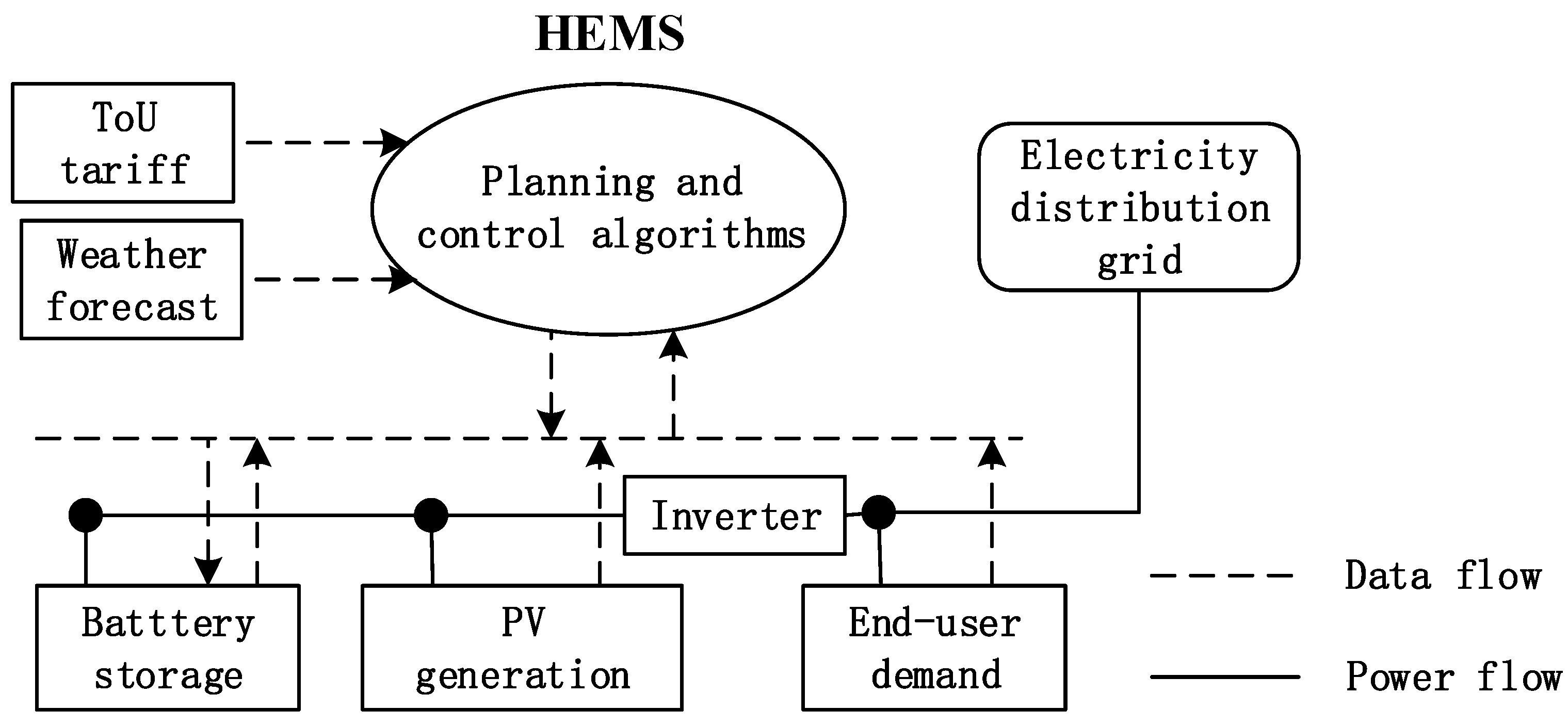
The common structure of a home energy system includes a battery storage unit, PV solar panels and residential appliances. The system structure is shown in Figure 1.
2.2. Home Energy Management Optimization
The goal of home energy management optimization is to minimize a household’s energy costs over a decision horizon. The optimization problem of home energy management system is essentially that an HEMS uses optimization techniques to control the battery or appliances by solving a sequence optimization problem during a decision period (usually 24 h) before the beginning of each day. We consider a simple home energy system, which consists of a photovoltaic power generation unit, a battery storage unit and a corresponding inverter, as depicted in Figure 1 for convenience. Additionally, the specific residential loads are not classified and modeled individually. In this paper, we assume that electricity price is a time-of-use price so that electricity price is not a random variable.
The uncontrollable inputs of the system are power demand, photovoltaic output and electricity price, in which the state variable represents the average load demand, represents the average photovoltaic output, is the electricity tariff, the random variable represents the change of electrical demand, and represents the variations of the PV output. The device controlled by the system is a battery, and the state variable represents the battery SOC (state of charge), while the controllable variable represents the charge and discharge power of the battery.
For each time step, k, in the decision horizon, the system variable set is ,,. The power balance of the system is shown in Formula (1):
where is the inverter power at the DC side, is the conversion efficiency of the inverter, is the charge and discharge efficiency of the battery, and represents the power purchased and sold by the grid. The charge power of the battery meets . The discharge power meets . The battery power is satisfied when .
The system transfer function determines the change of state variables, as shown in Formula (2):
where represents the self-discharge process of the battery. It can be seen from Formula (2) that the multi-step prediction accuracy of battery power directly affects the execution action in the policy for an HEMS.
The optimal strategy, , is a choice of action for each state that minimizes the expected sum of future costs over the decision horizon, as shown in Formula (3):
Here, is the electricity cost in the decision horizon and can be expressed as follows:
Depending on the state variable, or , of each time step, the HEMS obtains the action, x, of the battery, .
2.3. Algorithm Based on Machine Learning for Home Energy Management System
MILP models the HEMS problem as a mathematical programming problem, and the dynamic programming algorithm models the HEMS problem as a Markov decision process. The planning quality of such methods depends on the accurate prediction of PV and the electrical demand. Additionally, their computational costs are high.
In view of the problems mentioned above, a better solution is the home energy management algorithm based on machine learning [18]. The machine learning algorithm is used to realize the mapping of the system state to the decision variable so that the planning result can be obtained quickly with a low computational cost. Additionally, its planning quality does not depend on the accurate prediction of PV and the electrical demand.
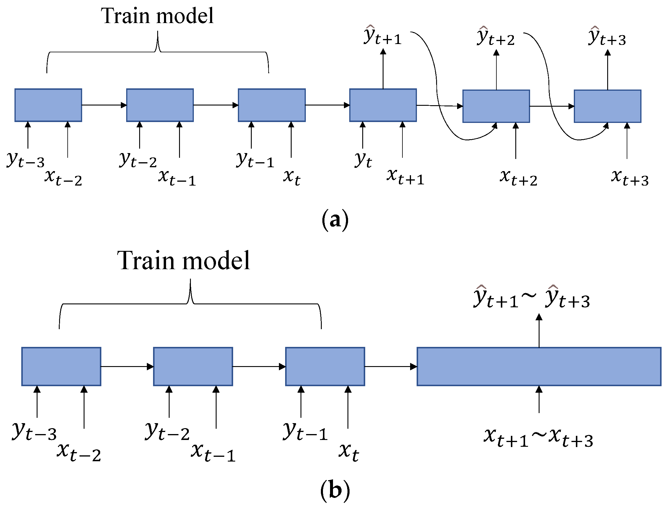
The existing method uses LSTM to predict the decision variables step by step as shown in Figure 2a. There is error accumulation in the decision horizon, which indirectly results in poor planning quality. To solve this problem, we propose a lightweight optimization algorithm, the FastInformer-HEMS, which can reduce computational complexity and improve optimization benefits at the same time.
3. FastInformer-HEMS Algorithm
This section first introduces the overall framework of the optimization algorithm, the FastInformer-HEMS, and then introduces the specific application steps, including the prediction module, security module and strategy generation module, before finally introducing the FastInformer model.
3.1. Algorithm Framework
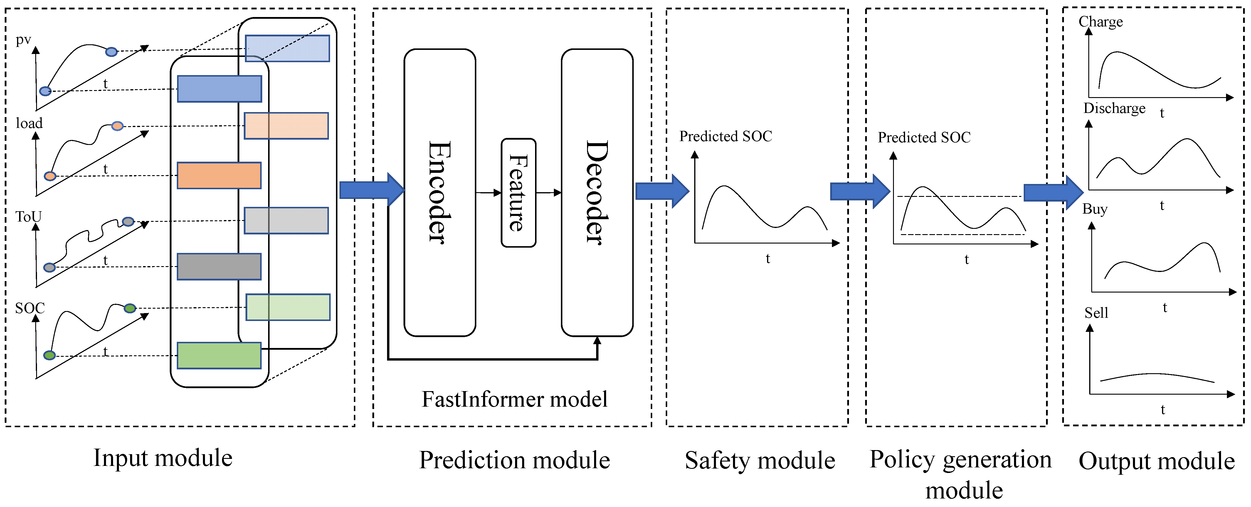
Aiming at the problem of limited resources in end-user side and error accumulation caused by one-step prediction, we introduce the Informer model and propose the FastInformer-HEMS algorithm by improving it. The algorithm first uses the prediction module to realize the multi-step prediction of the battery energy level and then quickly obtains the decision variables via the security module and the strategy generation module. The overall framework is shown in Figure 3.
The prediction module of the algorithm takes the historical photovoltaic output, electrical demand, electricity price and battery power as the inputs of the FastInformer model. After encoding and decoding, the prediction module outputs the battery energy level for a period in the future. The charge or discharge power of the battery and the electrical grid power are calculated by the strategy generation module. Meanwhile, the security module chooses to execute the backup policy to generate feasible action at the time step when the predicted value does not satisfy Formulas (5) and (6).
The formation of the FastInformer-HEMS is described in the following sections.
3.1.1. Prediction Module
The PV generation, electrical demand, time-of-use electricity price and battery power of the previous few days are put into the prediction module, and the proposed multi-step prediction model FastInformer (described in Section 3.2) is used to predict the optimal battery energy level in the next 24 h.
FastInformer first calculates the historical optimal energy level of the battery by using the MILP solver with the household’s historical data, and then the model is trained using the historical environment information as input and the historical optimal solution as the label. Therefore, the trained FastInformer model can output the optimal battery power in the future.
3.1.2. Safety Module
The optimal battery energy level value predicted by the prediction module is used as the input of the safety module, and the SCM is used as the backup safety strategy to filter the predicted value. When the prediction value does not meet the safe operation conditions as shown below, the safety module will choose to perform the backup strategy to ensure the safe operation of the system,
where denotes the predicted value of battery energy level at time step t, denotes the lowest energy level of the battery, denotes the highest energy level of the battery, and represents the upper limit of battery charge or the discharge power.
If does not satisfy the safe operation conditions, the system power gap is calculated as follows, where denotes the inverter efficiency:
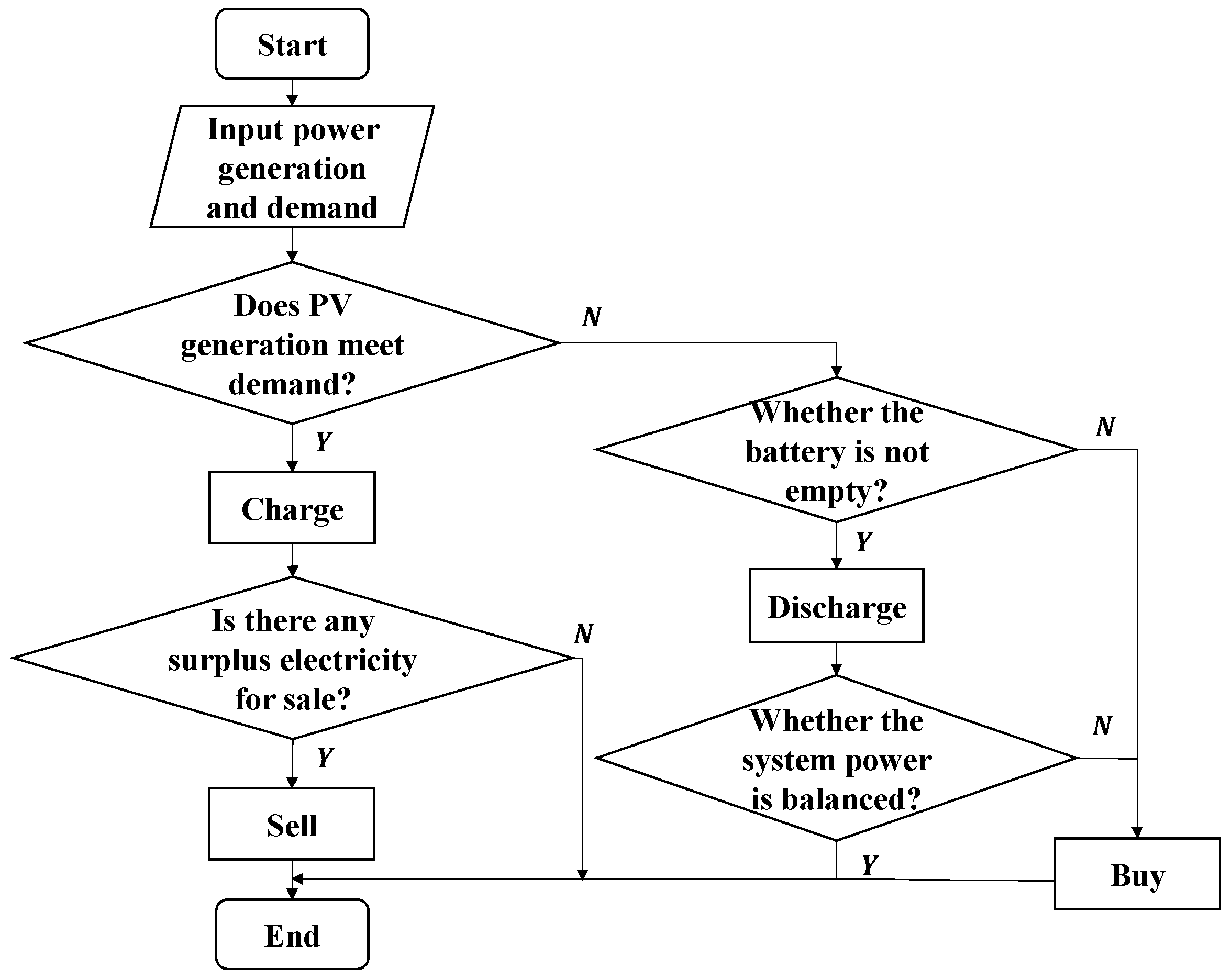
When , it means that the photovoltaic power generation in the current system can meet the electrical demand, and the left PV generation will be charged to the battery or sold to the grid. The battery charging power is calculated as follows, where represents the battery charging or discharging efficiency.
After charging the battery, if there is power left, it will be sold to the grid. The grid power is shown below.
When , it indicates that the photovoltaic generation of the system does not meet the load. According to Equation (2), it is necessary to discharge the battery or buy electricity from the grid to balance the system’s power. The discharge power is calculated as follows:
The system needs to purchase power from the grid as shown below:
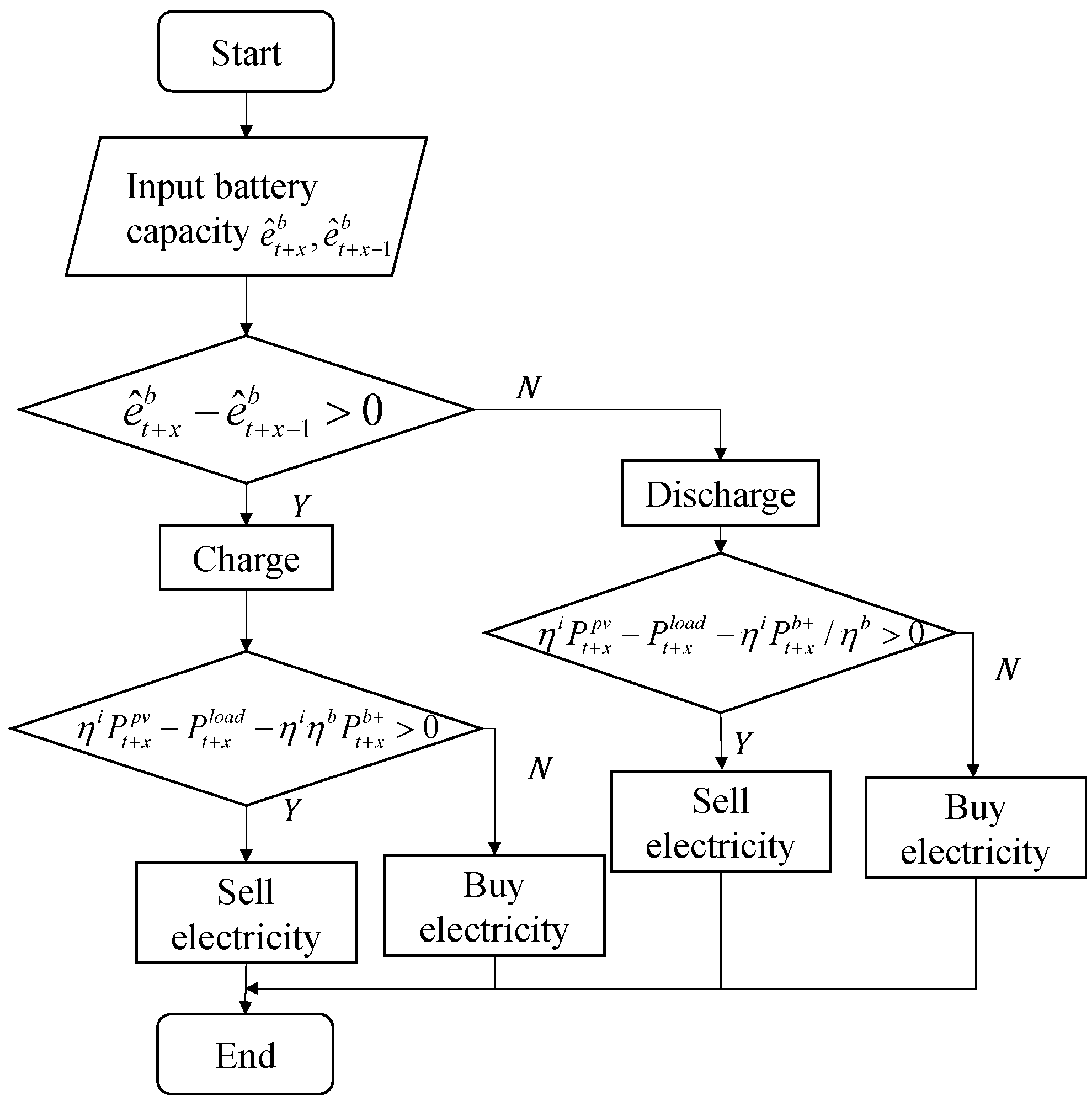
The specific process of the backup safety strategy is shown in Figure 4; that is, the photovoltaic generation and storage battery are preferentially used to meet the load demand and then consider the interaction with the grid.
3.1.3. Strategy Generation Module
The safety module outputs the set of future optimal battery power prediction values that meet the operation requirements. The process of calculating the charging power , discharging power , buying power and selling power at time step t + x is as follows.
According to Formula (2), the power gap between the two time steps, and , can determine the power of buying and selling electricity and the power gap, .
When , the battery needs to be charged, and the charge power is calculated as follows:
After charging the battery, it is necessary to buy or sell electricity to the grid to achieve system power balance. Grid power is calculated as follows.
When , the power of selling electricity , when , the power of buying electricity .
When , the battery needs to be discharged, and the discharge power is calculated as follows:
Similarly, it is necessary to buy or sell electricity from the grid to maintain the power balance of the system. The calculation of is shown in Equation (15):
When , the selling power , when , the buying power .
The strategy generation process is shown in Figure 5.
After calculating the amount of bought electricity or sold electricity, the cost in the decision period can be calculated with the following equation:
where denotes the time-of-use electricity price and denotes the electricity price.
3.2. FastInformer Model
The self-attention mechanism of Transformer makes it perform better than LSTM in long sequence processing. Based on Transformer, Informer [19] adopts a generative decoder to output a long time series in one step, which can solve the problem of error accumulation caused by one-step iterative prediction.
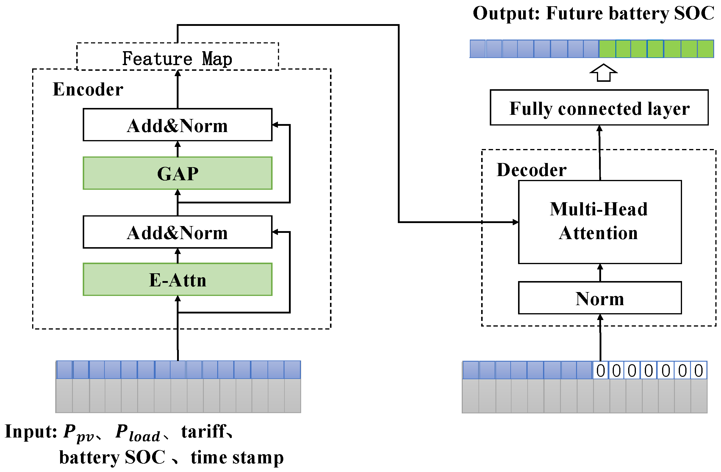
The proposed FastInformer reduces the overall computational complexity of Informer, thus making the HEMS take less time to execute the optimization algorithm. The model is composed of encoder and decoder, and the structure is shown in Figure 6.
3.2.1. Encoder
The encoder is designed to extract useful features from the input so that it can be effectively decoded in the decoder. The encoder layer in Informer is composed of sparse attention module and distillation layer. The proposed FastInformer model introduces E-Attn as the attention module and adopts the global average pooling (GAP) to extract attention features so that its computational complexity is lower than that of Informer.
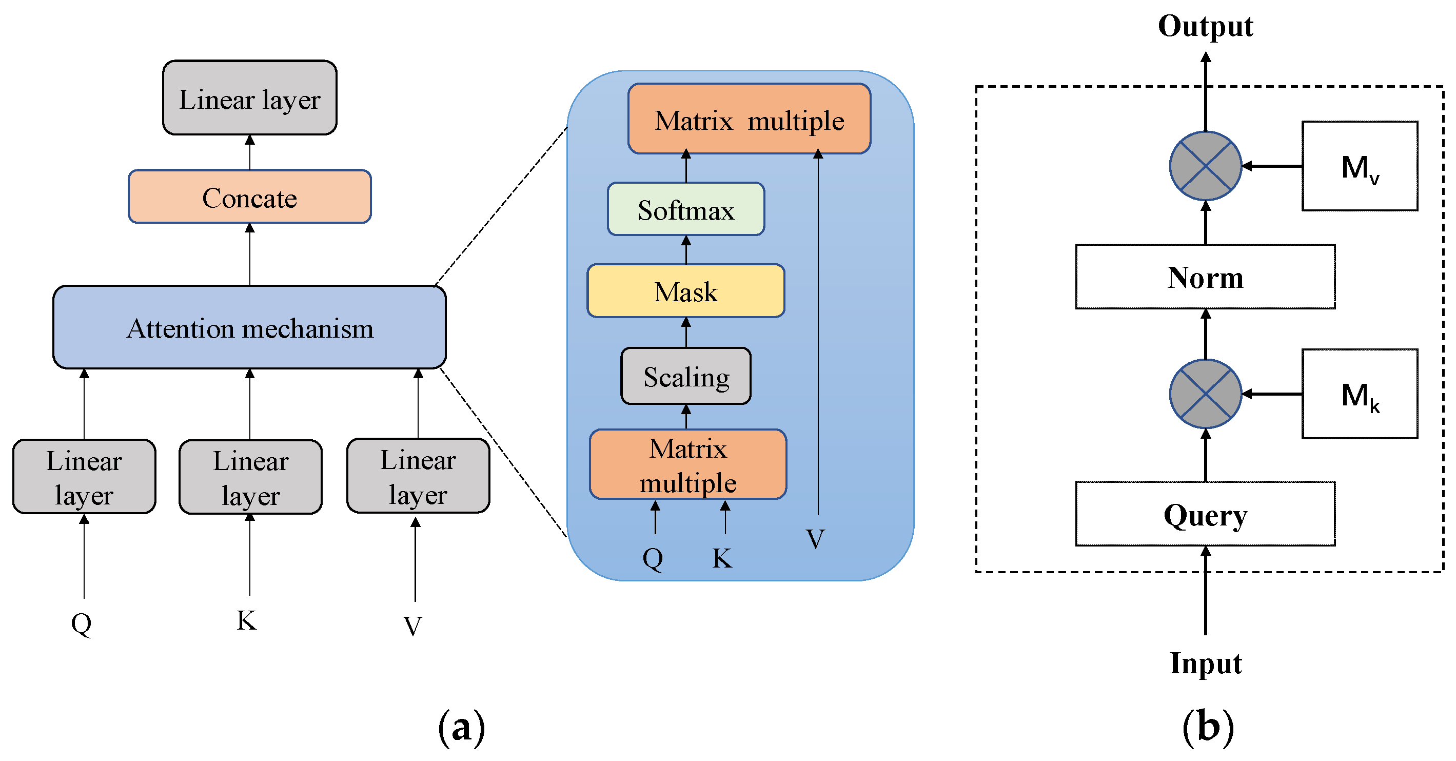
E-Attn attention module is an attention mechanism with linear complexity in visual tasks, which uses two fully connected networks, and , to replace the key and value in attention calculation. This structure is shown in Figure 7.
When denotes the input vector, it becomes vector Q via the fully connected layer, and when the output vector is , the attention calculation formula is shown as follows:
Differently from the original attention mechanism, and are two fully connected layers. In terms of calculating attention, E-Attn attention does not need a matrix multiple so its computational complexity is reduced from to compared to ProbSparse attention, as shown in Figure 6a.
Informer’s encoder adopts multi-layer convolution to extract features after calculating the attention weight. The computational complexity of multi-layer convolution is , where M is the edge length of the output feature map of each convolution core, K is the edge length of each convolution core, and is the th convolution layer. Considering the sparsity of the attention matrix, FastInformer uses the global average pooling to extract the features of the attention matrix, which reduces the computational complexity of this part to O (1).
3.2.2. Decoder
The proposed FastInformer model adopts a generative decoder and adopts the fully connected layer to the output multi-step prediction data at one time, avoiding the error accumulation caused by one-step prediction. In order to reduce the computational complexity of the decoder, the FastInformer decoder only retains the cross-attention module, which reduces the computational complexity of the whole model.
4. Results and Analysis
This section first introduces the data set and experiment settings and then introduces the comparison algorithms and evaluation indicators, before finally verifying the effectiveness of the FastInformer-HEMS in terms of power consumption cost and time consumption in the family scenario of a one-day decision period and a multi-day decision period.
4.1. Dataset
The dataset used is from real data of the smart grid project [22]. This dataset contains electrical demand and PV generation data of customers in Sydney, Australia from 2011 to 2013, belonging to the home energy system described in Section 2.1. The daily decision horizon is a 24 h period divided into 30 min time intervals giving a K = 48 time-step. The information of the energy storage battery used by the household is shown in Table 1.
4.2. Experiment Setup
In order to compare the performance of different algorithms, the experiments are carried out on an NVIDIA GeForce GTX 1080 Ti GPU machine in python environments, and the neural network is built with pytorch. We set the efficiency of the battery as a constant since we tested the policies in a simulated environment instead of a hardware environment. In a real hardware system, the efficiency of the battery and inverter is strictly not linear [23], and we use the constant to approximate the efficiency since we mainly focus on the differences between different policies in our simulated environment. The grid search method is used to determine the model hyperparameters. The model hyperparameter search space of FastInformer is shown in Table 2.
After many experiments, the input length of FastInformer’s encoder is set to 96, the label length of decoder is set to 48, the output length of decoder is 48 and the batch size is 32.
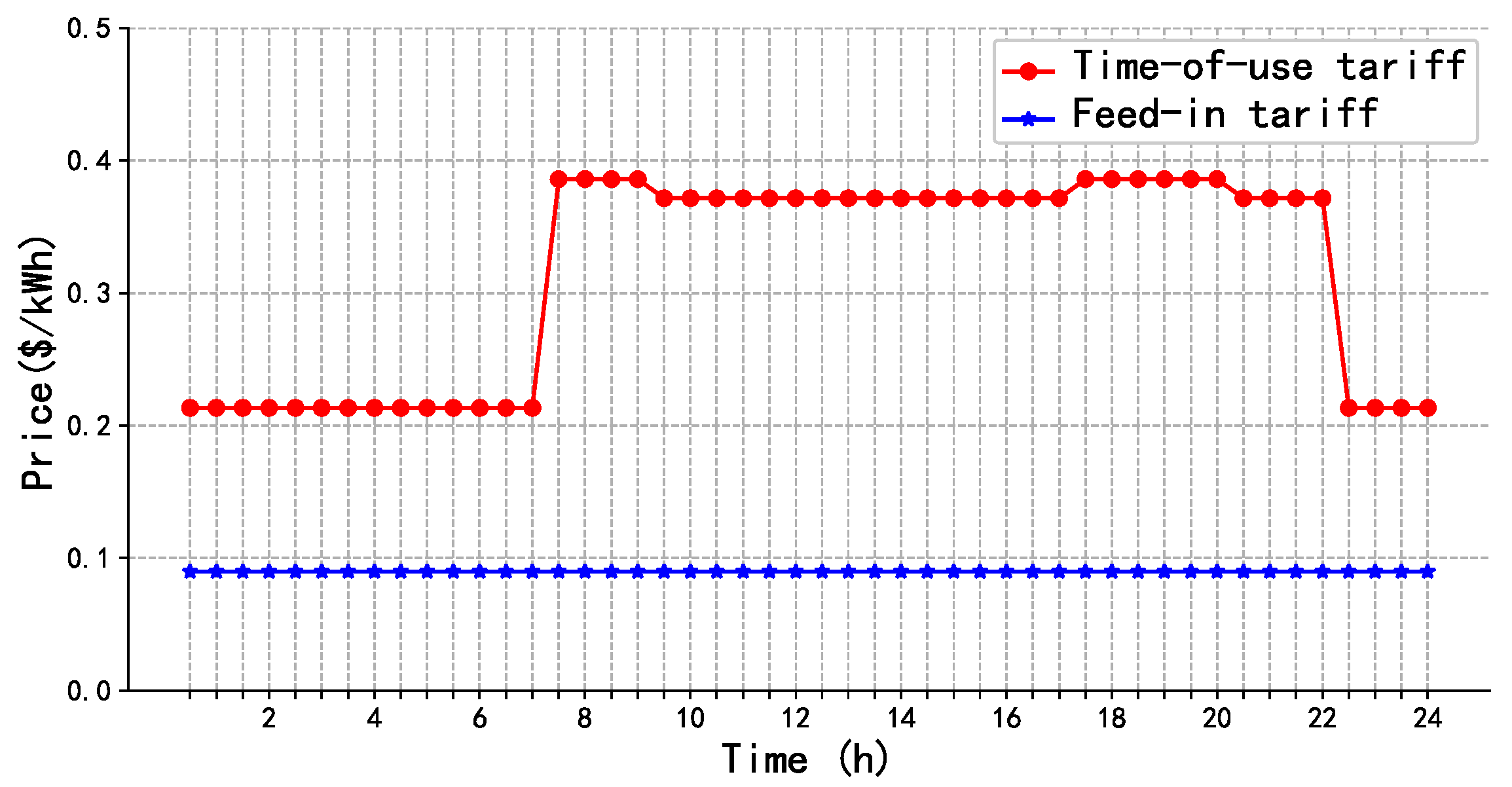
The on-grid electricity price represents the price of selling electricity, and the time-of-use electricity price represents the price of buying electricity from the grid at a different time step. The specific information of time-of-use and feed-in tariff are shown in Figure 8.
4.3. Comparison Algorithm and Evaluation Index
In order to verify the effectiveness of the model, the FastInformer-HEMS is compared with the following three algorithms:
- (a)
- The mixed integer linear programming algorithm (MILP), which assumes that the future PV and load demand are perfectly predictable so that its planning quality is the highest.
- (b)
- The HEMS algorithm based on LSTM (LSTM-HEMS), which is a good choice to avoid the high computational complexity of MILP at present. It adopts the LSTM model to predict decision variables step by step as shown in Figure 2a.
- (c)
- The Informer-based algorithm for an HEMS (Informer-HEMS), which introduces Informer to realize the multi-step prediction of the battery energy level.
In this paper, the electricity cost and execution time in the decision-making horizon are used as the evaluation indicators of each policy. In addition, since the three algorithms based on the neural network all predict the future energy level of the battery first and then obtain the decision variables indirectly, it is necessary to compare the prediction accuracy of the battery’s energy level.
4.4. Analysis of Experiment Results
4.4.1. Quality of Strategies over a Day
In order to compare the execution quality of the three HEMS strategies and MILP in one day, we use the historical data of the same household in the first two years and 240 days from the third year to train the model and use the data after the 241st day in 2013 as the environmental information to simulate the online execution of the strategy.
In order to comprehensively evaluate the performance of the strategies, we compare the execution quality of the strategies over a day in two typical scenarios. In scenario 1, the photovoltaic power generation energy level is large enough to basically meet the household electrical demand. In scenario 2, the photovoltaic generation cannot meet the user demand. In this paper, the 241st and 243rd days are selected as the specific examples of the two typical scenarios for analysis. The information of the scenarios is shown in Table 3.
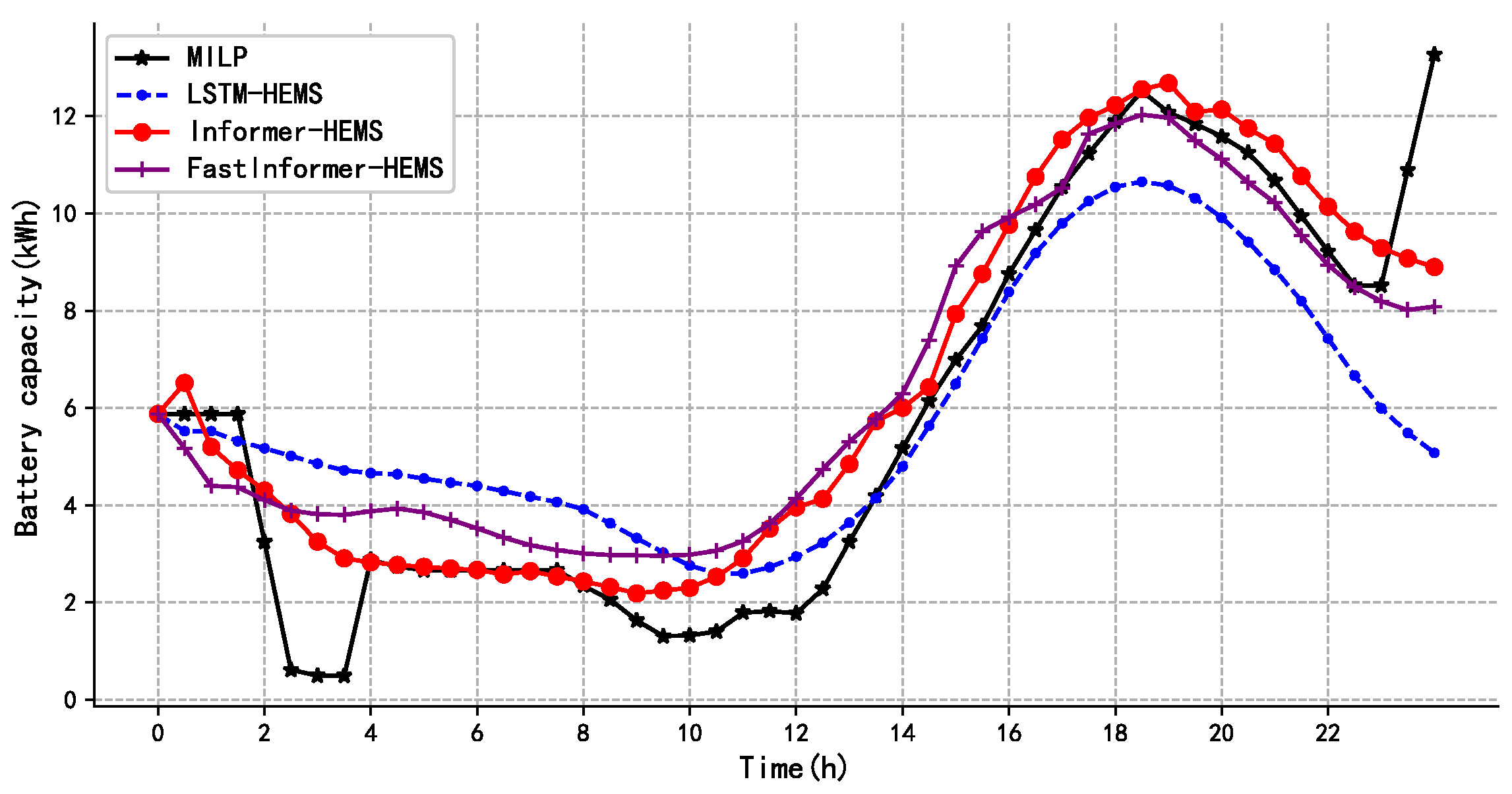
Prediction of Battery’s Energy Level in Two Typical Scenarios
In scenario 1, the photovoltaic power generation capacity basically meets the user’s electrical demand. In order to avoid purchasing power from the grid during the next day’s high electricity price period, the optimal strategy MILP will charge the battery during the low electricity price period, which will reduce the power consumption cost of the next day. As shown in Figure 9, the three HEMS algorithms based on neural networks can all imitate MILP well. Compared to the results of MILP, the average prediction error per time step of the Informer-HEMS is 0.94 kWh, the average error of the FastInformer-HEMS per time step is 1.14 kWh, and the average error of the LSTM-HEMS is 1.64 kWh. The results show that the prediction accuracy of the proposed the FastInformer-HEMS is higher than that of the existing LSTM-HEMS.
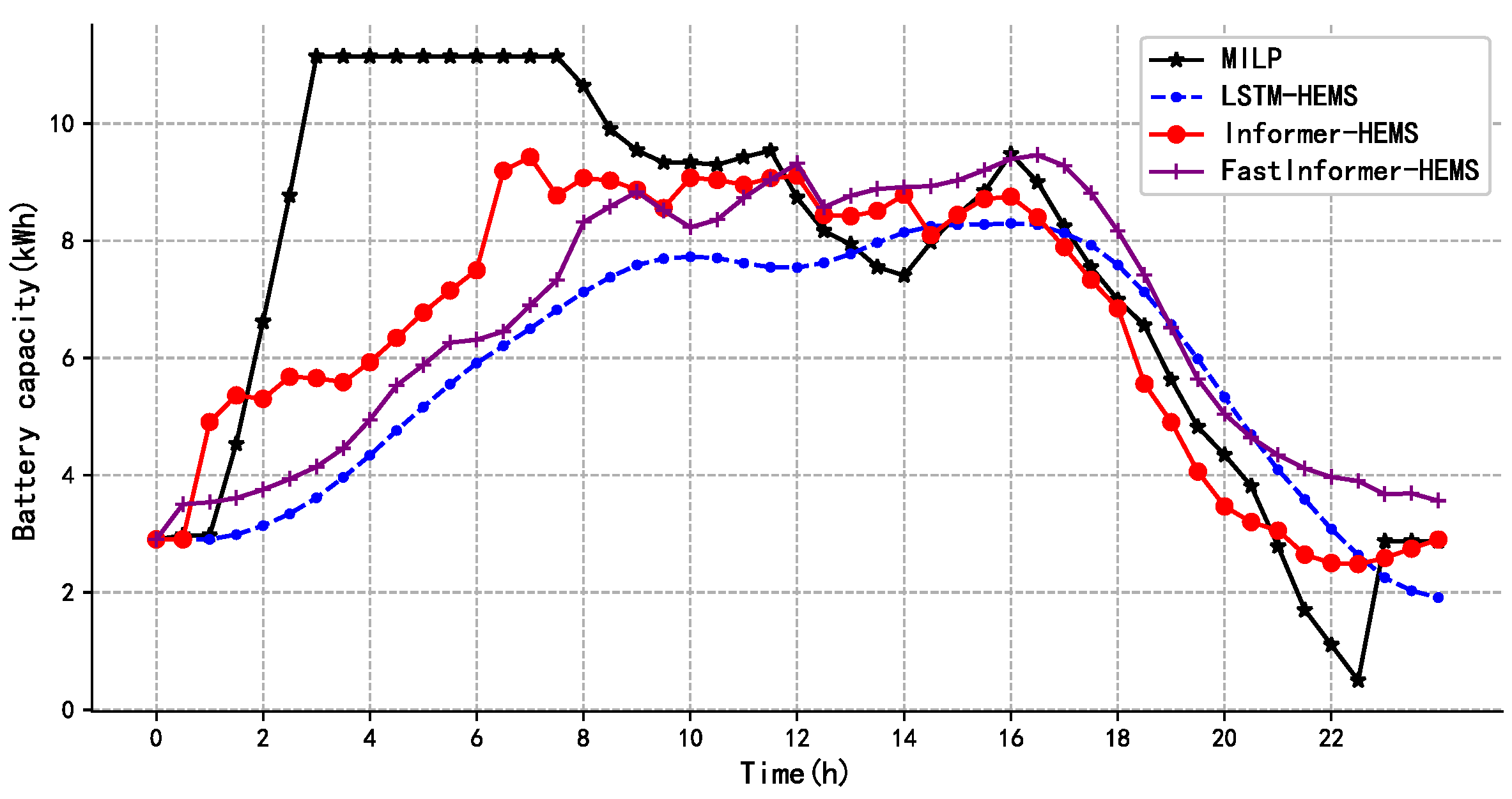
In scenario 2, due to weather and other reasons, the household’s photovoltaic generation cannot meet the electrical demand. In order to reduce the power consumption cost of the day, the perfect optimization of MILP will purchase power at the low electricity price period of the day and discharge the battery in the high electricity price period to meet the electrical demand, thus reducing the power consumption cost. Compared to the LSTM-HEMS, the strategy’s prediction of the battery energy level is closer to MILP, as shown in Figure 10.
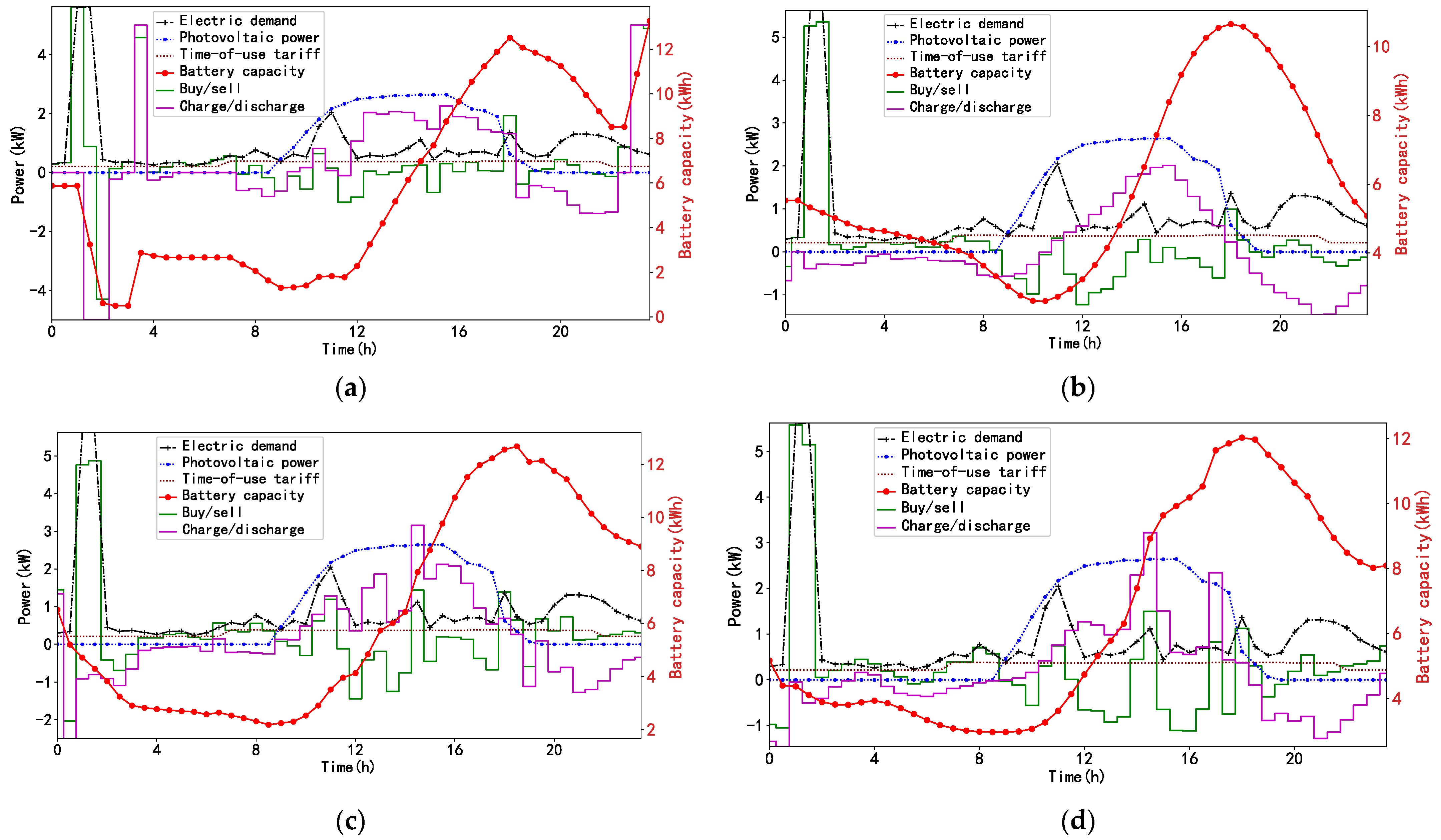
Electricity Costs in Two Typical Scenarios
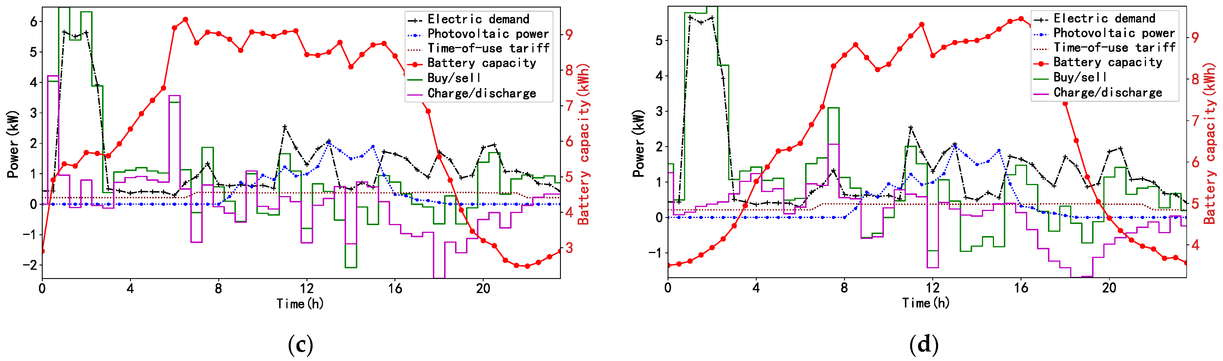
The prediction module outputs the optimal energy level of the battery. Then, the strategy generation module calculates the trading power with the grid and the charge or discharge power of the battery depending on the predicted value. When the predicted value violates the safe operation conditions, the safety module will perform the backup strategy to generate the feasible decision variable. According to the formula in Section 3.1.2 and Section 3.1.3, the charge or discharge power of the battery and the trading power with the grid at each time step can be calculated, as shown in Figure 11. It can be seen from the figure that the FastInformer-HEMS can effectively imitate MILP’s strategy and charge the battery with surplus photovoltaic generation. In addition, the battery is charged in the period of low electricity price, and the battery is preferentially discharged in the period of high electricity price to meet the electrical demand.
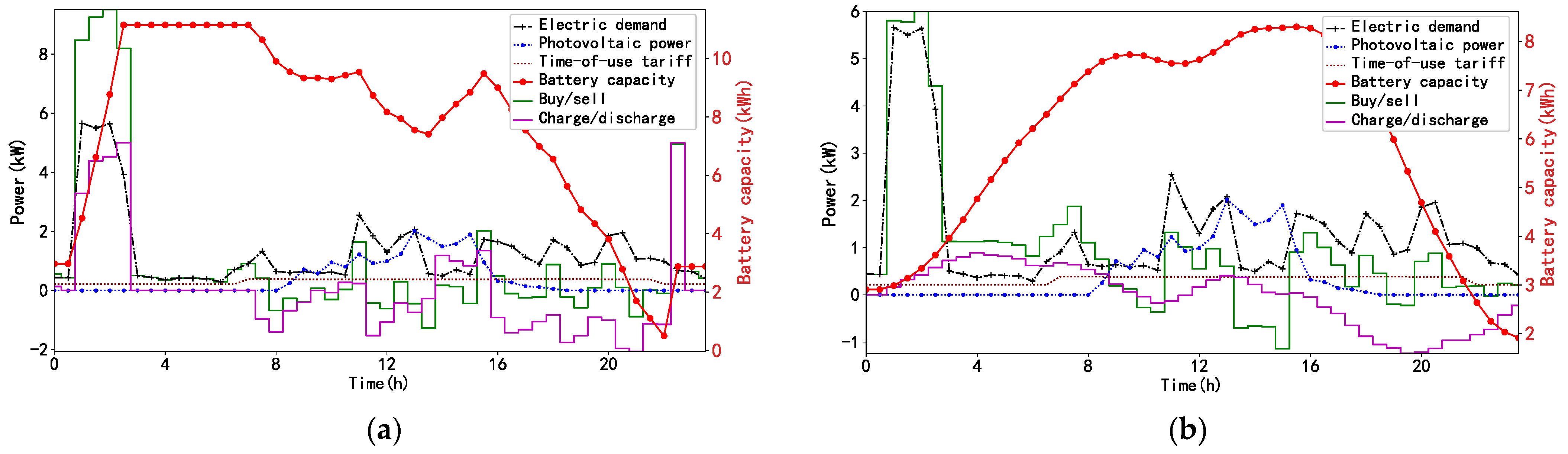
In scenario 2, the optimization results of each policy are shown in Figure 12. Differently from scenario 1, the photovoltaic power generation in scenario 2 cannot meet the power demand, so we need to buy electricity from the grid to maintain the system power balance at most time steps over a decision horizon.
After obtaining the power set of purchasing electricity or selling electricity over a day, the cost over a day is calculated according to Formula (16). The electricity costs in two scenarios are shown in Table 4. Compared with the benchmark, the FastInformer-HEMS reduces the electricity costs to 45.2% and 61.4% in the two scenarios, which is close to the electricity cost of MILP. Compared to the LSTM-HEMS, the FastInformer-HEMS algorithm can reduce the cost by 12.3% and 6.6% in the two typical scenarios. The results show that the proposed algorithm can effectively reduce the electricity cost.
4.4.2. Cost of Strategies over Several Days
In order to fairly evaluate the performance of the different strategies, we implement the strategies for the multi-day decision period, which includes the two typical scenarios described in the previous section. As shown in Table 5, the execution cost of the LSTM-HEMS over seven days is 8% higher than that of the FastInformer-HEMS, which proves that the FastInformer-HEMS can effectively overcome the shortcoming of high electricity consumption cost caused by the low accuracy of battery energy level prediction of LSTM.
It is worth noting that the costs of the FastInformer-HEMS and the Informer-HEMS are still higher than that of the optimal MILP, which is 12.1% and 10.4%, respectively. However, compared to the benchmark and the existing LSTM-HEMS, they can still effectively reduce the electricity cost, which proves that the accuracy of multi-step prediction is higher than that of one-step iterative prediction. Furthermore, although the performance of the FastInformer-HEMS and the Informer-HEMS has slightly decreased with the increase in the decision horizon, they both perform better than the LSTM-HEMS. In terms of cost over a month, the cost of FastInformer-HEMS has decreased by 4.6% compared to the LSTM-HEMS and decreased by 41.9% compared with the benchmark.
4.4.3. Execution Time of Strategies
The average execution time of the strategy over a day is shown in Table 6. The execution time of MILP over a day is nearly 10 s longer than that of the HEMS algorithm based on a neural network because it needs to traverse the solution space to select the optimal solution as the output. Although it takes only 10.74 s for MILP to execute in this simple system, the time complexity of the algorithm increases exponentially with the increase in the appliance’s number. Considering the large number of appliances and the limited computing resource on the end-user side, it is necessary to study the lightweight optimization algorithm with low computational complexity.
It can be seen from Table 6 that the FastInformer-HEMS takes the shortest time among the four strategies because the algorithm adopts parallel computing and can output multi-step prediction results in the prediction module. In comparison, the LSTM-HEMS cannot carry out parallel operations, and it needs to be iterated step by step, so it takes a longer time. The data shows that the execution time of the FastInformer-HEMS is the shortest among the four algorithms.
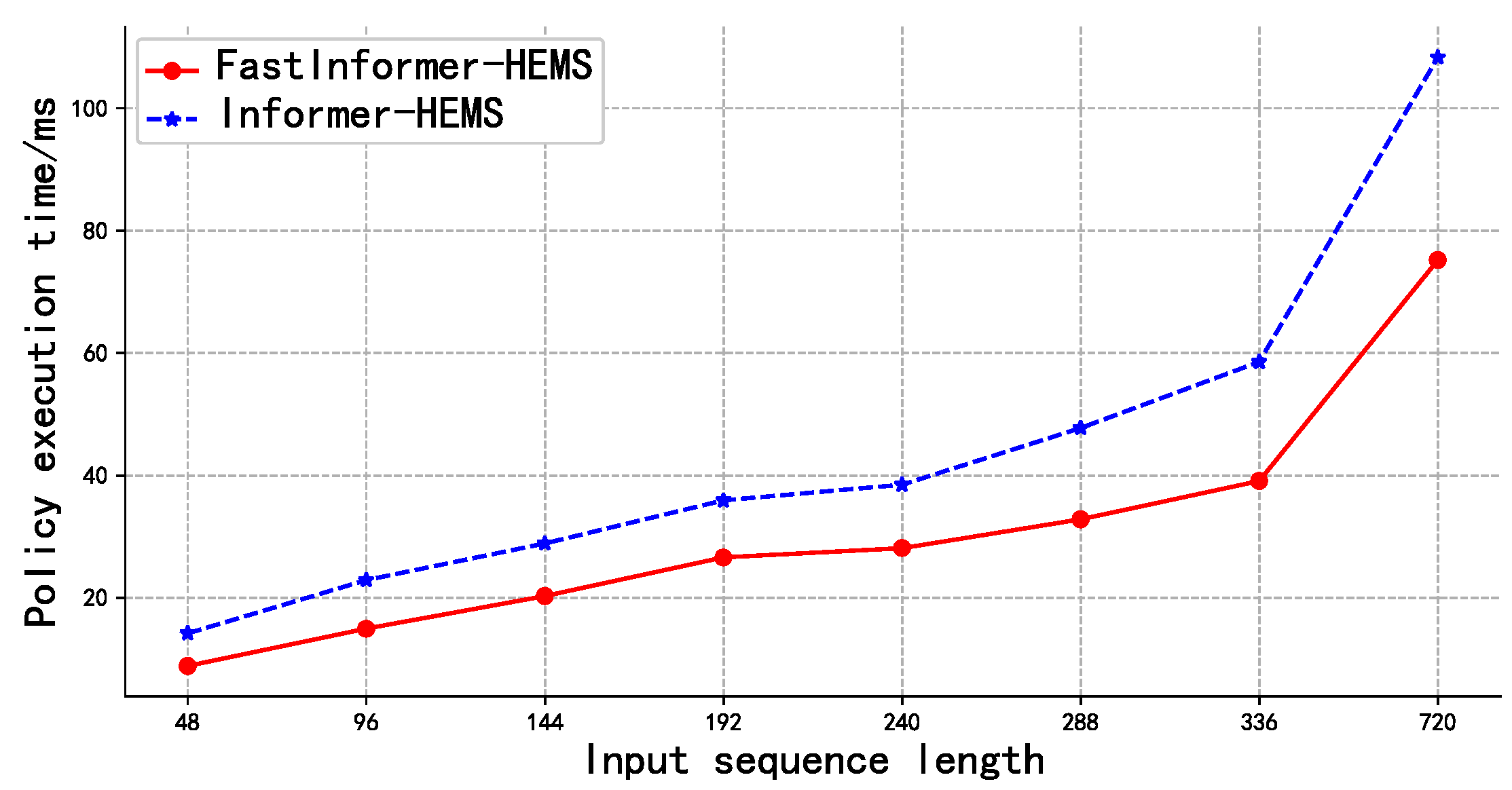
Although the execution time of the Informer-HEMS and the FastInformer-HEMS are similar, the FastInformer-HEMS performs better with the increase in input sequence length, as shown in Figure 13.
It can be seen from Figure 13 that the execution speed of the FastInformer-HEMS is faster than that of the Informer-HEMS. With the increase in the length of the input sequence, the gap between the two policies becomes larger and larger.
Compared to the Informer-HEMS, the cost of the FastInformer-HEMS over several days, as shown in Section 4.4.2, is 3% higher, but the execution time is reduced by 34.8%, which is more suitable for deployment on the end-user side with limited computing resources.
5. Conclusions
This paper proposes a lightweight optimization algorithm for a home energy management system, the FastInformer-HEMS, which introduces the E-Attn attention mechanism and uses global average pooling to extract attention features. It realizes the battery energy level’s multi-step prediction while effectively reducing the computational complexity of Informer. At the same time, SCM is introduced as an alternative security policy for the first time to ensure that the policy is feasible. In order to verify the effectiveness of the algorithm, real family data are selected for simulation experiments in one day and multiple days of the decision-making period.
The results show that the FastInformer-HEMS has the shortest execution time. Additionally, the existing MILP algorithm is not suitable for execution on the end-user side for its high computational complexity. The LSTM-HEMS can effectively solve the problem of the high computational complexity of MILP, but its optimization outcome is not high due to the accumulation of prediction errors. Compared to the existing LSTM-HEMS policy, the proposed policy can further reduce the power consumption cost of the system. Compared with the Informer-HEMS, the proposed policy can achieve a better balance between computational complexity and the optimization outcome.
Future work will focus on the classification of user power consumption patterns and the improvement of the model structure to further improve the quality of solutions.
Author Contributions
Conceptualization, X.C. and D.N.; methodology, X.C.; software, X.C.; validation, X.C.; formal analysis, X.C.; investigation, X.C.; resources, X.C.; data curation, X.C.; writing—original draft preparation, X.C.; writing—review and editing, X.C. and D.N.; visualization, X.C.; supervision, D.N.; project administration, D.N.; funding acquisition, D.N. All authors have read and agreed to the published version of the manuscript.
Funding
This research received no external funding.
Data Availability Statement
The data used in this article can be found in Smart-Grid Smart-City Customer Trial Data—Dataset—data.gov.au.
Conflicts of Interest
The authors declare no conflict of interest.
References
- Paridari, K.; Nordstrom, L.; Sandels, C. Aggregator strategy for planning demand response resources under un-certainty based on load flexibility modeling. In Proceedings of the 2017 IEEE International Conference on Smart Grid Communications, Dresden, Germany, 23–27 October 2017; pp. 338–343. [Google Scholar]
- Kwac, J.; Flora, J.; Rajagopal, R. Household energy consumption segmentation using hourly data. IEEE Trans. Smart Grid 2014, 5, 420–430. [Google Scholar] [CrossRef]
- Azuatalam, D.; Paridari, K.; Ma, Y.; Förstl, M.; Chapman, A.C.; Verbič, G. Energy management of small-scale PV-battery systems: A systematic review considering practical implementation, computational requirements, quality of input data and battery degradation. Renew. Sustain. Energy Rev. 2019, 112, 555–570. [Google Scholar] [CrossRef]
- Bouakkaz, A.; Mena, A.J.G.; Haddad, S.; Ferrari, M.L. Efficient energy scheduling considering cost reduction and energy saving in hybrid energy system with energy storage. J. Energy Storage 2021, 33, 101887. [Google Scholar] [CrossRef]
- Ahmad, A.; Khan, A.; Javaid, N.; Hussain, H.M.; Abdul, W.; Almogren, A.; Alamri, A.; Niaz, I.A. An optimized home energy management system with integrated renewable energy and storage resources. Energies 2017, 10, 549. [Google Scholar] [CrossRef]
- Azuatalam, D.; Verbic, G.; Chapman, A. Impacts of net-work tariffs on distribution network power flows. In Proceedings of the 2017 Australasian Universities Power Engineering Conference (AUPEC), Melbourne, VIC, Australia, 19–22 November 2017; pp. 1–6. [Google Scholar]
- Keerthisinghe, C.; Verbič, G.; Chapman, A.C. A Fast Technique for Smart Home Management: ADP With Temporal Difference Learning. IEEE Trans. Smart Grid 2018, 9, 3291–3303. [Google Scholar] [CrossRef]
- Zhao, Z.; Keerthisinghe, C. A Fast and Optimal Smart Home Energy Management System: State-Space Approximate Dynamic Programming. IEEE Access 2020, 8, 184151–184159. [Google Scholar] [CrossRef]
- Keerthisinghe, C.; Verbič, G.; Chapman, A.C. Addressing the stochastic nature of energy management in smart homes. In Proceedings of the 2014 Power Systems Computation Conference, Wroclaw, Poland, 18–22 August 2014; pp. 1–7. [Google Scholar]
- Xu, X.; Jia, Y.; Xu, Y.; Xu, Z.; Chai, S.; Lai, C.S. A Multi-Agent Reinforcement Learning-Based Data-Driven Method for Home Energy Management. IEEE Trans. Smart Grid 2020, 11, 3201–3211. [Google Scholar] [CrossRef]
- Mnih, V.; Kavukcuoglu, K.; Silver, D.; Rusu, A.A.; Veness, J.; Bellemare, M.G.; Graves, A.; Riedmiller, M.; Fidjeland, A.K.; Ostrovski, G.; et al. Human-level control through deep reinforcement learning. Nature 2015, 518, 529–533. [Google Scholar] [CrossRef] [PubMed]
- Yu, L.; Xie, W.; Xie, D.; Zou, Y.; Zhang, D.; Sun, Z.; Zhang, L.; Zhang, Y.; Jiang, T. Deep reinforcement learning for smart home energy management. IEEE Internet Things J. 2019, 7, 2751–2762. [Google Scholar] [CrossRef]
- Chen, S.; Wang, M.; Song, W.; Yang, Y.; Li, Y.; Fu, M. Stabilization approaches for reinforcement learning-based end-to-end autonomous driving. IEEE Trans. Veh. Technol. 2020, 69, 4740–4750. [Google Scholar] [CrossRef]
- Dinh, H.T.; Lee, K.-H.; Kim, D. Supervised-learning-based hour-ahead demand response for a behavior-based home energy management system approximating MILP optimization. Appl. Energy 2022, 321, 119382. [Google Scholar] [CrossRef]
- Kim, Y.J. A supervised-learning-based strategy for optimal demand response of an hvac system in a multi-zone office building. IEEE Trans. Smart Grid 2020, 11, 4212–4226. [Google Scholar] [CrossRef]
- Dinh, H.T.; Kim, D. Milp-based imitation learning for hvac control. IEEE Internet Things J. 2021, 9, 6107–6120. [Google Scholar] [CrossRef]
- Gao, S.; Xiang, C.; Yu, M.; Tan, K.T.; Lee, T.H. Online optimal power scheduling of a microgrid via imitation learning. IEEE Trans. Smart Grid 2021, 13, 861–876. [Google Scholar] [CrossRef]
- Paridari, K.; Azuatalam, D.; Chapman, A.C.; Verbič, G.; Nordström, L. A plug-and-play home energy management algorithm using optimization and machine learning techniques. In Proceedings of the 2018 IEEE International Conference on Communications, Control, and Computing Technologies for Smart Grids, Aalborg, Denmark, 29 October–1 November 2018; pp. 1–6. [Google Scholar]
- Vaswani, A.; Shazeer, N.; Parmar, N.; Uszkoreit, J.; Jones, L.; Gomez, A.N.; Kaiser, L.; Polosukhin, I. Attention is all you need. In Proceedings of the 31st International Conference on Neural Information Processing Systems (NIPS’17), Long Beach, CA, USA, 4–9 December 2017; Curran Associates Inc.: Red Hook, NY, USA, 2017; pp. 6000–6010. [Google Scholar]
- Zhou, H.; Zhang, S.; Peng, J.; Zhang, S.; Li, J.; Xiong, H.; Zhang, W. Informer: Beyond Efficient Transformer for Long Sequence Time-Series Forecasting. In Proceedings of the Thirty-Fifth AAAI Conference on Artificial Intelligence (AAAI-21), Virtual, 2–9 February 2021. [Google Scholar]
- Guo, M.-H.; Liu, Z.-N.; Mu, T.-J.; Hu, S.-M. Beyond Self-Attention: External Attention Using Two Linear Layers for Visual Tasks. IEEE Trans. Pattern Anal. Mach. Intell. 2022, 45, 5436–5447. [Google Scholar] [CrossRef] [PubMed]
- Ausgrid, Smart-Grid Smart-City Customer Trial Data, Online, 2016, data.gov. Available online: https://data.gov.au/dataset/smart-grid-smart-city-customer-trial-data (accessed on 10 March 2023).
- Xavier, L.S.; De Sousa, C.V.; Pereira, H.A.; Mendes, V.F. Design and performance comparisons of power converters for battery energy storage systems. Int. J. Circ. Theor. Appl. 2023; in press. [Google Scholar] [CrossRef]
Figure 1.
System architecture in a smart home.

Figure 2.
Main types of multi-horizon forecasting models. (a) Iterative one-step; (b) multi-step.

Figure 3.
Framework of FastInformer-HEMS.

Figure 4.
Alternate safe policy.

Figure 5.
Policy generation process.

Figure 6.
FastInformer model.

Figure 7.
Attention module. (a) ProbSparse attention; (b) E-Attn attention.

Figure 8.
Information of electricity price.

Figure 9.
Prediction of battery’s energy level in scenario one.

Figure 10.
Prediction of battery’s energy level in scenario two.

Figure 11.
Optimization results of algorithms in scenario one. (a) MILP; (b) LSTM-HEMS; (c) Informer-HEMS; (d) FastInformer-HEMS.
Figure 11.
Optimization results of algorithms in scenario one. (a) MILP; (b) LSTM-HEMS; (c) Informer-HEMS; (d) FastInformer-HEMS.

Figure 12.
Optimization results of algorithms in scenario two. (a) MILP; (b) LSTM-HEMS; (c) Informer-HEMS; (d) FastInformer-HEMS.
Figure 12.
Optimization results of algorithms in scenario two. (a) MILP; (b) LSTM-HEMS; (c) Informer-HEMS; (d) FastInformer-HEMS.


Figure 13.
Policy execution time comparison.


Table 1.
Battery Specifications.
| Variable | Value |
|---|---|
| Battery capacity (kWh) | 14.0 |
| Depth of discharge (kWh) | 13.5 |
| Maximum charging power (kW) | 5.0 |
| Efficiency | 90% |
Table 2.
Search space of model hyperparameter.
| Hyperparameter | Space |
|---|---|
| Input length of encoder | [12-336] |
| Label length of decoder | [4-168] |
| Output length of decoder | [1-96] |
| Batch size | [1-64] |
| Attention heads | [4,8,16] |
Table 3.
Instance information of typical scenarios.
| Typical Scenarios | Electricity Demand (kWh) | PV Generation (kWh) |
|---|---|---|
| Scenario 1 | 21.770 | 31.739 |
| Scenario 2 | 19.699 | 9.136 |
Table 4.
Costs of policies over a day.
| Policies | Cost in Scenario 1 ($) | Cost in Scenario 2 ($) |
|---|---|---|
| Benchmark (no PV-battery) | 6.662 (100%) | 9.660 (100%) |
| MILP | 2.280 (34.2%) | 5.000 (51.8%) |
| LSTM-HEMS | 3.831 (57.5%) | 6.564 (68.0%) |
| Informer-HEMS | 2.650 (39.8%) | 5.650 (58.5%) |
| FastInformer-HEMS | 3.014 (45.2%) | 5.935 (61.4%) |
Table 5.
Costs of policies over several days.
| Policies | Cost ($/Week) | Cost ($/Month) | Cost ($/4 months) |
|---|---|---|---|
| Benchmark (no PV-battery) | 56.798 (100%) | 248.431 (100%) | 1085.108 (100%) |
| MILP | 24.660 (43.4%) | 114.096 (45.9%) | 554.285 (51.1%) |
| LSTM-HEMS | 35.113 (61.8%) | 155.766 (62.7%) | 157.505 (63.4%) |
| Informer-HEMS | 30.554 (53.8%) | 141.109 (56.8%) | 638.044 (58.8%) |
| FastInformer-HEMS | 31.543 (55.5%) | 144.338 (58.1%) | 645.639 (59.5%) |
Table 6.
Execution time of policies over a day.
| Policies | Time (s) |
|---|---|
| MILP | 10.740 |
| LSTM-HEMS | 0.204 |
| Informer-HEMS | 0.023 |
| FastInformer-HEMS | 0.015 |
Disclaimer/Publisher’s Note: The statements, opinions and data contained in all publications are solely those of the individual author(s) and contributor(s) and not of MDPI and/or the editor(s). MDPI and/or the editor(s) disclaim responsibility for any injury to people or property resulting from any ideas, methods, instructions or products referred to in the content. |
© 2023 by the authors. Licensee MDPI, Basel, Switzerland. This article is an open access article distributed under the terms and conditions of the Creative Commons Attribution (CC BY) license (https://creativecommons.org/licenses/by/4.0/).
Share and Cite
MDPI and ACS Style
Chen, X.; Ning, D. FastInformer-HEMS: A Lightweight Optimization Algorithm for Home Energy Management Systems. Energies 2023, 16, 3897. https://doi.org/10.3390/en16093897
AMA Style
Chen X, Ning D. FastInformer-HEMS: A Lightweight Optimization Algorithm for Home Energy Management Systems. Energies. 2023; 16(9):3897. https://doi.org/10.3390/en16093897
Chicago/Turabian StyleChen, Xihui, and Dejun Ning. 2023. "FastInformer-HEMS: A Lightweight Optimization Algorithm for Home Energy Management Systems" Energies 16, no. 9: 3897. https://doi.org/10.3390/en16093897
Note that from the first issue of 2016, this journal uses article numbers instead of page numbers. See further details here.