
Steady-State Load Flow Model of DFIG Wind Turbine Based on Generator Power Loss Calculation

Department of Electrical Engineering, Tanjungpura University, Pontianak 78124, Indonesia
*
Author to whom correspondence should be addressed.
Energies 2023, 16(9), 3640; https://doi.org/10.3390/en16093640
Submission received: 16 March 2023
/
Revised: 6 April 2023
/
Accepted: 12 April 2023
/
Published: 24 April 2023
(This article belongs to the Special Issue Advances in Power System Analysis and Control)
Abstract
:Penetration of wind power plants (WPPs) in the electric power system will complicate the system load flow analysis. Consequently, the traditional load flow algorithm can no longer be used to find the solution to the load flow problem of such a system. This paper proposes a doubly fed induction generator (DFIG)-based WPP model for a load flow analysis of the electric power system. The proposed model is derived based on the power formulations of the WPP—namely, DFIG power, DFIG power loss, and WPP power output formulas. The model can be applied to various DFIG power factor operating modes. In the present paper, applications of the proposed methods in two representative electric power systems (i.e., IEEE 14-bus and 30-bus systems) have been investigated. The investigation results verify the proposed method’s capability to solve the load flow problem of the system embedded with DFIG-based variable-speed WPPs.
1. Introduction
Information about the steady-state performances of an electric power system is usually obtained from load flow analysis. Quantities such as system voltages, generator powers, line power flows, and line losses are generally available as the output of the analysis. Based on the load flow results, an assessment or evaluation of the power system performance can then be carried out. If some values of the electrical quantities are outside the limits, corrective action needs to be taken to bring the quantities back to their allowable limits.
It has been well acknowledged that penetration of WPPs in the electric power system will complicate the system load flow analysis. Consequently, the traditional load flow algorithm can no longer be used to find the solution to the load flow problem of such a system. Several techniques for solving the load flow problem of power systems embedded with WPPs have been proposed, and some of the current methods are reported in [1,2,3,4,5,6,7,8,9,10,11,12,13]. In [1,2,3], three-node models of fixed-speed WPPs were proposed. By using these models, conventional load flow programs can be employed in the analysis. In [4], the models for representing asynchronous generator-based fixed-speed WPPs have been proposed. The models in [4] were developed based on the formulas that calculate the electric powers exchanged between the WPPs and the power grid. A fixed-speed WPP model for distribution load flow analysis has been proposed in [5]. In [5], the WPP model was formulated in the form of WPP output power.
In [6,7], three-phase models of DFIG-based variable-speed WPPs have been proposed. In [6], the model was derived in the form of DFIG output power and expressed in terms of bus voltage and wind speed. In [7], the DFIG model was formed using the sequence components theory. A technique to integrate DFIG-based WPPs in load flow analysis was discussed in [8]. The equivalent circuit of the induction generator has been used in the proposed approach [8]. In [9], a load flow model of the DFIG under power control has been proposed. Limitations of the DFIG and the power system were simultaneously solved to achieve the desired output. The DFIG model in [10] was based on an induction generator equivalent circuit and also took into consideration the voltage-dependent reactive power limits associated with the DFIG. References [11,12,13] proposed various models of DFIGs for load flow analysis. Derivation of the models has been carried out based on the WPP power formulas. However, in [11], the DFIG power factor was assumed to be unity. In [12], a DFIG steady-state model in voltage control mode of operation was proposed. In the method, DFIG voltage can be regulated by allowing the power factor to change. A simple load flow model of the DFIG was proposed in [13]. The model can be used for DFIGs operating in power factor control mode. Three DFIG power factor operation modes (i.e., unity, lagging, and leading) were considered in [13].
This paper presents a model of a DFIG-based variable-speed WPP for a load flow analysis of an electric power system. The proposed model is derived based on the power formulations of the WPP—namely, DFIG power, DFIG power loss, and WPP power output formulas. The model proposed in this paper also serves as an alternative to the model discussed in [13]. It, therefore, retains the important features as follows: (i) the model can be applied to all three power factor (PF) modes of operation—namely, UPF (unity PF), LePF (leading PF), and LaPF (lagging PF), and (ii) both DFIG conditions (i.e., sub-synchronous and super-synchronous) can be modeled using the same equations. Moreover, as the model in this paper is derived based on induction generator power losses calculation, the generator power losses are readily available as the output of the proposed method.
More results are also included in the present paper to verify the method further. In addition to the IEEE 14-bus power network, a more complex electric power network (i.e., IEEE 30-bus system) is also used and investigated in the case study. Based on the investigation results, verification of the proposed method is obtained. The rest of the paper is organized as follows. Section 2 briefly discusses the basic configuration and equivalent circuit of the DFIG. The proposed model is also presented in this section. The application of the method in finding the solution to the power system load flow is given in Section 3. Section 4 points out some important conclusions of the present work.
2. DFIG-Based Wind Turbine
2.1. DFIG Configuration and Equivalent Circuit
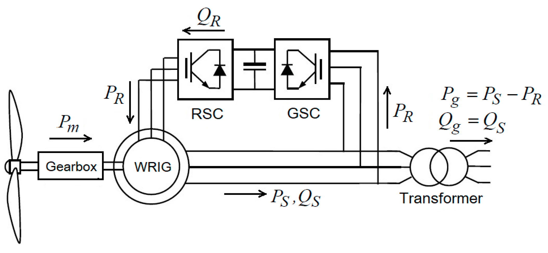
The basic configuration of the DFIG is presented in Figure 1 [11,12,13,14,15,16,17,18]. It can be seen from Figure 1 that the main components of the DFIG system include the wind turbine, gearbox, WRIG (wound rotor induction generator), and power electronic converter (PEC). The PEC, which consists of the RSC (rotor side converter), DC link, and GSC (grid side converter), has the function of regulating WRIG rotor reactive power. In Figure 1, Pm is turbine power, PS and QS are WRIG stator powers, Pg and Qg are DFIG output powers, and PR and QR are WRIG rotor powers.
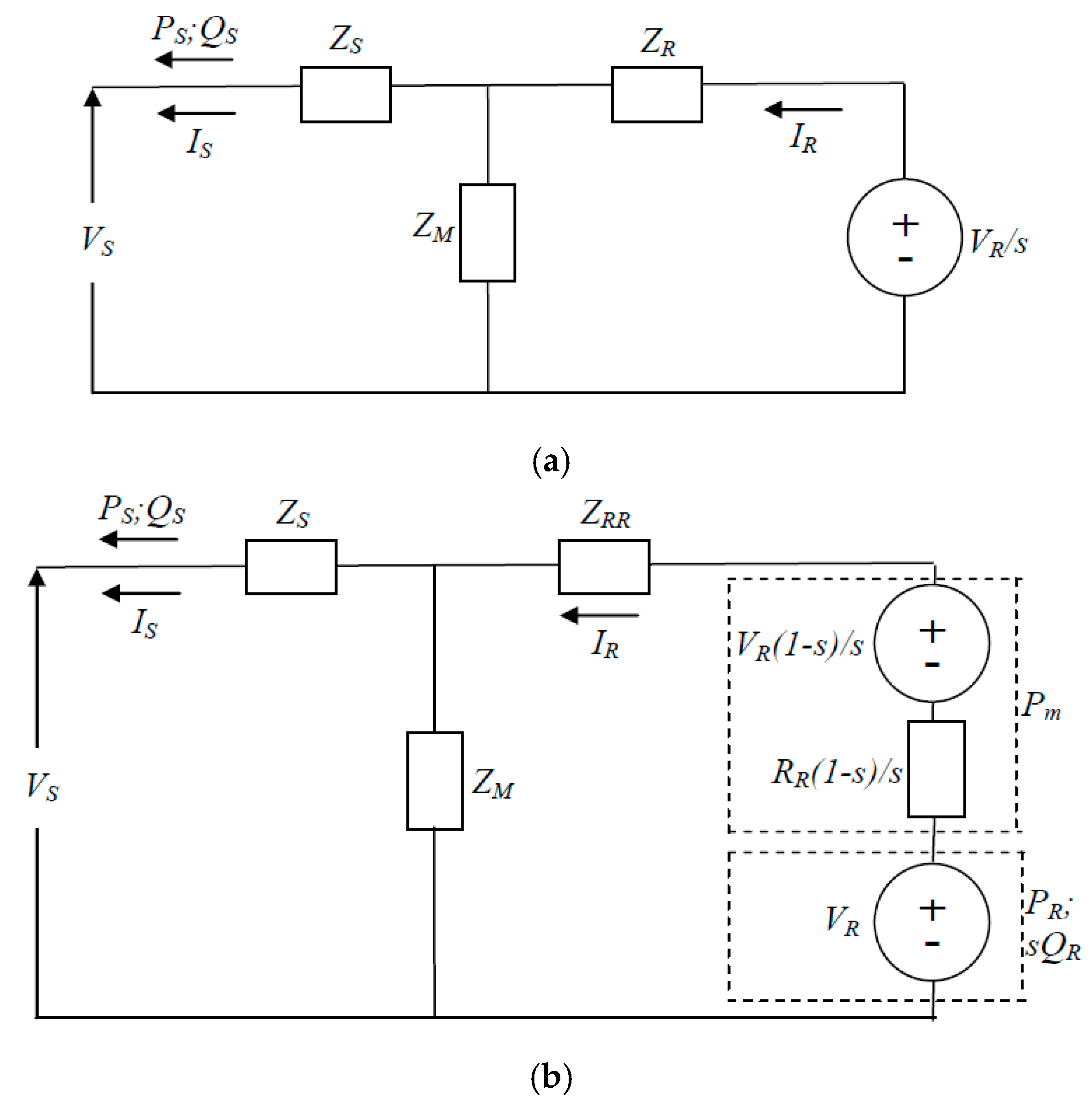
Figure 2 shows steady-state equivalent circuits of the DFIG [11,12,13,14,15,16,17,18]. In Figure 2, VS and IS are stator voltage and current, VR and IR are rotor voltage and current, and s is WRIG slip. The impedances (i.e., ZS, ZR, ZRR, and ZM) in Figure 2 are determined based on the induction generator resistance, reactance, and slip as follows:
where RS and XS are stator resistance and reactance, RR and XR are rotor resistance and reactance, and Rc and Xm are core circuit resistance and reactance of WRIG.
DFIG-based wind turbines can be operated in power factor control mode. In the power factor control mode of operation, the DFIG is set to regulate the power factor. Three power factors (i.e., leading, lagging, and unity) are usually adopted in the DFIG operation. The DFIG can deliver reactive power to the power system or grid in LePF operation. In this mode of operation, the DFIG can be employed to support the system’s reactive power demand and improve the voltage profile. On the other hand, in LaPF operation, the DFIG absorbs reactive power from the grid. This reactive power (together with the reactive power produced by the DFIG rotor) is used for induction generator magnetization. In UPF operation, no reactive power is delivered or absorbed to or from the grid. All reactive power needed for magnetization comes from the DFIG rotor.
2.2. DFIG Power and WRIG Loss Formulas
By looking at Figure 1, the WPP active and reactive power outputs are:
and
where ϕ is the DFIG power factor angle.
On using (4) and (5) in (2), the WPP active power output becomes:
In addition to the above power formulas, power loss in the WRIG will also be used in deriving the proposed DFIG steady-state load flow model. Based on Figure 2b, WRIG power loss is:
Rearranging (7), WRIG power loss can be formulated as:
2.3. DFIG Steady-State Load Flow Model
Power loss in the DFIG system is the difference between power input and power output of the DFIG. Since the active and reactive power inputs are Pm and QR, and the active and reactive power outputs are Pg and Qg, then the following relationships are valid:
and
It is to be noted that power losses in the DFIG power electronic converter are very small compared to those in the WRIG. Therefore, in (9) and (10), they have been neglected. Equations (3) and (6) can be combined to obtain a more compact formulation as follows:
where (4) has also been used in forming the combination. In the same way, combining (9) and (10) results in:
Based on (11) and (12), the steady-state model of a WPP that uses a DFIG as its primary energy converter can be formulated as:
In the load flow study of a system embedded with DFIG-based WPPs, (13) is used in conjunction with the following power system nodal equation [13]:
In (14), SG and SL are power generation and power demand, V is nodal voltage, Y is nodal admittance matrix, and n is the total number of power system nodes. Table 1 gives the equations to be solved and quantities to be calculated in the load flow analysis. It is to be noted that VS = |VS|∟δS in (13) is also the voltage at the WPP bus (i.e., V = |V|∟δ). Furthermore, the stator and rotor currents in (8) and (13) can be expressed in terms of stator and rotor voltages as follows [11]:
where
3. Case Study
3.1. WPP Data
The WPP used in the study is assumed to consist of 100 identical wind turbine generator (WTG) units. Data of the WTG and generator slip and turbine power values used in the case study can be found in [13]. To simplify the calculation in load flow analysis, the WPP is aggregated into a single machine equivalent. Parameters of the WPP single machine equivalent can also be found in [13].
3.2. Test Systems
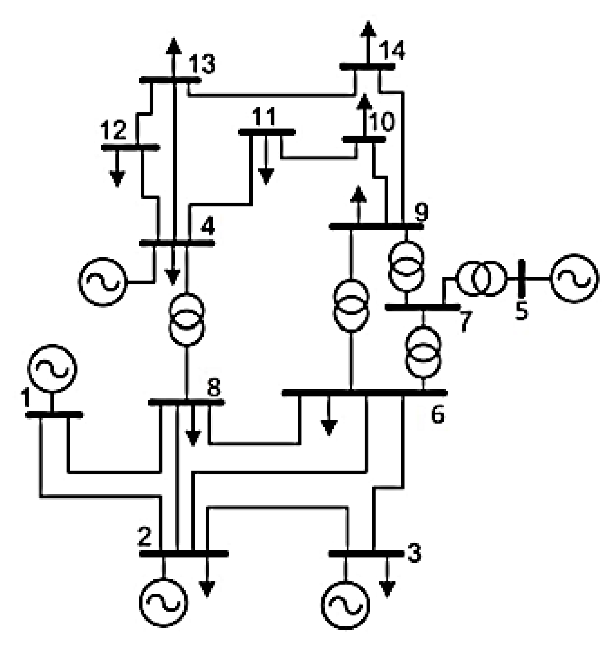
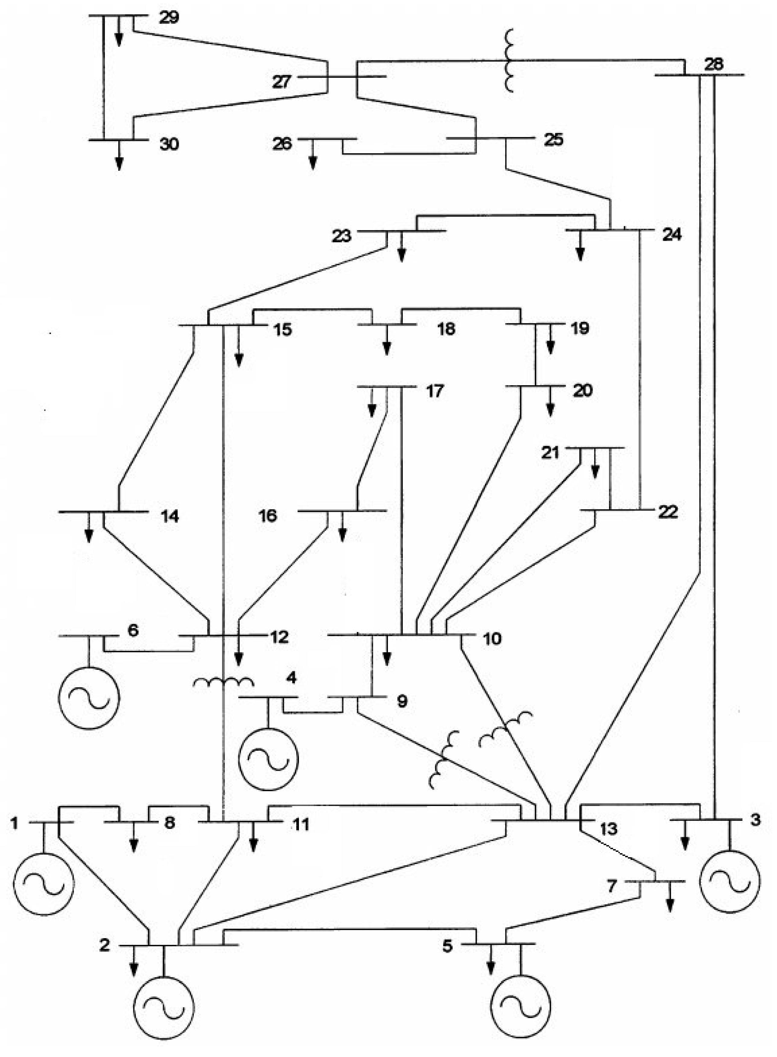
Two representative power systems (i.e., IEEE 14-bus and 30-bus systems) adapted from [19] will be used to test the method proposed in Section 2. Single-line diagrams of the systems are displayed in Figure 3 and Figure 4. For the IEEE 14-bus, the line and load data can be found in [13]. On the other hand, details of the line and load data for the 30-bus system are given in Table 2 and Table 3. The total three-phase loads for both test systems and locations of the WPP (i.e., WPP point of connection) are summarized in Table 4. In both systems, the WPP is connected to the power system via a step-up transformer. The transformer impedance is assumed to be j0.05 pu. It is to be noted that the base for all data in pu is 100 MVA.
3.3. Results and Discussion
By using the slip and turbine power values described in Section 3.1, load flow studies for the systems in Figure 3 and Figure 4 were then conducted. The results of these studies are presented in Table 5, Table 6, Table 7, Table 8, Table 9, Table 10, Table 11, Table 12, Table 13, Table 14, Table 15 and Table 16. Some of the results are also given in graphical form (see Figure 5, Figure 6, Figure 7, Figure 8, Figure 9 and Figure 10) to make the observation easier. Three DFIG power factor (PF) modes of operation (i.e., LePF, LaPF, and UPF) have been considered and investigated in the studies. It is to be noted that the results in Table 5, Table 6, Table 7, Table 8, Table 9 and Table 10 are in exact agreement with the results in [13], which confirms the validity of the proposed model.
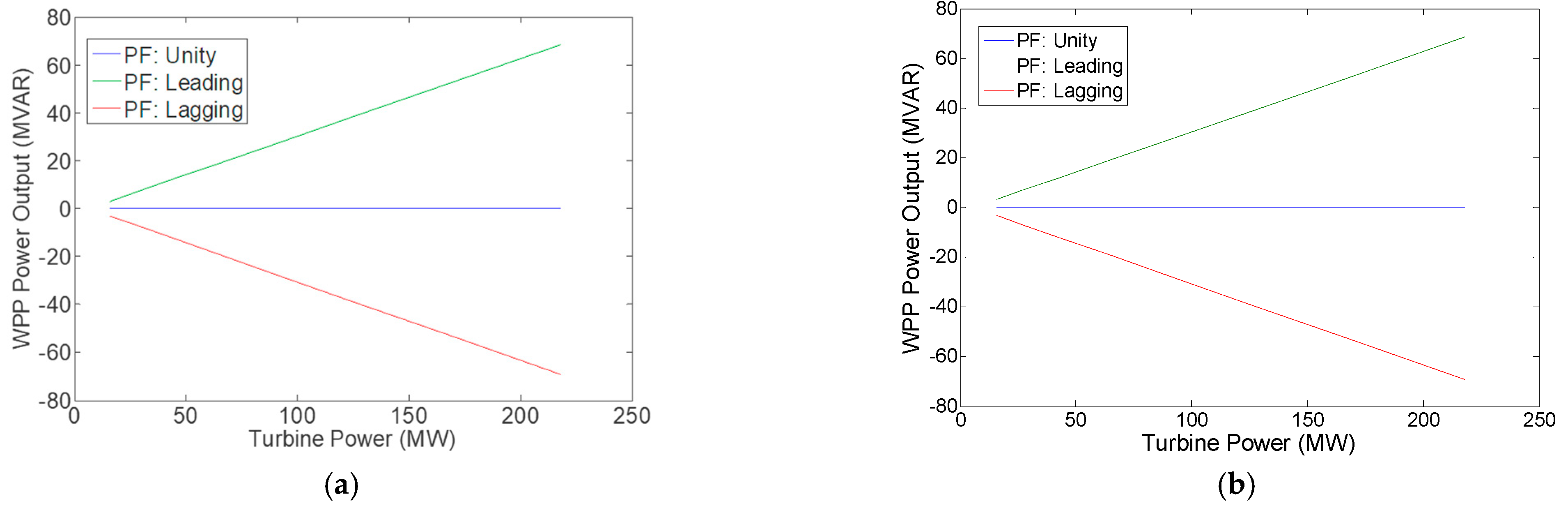
The results in Table 5 and Table 11 show that, in the UPF operating mode, the WPP reactive power output is always zero (no reactive power is delivered or absorbed by the WPP). In this mode of operation, the rotor’s reactive power is used for induction generator magnetization. In LePF operating mode (see Table 7 and Table 13), the WPP reactive power output is always positive (i.e., the WPP delivers reactive power to the power system or grid). In this operation mode, most of the reactive power produced by the rotor is used for magnetization, while the rest of the reactive power is used to support the system’s reactive power demand.
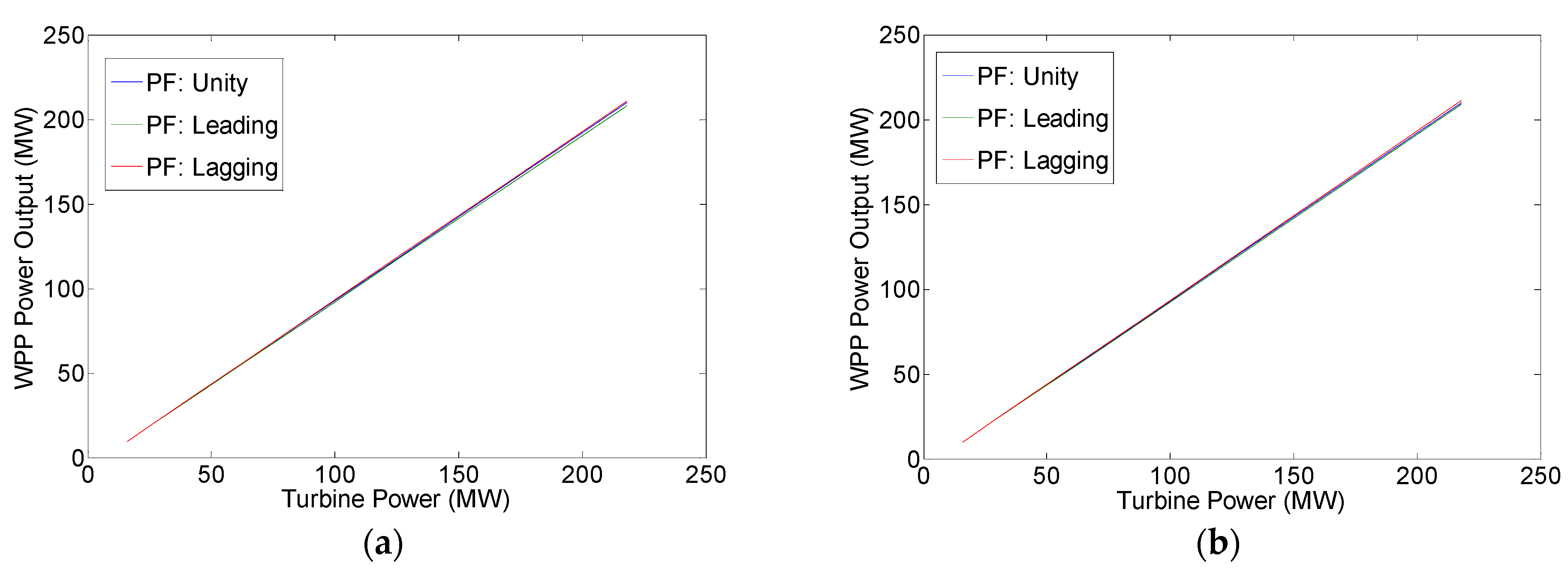
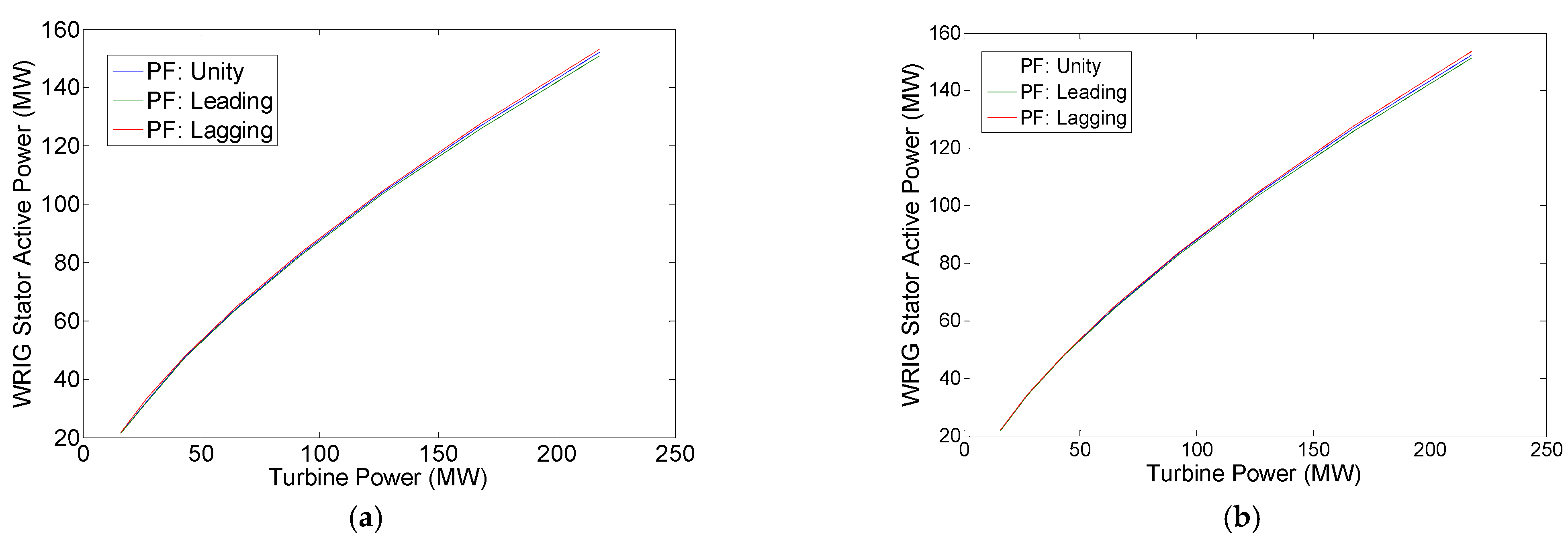
On the other hand, in LaPF operating mode (see Table 9 and Table 15), the WPP reactive power output is always negative (i.e., the WPP absorbs reactive power from the grid). In this mode of operation, the reactive power for generator magnetization comes from the DFIG rotor and power grid. It should also be noted that the WPP will always deliver active power to the grid in the above three modes of operation. Figure 5 and Figure 6 show the variations of WPP active power and WPP reactive power, respectively. The values of WRIG stator active power for the three power factor operating modes are given in Table 5, Table 7, Table 9, Table 11, Table 13 and Table 15. These WRIG stator active power variations are also presented in graphical form (see Figure 7). It can be seen that the values of the WRIG stator active power are almost not affected by the DFIG power factor.
The load flow analysis also provides the values of the rotor’s active powers (see Table 5, Table 7, Table 9, Table 11, Table 13 and Table 15). In DFIG sub-synchronous operations, the rotor’s active power is always positive (power is absorbed). On the other hand, in DFIG super-synchronous operations, the rotor’s active power is always negative (power is delivered). These rotor active powers are also almost not affected by the DFIG power factor. These results verify the validity of the proposed model to represent the DFIG in both sub-synchronous and super-synchronous conditions.
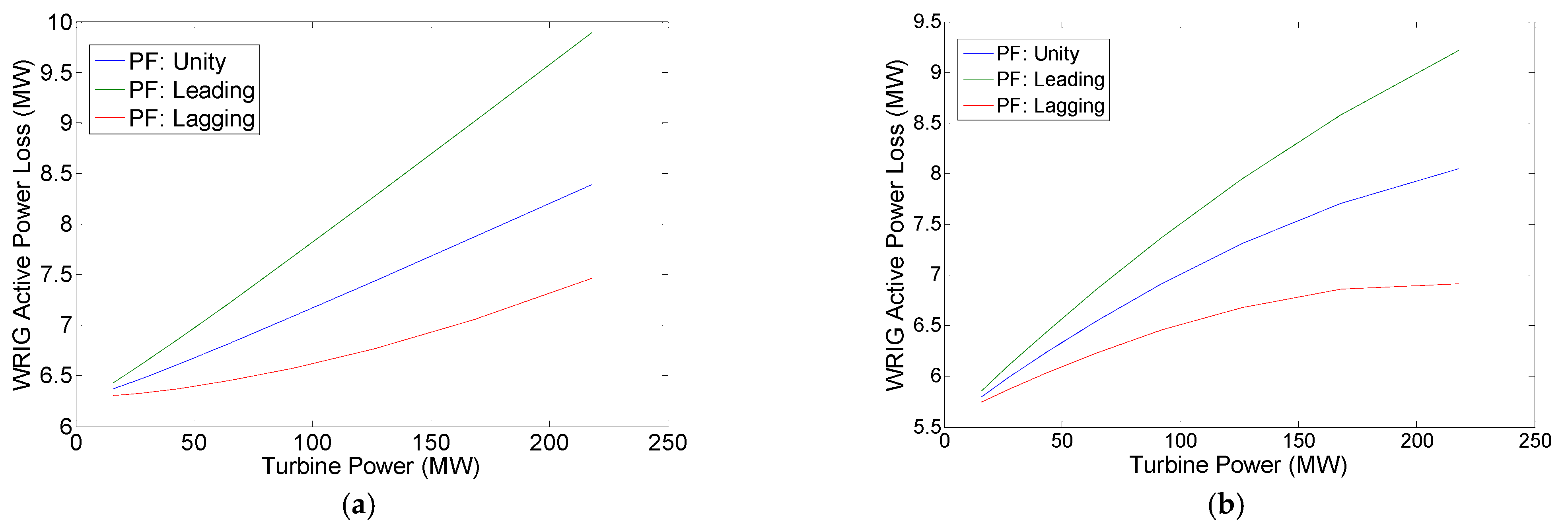
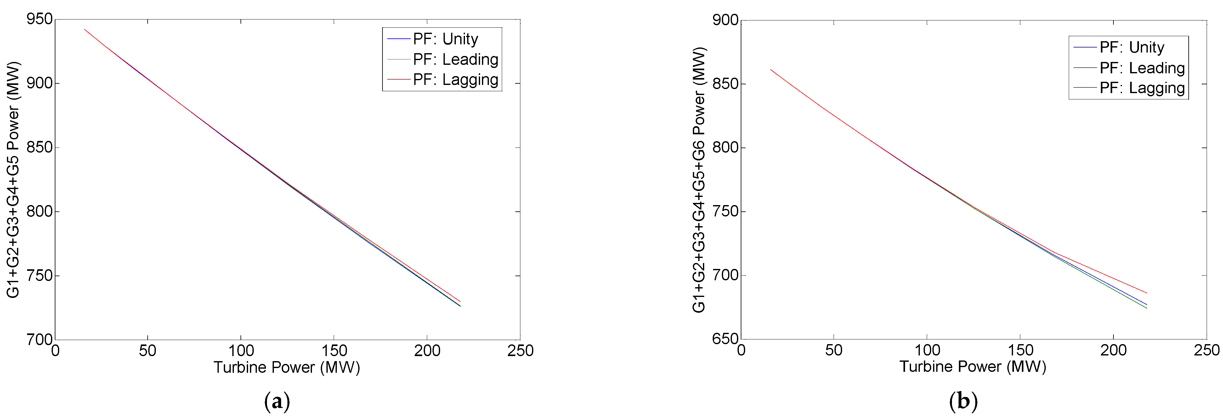
Table 5, Table 7, Table 9, Table 11, Table 13 and Table 15 show the values of WRIG power loss for the three power factor operating modes. These WRIG power losses are calculated using (8) and are readily available as the output of the proposed algorithm. It can be seen that the WRIG power loss increases when the turbine mechanical power (i.e., DFIG power output) goes up (see also Figure 8 and Figure 9). This result is expected since more current is flowing in the WRIG circuit as the DFIG power output is raised. Table 6, Table 8, Table 10, Table 12, Table 14 and Table 16 show that the conventional power plant output can be reduced as the turbine and WPP output powers are increased (see also Figure 10). It can also be observed from the load flow results that for each case of turbine power, the WPP output plus conventional power plant output is always equal to the total system load plus line losses. These results further verify the validity of the proposed method.
4. Conclusions
In this paper, a model of a DFIG-based WPP for a load flow analysis of electric power systems has been proposed. The proposed model is derived based on the power formulations of the WPP—namely, DFIG power, DFIG power loss, and WPP power output formulas. The model can be applied to various DFIG power factor operating modes, i.e., UPF, LePF, and LaPF. Both DFIG conditions (i.e., sub-synchronous and super-synchronous) can be modeled using the same equations. As the model in this paper is derived based on induction generator power losses calculation, the generator power losses are readily available as the output of the proposed method. Results of the case studies are also given in the present paper. In the case study, applications of the proposed methods on representative electric power systems have been investigated. Based on the investigation results, verification of the proposed method has been obtained. For future work, the DFIG model proposed in the present paper can be used as a reference to develop other variable-speed WPPs (SCIG-based variable-speed WPPs and PMSG-based WPPs).
Author Contributions
Conceptualization, R.G. and P.; methodology, R.G. and P.; software, R.G.; validation, R.G., P., and F.I.; formal analysis, R.K.; investigation, D.; resources, F.I.; data curation, R.K.; writing—original draft preparation, R.G.; writing—review and editing, P.; visualization, D.; supervision, F.I.; project administration, R.K.; funding acquisition, D. All authors have read and agreed to the published version of the manuscript.
Funding
This research was funded by Kemendikbud-Ristek Republik Indonesia.
Data Availability Statement
Not applicable.
Conflicts of Interest
The authors declare no conflict of interest.
References
- Haque, M.H. Evaluation of power flow solutions with fixed speed wind turbine generating systems. Energy Convers. Manag. 2014, 79, 511–518. [Google Scholar] [CrossRef]
- Haque, M.H. Incorporation of fixed speed wind turbine generators in load flow analysis of distribution systems. Int. J. Renew. Energy Technol. 2015, 6, 317–324. [Google Scholar] [CrossRef]
- Wang, J.; Huang, C.; Zobaa, A.F. Multiple-node models of asynchronous wind turbines in wind farms for load flow analysis. Electr. Power Compon. Syst. 2015, 44, 135–141. [Google Scholar] [CrossRef]
- Feijoo, A.; Villanueva, D. A PQ model for asynchronous machines based on rotor voltage calculation. IEEE Trans. Energy Convers. 2016, 31, 813–814, Correction in IEEE Trans. Energy Convers. 2016, 31, 1228. [Google Scholar] [CrossRef]
- Ozturk, O.; Balci, M.E.; Hocaoglu, M.H. A new wind turbine generating system model for balanced and unbalanced distribution systems load flow analysis. Appl. Sci. 2018, 8, 502. [Google Scholar]
- Dadhania, A.; Venkatesh, B.; Nassif, A.B.; Sood, V.K. Modeling of doubly fed induction generators for distribution system power flow analysis. Electr. Power Energy Syst. 2013, 53, 576–583. [Google Scholar] [CrossRef]
- Ju, Y.; Ge, F.; Wu, W.; Lin, Y.; Wang, J. Three-phase steady-state model of DFIG considering various rotor speeds. IEEE Access 2016, 4, 9479–9948. [Google Scholar] [CrossRef]
- Kumar, V.S.S.; Thukaram, D. Accurate modeling of doubly fed induction based wind farms in load flow analysis. Electr. Power Syst. Res. 2018, 15, 363–371. [Google Scholar]
- Li, S. Power flow modeling to doubly-fed induction generators (DFIGs) under power regulation. IEEE Trans. Power Syst. 2013, 28, 3292–3301. [Google Scholar] [CrossRef]
- Anirudh, C.V.S.; Seshadri, S.K.V. Enhanced modeling of doubly fed induction generator in load flow analysis of distribution systems. IET Renew. Power Gener. 2021, 15, 980–989. [Google Scholar]
- Gianto, R. Steady state model of DFIG-based wind power plant for load flow analysis. IET Renew. Power Gener. 2021, 15, 1724–1735. [Google Scholar] [CrossRef]
- Gianto, R. Constant voltage model of DFIG-based variable speed wind turbine for load flow analysis. Energies 2021, 14, 8549. [Google Scholar] [CrossRef]
- Gianto, R. Constant power factor model of DFIG-based wind turbine for steady state load flow analysis. Energies 2022, 15, 6077. [Google Scholar] [CrossRef]
- Anaya-Lara, O.; Jenkins, N.; Ekanayake, J.B.; Cartwright, P.; Hughes, M. Wind Energy Generation: Modelling and Control; John Wiley & Sons, Ltd.: Chichester, UK, 2009. [Google Scholar]
- Akhmatov, V. Induction Generators for Wind Power; Multi-Science Publishing Co., Ltd.: Brentwood, UK, 2007. [Google Scholar]
- Boldea, I. Variable Speed Generators; Taylor & Francis Group LLC.: Roca Baton, FL, USA, 2005. [Google Scholar]
- Fox, B.; Flynn, B.; Bryans, L.; Jenkins, J. Wind Power Integration: Connection and System Operational Aspects; The Institution of Engineering and Technology: Stevenage Herts, UK, 2007. [Google Scholar]
- Patel, M.R. Wind and Solar Power Systems; CRC Press LLC.: Boca Raton, FL, USA, 1999. [Google Scholar]
- Pai, M.A. Computer Techniques in Power System Analysis; Tata McGraw-Hill Publishing Co., Ltd.: New Delhi, India, 1984. [Google Scholar]
Figure 1.
DFIG configuration.

Figure 2.
DFIG equivalent circuits. (a) Original; (b) Modified.

Figure 3.
IEEE 14-bus system.

Figure 4.
IEEE 30-bus system.

Figure 5.
WPP active power. (a) IEEE 14-bus; (b) IEEE 30-bus.

Figure 6.
WPP reactive power. (a) IEEE 14-bus; (b) IEEE 30-bus.

Figure 7.
WRIG stator active power. (a) IEEE 14-bus; (b) IEEE 30-bus.

Figure 8.
WRIG active power loss. (a) IEEE 14-bus; (b) IEEE 30-bus.

Figure 9.
WRIG reactive power loss. (a) IEEE 14-bus; (b) IEEE 30-bus.

Figure 10.
Total active power output of conventional generators. (a) IEEE 14-bus; (b) IEEE 30-bus.


Table 1.
Equation and quantity.
| Bus | Equation(s) | Knowns | Unknowns |
|---|---|---|---|
| Slack | (14) | |V| and δ = 0° | PG and QG |
| PV | (14) | PG and |V| | δ and QG |
| PQ | (14) | PG = QG = 0 | |V| and δ |
| WPP | (13) and (14) | ϕ, s, and Pm | |V| = |VS|, δ = δS, PG = Pg, QR, Re(VR) and Im(VR) |
Table 2.
Line data of IEEE 30-bus system (in pu).
| Line | Sending Bus | Receiving Bus | Series Impedance |
|---|---|---|---|
| 1 | 1 | 2 | 0.0192 + j0.0575 |
| 2 | 1 | 8 | 0.0452 + j0.1852 |
| 3 | 2 | 11 | 0.0570 + j0.1737 |
| 4 | 8 | 11 | 0.0132 + j0.0379 |
| 5 | 2 | 5 | 0.0472 + j0.1983 |
| 6 | 2 | 13 | 0.0581 + j0.1763 |
| 7 | 11 | 13 | 0.0119 + j0.0414 |
| 8 | 5 | 7 | 0.0460 + j0.1160 |
| 9 | 7 | 13 | 0.0267 + j0.0820 |
| 10 | 3 | 13 | 0.0120 + j0.0420 |
| 11 | 9 | 13 | j0.2080 |
| 12 | 10 | 13 | j0.5560 |
| 13 | 4 | 9 | j0.2080 |
| 14 | 9 | 10 | j0.1100 |
| 15 | 11 | 12 | j0.2560 |
| 16 | 6 | 12 | j0.1400 |
| 17 | 12 | 14 | 0.1231 + j0.2559 |
| 18 | 12 | 15 | 0.0662 + j0.1304 |
| 19 | 12 | 16 | 0.0945 + j0.1987 |
| 20 | 14 | 15 | 0.2210 + j0.1997 |
| 21 | 16 | 17 | 0.0824 + j0.1932 |
| 22 | 15 | 18 | 0.1073 + j0.2185 |
| 23 | 18 | 19 | 0.0639 + j0.1292 |
| 24 | 19 | 20 | 0.0340 + j0.0680 |
| 25 | 10 | 20 | 0.0936 + j0.2090 |
| 26 | 10 | 17 | 0.0324 + j0.0845 |
| 27 | 10 | 21 | 0.0348 + j0.0749 |
| 28 | 10 | 22 | 0.0727 + j0.1499 |
| 29 | 21 | 22 | 0.0116 + j0.0236 |
| 30 | 15 | 23 | 0.1000 + j0.2020 |
| 31 | 22 | 24 | 0.1150 + j0.1790 |
| 32 | 23 | 24 | 0.1320 + j0.2700 |
| 33 | 24 | 25 | 0.1885 + j0.3292 |
| 34 | 25 | 26 | 0.2544 + j0.3800 |
| 35 | 25 | 27 | 0.1093 + j0.2087 |
| 36 | 27 | 28 | j0.3960 |
| 37 | 27 | 29 | 0.2198 + j0.4153 |
| 38 | 27 | 30 | 0.3202 + j0.6027 |
| 39 | 29 | 30 | 0.2399 + j0.4533 |
| 40 | 3 | 28 | 0.0636 + j0.2000 |
| 41 | 13 | 28 | 0.0169 + j0.0599 |
Table 3.
Bus data of IEEE 30-bus system (in pu).
| Bus | |V| | δ | Generation | Load | Note |
|---|---|---|---|---|---|
| 1 | 1.0500 | 0 | - | 0 | Slack |
| 2 | 1.0338 | - | 0.5756 + j- | 0.217 + j0.127 | PV |
| 3 | 1.0230 | - | 0.3500 + j- | 0.300 + j0.300 | PV |
| 4 | 1.0913 | - | 0.1793 + j- | 0 | PV |
| 5 | 1.0058 | - | 0.2456 + j- | 0.942 + j0.190 | PV |
| 6 | 1.0883 | - | 0.1691 + j- | 0 | PV |
| 7 | - | - | 0 | 0.228 + j0.109 | PQ |
| 8 | - | - | 0 | 0.024 + j0.012 | PQ |
| 9 | - | - | 0 | 0 | PQ |
| 10 | - | - | 0 | 0.058 + j0.020 | PQ |
| 11 | - | - | 0 | 0.076 + j0.016 | PQ |
| 12 | - | - | 0 | 0.112 + j0.075 | PQ |
| 13 | - | - | 0 | 0 | PQ |
| 14 | - | - | 0 | 0.062 + j0.016 | PQ |
| 15 | - | - | 0 | 0.082 + j0.025 | PQ |
| 16 | - | - | 0 | 0.035 + j0.018 | PQ |
| 17 | - | - | 0 | 0.090 + j0.058 | PQ |
| 18 | - | - | 0 | 0.032 + j0.009 | PQ |
| 19 | - | - | 0 | 0.095 + j0.034 | PQ |
| 20 | - | - | 0 | 0.022 + j0.007 | PQ |
| 21 | - | - | 0 | 0.175 + j0.112 | PQ |
| 22 | - | - | 0 | 0 | PQ |
| 23 | - | - | 0 | 0.032 + j0.016 | PQ |
| 24 | - | - | 0 | 0.087 + j0.067 | PQ |
| 25 | - | - | 0 | 0 | PQ |
| 26 | - | - | 0 | 0.035 + j0.023 | PQ |
| 27 | - | - | 0 | 0 | PQ |
| 28 | - | - | 0 | 0 | PQ |
| 29 | - | - | 0 | 0.024 + j0.009 | PQ |
| 30 | - | - | 0 | 0.106 + j0.019 | PQ |
Note: notation ‘-’ denotes quantities to be calculated.
Table 4.
Total system three-phase load and WPP location.
| System | Total Load (MW; MVAr) | WPP Location |
|---|---|---|
| IEEE 14-bus | 897; 243.9 | Bus 14 |
| IEEE 30-bus | 850.2; 378.6 | Bus 30 |
Table 5.
DFIG power flows and losses of 14-bus system (PF = 1.0).
| ΣPm (MW) | Pg (MW) | PS (MW) | Qg = QS (MVAR) | PR (MW) | PLOSS (MW) | QLOSS (MVAR) |
|---|---|---|---|---|---|---|
| 15.78 | 9.4127 | 21.4955 | 0 | 12.0828 | 6.3673 | 63.6728 |
| 27.27 | 20.8045 | 32.8212 | 0 | 12.0167 | 6.4655 | 64.6551 |
| 43.30 | 36.6883 | 47.9329 | 0 | 11.2446 | 6.6117 | 66.1171 |
| 64.63 | 57.8139 | 64.4185 | 0 | 6.6046 | 6.8161 | 68.1608 |
| 92.02 | 84.9318 | 83.0831 | 0 | −1.8487 | 7.0882 | 70.8821 |
| 126.23 | 118.7934 | 103.9265 | 0 | −14.8669 | 7.4366 | 74.3658 |
| 168.01 | 160.1414 | 126.9522 | 0 | −33.1892 | 7.8686 | 78.6861 |
| 218.12 | 209.7292 | 152.1444 | 0 | −57.5848 | 8.3908 | 83.9077 |
Table 6.
WPP voltages, G1 to G5 powers and losses of 14-bus system (PF = 1.0).
| ΣPm (pu) | Voltage (pu) | G1 to G5 Outputs | Line Losses | ||
|---|---|---|---|---|---|
| MW | MVAR | MW | MVAR | ||
| 15.78 | 1.0160 | 941.7797 | 479.5449 | 54.1924 | 235.6449 |
| 27.27 | 1.0196 | 928.6547 | 470.9905 | 52.4592 | 227.0905 |
| 43.30 | 1.0243 | 910.5415 | 459.8925 | 50.2298 | 215.9925 |
| 64.63 | 1.0301 | 886.7778 | 446.5797 | 47.5917 | 202.6797 |
| 92.02 | 1.0368 | 856.8002 | 431.8180 | 44.7320 | 187.9180 |
| 126.23 | 1.0440 | 820.1648 | 416.8994 | 41.9582 | 172.9994 |
| 168.01 | 1.0512 | 776.5829 | 403.7411 | 39.7243 | 159.8411 |
| 218.12 | 1.0575 | 725.9341 | 395.0049 | 38.6634 | 151.1049 |
Table 7.
DFIG power flows and losses of 14-bus system (PF = 0.95 leading).
| ΣPm (MW) | Pg (MW) | PS (MW) | Qg = QS (MVAR) | PR (MW) | PLOSS (MW) | QLOSS (MVAR) |
|---|---|---|---|---|---|---|
| 15.78 | 9.3484 | 21.4447 | 3.0727 | 12.0962 | 6.4316 | 64.3156 |
| 27.27 | 20.6617 | 32.5085 | 6.7912 | 11.8469 | 6.6083 | 66.0830 |
| 43.30 | 36.4350 | 47.7337 | 11.9756 | 11.2987 | 6.8650 | 68.6499 |
| 64.63 | 57.4122 | 64.1035 | 18.8705 | 6.6913 | 7.2178 | 72.1783 |
| 92.02 | 84.3374 | 82.6185 | 27.7203 | −1.7189 | 7.6826 | 76.8265 |
| 126.23 | 117.9556 | 103.2733 | 38.7701 | −14.6823 | 8.2744 | 82.7441 |
| 168.01 | 159.0028 | 126.0661 | 52.2617 | −32.9368 | 9.0072 | 90.0716 |
| 218.12 | 208.2259 | 150.9748 | 68.4405 | −57.2511 | 9.8941 | 98.9412 |
Table 8.
WPP voltages, G1 to G5 powers and losses of 14-bus system (PF = 0.95 leading).
| ΣPm (pu) | Voltage (pu) | G1 to G5 Outputs | Line Losses | ||
|---|---|---|---|---|---|
| MW | MVAR | MW | MVAR | ||
| 15.78 | 1.0192 | 941.7856 | 476.2581 | 54.1341 | 235.4308 |
| 27.27 | 1.0265 | 928.6796 | 463.7667 | 52.3413 | 226.6579 |
| 43.30 | 1.0364 | 910.6097 | 447.2361 | 50.0447 | 215.3117 |
| 64.63 | 1.0489 | 886.9239 | 426.7644 | 47.3361 | 201.7349 |
| 92.02 | 1.0641 | 857.0613 | 402.8550 | 44.3987 | 186.6753 |
| 126.23 | 1.0818 | 820.5608 | 376.4609 | 41.5164 | 171.3310 |
| 168.01 | 1.1016 | 777.0774 | 349.0208 | 39.0802 | 157.3825 |
| 218.12 | 1.1232 | 726.3667 | 322.4684 | 37.5925 | 147.0090 |
Table 9.
DFIG power flows and losses of 14-bus system (PF = 0.95 lagging).
| ΣPm (MW) | Pg (MW) | PS (MW) | Qg = QS (MVAR) | PR (MW) | PLOSS (MW) | QLOSS (MVAR) |
|---|---|---|---|---|---|---|
| 15.78 | 9.4768 | 21.5466 | −3.1149 | 12.0698 | 6.3032 | 63.0324 |
| 27.27 | 20.9437 | 33.7330 | −6.8838 | 12.7893 | 6.3263 | 63.2634 |
| 43.30 | 36.9277 | 48.1273 | −12.1376 | 11.1996 | 6.3723 | 63.7228 |
| 64.63 | 58.1782 | 64.7191 | −19.1222 | 6.5409 | 6.4518 | 64.5183 |
| 92.02 | 85.4413 | 83.5136 | −28.0832 | −1.9278 | 6.5787 | 65.7866 |
| 126.23 | 119.4594 | 104.5087 | −39.2644 | −14.9507 | 6.7706 | 67.7056 |
| 168.01 | 160.9575 | 127.7034 | −52.9042 | −33.2541 | 7.0525 | 70.5249 |
| 218.12 | 210.6572 | 153.0724 | −69.2397 | −57.5848 | 7.4628 | 74.6282 |
Table 10.
WPP voltages, G1 to G5 powers and losses of 14-bus system (PF = 0.95 lagging).
| ΣPm (pu) | Voltage (pu) | G1 to G5 Outputs | Line Losses | ||
|---|---|---|---|---|---|
| MW | MVAR | MW | MVAR | ||
| 15.78 | 1.0128 | 941.7820 | 482.9034 | 54.2587 | 235.8885 |
| 27.27 | 1.0125 | 928.6695 | 478.4409 | 52.6131 | 227.6571 |
| 43.30 | 1.0118 | 910.5955 | 473.1122 | 50.5232 | 217.0747 |
| 64.63 | 1.0103 | 886.9325 | 467.6194 | 48.1106 | 204.5972 |
| 92.02 | 1.0074 | 857.1856 | 463.2116 | 45.6270 | 191.2284 |
| 126.23 | 1.0025 | 821.0420 | 461.8678 | 43.5014 | 178.7034 |
| 168.01 | 0.9940 | 778.4596 | 466.5709 | 42.4171 | 169.7667 |
| 218.12 | 0.9801 | 729.7969 | 479.8147 | 41.4541 | 168.6751 |
Table 11.
DFIG power flows and losses of 30-bus system (PF = 1.0).
| ΣPm (MW) | Pg (MW) | PS (MW) | Qg = QS (MVAR) | PR (MW) | PLOSS (MW) | QLOSS (MVAR) |
|---|---|---|---|---|---|---|
| 15.78 | 9.9799 | 22.0540 | 0 | 12.0741 | 5.8001 | 58.0014 |
| 27.27 | 21.2845 | 34.0960 | 0 | 12.8115 | 5.9855 | 59.8548 |
| 43.30 | 37.0649 | 48.3081 | 0 | 11.2432 | 6.2351 | 62.3509 |
| 64.63 | 58.0831 | 64.6896 | 0 | 6.6065 | 6.5469 | 65.4688 |
| 92.02 | 85.1089 | 83.2642 | 0 | −1.8447 | 6.9111 | 69.1115 |
| 126.23 | 118.9212 | 104.0600 | 0 | −14.8612 | 7.3088 | 73.0881 |
| 168.01 | 160.3025 | 127.1258 | 0 | −33.1767 | 7.7075 | 77.0748 |
| 218.12 | 210.0714 | 152.5323 | 0 | −57.5391 | 8.0486 | 80.4863 |
Table 12.
WPP voltages, G1 to G6 powers and losses of 30-bus system (PF = 1.0).
| ΣPm (pu) | Voltage (pu) | G1 to G6 Outputs | Line Losses | ||
|---|---|---|---|---|---|
| MW | MVAR | MW | MVAR | ||
| 15.78 | 0.9689 | 861.1725 | 475.9636 | 20.9524 | 97.3636 |
| 27.27 | 0.9797 | 848.7626 | 471.3917 | 19.8471 | 92.7917 |
| 43.30 | 0.9928 | 831.8933 | 466.5188 | 18.7582 | 87.9188 |
| 64.63 | 1.0073 | 810.1809 | 462.5414 | 18.0640 | 83.9414 |
| 92.02 | 1.0215 | 783.4382 | 461.3343 | 18.3471 | 82.7343 |
| 126.23 | 1.0326 | 751.7550 | 465.7200 | 20.4762 | 87.1200 |
| 168.01 | 1.0360 | 715.7093 | 480.1532 | 25.8118 | 101.5532 |
| 218.12 | 1.0222 | 677.0272 | 513.0331 | 36.8985 | 134.4331 |
Table 13.
DFIG power flows and losses of 30-bus system (PF = 0.95 leading).
| ΣPm (MW) | Pg (MW) | PS (MW) | Qg = QS (MVAR) | PR (MW) | PLOSS (MW) | QLOSS (MVAR) |
|---|---|---|---|---|---|---|
| 15.78 | 9.9246 | 22.0052 | 3.2621 | 12.0806 | 5.8554 | 58.5541 |
| 27.27 | 21.1675 | 33.9925 | 6.9574 | 12.8251 | 6.1025 | 61.0254 |
| 43.30 | 36.8627 | 48.1287 | 12.1162 | 11.2660 | 6.4373 | 64.3730 |
| 64.63 | 57.7687 | 64.4091 | 18.9877 | 6.6404 | 6.8613 | 68.6132 |
| 92.02 | 84.6505 | 82.8519 | 27.8233 | −1.7987 | 7.3695 | 73.6945 |
| 126.23 | 118.2810 | 103.4768 | 38.8771 | −14.8043 | 7.9490 | 79.4896 |
| 168.01 | 159.4321 | 126.3169 | 52.4028 | −33.1153 | 8.5779 | 85.7788 |
| 218.12 | 208.9003 | 151.4039 | 68.6622 | −57.4965 | 9.2197 | 92.1968 |
Table 14.
WPP voltages, G1 to G6 powers and losses of 30-bus system (PF = 0.95 leading).
| ΣPm (pu) | Voltage (pu) | G1 to G6 Outputs | Line Losses | ||
|---|---|---|---|---|---|
| MW | MVAR | MW | MVAR | ||
| 15.78 | 0.9726 | 861.1997 | 472.5582 | 20.9243 | 97.2203 |
| 27.27 | 0.9875 | 848.8277 | 464.1540 | 19.7952 | 92.5114 |
| 43.30 | 1.0062 | 832.0124 | 453.9357 | 18.6751 | 87.4519 |
| 64.63 | 1.0280 | 810.3520 | 442.7732 | 17.9207 | 83.1609 |
| 92.02 | 1.0516 | 783.6027 | 432.0805 | 18.0533 | 81.3038 |
| 126.23 | 1.0752 | 751.7148 | 423.9357 | 19.7959 | 84.2128 |
| 168.01 | 1.0958 | 714.9279 | 421.3683 | 24.1601 | 95.1711 |
| 218.12 | 1.1089 | 673.9794 | 429.1207 | 32.6797 | 119.1829 |
Table 15.
DFIG power flows and losses of 30-bus system (PF = 0.95 lagging).
| ΣPm (MW) | Pg (MW) | PS (MW) | Qg = QS (MVAR) | PR (MW) | PLOSS (MW) | QLOSS (MVAR) |
|---|---|---|---|---|---|---|
| 15.78 | 10.0357 | 22.1034 | −3.2986 | 12.0677 | 5.7443 | 57.4434 |
| 27.27 | 21.4024 | 34.2009 | −7.0346 | 12.7985 | 5.8676 | 58.6761 |
| 43.30 | 37.2678 | 48.4901 | −12.2493 | 11.2223 | 6.0322 | 60.3225 |
| 64.63 | 58.3968 | 64.9744 | −19.1941 | 6.5776 | 6.2332 | 62.3317 |
| 92.02 | 85.5627 | 83.6837 | −28.1231 | −1.8790 | 6.4573 | 64.5730 |
| 126.23 | 119.5492 | 104.6569 | −39.2939 | −14.8924 | 6.6808 | 66.8076 |
| 168.01 | 161.1478 | 127.9682 | −52.9667 | −33.1795 | 6.8622 | 68.6223 |
| 218.12 | 211.2058 | 153.7980 | −69.4200 | −57.4078 | 6.9142 | 69.1418 |
Table 16.
WPP voltages, G1 to G6 powers and losses of 30-bus system (PF = 0.95 lagging).
| ΣPm (pu) | Voltage (pu) | G1 to G6 Outputs | Line Losses | ||
|---|---|---|---|---|---|
| MW | MVAR | MW | MVAR | ||
| 15.78 | 0.9651 | 861.1494 | 480.0511 | 20.9850 | 97.5225 |
| 27.27 | 0.9716 | 848.7158 | 478.7718 | 19.9182 | 93.1372 |
| 43.30 | 0.9789 | 831.8295 | 479.4241 | 18.8972 | 88.5748 |
| 64.63 | 0.9854 | 810.1472 | 482.9774 | 18.3440 | 85.1833 |
| 92.02 | 0.9889 | 783.5856 | 491.9249 | 18.9483 | 85.2018 |
| 126.23 | 0.9849 | 752.4921 | 510.2345 | 21.8414 | 92.3406 |
| 168.01 | 0.9647 | 718.1868 | 545.1564 | 29.1345 | 113.5897 |
| 218.12 | 0.8987 | 685.9859 | 617.6366 | 46.9917 | 169.6166 |
Disclaimer/Publisher’s Note: The statements, opinions and data contained in all publications are solely those of the individual author(s) and contributor(s) and not of MDPI and/or the editor(s). MDPI and/or the editor(s) disclaim responsibility for any injury to people or property resulting from any ideas, methods, instructions or products referred to in the content. |
© 2023 by the authors. Licensee MDPI, Basel, Switzerland. This article is an open access article distributed under the terms and conditions of the Creative Commons Attribution (CC BY) license (https://creativecommons.org/licenses/by/4.0/).
Share and Cite
MDPI and ACS Style
Gianto, R.; Purwoharjono; Imansyah, F.; Kurnianto, R.; Danial. Steady-State Load Flow Model of DFIG Wind Turbine Based on Generator Power Loss Calculation. Energies 2023, 16, 3640. https://doi.org/10.3390/en16093640
AMA Style
Gianto R, Purwoharjono, Imansyah F, Kurnianto R, Danial. Steady-State Load Flow Model of DFIG Wind Turbine Based on Generator Power Loss Calculation. Energies. 2023; 16(9):3640. https://doi.org/10.3390/en16093640
Chicago/Turabian StyleGianto, Rudy, Purwoharjono, Fitri Imansyah, Rudi Kurnianto, and Danial. 2023. "Steady-State Load Flow Model of DFIG Wind Turbine Based on Generator Power Loss Calculation" Energies 16, no. 9: 3640. https://doi.org/10.3390/en16093640
Note that from the first issue of 2016, this journal uses article numbers instead of page numbers. See further details here.