Article

Power Quality Analysis Based on Machine Learning Methods for Low-Voltage Electrical Distribution Lines

by
Carlos Alberto Iturrino Garcia
1,
Marco Bindi
1,
Fabio Corti
1,*,
Antonio Luchetta
1,
Francesco Grasso
1,
Libero Paolucci
1,
Maria Cristina Piccirilli
1 and
Igor Aizenberg
2
1
Department of Information Engineering, University of Florence, 50139 Firenze, Italy
2
Department of Computer Science, Manhattan College, Riverdale, New York, NY 10471, USA
*
Author to whom correspondence should be addressed.
Energies 2023, 16(9), 3627; https://doi.org/10.3390/en16093627
Submission received: 29 March 2023 / Revised: 17 April 2023 / Accepted: 21 April 2023 / Published: 23 April 2023

Abstract

:
The main objective of this paper is to propose two innovative monitoring methods for electrical disturbances in low-voltage networks. The two approaches present a focus on the classification of voltage signals in the frequency domain using machine learning techniques. The first technique proposed here uses the Fourier transform (FT) of the voltage waveform and classifies the corresponding complex coefficients through a multilayered neural network with multivalued neurons (MLMVN). In this case, the classifier structure has three layers and a small number of neurons in the hidden layer. This allows complex-valued inputs to be processed without the need for pre-coding, thus reducing computational cost and keeping training time short. The second technique involves the use of the short-time Fourier transform (STFT) and a convolutional neural network (CNN) with 2D convolutions in each layer for feature extraction and dimensionality reduction. The voltage waveform perturbations taken into consideration are: voltage sag, voltage swell, harmonic pollution, voltage notch, and interruption. The comparison between the two proposed techniques is developed in two phases: initially, the simulated data used during the training phase are considered and, subsequently, various experimental measurements are processed, obtained both through an artificial disturbance generator and through a variable load. The two techniques represent an innovative approach to this problem and guarantee excellent classification results.

1. Introduction

Power quality is a significant issue due to the increasing presence of nonlinear loads in power systems. For example, as shown in [1,2], electric vehicle charging stations and renewable energy production systems highly affect the power quality of the grid. Since these sectors are rapidly growing to contain the greenhouse gasses emission, several efforts have been made to minimize the impact of these power quality disturbances (PQDs). The fast and automatic classification of PQDs allows for properly taking countermeasures to be able to maintain the stability of the grid, avoiding plant shutdowns and economic losses. The EN 50160 [3], IEC 61000 [4], and IEEE-1159 [5] standards provide a detailed description of all PQDs. A graphical representation is shown in Figure 1, while the main characteristics are summarized in Table 1. Several papers related to PQD detection and identification are available in the literature. A summary is shown in Table 2, where the type of identified disturbances and a brief description of the implemented technique is described. The identification process of the disturbances consists of the extraction of parameters by applying a particular signal processing technique and then performing the classifications. The Fourier transform (FT) is the simplest technique for feature extraction from the sampled signal [6]. This is a powerful technique for periodic time series where the characteristics of the signal do not change with time [7]. In practice, the disturbances lead to nonstationary signals. To overcome this issue, short-time Fourier transform (STFT) was used, introducing a sliding window to obtain time and frequency information [8]. Alternative techniques are based on Wavelet transform (WT). In this method, the sampling window is changed depending on the frequency content of the signal [9]. A short window is used for high frequencies, while a long window is used at low frequencies. This window adaptation makes this technique particularly suitable for monitoring transient behavior and discontinuities in the signal, but it is more complex than FT base approaches and it is sensitive to noise [10,11,12,13].
To improve the noise incentive, the S-transform (ST) technique was developed. Although this technique overcomes the limitations of FT, STFT, and WT, its adoption is limited due to high computational costs [14]. Additional techniques have been proposed over the years based on statistical approaches [15,16,17,18] or by including machine learning for feature extraction [19,20]. In this paper, the FT and the STFT were used to extract the information from the sampled signal. This information was used to perform the classification process. As shown in Table 2, these two signal processing techniques allow for a good percentage of detection and classification of disturbances. In addition, since they represent simpler solutions from the computational point of view, they can be practically implemented in a real-time application. After the extraction of the parameters from the signals using the previous technique, the classification of disturbances is performed. As shown in Table 2, machine learning techniques are particularly suitable for this purpose. In particular, numerous studies have shown that convolutional neural networks (CNNs) have strong learning and generalization capabilities, making them the most used techniques. CNNs have a grid-like structure that allows the limitation of data preprocessing. In these structures, a 2D convolutional operation is used to extract features. Through the pooling layer, a subsampling is then carried out, which increases the processing speed. In this paper, a comparison between MLMVN and CNN is presented. The MLMVN used in this paper allows the classification of the voltage signal based on its amplitude and phase in the frequency domain. This type of neural network has a feedforward structure in which inputs and weights are complex numbers. One of the main advantages of using this neural classifier is the absence of a step between the calculation of the FT and the classification phase. The CNN proposed in this paper combines the image recognition capability of convolutional networks with the short-time Fourier transformation, guaranteeing excellent results compared to other solutions present in the literature. This paper proposes a training procedure completely based on simulated data for both classifiers. Subsequently, an experimental validation using real measurements is presented, where the abnormal voltage waveforms are obtained through a Grid Disturbance Generator Asterion 4503 and other nonlinear loads.
To complete the literature review about the detection of power quality disturbances, other methods based on machine learning techniques need to be considered, such as that presented in [26], where two algorithms with low computational cost are presented. Compared to the artificial neural network (ANN) and support vector machine (SVM) proposed in [26], this work offers the use of a neural classifier with complex neurons characterized by a derivative free learning algorithm that guarantees a simple and fast training procedure. Furthermore, the complex nature of this classifier allows the use of the DFT instead of the Wavelet transform in the preprocessing stage, obtaining comparable classification results. The Wavelet transform is also used as a feature extraction technique in [27,28] with excellent results. Compared to the classification techniques proposed in [28], the use of the CNN presented in this paper shows a different implementation of convolutional layers combined with STFT. Furthermore, all the training algorithms presented in Table 1 of [28] are based on gradient rules, the Levenberg–Marquardt technique, and other backpropagation procedures that involve the use of derived terms. The MLMVN-based classifier proposed here avoids these terms by reducing the risk of minimum local errors. It is necessary to highlight that the neural algorithms proposed here work under the single failure hypothesis to classify the main disturbances proposed by the IEEE-1159 standard. Thus, the main objectives of this paper can be summarized as follows:
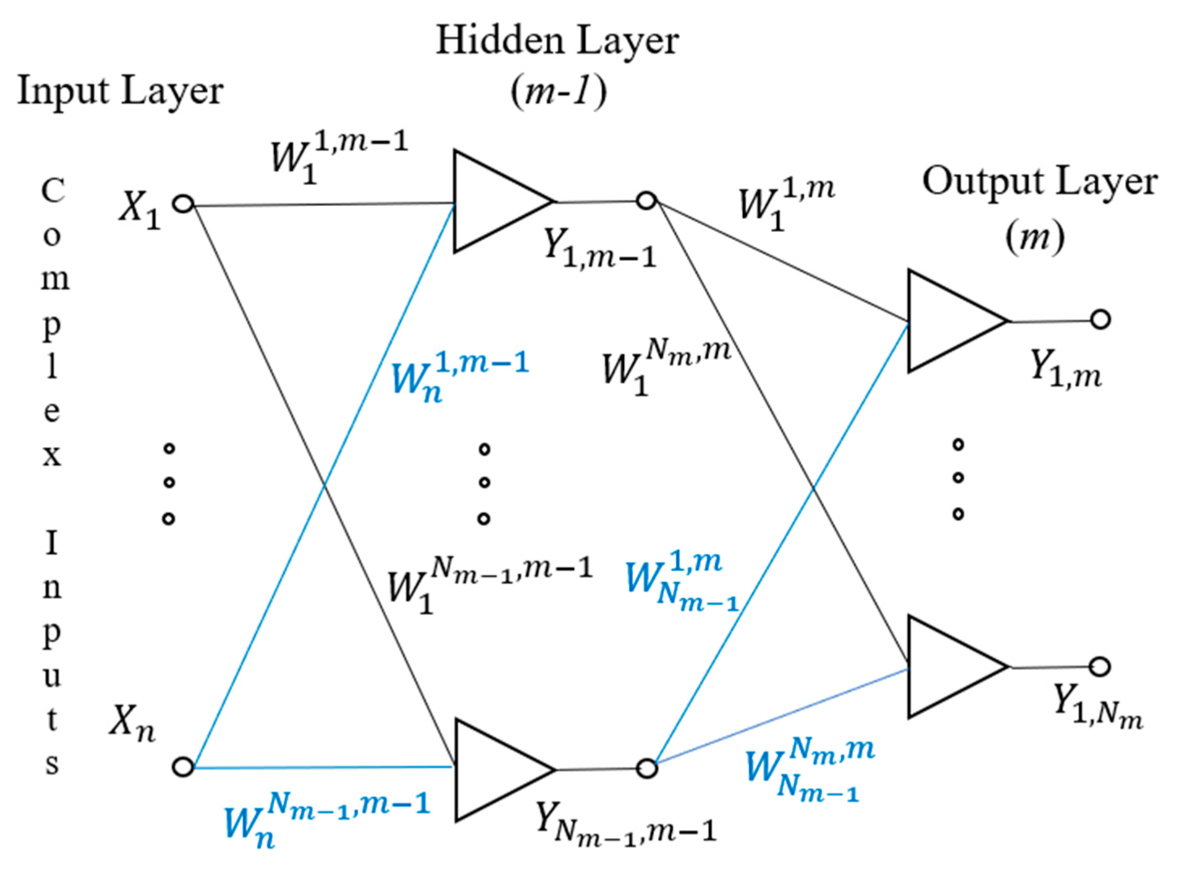
  • To propose and evaluate the use of an MLMVN in the classification of PQDs. This technique requires a frequency domain analysis based on the FT. The main advantage of the proposed method is its simple structure consisting of three layers and a small number of neurons in the hidden layer, leading to a very low computational effort and short learning time. In addition, since this neural network can directly process complex valued inputs, no coding operations are necessary.
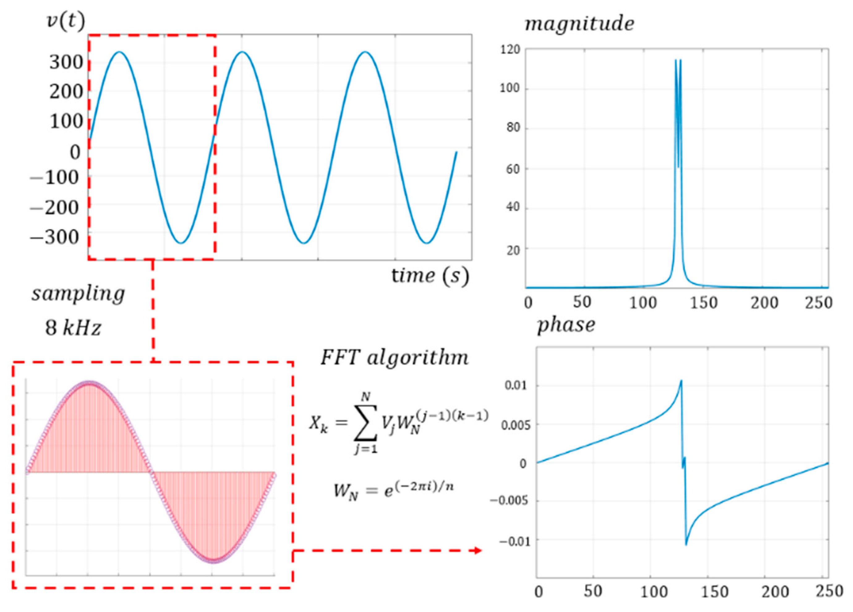
  • To propose and evaluate the performance of a convolutional neural network (CNN) with 2D convolutions in each layer for feature extraction from STFT coefficients. The main advantage of this solution with respect to the CNN in the literature is that the frequency component of the time signal is added to the input by means of a Fourier transform, thus adding one more dimension of information to the input signal and exploiting the CNN’s feature extraction capabilities.
  • To perform an extensive experimental validation of the previous techniques through a real test bench able to emulate the PQDs. The proposed test bench allows the automatic generation of a great variability in disturbances, simulating critical situations typical of industrial contexts with high precision.
The paper is organized as follows: in Section 2, the main theoretical aspects of the proposed classifiers are presented; in Section 3, the training results are shown; in Section 4, the experimental setup used to verify the performance of the two techniques is presented; Section 5 shows the experimental validation and highlights positive and negative aspects of the classifiers; in Section 5, the conclusions and future developments are reported.

2. Machine Learning Techniques

This section presents the main theoretical aspects of the two proposed classifiers and highlights the characteristics of the learning procedures. The MLMVN employed here contains three layers and allows the use of a reduced number of neurons in a single hidden layer, thus speeding up the learning phase and limiting the computational cost. Thanks to its complex nature, it can be easily used in the solution of electrical problems, where all quantities are expressed by phasors. The CNN in this paper is used in conjunction with the STFT to convert the 1D signal into a 2D matrix and extract its time–frequency components as in [29]. Additionally, this is done so the signal can be treated as an image, to exploit the feature extraction capabilities of this architecture and obtain the desired results. Furthermore, in many recent applications, CNNs are used in real time to classify signals of different natures [30], diagnose faults in various electrical machines [31], and predict the evolution of numerous systems and electrical quantities [32]. This has led to the development of many frameworks and toolboxes for real-time implementation, which allows for the immediate acquisition of signals and their classification.

2.1. Convolutional Neural Network Short-Time Fourier Transform

In this work, the use of CNNs was studied by means of an STFT. The STFT was used to extract the spectral component of the input voltage signal along with its temporal component. This was then used to classify the input voltage signal using the CNN. The STFT for classification using the CNNs has been previously used in other applications to improve CNN classification results, as shown [33,34,35]. CNNs are feedforward neural networks that use 2D convolutions in each layer for feature extraction and dimensionality reduction. The 2D convolution is:
S [ n 1 , n 2 ] = m 1 = 1 M 1 m 2 = 1 M 2 x [ m 1 , m 2 ] k [ n 1 m 1 , n 2 m 2 ]
The CNN works by adjusting the kernel denoted by parameter k during training to find the optimum kernel weights for the feature extraction of signal x for each corresponding filter in each convolutional layer. Figure 2 shows the function of the 2D convolutional layer where the kernel moves in a sliding window manner through the input matrix. A max pooling layer is then added to the convolutional layer to reduce the size of the image, extract the most important parts of the image, and reduce the training time. Pooling layers of a CNN implement a spatial dimensionality reduction operation designed to reduce the number of trainable parameters for the next layers and allow them to focus on larger areas of the input pattern [36]. The max pooling layer can be defined as the summary statistics of the output of the preceding convolutional layer. The max pooling layer identifies the maximum of a given section and sets it as the reduced output of the convolutional layer. Figure 3 describes the function of the max pooling layer in a CNN. Each section is denoted by a specific color: the maximum value of a section is the value of that specific section in the reduced output.
CNNs were originally created for image classification tasks. To create a 2D, image-like signal, the use of an STFT was explored to convert a 1D signal into a 2D matrix. This is done to exploit the CNN’s image feature extraction capabilities. The STFT is a discrete Fourier transform in a windowed section of the signal. The STFT permits frequency analysis in the time domain using a sliding window. The STFT is an enhanced mathematical methodology, derived from the discrete Fourier transform (DFT), to explore the instantaneous frequency as well as the instantaneous amplitude of localized waves with time-varying characteristics [34]. This method allows the time signal to be converted into a time–frequency signal i.e., a 2D matrix. Some of the disturbances in power quality studied in this work involve the injection of undesired frequency components (harmonics distortion and notch). The other disturbances involve the deviation of voltage levels from their nominal values, which can also be shown in the STFT. Figure 4 shows each converted disturbed voltage signal seen in Figure 1 with its time–frequency counterpart. The heatmap represents a yellow color for a high level of a frequency component and a blue color for a low level of a frequency component. In Figure 4, all signals have a high level at 50 Hz, which corresponds with the supply voltage frequency. The harmonic distortion and the notch show other frequency components, and the sag, swell, and interruption show a decrease or an increment in intensity at 50 Hz. The STFT is shown in (2), where x is the input signal and w is the window function. The window function used in this work is the Blackman window. The equation of the Blackman window is shown in (3), where a0 = (1 − α)/2, a1 = 1/2, a2 = α/2, and α = 0.16.
X [ m , n ] = k = 0 L 1 x [ k ] w [ k m ] e j 2 π n k / L
w [ n ] = a 0 a 1 c o s ( 2 π N ) + a 2 c o s ( 4 π N )
Since the classification task involves multiple classes, the CNN has the same number of classes as outputs. The output of the CNN involves a fully connected layer with six outputs. Each output represents each class. The output is then converted to a probabilistic density function by means of a SoftMax function. SoftMax functions are most often used as the output of a classifier with the aim of representing the probability distribution over n different classes [37]. The SoftMax function converts the output of each neuron into a probability using (4), where e x i is the exponential output of a given neuron and j = 1 K e x j is the sum of all the exponential outputs denoted by K. The sum of all the outputs of the SoftMax equals 1. Figure 5 shows an example of the SoftMax function which classified a given voltage signal with a probability of harmonic distortion of 99% and a probability of other disturbances of 0.2%.
P ( y ^ = j | x ) = e x i   j = 1 K e x j
Since this is a classification task and it is a multiclass problem, the loss function is a cross entropy loss shown in (5). In this formula, P ( y ^ i | x ) is the output of the SoftMax function and yi is the training label.
C E = i C y i l o g ( P ( y ^ i | x ) )
The gradient during training is calculated and the CNN is updated using the Adaptive Moment Optimizer (ADAM optimizer). The ADAM optimizer is an adaptive learning rate optimizer that uses first- and second-order moments of the gradients for updating the individual parameters. In this work, the input voltage signal was converted to a time–frequency matrix and then classified using the CNN. To achieve this, a dataset of voltage signals with disturbances was generated and transformed into its time–frequency counterpart using the STFT. The CNN was trained using the time–frequency dataset, obtaining a probability of each disturbance with the SoftMax function. Using the cross-entropy loss function, the output was measured with the labeled classes and the weights were adjusted using the ADAM optimizer.

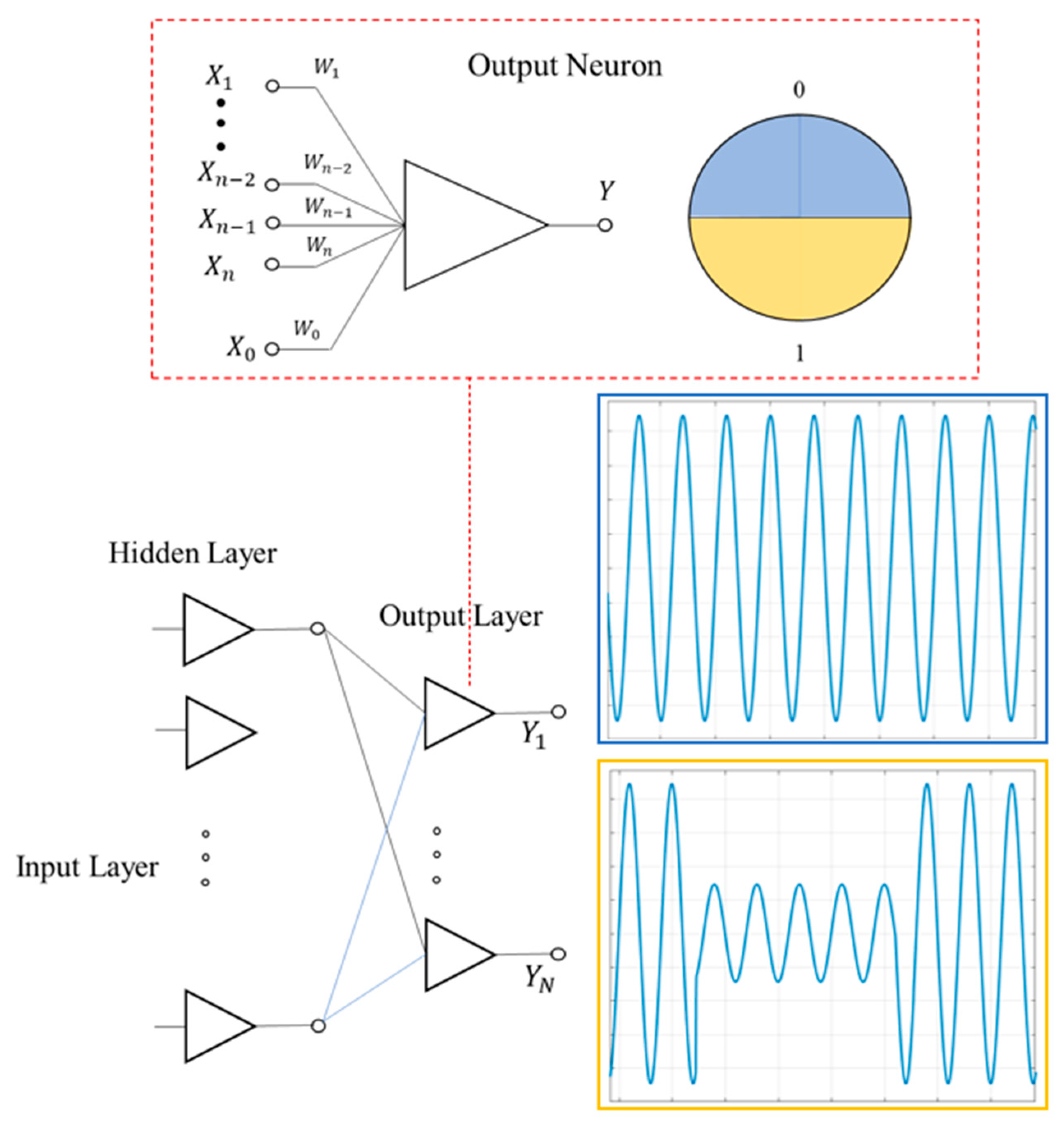
2.2. Multilayer Neural Network with Multivalued Neurons

One of the most innovative aspects presented in this paper is the use of an MLMVN in the classification of electrical disturbances. This paper represents the first application of a neural classifier based on multivalued neurons on the field of power quality evaluation. The MLMVN structure used in this work is the classic three-layer configuration presented in [38], while the use of binary neurons in the output layer, the introduction of the “Winner Takes All” rule, and the choice of processing complex coefficients obtained through the FFT of the sampled voltage waveforms are specific aspects of this application. This type of neural network is based on a feedforward neural network structure and a derivative free backpropagation procedure during the training phase [38]. The absence of derivative terms makes the correction of the weights very fast compared to other machine learning techniques. Additionally, the complex nature of the MLMVN makes it easily adaptable to electrical problems. In fact, the electrical quantities in power transmission and distribution grids are characterized by alternating waveforms and therefore are represented by phasors. Since each electrical standard has a single frequency value, line quantities can be expressed as complex numbers characterized by magnitude and phase. For these reasons, the MLMVN has been used with good results in failure prevention for electrical infrastructures [39] and analog circuits [40]. From a general point of view, this classifier is a three-layer neural network in which the elementary unit is the multivalued neuron (MVN) described in [38], and the inputs and weights are complex numbers. Figure 6 shows the global structure of the MLMVN where, for example, W i k , m is the i-th complex-valued weight of the k-th neuron belonging to the layer m, N m 1 is the number of the neurons belonging to the hidden layer, N m is the number of the neurons belonging to the output layer, and (X1, X2, …, Xn) are the complex-valued inputs.
In this paper, the complex-valued inputs (X1, X2, …, Xn) were obtained from the discrete Fourier transform (DFT) of the sampled line voltage with a frequency of 8 kHz. During the training phase, the time domain samples of the waveforms were processed using a fast Fourier transform (FFT) algorithm, and each complex term obtained was used as an input of the MLMVN. Figure 7 summarizes this procedure.
Since the correction of the weights is based on a supervised learning algorithm, many sample signals must be used with the corresponding desired classifications. Therefore, the structure of the dataset matrix used during the training phase is:
[ X 1 ( 1 )             X 2 ( 1 )         X n ( 1 )           0 X 1 ( N S )       X 2 ( N S )   X n ( N S )         5 ]
where the last column contains the indices of the fault classes, n is the number of points used in the fast Fourier transform algorithm, and NS is the total number of examples.
Each term Xk, with k = 1, …, n, is calculated as
X k = j = 1 N V j W N ( j 1 ) ( k 1 )
in which Vj is a voltage sample and WN is obtained using (8).
W N = e ( 2 π i ) / n
Once the complex-valued inputs are calculated, all the weights are initialized to random values and the dataset matrix shown in (6) is processed one row at a time. The element in the last column of each sample is used to calculate the corresponding desired output D, while the inputs (X1, X2, …, Xn) are processed through the two layers of neurons of the MLMVN. Neurons belonging to the hidden layer are characterized by a continuous activation function:
P ( z ) = e i   A r g ( z ) = z | z |
where z is the weighted sum of the inputs as follows:
z = W 0 + i = 1 n W i X i
where W0 is the weight of the bias input, Wi is the i-th weight of the considered neuron, and Xi represents the corresponding i-th input. On the other hand, the output layer of the MLMVN contains only discrete neurons, which have a finite number of possible outputs. Each of these neurons divides the complex plane into k equal sectors, and the output corresponds to the lower border of the sector containing z. From a mathematical point of view, given the total number of sectors k, the output of the neuron is equal to the lower limit of the j-th sector if the argument of the weighted sum is between 2π/k and 2π(j + 1)/k.
P ( Z ) = Y = ε k j = e i 2 π j / k         i f           2 π j / k arg ( z ) < 2 π ( j + 1 ) / k
Therefore, the combination of the output neurons is used to define the global classification results. In this sense, it is necessary to mention that the output neurons used in this paper are binary. This is a specific solution chosen for this kind of application which involves the use of a neuron for each electrical disturbance in the output layer. Therefore, each neuron has only two possible outputs: (1 + i0) or (−1 + i0). The first value corresponds to the lower border of the sector [0 π), while the second term is that of the interval [π, 2π). This setting allows the reduction in misclassifications between consequential sectors but requires the introduction of a specific method for selecting outputs. In fact, the single failure hypothesis is assumed, and this means that only one neuron can be activated by detecting the corresponding disturbance. If, during the training phase, more than one neuron is activated, the “Winner Takes All” rule is used. This means that only the neuron with the lowest error is kept in the activated state. Therefore, each output neuron is associated with a specific voltage disturbance, and the upper-half plane [0 π) is used to describe its absence, while the lower-half plane [π, 2π) is used to indicate the problem. For example, the first neuron belonging to the output layer focuses on sensing the voltage sag, as shown in Figure 8.
Therefore, one neuron for each disturbance is used in the output layer. To facilitate the interpretation of the results, the first sector of each output neuron is encoded by the value “0”, and the second sector by the value “1”. Table 3 summarizes the organization of the output layer.
As stated before, the MLMVN falls in the category of feedforward neural networks, and the training is performed in a supervised manner. The first step in this procedure is to map the correct combination of desired outputs to each example belonging to the dataset. All the outputs equal to “0” are converted into the complex number (1 + i0), while the outputs equal to “1” become (−1 + i0). These values are used to calculate output errors and initiate the backpropagation procedure. Given D k , m s , the desired output of the k-th neuron belonging to layer m obtained by processing the sample s (s = 1, …, Ns), the corresponding error is the difference between D k , m s and the current output Y k , m s .
These values are normalized with respect to the number of neurons of the previous layer as shown in (12).
δ k , m s = D k , m s Y k , m s N m 1 + 1
These errors, calculated on the output neurons, are backpropagated from the last layer to the input one through the mathematical rule presented in (13), as shown in [36].
δ k , m 1 s = 1 N m 1 + 1 i = 1 n m δ i , m s ( W k i , m ) 1
This standard correction procedure allows the adjustment of the weights by using (14),
Δ W i k , m = α k , m ( N m 1 + 1 ) | z k , m s | δ k , m s Y ¯ i , m 1 s
where Δ W i k , m is the correction for the i-th weight of the k-th neuron belonging to the layer m, α k , m is the corresponding learning rate, N m 1 is the number of the inputs equal to the number of outputs of the previous layer, z k , m s is the magnitude of the current weighted sum, δ k , m s is the output error, and Y ¯ i , m 1 s is the conjugate-transposed input for the output layer neurons and inner hidden layer neurons (if any) or a reciprocal input for the first hidden layer neurons. Equation (14) is used individually for each weight, and it represents the main difference between neural networks based on multivalued neurons (MVNs) and those based on real-valued neurons, because it does not contain derivative terms. This guarantees the low computational cost and very fast training phase of the MLMVN compared to other algorithms. To obtain a further reduction in the training time, the standard correction rules were replaced with a batch algorithm [41]. In this case, the output errors are calculated as shown in (12) and backpropagated as shown in (13) for each row of the dataset without adjusting the weights. Once all the examples belonging to the dataset have been processed and the corresponding errors have been defined, i.e., at the end of each training epoch, the corrections of the weights are calculated through a batch algorithm such as the QR decomposition. Each error is then saved in a specific matrix:
[ δ 1 , m 1   δ 2 , m 1 δ n , m 1 δ 1 , m 2   δ 2 , m 2 δ n , m 2                   δ 1 , m N S   δ 1 , m N S δ n , m N s ]
and a corresponding oversized system can be written as shown in (16), because the number of samples is greater than the number of corrections representing the unknowns.
Y ( Δ W k ) = δ k
This system must be solved through a linear least square (LLS), method obtaining the best corrections to meet the following condition,
Δ W k = a r g m i n Y ( Δ W k ) δ k 2 = Y * δ k
where the superscript k indicates the number of the neuron considered, Y * = ( Y T Y ) 1 Y T is the pseudo-inverse of the matrix Y, and YT is its conjugate transpose. In this work, QR decomposition is used, and the error matrix shown in (15) for the hidden layer consists of the backpropagated terms. To improve the classification performance of the MLMVN proposed in this paper, the “soft margin” rule was adopted [42]. In this case, the training phase is changed to bring the weighted sums as close as possible to the bisector of the desired sectors. This technique avoids the misclassification of the z-terms that fall close to the edge between two successive sectors. From the computational point of view, there are no differences compared to the standard procedure, because the only change is the use of bisectors as desired outputs D k , m s . Therefore, the goal of the weight correction is not only the positioning of the output in the correct sector, but also the minimization of the distance with respect to the bisector of that sector.

3. Training Results

This section presents the main results obtained during the training phase of the machine learning techniques described above. The data used during the training phase were generated by a simulation procedure on Matlab and Simulink environments. Therefore, a Matlab script was used to create a large variability in electrical disturbances in a very short time, starting from the sinusoidal function of the line voltage, which is characterized by a frequency of (50 Hz ± 0.2%) and a root mean square value of 230 V. The amplitude and the frequency components of these signals were modified to create all the different disturbances following the formal definitions presented in Section 1. Starting from the normal sinusoidal signal shown in Figure 1a, the value of the maximum amplitude was chosen randomly in the interval (23 ÷ 207) V to simulate the presence of a voltage sag. This problem, in fact, causes a reduction in the phase voltage between 10% and 90% of the nominal value. Similarly, examples of voltage swell were created by considering increases in the maximum amplitude from 10% to 50% of the nominal value. As for the harmonic disturbances, signals with frequencies multiple of the fundamental frequency (50 Hz) were generated up to the eleventh harmonic and then added to the line voltage. Notch is a condition when the magnitude of voltage decreases towards zero for a short period of time, usually microseconds. This condition was simulated in Matlab by adding impulsive components at specific instants of the nominal voltage waveform. Finally, interruptions were simulated by reducing the maximum voltage value below 10% of the nominal value. Note that the voltage frequency variations considered acceptable by the technical standard CEI EN 50160 were included in the formation of the dataset, and this means that the classifiers are robust with respect to these perturbations, which do not represent power quality problems.
Furthermore, other examples of PQDs were generated through the Simulink model proposed in [29] by the authors. In this way, it was possible to simulate, with a high level of accuracy, distortions caused by faults in low-voltage distribution networks. A waveform with a duration of three periods (60 ms) was created for each signal, and 250 examples were generated for each fault class (nominal condition, voltage sag, voltage swell, harmonic distortion, notch, and interruption). A total of 200 of these examples were generated using the Matlab script, and the remaining 50 using Simulink. Therefore, a set of 1500 simulated signals were used to train the neural classifiers described above. The simulated voltage waveforms were sampled with a frequency of 8 kHz, resulting in 480 samples for each example. These data were used to create two matrices ensuring the properties presented in Section 2. In order to clearly show the results obtained for each PQ disturbance taken into consideration, the hold-out validation technique was used, and this means that the training procedure was divided into two phases: a learning phase and a validation phase. During the learning phase, 80% of the dataset was chosen randomly and used for the correction of the weights. Subsequently, the remaining 20% was used in validation to verify the classification results. In both phases, the index used to evaluate the performance is called the Classification Rate (CR), and it corresponds to the ratio of correctly classified samples to the total number of processed samples. The comparison between these two classification results is the basis of the heuristic approach used to define the structure of the classifiers avoiding overfitting problems. Additionally, to provide accurate performance evaluation, the hold-out validation results shown in the following subsections were verified through a cross-validation method. This means that the division of the dataset described above was repeated five times to use all the data both in the learning phase and in the validation phase. The overall classification rate was then analyzed to identify limits in the generalization capabilities.

3.1. Training CNN-STFT
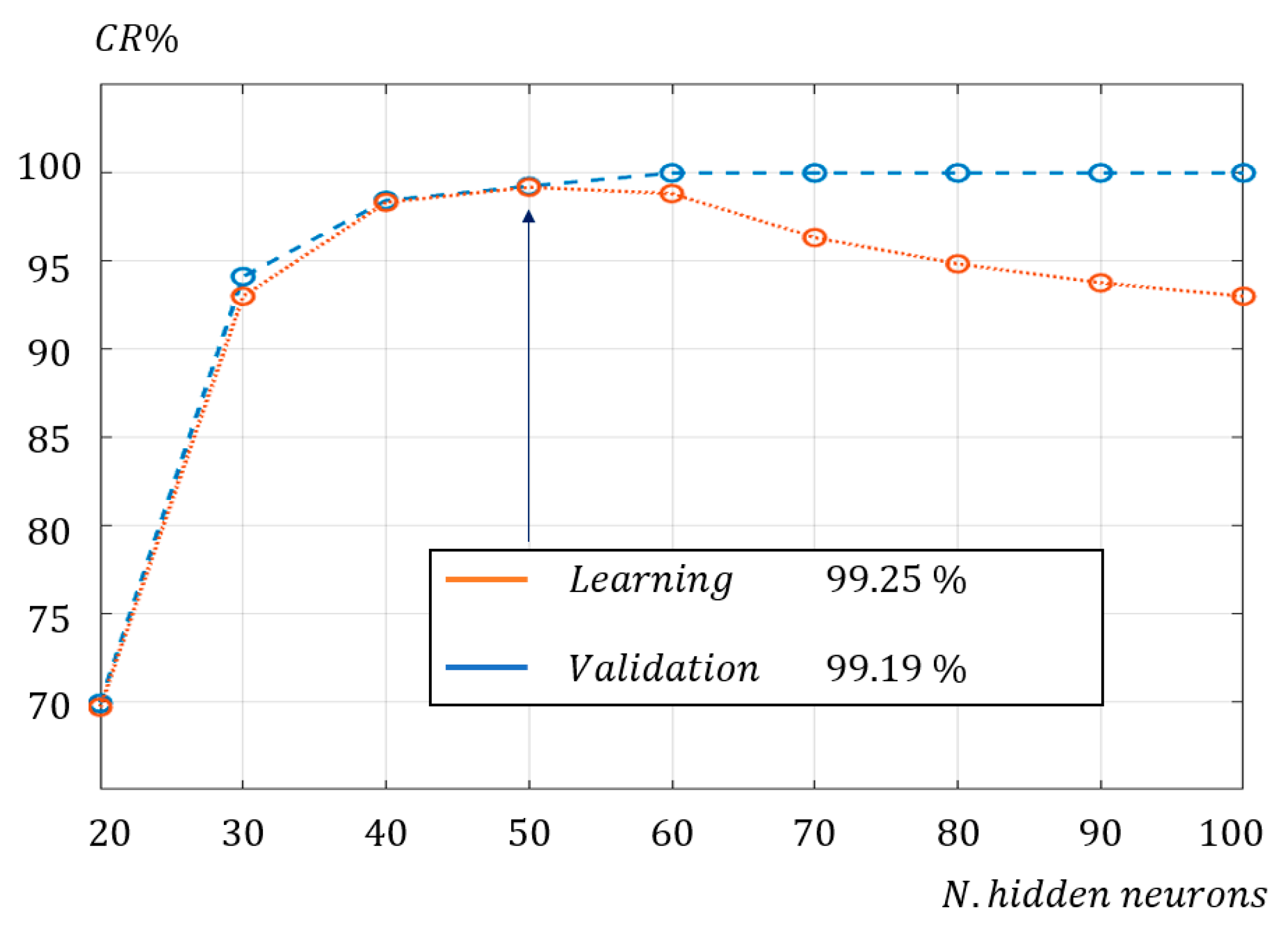
The CNN training procedure requires a dataset containing the electrical voltage disturbance in their time–frequency domain. Therefore, the simulated voltage disturbances were converted to their time–frequency domains via the STFT, as shown in Section 2.1. The used CNN architecture has an input of 500 rows and 5 columns. This means 500 frequency components and 5 cycles. The CNN reduces the input using the max pooling layers and at the same time increases the filter size. The training was completed, and the precision and recall were calculated for each class. The precision of the CNN resulted in 100% in all classes except the normal, which had a classification rate of 99.3% with the training data and 98.9% with the validation data. The results are shown in Table 4. The recall resulted in a 100% classification rate in all except for the sag and swell, which resulted in 99.6% and 99.7%, respectively, for the training, and 99.7% and 99.2%, respectively, for the validation. The results are shown in Table 5. The CNN has an overall accuracy of 99.89% for the training dataset and overall accuracy of 99.82% for the validation dataset.
The idea of using the CNN in this work is to take advantage of the already-developed frameworks and toolboxes to incorporate in a real-time environment. These frameworks already optimize the classification process in a deep learning pipeline. As shown in Figure 9 and Figure 10, the proposed method has lower memory space requirements than already implemented architectures, obtaining a high accuracy in the classification process. Due to the use of a fully connected layer, the CNN-STFT has a high number of parameters that makes it slow in the training process, but it has a low number of layers, which makes it faster than the other architectures for classification in a real-time environment.

3.2. Training MLMVN

The MLMVN training procedure requires a matrix-like dataset, shown in (6), containing a large variability in electrical disturbances expressed in the frequency domain. Therefore, the discrete Fourier transform was applied using a fast Fourier transform algorithm to the samples of the voltage waveforms generated in Matlab. In this paper, 256 points were considered for the DFT, and the corresponding complex values were used as inputs of the MLMVN. Table 6 summarizes the results obtained using 50 neurons in the hidden layer of the MLMVN. As stated before, the output layer contains five binary neurons, one for each electrical disturbance, and the nominal conditions correspond to a combination of five zeros.
Note that the size of the hidden layer was chosen by comparing the classification rate of the learning phase and that of the validation phase as the number of hidden neurons varies. The results of this heuristic approach are shown in Figure 11. When the classification results of the learning phase are excellent but those of the validation phase decrease, this situation can be considered as an index of overfitting. Therefore, it is necessary to reduce the number of neurons in the hidden layer. Finally, it should be noted that the results reported in Table 5 are also confirmed through the cross-validation method. In fact, by repeating the training procedure five times while modifying the data used for learning and validation, the overall classification rate obtained is 98.94%.
Before proceeding to the experimental validation of the performances, during the training phase, a comparison was proposed with some computational intelligence techniques derived from those reported in Table 2. Some of these results are shown in Table 7.

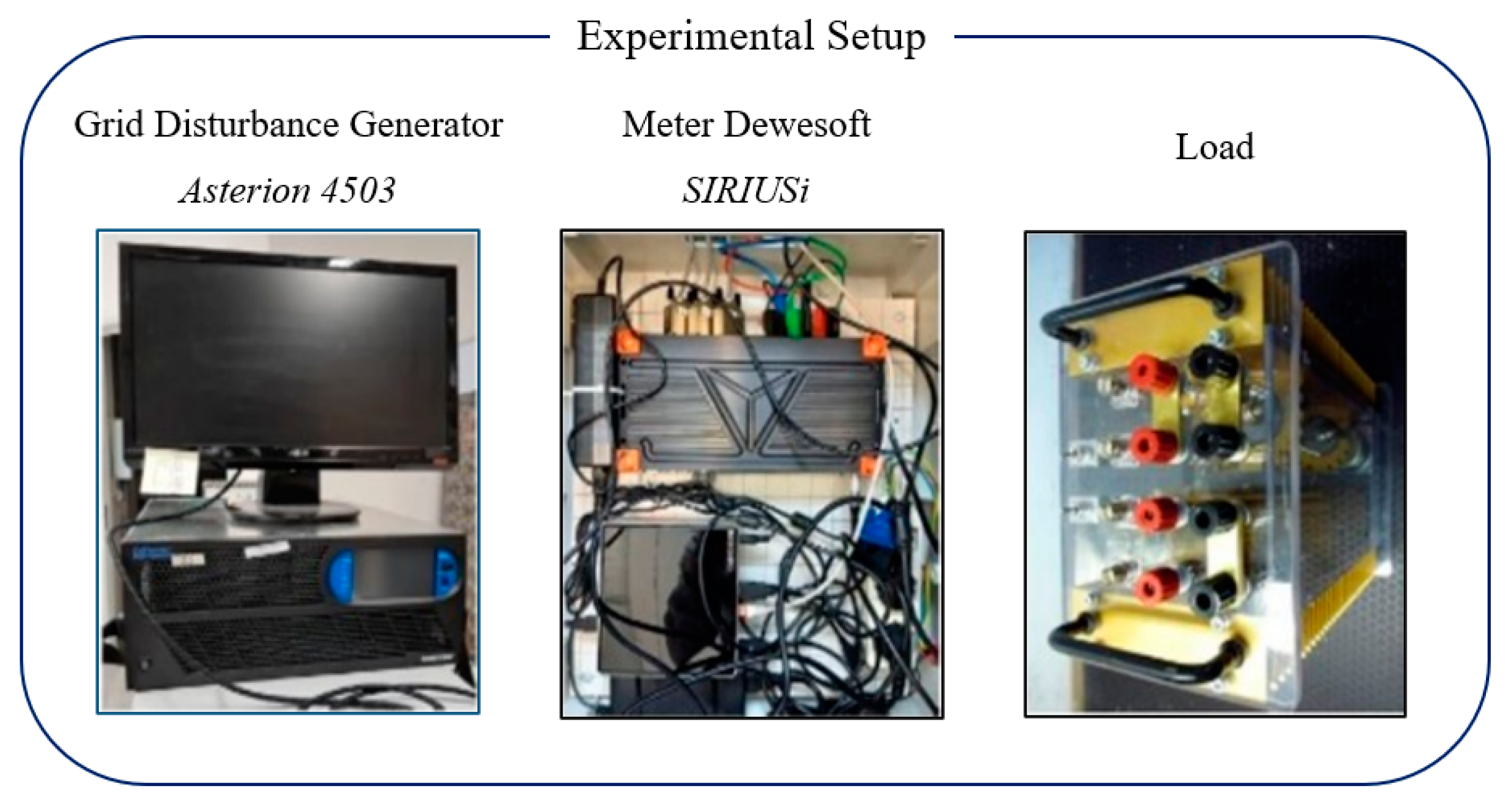
4. Experimental Setup

The experimental testing of the training results was carried out by generating an experimental dataset of the electrical quantities of interest. These datasets contain phase voltages and currents and some derived quantities that are needed for the disturbance recognition. Once the dataset was generated, it was fed to the classification algorithm for testing.
The experimental setup is shown in Figure 12. The proposed setup can reproduce multiple network disturbances with different spectral contents, durations, and amplitudes, allowing us to evaluate the detection accuracy of the proposed neural networks. To simulate a grid with power quality disturbances, the Asterion 4503 A1/3PH by Ametek programmable AC source was used. It has a maximum power of 4500 VA and can generate arbitrary waveforms at a frequency of up to 5 kHz. Its dynamic characteristics allow the simulation of any type of network disturbance. To acquire the current and voltage waveforms, a SIRIUSi-HS-4xHV-4xLV was used. The acquisition system can acquire eight channels at a maximum sampling rate of 50 kHz. The purpose of the experimental setup was to reproduce most of the power quality disturbances that may affect industrial plant and to guarantee the repeatability of the electrical dynamics and accuracy of the measurements for each experiment so that the comparison is consistent. Moreover, thanks to the flexibility of the systems used, it can be adapted to any new configuration required for the testing of detection and classification algorithms.

5. Experimental Validation of the Classification Techniques

This section proposes further validation by using real voltage measurements to highlight the advantages and disadvantages of both techniques. Therefore, different examples of disturbances were generated by the two experimental setups described above, and the corresponding voltage waveforms were sampled with a frequency of 8 kHz. Finally, a comparison of a specific sequence of electrical disturbances is presented.

5.1. Validation of the MLMVN with Real Measurements

The first voltage waveform used to validate the performance of the MLMVN-based classifier is shown in Figure 13, where the voltage sags and nominal conditions alternate with different durations.
The time window proposed in Figure 13 has a duration of five seconds and, therefore, it contains 250 sinusoidal periods, each of which is made up of 8000 samples. One of the most important aspects in the evaluation of classification results is taking the time interval into consideration. For example, the signal shown in Figure 14 can be processed using five consecutive time intervals of one-second durations. The proposed monitoring method assesses the DFT for each interval and classifies them. As shown in Figure 14, this procedure allows the perfect classification of the considered voltage waveform. Note that the second time window, 1 to 2 s, is correctly classified as sag because the perturbation affects the initial part of this observation.
However, there are some situations in which the MLMVN misclassifies, for example in the case of a brief perturbation. Figure 15 describes this condition: the time interval taken into consideration is classified as normal, but it presents a voltage sag of 60 ms.
To overcome this limitation, it is possible to reduce the duration of the time interval used for the classification procedure. In this way, short disturbances are identified with a high classification accuracy, and the exact moment they start is detected. Figure 16 shows a classification example in which a voltage waveform is processed using 60 ms time intervals. Note that the excellent classification results shown in Figure 16 can also be obtained by considering the other fault classes. Table 8 summarizes the classification performances obtained using different time interval durations.
These results were obtained considering real voltage measurements of 25 s, and they confirmed the excellent performance when the waveform is processed using a short time interval. On the other hand, the classification rate decreases as the number of periods processed simultaneously increases. It should be noted that the classification of the harmonic disturbance is slightly better than that of the other perturbations when using time intervals of 1 s and 2 s. The reason for this result is that the presence of a voltage component with frequency higher than 50 Hz introduces significant variation in the Fourier analysis. As shown in Figure 17, in the magnitude representation, several lines are introduced with respect to the normal condition, each of which corresponds to a frequency component. These contributions are also present in the case of a short-duration harmonic perturbation and therefore make the classification slightly easier. As for the other voltage disturbances, they focus on the 50 Hz component, and this makes it difficult to recognize brief problems.
In addition, it should be noted that some of the errors in detecting voltage sags and interruptions using a short time interval (0.006 s) correspond to class 4 misclassifications. In fact, in the instant in which the voltage drop begins, features very similar to those of a notch can occur. This means that the MLMVN can detect the starting point of these disturbances, but sometimes classifies it as a notch. Figure 18 describes this situation. Without considering these errors, the classification rate would be over 99%.

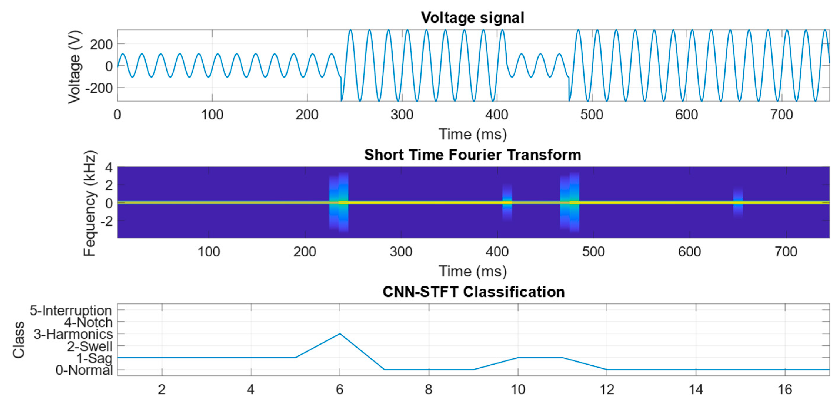
5.2. Validation of the CNN-STFT with Real Measurements

The same voltage waveform described in the previous section was used to validate the performance of the CNN-based classifier shown in Figure 2, where the voltage sags and nominal conditions alternate with different durations using the voltage disturbance generator. For the validation of the CNN, the signal was converted to its time–frequency domain using the STFT and then classified as a 500 × 5 image. The dimensions of the time–frequency matrix represent 250 frequency components of 3 cycles, or 60 ms, with a sliding window of half a cycle, which makes 5 DFT. The validation of the CNN-STFT resulted in 4 misclassifications out of 479 classifications, which makes it 99.16%accurate. Misclassifications in this experiment occurred in transitions between normal and sag or sag and normal. This is due to high-frequency components being found at each transition, which led to a harmonic classification. Figure 19, Figure 20, Figure 21 and Figure 22 show the classification results. The top plot shows the voltage signal to be transformed and classified. All figures show at least one sag that transitions to normal or vice versa. As shown in the STFTs, the transitions create high-frequency components which often lead to a harmonic classification, as shown in Figure 19, Figure 20, Figure 21 and Figure 22.

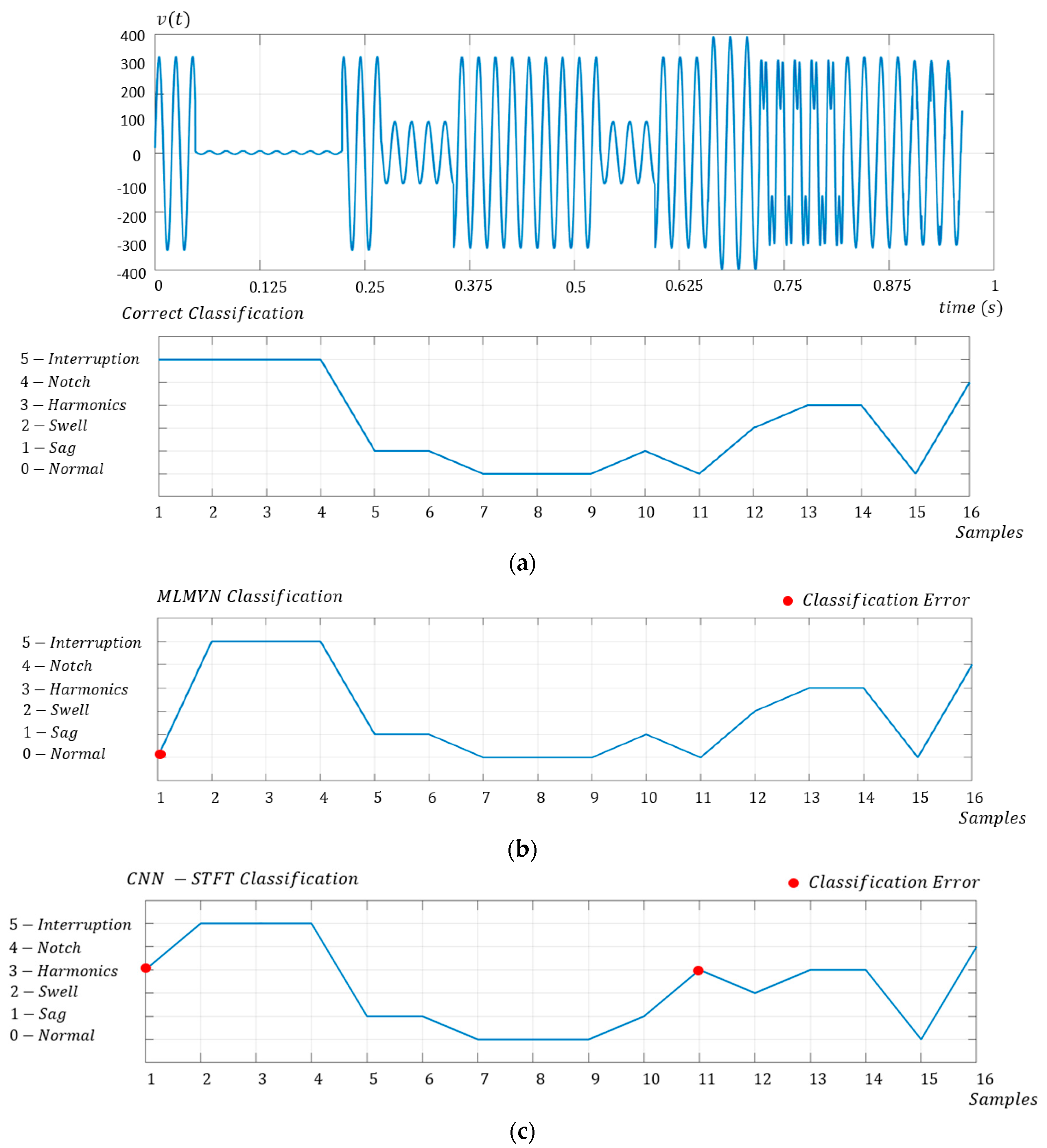
5.3. Comparison between MLMVN and CNNSTFT

Finally, a comparison between CNN-STFT- and MLMVN-based classifiers is presented. For this comparison, a voltage signal containing all five categories of disturbances was generated. The rated voltage value is that of the Italian distribution network (Vrms = 230 V, f = 50 Hz).
This signal was generated as shown in Section 4 and sampled with a frequency of 8 kHz. The goal of the classification is to determine the power quality by studying 60 ms (three cycles) at a time. Therefore, the sampled signal was divided into groups of 480 samples, and each of them was assigned the corresponding classification. Figure 23a shows the overall signal and the correct classification of the 16 groups of the analyzed samples, while Figure 23b,c present the classification results obtained through the two techniques.
The MLMVN-based classifier misclassified in the first sample. This is a very complex situation to recognize because the voltage sag situation occurs in the last half-period of the three taken into consideration. Figure 24 shows this situation. It can be said that by using one FT for each sine cycle, i.e., by analyzing one cycle at a time, this type of error can be eliminated, ensuring 100% accuracy.
It is necessary to highlight that the experimental data were also used to evaluate the robustness of the classifiers with respect to the measurement noise. Therefore, random noise signals were added to all the real measurements taken into consideration, obtaining signal-to-noise ratios between 20 dB and 50 dB. The classification performance decreases as the noise increases, but both classifiers are robust and guarantee an overall classification rate greater than 82%, even in the worst case.
In conclusion, a consideration of the classification techniques presented in Table 8 can be introduced. The two techniques that offer the best results during the training phase were used on the experimental data. Both the quadratic SVM and the AlexNet show excellent performance on four fault classes, while misclassifying all examples of nominal conditions with notch type disturbances.
As for the CNN-STFT, the transition from normal to a disturbance results in a high-frequency component which can be interpreted as another disturbance, as shown in the previous section. This is also the cause of the errors presented in Figure 23. Figure 25 shows a comparison of the STFT of two waveforms: the left side of the figure shows the STFT of a normal signal generated with the noise generator, while that of a sag is shown in the right side. The transitions shown on the image inject high-frequency harmonic components that, in some instances, disrupt the classification process, leading to some misclassifications in the validation. Comparing the results obtained with those of some important works in the literature, such as [43,44], it is noted that the performance in the case of individual disorders is comparable. In fact, classification results higher than 98% are obtained for the individual fault classes. Further modifications in the output layers of the two proposed algorithms will be implemented to deal with multiple failures, as in [26,27,28].

6. Conclusions

In conclusion, it can be stated that the two proposed techniques allow the monitoring of the power quality in a low-voltage distribution network with an excellent level of accuracy. The short training time and the use of common techniques, such as the Fourier transform, in the data processing phase make the two classifiers very versatile and easily adaptable for the recognition of other electrical disturbances.
Compared to other techniques, they allow the analysis and classification of a voltage signal in time and frequency. This can further enhance the feature extraction capabilities due to the addition of the frequency dimension. The use of the STFT was to transform the 1D signal into a 2D matrix to exploit the CNN’s feature extraction capabilities and its benefits for classification tasks. The STFT was chosen in this work because it uses a discrete Fourier transform, which is a simple algorithm to implement in a real-time application compared to other time–frequency transformation algorithms.
Future developments could be focused on improving performance when processing a larger number of cycles per classification and introducing additional types of disturbances that are very frequent in industry. Furthermore, the real-time applications of these two approaches will certainly be studied in the future to develop an effective monitoring tool for electric grids. Therefore, the possibility of integrating the proposed techniques in embedded electronics and directly classifying the quality of the voltage waveform will be studied. This will certainly make the two techniques usable together with other systems for improving energy quality. To adapt the proposed classifiers to different acquisition devices in many other electrical systems, a measurement noise treatment will be introduced during the training phase. Finally, a very interesting future development will be improving neural algorithms to work under multiple failure hypotheses to classify disturbances consisting of multiple distortions.

Author Contributions

Conceptualization, C.A.I.G., M.B. and F.C.; methodology, A.L.; software, C.A.I.G. and I.A.; validation, F.G.; formal analysis, M.C.P.; investigation, F.C.; data curation, M.B.; writing—original draft preparation, C.A.I.G., M.B. and F.C.; writing—review and editing, M.C.P. and A.L.; visualization, F.G. and L.P. All authors have read and agreed to the published version of the manuscript.

Funding

This research received no external funding.

Data Availability Statement

No new data were created or analyzed in this study. Data sharing is not applicable to this article.

Conflicts of Interest

The authors declare no conflict of interest.

References

  1. Wang, L.; Qin, Z.; Slangen, T.; Bauer, P.; van Wijk, T. Grid Impact of Electric Vehicle Fast Charging Stations: Trends, Standards, Issues and Mitigation Measures—An Overview. IEEE Open J. Power Electron. 2021, 2, 56–74. [Google Scholar] [CrossRef]
  2. Farhoodnea, M.; Mohamed, A.; Shareef, H.; Zayandehroodi, H. Power quality impacts of high-penetration electric vehicle stations and renewable energy-based generators on power distribution systems. Meas. J. Int. Meas. Confed. 2013, 46, 2423–2434. [Google Scholar] [CrossRef]
  3. BS EN 50160:2007; Voltage Characteristics of Electricity Supplied by Public Distribution Systems. Belgian Standard: Brussels, Belgium, 1994.
  4. Document IEC 61000-4-30; Testing and Measurement Techniques Power Quality Measurement Methods. IEC: London, UK, 2003.
  5. Standard 1159–2009; IEEE Recommended Practice for Monitoring Electric Power Quality. IEEE: Piscataway, NJ, USA, 2009.
  6. Zheng, Y.; Meng, F.; Liu, J.; Guo, B.; Song, Y.; Zhang, X.; Wang, L. Fourier Transform to Group Feature on Generated Coarser Contours for Fast 2D Shape Matching. IEEE Access 2020, 8, 90141–90152. [Google Scholar] [CrossRef]
  7. Qiu, W.; Tang, Q.; Liu, J.; Yao, W. An Automatic Identification Framework for Complex Power Quality Disturbances Based on Multifusion Convolutional Neural Network. IEEE Trans. Ind. Inform. 2000, 16, 3233–3241. [Google Scholar] [CrossRef]
  8. Garrido, M. The Feedforward Short-Time Fourier Transform. IEEE Trans. Circuits Syst. II Express Briefs 2016, 63, 868–872. [Google Scholar] [CrossRef]
  9. Zhao, B.; Li, Q.; Lv, Q.; Si, X. A Spectrum Adaptive Segmentation Empirical Wavelet Transform for Noisy and Nonstationary Signal Processing. IEEE Access 2021, 9, 106375–106386. [Google Scholar] [CrossRef]
  10. Santoso, S.; Powers, E.J.; Grady, W.M.; Parsons, A.C. Power quality disturbance waveform recognition using wavelet-based neural classifier. I. Theoretical foundation. IEEE Trans. Power Deliv. 2000, 15, 222–228. [Google Scholar] [CrossRef]
  11. Lin, W.; Wu, C.; Lin, C.; Cheng, F. Detection and Classification of Multiple Power-Quality Disturbances With Wavelet Multiclass SVM. IEEE Trans. Power Deliv. 2008, 23, 2575–2582. [Google Scholar] [CrossRef]
  12. Bíscaro, A.A.P.; Pereira, R.A.F.; Kezunovic, M.; Mantovani, J.R.S. Integrated Fault Location and Power-Quality Analysis in Electric Power Distribution Systems. IEEE Trans. Power Deliv. 2016, 31, 428–436. [Google Scholar] [CrossRef]
  13. Reaz, M.B.I.; Choong, F.; Sulaiman, M.S.; Mohd-Yasin, F.; Kamada, M. Expert System for Power Quality Disturbance Classifier. IEEE Trans. Power Deliv. 2007, 22, 1979–1988. [Google Scholar] [CrossRef]
  14. Lee, I.W.C.; Dash, P.K. S-transform-based intelligent system for classification of power quality disturbance signals. IEEE Trans. Ind. Electron. 2003, 50, 800–805. [Google Scholar] [CrossRef]
  15. Cai, K.; Cao, W.; Aarniovuori, L.; Pang, H.; Lin, Y.; Li, G. Classification of Power Quality Disturbances Using Wigner-Ville Distribution and Deep Convolutional Neural Networks. IEEE Access 2019, 7, 119099–119109. [Google Scholar] [CrossRef]
  16. Mahela, P.; Shaik, A.G.; Khan, B.; Mahla, R.; Alhelou, H.H. Recognition of Complex Power Quality Disturbances Using S-Transform Based Ruled Decision Tree. IEEE Access 2020, 8, 173530–173547. [Google Scholar] [CrossRef]
  17. Martinez-Figueroa, G.D.J.; Morinigo-Sotelo, D.; Zorita-Lamadrid, A.L.; Morales-Velazquez, L.; Romero-Troncoso, R.D.J. FPGA-Based Smart Sensor for Detection and Classification of Power Quality Disturbances Using Higher Order Statistics. IEEE Access 2017, 5, 14259–14274. [Google Scholar] [CrossRef]
  18. Janik, P.; Lobos, T. Automated classification of power-quality disturbances using SVM and RBF networks. IEEE Trans. Power Deliv. 2006, 21, 1663–1669. [Google Scholar] [CrossRef]
  19. Gong, R.; Ruan, T. A New Convolutional Network Structure for Power Quality Disturbance Identification and Classification in Micro-Grids. IEEE Access 2020, 8, 88801–88814. [Google Scholar] [CrossRef]
  20. Valtierra-Rodriguez, M.; de Jesus Romero-Troncoso, R.; Osornio-Rios, R.A.; Garcia-Perez, A. Detection and Classification of Single and Combined Power Quality Disturbances Using Neural Networks. IEEE Trans. Ind. Electron. 2014, 61, 2473–2482. [Google Scholar] [CrossRef]
  21. Yang, Z.; Liao, W.; Liu, K.; Chen, X.; Zhu, R. Power Quality Disturbances Classification Using A TCN-CNN Model. In Proceedings of the 2022 7th Asia Conference on Power and Electrical Engineering (ACPEE), Hangzhou, China, 15–17 April 2022; pp. 2145–2149. [Google Scholar] [CrossRef]
  22. Yoon, D.-H.; Yoon, J. Deep Learning-Based Method for the Robust and Efficient Fault Diagnosis in the Electric Power System. IEEE Access 2022, 10, 44660–44668. [Google Scholar] [CrossRef]
  23. Turizo, S.; Ramos, G.; Celeita, D. Voltage Sags Characterization Using Fault Analysis and Deep Convolutional Neural Networks. IEEE Trans. Ind. Appl. 2022, 58, 3333–3341. [Google Scholar] [CrossRef]
  24. Balouji, E.; Salor, Ö.; McKelvey, T. Deep Learning Based Predictive Compensation of Flicker, Voltage Dips, Harmonics and Interharmonics in Electric Arc Furnaces. IEEE Trans. Ind. Appl. 2022, 58, 4214–4224. [Google Scholar] [CrossRef]
  25. Machlev, R.; Perl, M.; Belikov, J.; Levy, K.Y.; Levron, Y. Measuring Explainability and Trustworthiness of Power Quality Disturbances Classifiers Using XAI—Explainable Artificial Intelligence. IEEE Trans. Ind. Inform. 2022, 18, 5127–5137. [Google Scholar] [CrossRef]
  26. Da Costa Pinho, A.; Gecildo, E.; Garcia, A. Wavelet spectral analysis and attribute ranking applied to automatic classification of power quality disturbances. Electr. Power Syst. Res. 2022, 206, 107827. [Google Scholar] [CrossRef]
  27. Gao, Y.; Li, Y.; Zhu, Y.; Wu, C.; Gu, D. Power quality disturbance classification under noisy conditions using adaptive wavelet threshold and DBN-ELM hybrid model. Electr. Power Syst. Res. 2022, 204, 107682. [Google Scholar] [CrossRef]
  28. Shafiullah, M.; Khan, M.A.M.; Ahmed, S.D. Chapter 11—PQ disturbance detection and classification combining advanced signal processing and machine learning tools. In Power Quality in Modern Power Systems; Academic Press: Cambridge, MA, USA, 2021; pp. 311–335. [Google Scholar] [CrossRef]
  29. Garcia, C.I.; Grasso, F.; Luchetta, A.; Piccirilli, M.C.; Paolucci, L.; Talluri, G. A comparison of power quality disturbance detection and classification methods using CNN, LSTM and CNN-LSTM. Appl. Sci. 2020, 10, 6755. [Google Scholar] [CrossRef]
  30. Cetin, R.; Gecgel, S.; Kurt, G.K.; Baskaya, F. Convolutional Neural Network-Based Signal Classification in Real Time. IEEE Embed. Syst. Lett. 2021, 13, 186–189. [Google Scholar] [CrossRef]
  31. Liu, X.; Zhou, Q.; Shen, H. Real-time Fault Diagnosis of Rotating Machinery Using 1-D Convolutional Neural Network. In Proceedings of the 2018 5th International Conference on Soft Computing & Machine Intelligence (ISCMI), Nairobi, Kenya, 21–22 November 2018; pp. 104–108. [Google Scholar] [CrossRef]
  32. Adhikari, A.; Naetiladdanon, S.; Sangswang, A. Real-Time Short-Term Voltage Stability Assessment using Temporal Convolutional Neural Network. In Proceedings of the 2021 IEEE PES Innovative Smart Grid Technologies—Asia (ISGT Asia), Brisbane, Australia, 5–8 December 2021; pp. 1–5. [Google Scholar] [CrossRef]
  33. Chen, Z.; Xu, Y.-Q.; Wang, H.; Guo, D. Deep STFT-CNN for Spectrum Sensing in Cognitive Radio. IEEE Commun. Lett. 2021, 25, 864–868. [Google Scholar] [CrossRef]
  34. Huang, J.; Chen, B.; Yao, B.; He, W. ECG Arrhythmia Classification Using STFT-Based Spectrogram and Convolutional Neural Network. IEEE Access 2019, 7, 92871–92880. [Google Scholar] [CrossRef]
  35. Nie, J.; Xiao, Y.; Huang, L.; Lv, F. Time-Frequency Analysis and Target Recognition of HRRP Based on CN-LSGAN, STFT, and CNN. Complexity 2021, 2021, 6664530. [Google Scholar] [CrossRef]
  36. Ñanculef, R.; Radeva, P.; Balocco, S. Training Convolutional Nets to Detect Calcified Plaque in IVUS Sequences. In Intravascular Ultrasound: From Acquisition to Advanced Quantitative Analysis; Elsevier: Amsterdam, The Netherlands, 2020; pp. 141–158. [Google Scholar] [CrossRef]
  37. Goodfellow, I.; Bengio, Y.; Courville, A. Deep Learning Ian. Foreign Aff. 2012, 91, 1689–1699. [Google Scholar]
  38. Aizenberg, I. Complex-Valued Neural Networks with Multi-Valued Neurons; Springer: New York, NY, USA, 2011. [Google Scholar]
  39. Aizenberg, I.; Belardi, R.; Bindi, M.; Grasso, F.; Manetti, S.; Luchetta, A.; Piccirilli, M.C. Failure Prevention and Malfunction Localization in Underground Medium Voltage Cables. Energies 2021, 14, 85. [Google Scholar] [CrossRef]
  40. Aizenberg, I.; Belardi, R.; Bindi, M.; Grasso, F.; Manetti, S.; Luchetta, A.; Piccirilli, M.C. A Neural Network Classifier with Multi-Valued Neurons for Analog Circuit Fault Diagnosis. Electronics 2021, 10, 349. [Google Scholar] [CrossRef]
  41. Aizenberg, I.; Luchetta, A.; Manetti, S. A modified learning algorithm for the multilayer neural network with multi-valued neurons based on the complex QR decomposition. Soft Comput. 2012, 16, 563–575. [Google Scholar] [CrossRef]
  42. Aizenberg, I. MLMVN With Soft Margins Learning. IEEE Trans. Neural Netw. Learn. Syst. 2014, 25, 1632–1644. [Google Scholar] [CrossRef]
  43. Borges, F.A.S.; Fernandes, R.A.S.; Silva, I.N.; Silva, C.B.S. Feature Extraction and Power Quality Disturbances Classification Using Smart Meters Signals. IEEE Trans. Ind. Inform. 2016, 12, 824–833. [Google Scholar] [CrossRef]
  44. Manikandan, M.S.; Samantaray, S.R.; Kamwa, I. Detection and Classification of Power Quality Disturbances Using Sparse Signal Decomposition on Hybrid Dictionaries. IEEE Trans. Instrum. Meas. 2015, 64, 27–38. [Google Scholar] [CrossRef]
Figure 1. Disturbance classes. (a) Normal. (b) Sag. (c) Swell. (d) Harmonics. (e) Notch. (f) Interruption.
Energies 16 03627 g001
Figure 2. Convolutional layer example where x is the input, k is the kernel, and y is the output.
Energies 16 03627 g002
Figure 3. Max pooling layer example where the input to the layer is reduced to the statistical summary.
Energies 16 03627 g003
Figure 4. Disturbance classes. (a) Normal STFT. (b) Sag STFT. (c) Swell STFT. (d) Harmonics STFT. (e) Notch STFT. (f) Interruption STFT.
Energies 16 03627 g004
Figure 5. SoftMax probabilities example.
Energies 16 03627 g005
Figure 6. Global structure of the MLMVN-based classifier.
Energies 16 03627 g006
Figure 7. Procedure for creating the dataset.
Energies 16 03627 g007
Figure 8. Example of function of a binary discrete neuron and output coding.
Energies 16 03627 g008
Figure 9. Accuracy with respect to the number of layers for various deep learning techniques extracted from the literature.
Energies 16 03627 g009
Figure 10. Accuracy with respect to the number of parameters for various deep learning techniques extracted from the literature.
Energies 16 03627 g010
Figure 11. Method used for the selection of hidden neurons.
Energies 16 03627 g011
Figure 12. Experimental test bench for PQ disturbance generation.
Energies 16 03627 g012
Figure 13. Real voltage waveform used during the validation procedure: succession of voltage sags and normal conditions with different durations.
Energies 16 03627 g013
Figure 14. Classification results obtained through MLMVN on real measurements.
Energies 16 03627 g014
Figure 15. Example of a voltage waveform that produces a classification error.
Energies 16 03627 g015
Figure 16. Classification results obtained through MLMVN considering time intervals of 60 ms.
Energies 16 03627 g016
Figure 17. DFT results. (a) Magnitude in the case of a voltage waveform with harmonic disturbance of 0.15 s. (b) Magnitude of a normal voltage waveform.
Energies 16 03627 g017
Figure 18. Example of a voltage waveform in which the beginning of the voltage sag is classified as notch.
Energies 16 03627 g018
Figure 19. Experimental signal generated with the disturbance generator (top). The STFT of the experimental signal (middle) and the classification results using the CNN (bottom).
Energies 16 03627 g019
Figure 20. Experimental signal generated with the disturbance generator (top). The STFT of the experimental signal (middle) and the classification results using the CNN (bottom).
Energies 16 03627 g020
Figure 21. Experimental signal generated with the disturbance generator (top). The STFT of the experimental signal (middle) and the classification results using the CNN (bottom).
Energies 16 03627 g021
Figure 22. Experimental signal generated with the disturbance generator (top). The STFT of the experimental signal (middle) and the classification results using the CNN (bottom).
Energies 16 03627 g022
Figure 23. Comparison between MLMVN and CNNSTFT on experimental measurements. (a) Voltage signal characterized by the five disturbances. (b) Classification results obtained through MLMVN-based classifier. (c) Classification results obtained through CNNSTFT-based classifier.
Energies 16 03627 g023
Figure 24. First group of samples used for the validation procedure.
Energies 16 03627 g024
Figure 25. Comparison with the STFT of a transition from sag to normal and vice versa: STFT of a normal part of the signal generated with the disturbance generator (left); STFT of a sag part of the signal generated with the disturbance generator (right).
Energies 16 03627 g025
Table 1. Types of Power Quality Disturbances.
Type of DisturbanceDuration SubsystemTimeRange
MinMax
FrequencySlight Deviation10 s49.5 Hz50.5 Hz
Severe Deviation47 Hz52 Hz
VoltageSagShort10 ms–1 s0.1 U0.9 U
Long1 s–1 min
Long-term Disturbance>1 min
Under VoltageShort<3 min0.99 U
Long>3 min
SwellTemporary Short10 ms–1 s1.1 U1.5 kV
Temporary Long1 s–1 min
Temporary Long-time>1 min
Over Voltage<10 ms6 kV
Harmonics and other InformationHarmonics-THD > 8%
Information signals-Included in other disturbances
Table 2. Feature Extraction and Machine Learning Techniques Literature Overview.
Ref.Feature ExtractionMachine
Learning
Number of Layers and Neurons
[7]Fourier Transform Multifusion CNNCombines raw signal information and physical features based on fast Fourier transform, in which two types of features are merged into one layer.
[10]Wavelet TransformLearning Vector Quantization Network-
[11]Wavelet TransformSupport Vector Machine (SVM)30 inputs, 4 SVM layer, 4 output layer.
[12]Wavelet TransformationFuzzy ARTMAP Neural NetworkThe first artificial neural network (ANN) has an input vector with dimension 30. The second ANN has an input vector with dimension 30. The third ANN has an input vector with dimension 60.
[13]Discrete Wavelet TransformationCombination of Univariate Randomly Optimized Neural Network and Fuzzy LogicThe datapath is made up of three layers, two for the hidden layer and one for the output layer, which is connected in feedforward architecture.
[14]S-TransformationFeedforward Neural NetworkA two-layer feedforward neural network is used for learning the feature vectors, with 30 neurons in the hidden layer. The output layer has ten neurons, one neuron for each class.
[15]Wigner–Ville DistributionCNNThe number of convolutional kernels in the 3 different convolutional layers are 32, 64 and 64, respectively.
[16]Stockwell’s Transform Decision Tree-
[17]Higher-Order StatisticsFeedforward Neural NetworkThe feedforward neural network has five inputs, twenty neurons in the hidden layer and ten outputs.
[18]Space PhasorSVM and RBF network5 training vectors for both techniques.
[19]Five 1D-MIR
modules
Modified Inception-Residual (MIR) Network and a Deep CNNThe network consists of a five-layer one-dimensional modified Inception-Residual Network (ResNet) (1D-MIR) and a three-layer full-connection tier.
[20]Adaptive Linear Network (ADALINE)Feedforward Neural NetworkThe feedforward architecture is composed of 22 inputs, 30 neurons in the hidden layer, and 4 outputs.
[21]Convolution via Residual Blocks and Convolution via Sliding Filters (kernels)CNN and TCN (Temporal Convolutional Network)The TCN is used to capture temporal dependencies and the CNN is employed to mine latent features. The TCN consists of 1 flatten layer and 1 dense layer. The number of neurons in the dense layer is 16. The CNN has a 2D input with 28 rows and 28 columns. The CNN consists of 1 Conv2D layer, 1 flatten layer, and 1 dense layer in sequence. The number of neurons in the dense layer is 16.
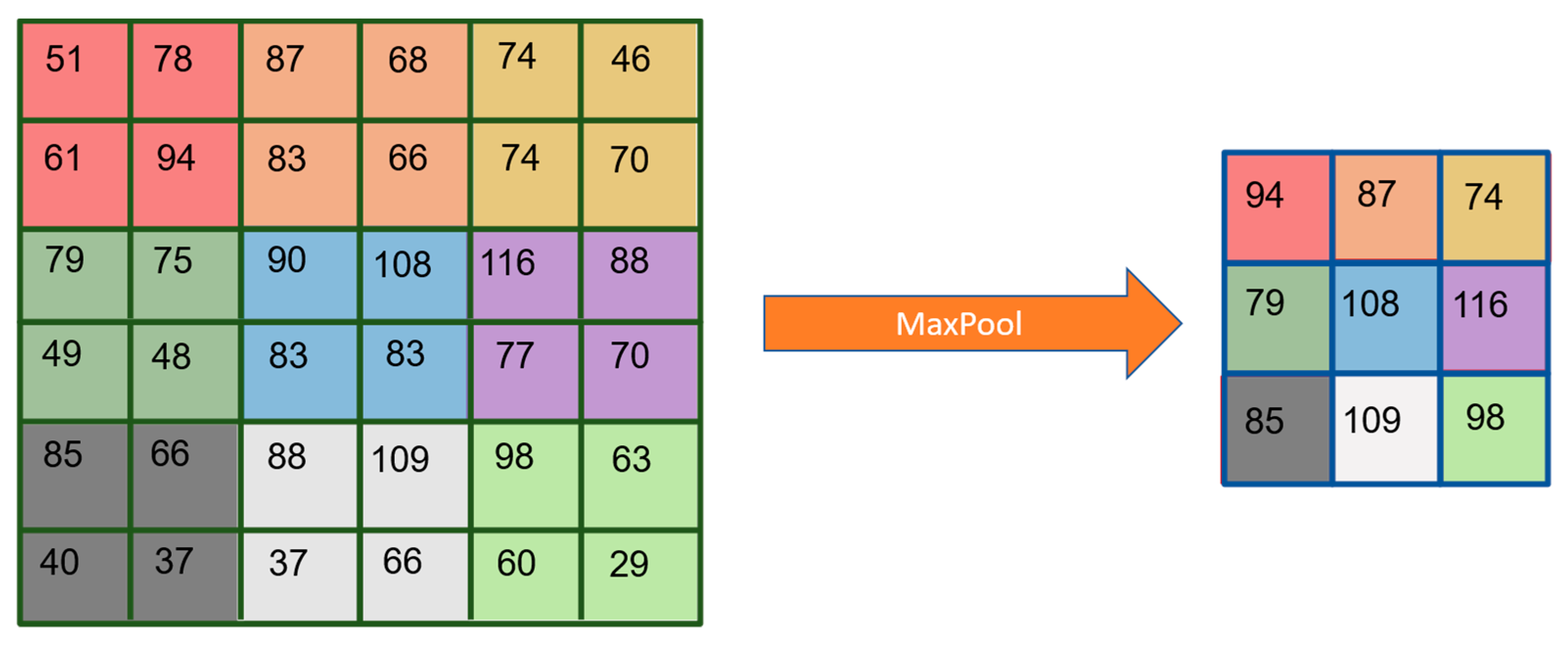
[22]Convolution via Sliding Filters (kernels)CNNOne-dimensional CNN (1D-CNN) based on vanilla architecture. The 1D-CNN model consists of two 1D convolutional layers, a max-pooling layer, and a fully connected layer followed by a SoftMax classifier and an output layer. A constant kernel size of 1 × 7 is applied to the convolutional layers.
[23]Hilbert Transformation, Discrete Wavelet Transformation, and DFTCNNThe paper is focused on voltage sags. There are three types of linked layers: convolution layers, pooling layers, and fully connected layers.
[24]Multiple Synchronous Reference Frame (MSRF) and Low-Pass FiltersLong Short-Term Memory (LSTM) and CNNThree methods are proposed: the first consists in the use of a low-pass Butterworth filter and a linear Finite Impulse Response (FIR)-based prediction. In the second method, the prediction is performed through an LSTM. Finally, in the third method, a deep convolutional neural network combined with an LSTM is used to filter and predict at the same time.
[25]-Explainable Artificial Intelligence (XAI)Four classifiers are considered, based on Rectified Linear Units (ReLU), max pooling layers, batch normalization layers, and CNNs with different kernel sizes.
Proposed Technique 1Discrete Fourier TransformationMLMVN3 layers, 50 Multivalued Neurons in the hidden layer, 6 Multivalued neurons in the output layer.
Proposed Technique 2Short-Time Fourier TransformationCNNCNN architecture with 6 layers of convolutions incrementing filter size on each layer and reducing the dimensionality using max pooling layers. The classification is conducted using a fully connected layer with 100 hidden layers and 6 outputs.
Table 3. Output Neurons and Fault Classes.
Fault ClassDescriptionOutput Combination
0No disturbances000000
1Voltage sag100000
2Voltage swell010000
3Harmonics distortion001000
4Voltage notch000100
5Interruption000001
Table 4. Training and Experimental Results for CNN.
Disturbance ClassTraining
CR%
Validation
CR%
0—Normal99.398.9
1—Sag100100
2—Swell100100
3—Harmonics100100
4—Notch100100
5—Interruption100100
Table 5. Recall Results for CNN.
Disturbance ClassTraining
CR%
Validation
CR%
0—Normal100100
1—Sag99.699.7
2—Swell99.799.2
3—Harmonics100100
4—Notch100100
5—Interruption100100
Table 6. Training Results for MLMVN.
Fault ClassTraining
CR%
Validation
CR%
0—Normal100100
1—Sag100100
2—Swell100100
3—Harmonics100100
4—Notch10099.19
5—Interruption100100
Table 7. Comparison with other classification methods.
Computational Intelligence TechniqueMain CharacteristicsTraining CR%Validation CR%
Convolutional Neural Network (CNN)In this case, a standard CNN is used to process time domain samples of the voltage waveforms. This is a neural network architecture that uses layers of convolution, pooling, and batch normalization for feature extraction. The convolutional layer is accompanied by a pooling layer, which is a type of downsampling that helps with processing speed. Basically, the CNN performs a convolution of the input signal with a kernel.89.2289.05
Feedforward Complex Neural NetworkIn this case, the three-layer feedforward architecture of a complex value network is used. Sampled waveforms are not processed before classification. Each sample in the time domain is considered to be the phase of a complex number with unit magnitude.80.9273.133
AlexNetAlexNet is a milestone in deep CNN and it is based on eight layers (five convolutional layers and three fully connected layers).
Support Vector MachineA quadratic SVM is used to directly process time domain samples of 8 kHz sampled voltage waveforms. A degree two polynomial kernel is used as the mapping function to make the samples separable. 89.1588.77
FFT + Support Vector MachineA quadratic SVM is used to process samples in the frequency domain. The same procedure explained above is followed. The voltage waveforms used for training are sampled at 8 kHz and then discrete Fourier transform is applied. The coefficients obtained are classified as real values by the SVM.9695.22
FFT + Decision TreeIn this case, the fine-tree algorithm of the MatLab classification learner library is applied on the coefficients of the discrete Fourier transformation.8483.3
Table 8. Classification Results with Different Time Intervals.
DisturbanceTime Interval
0.06 s0.6 s1 s2 s
1—Sag98.5%90%80%66.6%
2—Swell97%87.5%79.5%66.6%
3—Harmonics99.25%90%84%75%
4—Notch97%90%80%68%
5—Interruption98.5%90%80%70%
Disclaimer/Publisher’s Note: The statements, opinions and data contained in all publications are solely those of the individual author(s) and contributor(s) and not of MDPI and/or the editor(s). MDPI and/or the editor(s) disclaim responsibility for any injury to people or property resulting from any ideas, methods, instructions or products referred to in the content.

