Assessment of Power System Asset Dispatch under Different Local Energy Community Business Models

Abstract

Community energy projects have gained popularity in recent years, and encouraging citizens to form local energy communities (LEC) is considered an effective tool for raising awareness about renewable energy. Since no single universal method exists for operating LECs, this study investigated the impact that different business models and asset dispatch methods have on LECs’ economic and energy-related indicators. We carried out a case study, which included the development, modelling, and simulation of seven scenarios using mixed-integer linear programming (MILP). To measure and compare the prospective performance of the LECs in each scenario, six key metrics were evaluated and assessed. The authors find that simple, rule-based control systems might be well suited for LECs with a limited number of controllable assets that aim to provide increased levels of self-consumption of up to 3%. We also conclude that when the LEC utilises an energy cooperative business model, the selected asset dispatch method provides only minor differences in LEC performance, while for prosumer communities, the importance of selecting a suitable asset dispatch method is higher. We also conclude that LECs have the potential to significantly increase their economic performance by more than 10% by acting as aggregators and providing grid services directly to system operators.

1. Introduction

Increased penetration of renewable energy sources (RES) is changing the structure [1], planning [2] and modelling [3] of the energy system. In this context, flexibility [4] or power smoothing approaches [5] aim to address the technical challenges arising due to the difficult-to-control nature of electricity generation from local RES. On a higher level, various local energy generation and distribution solutions, such as local energy communities (LECs), need to be analysed as well, where additional challenges arise in the fields of the economic validity of the local system and the desire of consumers to get involved in the creation of such a system. One of the ways to overcome these challenges is to use LEC optimisation methods [6]—Economic Load Dispatch (ELD) optimisation associated with appropriate business models [7,8]. Several authors have addressed these two aspects very extensively.

Regarding ELD, the authors in [7] developed an algorithm for stochastic load scheduling for local energy systems, thus providing an opportunity to model the future load and generation structures and to carry out further planning and development measures. Other publications have addressed ELD modelling with various optimisation methods: Ref. [8] by using two-stage stochastic mixed-integer programming with cost, balance, and flexibility constraints, where the cost could be reduced by up to 5%, Ref. [9] by proposing dynamic ELD, including demand response activities, variable renewable energies and storage systems, but Ref. [10] describes ELD as isolated local energy system by using Particle Swarm Optimisation. When looking at business models, a review of the literature on energy communities in [11] gives insight into energy community business model structures, aspects, and pros and cons from the consumer perspective. Authors of [12] reviewed emerging energy community-related business models, strengths, and barriers to energy community development.

Although recent publications provide innovative solutions for ELD, as well as for the analysis of business models and the possibilities of their use in specific LEC layouts, a lack of connection between ELD and business models can be observed. There is a significant research gap on the impact of relevant business models on ELD optimisation measures and their results on social and economic welfare.

To fill this gap, this paper aims to determine the mutual influence of business models and ELD optimisation on LEC economic and energy-related indicators (self-consumption, self-sufficiency, levelized cost of energy and revenues). Furthermore, results of ELD optimisation for different business models are provided with the help of case studies.

The paper is organised as follows: Section 2 describes power system asset dispatch methods and provides an overview of LEC business models, Section 3 includes the description of the conducted case study and studied object, Section 4 provides a detailed description of the modelled and simulated scenarios, Section 5 includes the discussion, and Section 6 summarises relevant conclusions.

2. Power System Asset Dispatch and Energy Community Business Models

2.1. Power System Asset Dispatch

In this study, the ELD problem is extended to enable objectives aside from economic costs and to include different types of dispatchable power system assets (e.g., energy storage systems). Power system asset dispatch is considered a general minimisation problem with constraints and can be written in the following form:

min f(x), subject to g(x) = 0, h(x) ≤ 0,

(1)

where f(x) is the objective function, g(x) and h(x) are, respectively, the set of equality and inequality constraints, x is the vector of control and state variables [13]. There are general constraints applied in this study:

• The battery energy storage system (BESS) cannot charge and discharge simultaneously.
• The power balance equation is described as an equality constraint (2):

$$P_{pcc,out}+P_{BESS,c}+P_{Prosumer}=P_{pcc,in}+P_{BESS,d}+P_{PV,prod},$$

(2)

where $P_{pcc,out}$ is the active power exported from the LEC, $P_{BESS,c}$ the active power consumed by the BESS for battery charging, $P_{Prosumer}$ the aggregated active power consumption of all prosumers, $P_{pcc,in}$ the active power imported to the LEC, $P_{BESS,d}$ the active power produced during BESS discharging operation and $P_{PV,prod}$ the total active power produced by LEC photovoltaic generation plant (PV). However, there will always be some power loss, which is neglected by this equation.

The objective function varies based on the applied asset dispatch method. In this study, three different asset dispatch methods are investigated based on this general minimisation description:

• Maximisation of LEC self-consumption (LSC): If energy import from the grid can be minimised, the cost of buying additional energy is reduced. This minimisation of energy import means maximisation of self-consumption. For this minimisation method, the assets are shared equally in the community.
• Minimisation of levelized cost of energy (MLC): Shifting the import of energy to times with lower electricity prices reduces the cost of buying additional energy. Thus, this method’s minimisation goal is directly based on the imported electricity price instead of the electricity amount.
• Peer-to-peer energy trading (P2P): Like in the LSC method, minimising energy import to the LEC reduces the cost of buying additional energy. However, the P2P method considers the prosumers individually. There is a trading within the community where the prosumers try to reach their goals individually, maximising the energy matching within the community, which maximises self-consumption and minimises energy import.

2.2. Business Models Applied in Local Energy Communities

According to the authors of [14], new regulations and arrangements for electricity markets are necessary to encourage people to engage more in community initiatives and regional energy and power markets. Various business models may be applied in LECs. A comprehensive review of different LEC business models has been given in [12]. The following subsections give an overview of business models relevant to this study.

2.2.1. Energy Cooperatives (EC)

Energy cooperatives are one of Europe’s most common energy community types [15]. According to the European Federation of citizen energy cooperatives, over 1900 energy cooperatives across the European Union member states have at least 1.25 million active customers [16]. Energy cooperatives are created through citizen-led initiatives where end-users fund the installation of local generation systems [17], as shown in Figure 1. Energy cooperatives can be run with many different organisational forms and financing models. Some are run as companies with profit-making in mind, where the shareholders finance medium to large-scale PV or wind power plants. Others can be non-profit organisations that finance local production of renewables to cover the self-consumption and the sale of surplus [18].

Energy cooperatives may be given the right to act as a sort of local distribution system operator (DSO) responsible for managing their low-voltage network. This operation enables them to exempt cooperative members from some of the use-of-system tariffs while incentivising self-consumption through dynamic pricing schemes and other billing conditions [19]. The roles that energy cooperatives may take are not standardised on the European legislative level and, thus, may depend on the regulations and network codes from country to country. For example, in Portugal, energy communities may be allowed to take over the responsibility of the DSO for the local community grid, while in the Netherlands, it is explicitly forbidden [20].

2.2.2. Prosumer Communities (PC)

Energy prosumer communities are often established by prosumers acting as decision-makers, investors, and customers. They cooperate to take advantage of favourable financing circumstances when buying assets in bulk and to acquire dimension for participation in flexibility markets, benefiting from collective energy efficiency (EE) initiatives or participating in local energy markets (LEM) [12]. In contrast to energy cooperatives, where end-users cooperate in acquiring medium to large-scale on-site generation, the prosumer community business model consists of individual small-scale prosumers in local communities, as depicted in Figure 2. These prosumers can act as decision-makers, investors, and customers. The source of revenue comes from trading their flexibility on LEMs, EE initiatives, and participation in flexibility markets [19]. Residents of the community sign a long-term public purchase agreement (PPA) with energy providers to sell the excess generation and purchase the leftover deficit energy. Members of the community can also trade energy among themselves (LEM or P2P trading), which relieves them of the obligation to pay fees associated with medium- and high-voltage distribution and transmission networks outside of their own grid [21].

An example of community prosumerism includes the city of Litoměřice in the Czech Republic, where the local municipality and households financed a project that involved installing PV systems and energy efficiency measures to reduce the community’s energy consumption from the main grid [12].

Prosumers are individuals who generate, utilise, and modulate their own renewable energy [19]. They include residential, commercial, and industrial entities [19]. The difficulties faced by energy systems are widely perceived as being resolved through prosumerism. In the light of this, the implementation of distributed energy systems (DES), in which energy is generated and consumed locally, is led by prosumers, lowering greenhouse gas emissions and assuring local value creation.

The advantages of energy “autarky” are emphasised by proponents, where various energy vectors, such as electricity, heating, transportation, and valuable work, may be obtained locally from sources such as solar, wind, geothermal, waste, and biogenic sources in increasingly closed-loop, circular systems. As a way to counteract the erratic nature of renewable energy sources, these scenarios also include demand-side behavioural changes such as storage and flexibility service offering and time-of-use (TOU) prices.

The necessity of new business models has been emphasised by several authors as a means of easing the transition to decentralized and prosumer-driven energy systems. These models may make it easier for people to use more renewable energy on their own, trade electricity locally, maintain the stability of the grid, and switch to other energy sources for heating and transportation. Limited number of studies have highlighted the various forms of value that such business models may produce as well as how they may be managed [22].

As per Ref. [23], the energy prosumer comprises two entities: the prosumer subject and its resources. The prosumer subject can be described as an owned who is proactive or its delegated manager (autonomous agent). The prosumer subject is responsible for formulating its strategic goals, e.g., emphasise renewable energy rather than minimise energy cost. The prosumer subject comprises of a well-informed agent, prosumer objectives, and requirements, and the prosumer assets are its financial assets, goods, and technology system.

Asset dispatch in CP energy communities can be performed with the following methods:

• Peer-to-peer energy trading;
• Maximising self-consumption;
• Minimising levelized cost of energy.

2.2.3. Community Flexibility Aggregation (CFA)

Due to its limited size and lack of flexibility, a single household does not offer sufficient flexibility for any significant grid enhancement and may find it difficult to engage in markets. When prosumers join, additional value may be created by aggregating their demand, supply, and energy flexibility. Thus, aggregation allows the prosumers to combine their resources, which allows them to gain more substantial leverage in negotiations with retailers and last-resort traders.

In addition to on-site RES, residential prosumers can find value in the intelligent management of smart appliances. These devices can broadly be divided into three categories [24]. Thermostatically controlled loads (TCLs) include space heating systems with smart thermostats and domestic water heaters (DHW). TCLs can be controlled within specific temperature ranges according to the prosumer’s comfort requirements [25]. Shiftable appliances include wet appliances such as dishwashers, clothes washing machines, and drying machines. The usage of these devices can be shifted when there is a surplus of PV power or a cheaper electricity price. Storage devices such as battery systems can store surplus energy as electricity for later usage. In future electricity grids, electric vehicles (EVs) constitute a large share of local community energy demand that could be intelligently controlled. In the case of vehicle-to-grid (V2G) technology, the EVs can also provide bidirectional energy flow support and be considered a sort of mobile battery system [26].

The aggregation of residential community flexibility has many benefits. However, the real-world implementation would require consent from all aggregation participants and citizens might not have the technical skills or resources to implement this. In addition, cyber-physical infrastructure would become vital to facilitate the proper activation of devices and logging information related to billing purposes. Other aggregation challenges include legislative hindrances, such as the lack of clearly defined roles of the participant and the lack of definitions of flexibility services [27].

Communities formed with the purpose of aggregating power system flexibility aim to use demand side management (DSM) incentives to collectively and directly participate in flexibility services procured by system operators. CFA can also be realised through an aggregator that pools demand flexibility to reach sufficient volumes to make offers in reserve, balancing, or ancillary markets [28] or to an electricity retailer to balance its portfolio to avoid deviation penalties [29]. Residential demand flexibility is likely to become more appealing to businesses thanks to energy communities [30], while the author of [31] states that residential demand flexibility has already become economically feasible for LECs.

Compared with PC, the CFA business model does not expect all members to include energy production, as shown in Figure 3. Thus, their uptake is considered less costly and with lower complexity, meaning the technological infrastructure for such communities is easier to establish. For CFA-based LECs that are made up of residential dwellings, the flexibility pool consists of larger electricity consumers, e.g., heat pumps, electric vehicle (EV) chargers, and air conditioning (AC) units. The initiative for forming these communities might stem from aggregators [12] or property developers. A key enabler for forming such systems is the uptake of consumer devices that feature built-in functionality to participate in DSM incentives, e.g., OpenADR certified products [32], which reduce the integration cost of flexible loads.

LEC business models require different approaches for solving asset dispatch. A mapping of analysed asset dispatch methods that apply to more common LEC business models is provided in

Table 1. Asset dispatch methods that apply to different LEC business models.

LEC Business Model	P2P	LSC	MLC
EC		✔	✔
PC	✔	✔	✔
CFA			✔

.

A case study is carried out to understand the economic performance of different asset dispatch methods under different business models.

3. Case Study and Object Description

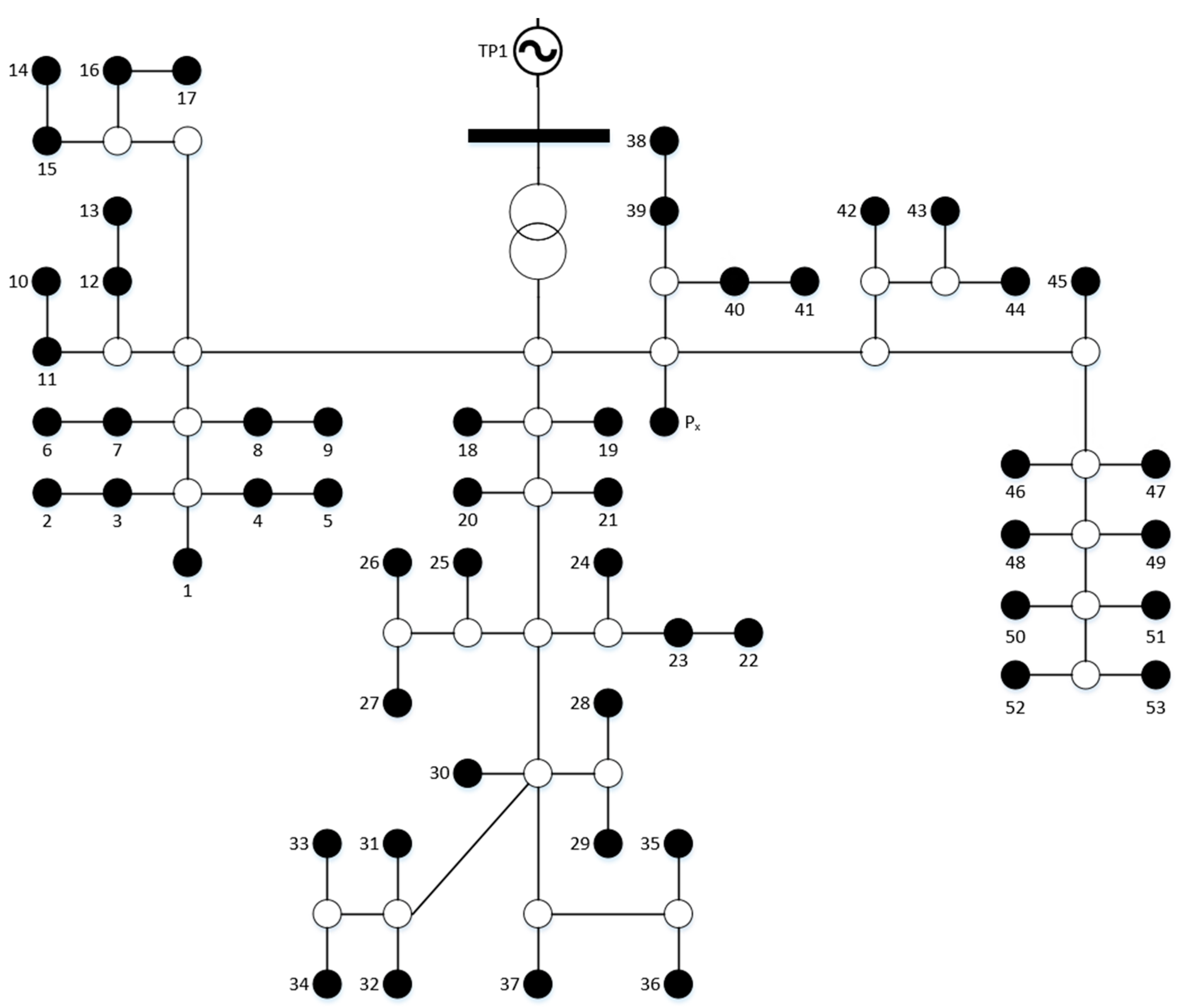
Six scenarios are studied corresponding to the combinations of LEC business models and asset dispatch methods (Table 1). A benchmark simulation, which incorporates asset dispatch in the form of a robust rule-based controller for controlling a BESS, is also carried out for comparison. The topology of an actual segment of an electricity distribution system of a residential area in Riga is used. 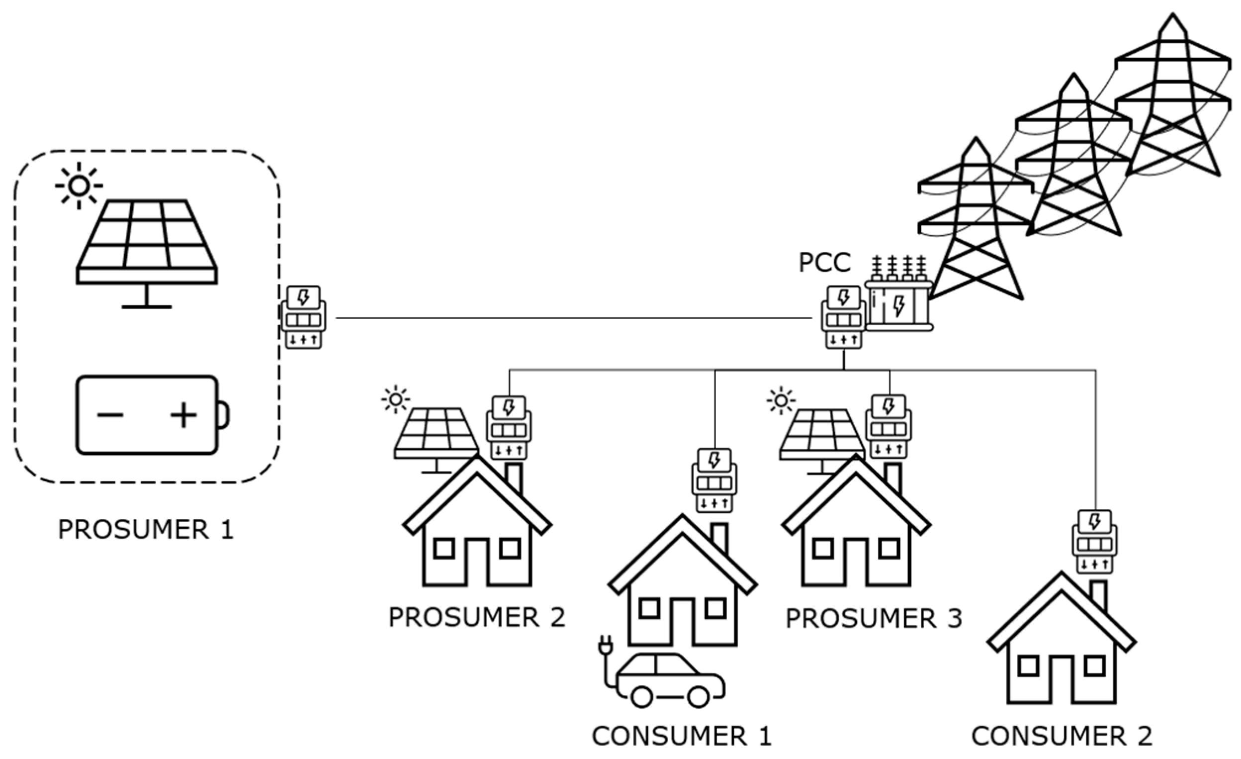The generalised topology of the electric power system is depicted in Figure 4. To prevent possible breaches of privacy, the metering data used in the study is not collected from the same system. Instead, residential consumers and PV production plants’ individually collected and anonymised metering data is mapped to the LEC power system nodes. The dataset used for the study has a time step of 1 h and a range of 3 years. The distribution grid used in the case study includes one common grid connection point (point of common coupling—PCC) and 53 nodes, from which 38 are plain consumers, and 15 are prosumers.

Additionally, a generic prosumer (denoted as P_x) is included in the system. The generic prosumer incorporates a larger (rated at 50 kW) PV production unit and a grid-scale BESS (rated at 75 kW, 200 kWh). The ownership and operation of prosumer P_x vary between different scenarios.

Based on the collected data, a set of control and state variables is synthesised for each consumer and prosumer node. A summary of the connection capacity and available flexibility for each node is provided in

Table 2. A general summary of control and state variables for LEC nodes used in the case study.

Node	Connection Capacity (kW)	Flexibility (kWh)	Node	Connection Capacity (kW)	Flexibility (kWh)	Node	Connection Capacity (kW)	Flexibility (kWh)
1	11	0.2	19	11.0	0.2	37	11.0	1.3
2	11	0.0	20	21.0	1.8	38	13.0	0.0
3	11	0.6	21	11.0	0.8	39	13.0	0.8
4	11	0.0	22	11.0	0.5	40	13.0	1.3
5	11	0.0	23	11.0	0.2	41	11.0	0.5
6	11	0.0	24	11.0	0.0	42	11.0	0.5
7	11	0.0	25	13.0	0.0	43	21.0	1.3
8	11	0.2	26	11.0	0.2	44	11.0	1.1
9	11	0.2	27	11.0	0.5	45	26.0	4.5
10	16	1.6	28	16.0	2.5	46	11.0	0.0
11	16	0.6	29	16.0	1.6	47	11.0	0.5
12	11	0.0	30	11.0	0.2	48	11.0	0.0
13	11	0.2	31	11.0	0.2	49	11.0	1.3
14	16	0.5	32	11.0	0.0	50	11.0	0.5
15	16	0.8	33	11.0	0.6	51	11.0	0.8
16	16	4.5	34	11.0	0.0	52	13.0	0.0
17	16	3.1	35	11.0	0.5	53	13.0	0.8
18	16	1.6	36	11.0	0.6	Px	75.0	160.0

. We use a simplified approach to incorporate power system flexibility. The following estimations and simplifications are applied:

• Each prosumer node is characterised by the amount of flexibility it has available (Table 2), which should be treated as synthesized sample values;
• Since the timestep of the simulation is 1 h, the flexibility is described as available energy;
• Each prosumer can provide up or down-regulation with a duration of 1 h;
• For up-regulation (decreasing output energy), for each prosumer, the rebound is considered with a duration of 2 h, during which a total of 30% more energy is consumed than what was used for flexibility activation;
• For down-regulation (increasing output energy), for each prosumer, the rebound is considered with a duration of 2 h, during which a total of 30% less energy is consumed than what was used for flexibility activation;
• Flexibility activation in both directions is always available for each prosumer, except during rebound.

A more accurate presentation of prosumer flexibility and its activation, including data about actual system requirements for purchasing flexibility, is in the scope of future research. For the utilisation of flexibility, a set of state space variables was generated, which is used to indicate how much of the magnitude can be utilised for each specific time-space. The control variables remain the same throughout all studied scenarios.

Mixed-integer linear programming (MILP) is used to evaluate the different scenarios. For the six scenarios, a deterministic setup is created using a one-year segment of the input data, PV production data for the year 2018 acquired from the EU Science Hub using the PVGIS Online tool [33] and Nord Pool Spot Market prices for years 2021 and 2022 [34].

The simulations aim to evaluate the differences between the potential of LECs that operate with different business logic and utilise different methods for asset dispatch. Six key indicators are used to assess LEC performance: self-consumption, self-sufficiency, levelized cost of energy (LCOE), import cost, export revenue and revenue from monetising available power system flexibility.

The self-consumption, denoted as $SC$, is calculated by Equation (3) as the ratio of PV generation used on-site to the total PV production.

$$SC=\frac{\sum produced PV energy-\sum exported pv energy}{\sum produced PV energy}.$$

(3)

The self-sufficiency of the LEC, denoted as $SS$, is considered as the share of prosumer demand, which is covered by on-site generation and is calculated using Equation (4).

$$SS=\frac{\sum E_{prosumer}-\sum E_{PCC,imp}}{\sum E_{prosumer}}.$$

(4)

In a general form, the LCOE can be defined as:

$$LCOE=\frac{sum of costs over lifetime}{sum of energy produced over lifetime,}$$

(5)

but this definition is typically applied to generation units only. In the concept of this work, the focus is on the LCOE for an entire LEC, which means Equation (5) is adapted separately for each investigated scenario. A detailed description of the calculation of the LCOE is provided with the description of each scenario. The cost of importing energy is calculated by Equation (6).

$$C_{import}=E_{Pcc,imp}·\left(p_e+tariff\right),$$

(6)

where $E_{Pcc,imp}$ denotes the energy imported through the PCC, $p_e$ is the price of energy at the Nord Pool Spot Market and $tariff$ the summarised capacity-based value for system operator tariffs and taxes specific to the environment. Nord Pool Spot Market prices for the year 2021 for Estonia (EE) market region are used. The case study uses a simplified approach for considering grid tariffs and relevant taxes, where a constant value of 0.025 €/kWh is used throughout the study. The energy export revenue is considered a negative cost and is calculated using Equation (7).

$$C_{export}=E_{Pcc,exp}·p_e,$$

(7)

where $E_{Pcc,exp}$ denotes the energy exported through the PCC. Based on the existing tariff structure of Estonia, energy export is not taxed with grid tariffs and respective taxes. We use a simplified approach for assessing the value generated through flexibility incentives to manage the complexity of this work. We have purposely simplified the commonly applied method for incentivising flexibility, where the generated revenue comprises two components: separate remuneration for availability and activation. This study calculates the revenue generated through flexibility incentives using Equation (8).

$$C_{prosmer,flex}=p_{flex}·E_{prosumer,flex,}$$

(8)

where $p_{flex}$ denotes the price of flexibility activation and $E_{prosumer,flex}$ the energy used for flexibility activation. We have neglected input data about actual flexibility activations from the grid, and in this study, we use a simplified notion that the grid is willing to purchase flexibility activation at each time step. Improving the modelling of flexibility remuneration and considering actual activations is the subject of future work. Following is a detailed description of each scenario.

4. Modelling and Simulation of Optimisation Scenarios

The following subsections present the formulation of the optimisation problems. Let the set of time horizons be $\mathcal{H}=\{\mathrm{1,2},\dots H\}$, where $H$ is the length of the optimisation horizon and $t$ the index of the time step. Let the set of prosumers be $\wp =\{\mathrm{1,2},\dots ,53\}$, where the index of a prosumer is $j$. To manage computational requirements, the optimisation is performed with a 1-week time horizon, and all weeks of the year are simulated sequentially, with the results of the previous weeks used as input for the subsequent simulations. Optimisations for scenarios 1 to 5 are performed in this manner. The last, 6th scenario uses a 1-day horizon, and all scenarios utilise a 1h timestep.

4.1. Benchmark Scenario

A rule-based controller for the PV and BESS of P_x was developed to provide a comparative benchmark. The operational algorithm for controlling the BESS in the benchmark scenario is presented in Figure A1 (Appendix B). The control of the BESS in the benchmark scenario is based on energy flows through the PCC and the BESS’s state of charge (SOC). The control is implemented such that the BESS aims to maximise self consumption. If the local generation produces more energy than is consumed by the LEC loads, excess energy is stored in the BESS until the SOC reaches 100%, upon which the excess energy is exported to the grid. However, if the local generation is not sufficient to cover LEC demand, the BESS is discharged to cover the deficit until the SOC drops to 20%, upon which the deficit is covered by importing energy from the grid. The equations below are used to determine the SOC of the BESS:

$$E_{BESS}\left(t\right)=E_{BESS}\left(t-1\right)+{\mu }_c{E}_{BESS,c}\left(t\right)-\frac{E_{BESS,d}\left(t\right)}{{\mu }_d},$$

(9)

$$\mathrm{S}\mathrm{O}\mathrm{C}\left(t\right)=\frac{E_{BESS}\left(t\right)}{E_{BESS,max}},$$

(10)

where $E_{BESS}$ denotes the energy stored in the battery, $E_{BESS,c}$ the energy consumed by the BESS during charging, $E_{BESS,c}$ the energy produced by the BESS during discharging, ${\mu }_c$ charging efficiency and ${\mu }_d$ the discharging efficiency; $SOC$ denotes the battery state of charge and $E_{BESS,max}$ describes the nominal capacity of the battery. The developed algorithm is designed to prohibit energy arbitrage by the BESS, and only excess PV energy can be exported through the PCC to the grid. Thus, Equation (3) can be reformulated as:

$$SC=\frac{\sum E_{PV}\left(t\right)-\sum E_{Pcc,exp}\left(t\right)}{\sum E_{PV}\left(t\right)}.$$

(11)

The LCOE for the benchmark scenario is calculated using Equation (12).

$$\mathrm{L}\mathrm{C}\mathrm{O}\mathrm{E}=\frac{C_{inv}+C_{maint}+C_{import}-C_{export}}{\sum P_{prosumer}},$$

(12)

where, $C_{inv}$, $C_{maint}$, stand for the cost of investment and maintenance of the PV and BESS systems, respectively. The PV’s investment cost is 556.99 €/kWp with a maintenance cost of 5.57 €/kWp per year [15]. The investment cost of the BESS is 1876.00 €/kW + 469.00 €/kWh, with a maintenance cost of 10.00 €/kW per year [13].

The results of the benchmark scenario indicate that the LEC has a high self-consumption rate of 92.9%. The self-sufficiency of the LEC was 25.2%, while the LCOE was calculated to be 0.134 €/kWh. The accumulated cost of importing energy for one year was 51,404 €, and the revenue from selling energy to the grid was 640 €. The total operation cost (the import less the export and flexibility revenues) was 50,764 € for the simulation period (1 year). To compare the performance of different scenarios, the results of all simulations are compiled in

Table 3. Summary of simulation results with 2021 Nord Pool Spot Prices.

Parameter	Benchmark	EC+LSC	EC+MLC	PC+P2P	PC+LSC	PC+MLC	CFA+MLC
Self-consumption [%]	92.86	92.77	92.02	92.77	92.87	91.03	85.35
Self-sufficiency [%]	25.20	25.01	24.79	28.25	25.18	25.23	24.10
LCOE [€/kWh]	0.1338	0.1338	0.1329	0.1278	0.1328	0.1307	0.1192
Import cost [€]	51,404	51,478	51,165	51,522	51,082	48,665	47,085
Export revenue [€]	640	691	902	690	686	1043	2941
Flexibility revenue [€]	-	-	-	-	466	581	3682
Total operation cost [€]	50,764	50,787	50,263	50,832	49,930	47,041	40,462

.

4.2. Scenario 1: LEC as Energy Cooperative to Maximise Self-Consumption (EC+LSC)

In this scenario, the LEC is formed as an Energy Cooperative, where all 53 prosumers are equal members, and the assets of P_x are treated as community owned, where all profits and losses are shared among community members. The goal of the LEC is to maximise self-consumption, while the power output of the BESS is the only manipulated variable.

For this scenario, the optimisation variables include the charging and discharging energies of the BESS ($E_{BESS,c}$ and $E_{BESS,d}$), the energy output of the BESS ($E_{BESS}$), and the imported and exported energy through the PCC ($E_{Pcc,imp}$ and $E_{Pcc,exp}$). The maximisation of self-consumption of the LEC can be defined as maximising the share of locally produced energy that is consumed locally. In scenario 1, only the energy produced by the local PV systems can be exported. Thus the objective function can be formulated as to minimise the exported energy:

$$\min {\mathit{E}}_{\mathit{Pcc},\mathit{exp}}={\sum }_{t=1}^H{E}_{Pcc,exp}\left(t\right).$$

(13)

The optimisation task in this scenario is subject to different constraints. The defined BESS has a capacity of 200 kWh, with a minimum SOC value of 20%.

$$40 \mathrm{k}\mathrm{W}\mathrm{h}\le {SoC}_{BESS}\left(t\right)\le 200 \mathrm{k}\mathrm{W}\mathrm{h}.$$

(14)

The energy state evolution of the BESS can be described by an equality constraint Equation (15). The BESS is assumed to start the first timestep in a depleted state of 20% SOC.

$${\mathrm{S}\mathrm{O}\mathrm{C}}_{BESS}\left(t\right)={\mathrm{S}\mathrm{O}\mathrm{C}}_{BESS}\left(t-1\right)+E_{BESS,c}\left(t\right)·{\mu }_c-\frac{E_{BESS,d}\left(t\right)}{{\mu }_d}.$$

(15)

The charging power of the BESS is limited by inequality constraints Equation (16), Equations (17) and (18), where $E_{BESS,c,max}$ and $E_{BESS,d,max}$ denote the maximum allowed charging and discharging power of the BESS (75 kW), which is considered the maximum amount of energy the BESS can absorb or release in 1 h. Additional auxiliary binary variables ${\zeta }_c$ and ${\zeta }_d$ are introduced to forbid simultaneous charging and discharging.

$$0\le E_{BESS,c}\le E_{BESS,c,max}·{\zeta }_c,$$

(16)

$$0\le E_{BESS,d}\le E_{BESS,d,max}·{\zeta }_d,$$

(17)

$${\zeta }_c+{\zeta }_d\le 1,$$

(18)

Even though the throughput limit of the PCC is not considered in this work, the constraints Equations (19)–(21) were implemented to forbid the simultaneous import and export through the PCC using auxiliary binary variables ${\zeta }_{in}$ and ${\zeta }_{out}$. A large constant of 10 MWh was used as an energy limit.

$$0\le E_{Pcc,imp}\le \mathrm{10,000}·{\zeta }_{in},$$

(19)

$$0\le E_{Pcc,exp}\le \mathrm{10,000}·{\zeta }_{out},$$

(20)

$${\zeta }_{in}+{\zeta }_{out}\le 1,$$

(21)

In this scenario, the idea was to entirely utilise the locally produced PV power. Thus additional constraints Equations (22) and (23) were implemented to forbid energy arbitrage through charging and discharging the BESS from and to the grid.

$${\zeta }_d+{\zeta }_{out}\le 1,$$

(22)

$${\zeta }_c+{\zeta }_{in}\le 1,$$

(23)

An energy balance constraint Equation (24) was included to ensure that there would be a balance between the produced/imported energy and consumed/exported energy. The demand of prosumers is denoted with $E_{prosumer}$ and the combined PV production of grid-scale PV and the prosumer PV-s is given with $E_{PV}$.

$$E_{Pcc,exp}+E_{BESS,c}+E_{prosumer}=E_{Pcc,imp}+E_{BESS,d}+E_{PV},$$

(24)

The LCOE for this scenario is calculated using Equation (12), the same as for the benchmark scenario. The results of the EC+LSC scenario show that maximising the self-consumption resulted in 92.8% of PV energy being consumed locally (self-consumption), while the self-sufficiency of the LEC was 25.0%. The levelized cost of energy was 0.134 €/kWh, while the accumulated cost for importing energy for one year was 51,478 €, revenue from selling to the grid 691 €, and total operation cost 50,787 €.

4.3. Scenario 2: LEC as Energy Cooperative to Minimise Levelized Cost of Energy (EC+MLC)

The second scenario uses the same Energy Cooperative business model utilised in the EC+LSC scenario but minimises the LCOE. Like the previous scenario, the only manipulated variable is the power output of the BESS, but the optimisation includes a price component. The algorithm attempts to shift the discharging of the battery to times of high electricity price to lower the cost of consumed energy. The optimisation variables and constraints remain the same as used in the EC+LSC scenario, while the optimisation objective is subject to change. The LCOE for this scenario is calculated using Equation (12), the same as for the benchmark scenario. The only influenceable parts of the LCOE equation are energy import and export cost components. Therefore, the optimisation objective of this scenario can be formulated as Equation (25).

$$\min \mathrm{LCOE}={\sum }_{t=1}^H{C}_{import}\left(t\right)-C_{export}\left(t\right)$$

(25)

where $C_{import}$ denotes the cost of imported energy and $C_{export}$ the revenue of exported energy (presented as negative cost).

The results of the EC+MLC scenario show that the maximisation of LCOE resulted in 92.0% self-consumption and 24.8% self-sufficiency. The LCOE of the LEC was 0.133 €/kWh, while the accumulated cost for importing energy for one year was 51,165 €, the revenue from PV energy export 902 €, and the total operation cost 50,832 €.

4.4. Scenario 3: LEC as Prosumer Community to Facilitate Peer-to-Peer Trading (PC+P2P)

The third scenario uses peer-to-peer (P2P) trading in a prosumer community. The LEC comprises 54 prosumers (all 53 prosumer nodes and the node denoted as P_x), which have formed a community to facilitate intra-community P2P trading. All prosumers are assumed to act selfishly to meet their individual goals. In this scenario, the demand flexibility of prosumers and consumers is also considered. The flexibility is monetised through an abstract aggregator which resides outside of the LEC and remunerates flexibility activation with a constant $p_{flex}$ value of 0.01 €/kWh. The objective in this scenario is to maximise the matched energy production with consumption within the LEC. This objective is based on the hypothesis that matching energy inside the LEC increases economic feasibility since energy import is reduced. Thus, the cost of grid tariff is lower.

Additional optimisation variables need to be incorporated into the optimisation due to the inclusion of prosumer flexibility. The flexibility-aware prosumer load is denoted as $E_{prosumer,flex}$. The prosumer flexibility activations are considered with a binary variable $Pro{s}_{flex}$. Two binary variables are declared to represent the state of rebound for each of the rebound hours, $Reboun{d}_1$ and $Reboun{d}_2$. Additional constraints need to be included in the addition of prosumer flexibility. The flexibility and rebound aware load of prosumers can be formulated with Equation (26).

$$E_{prosumer,flex}\left(j,t\right)=E_{prosumer}\left(j,t\right)+E_{Flex}\left(j\right)·Pro{s}_{flex}\left(j,t\right)-E_{rebound}\left(j\right)·Reboun{d}_1\left(j,t\right)-E_{rebound}\left(j\right)·Reboun{d}_2(j,t),$$

(26)

where $E_{Flex}\left(j\right)$ and $E_{rebound}\left(j\right)$ are the energies of activated flexibility and their subsequent rebound (as shown in Table 2 and described in Section 3). To prevent the activation of flexibility from resulting in negative demand for the prosumers, the following constraint is included:

$$E_{prosumer,flex}(j,t)\ge 0,$$

(27)

The rebound activation must happen directly in the subsequent timesteps of the flexibility activation. Therefore constraints Equations (28) and (29) are included. It is assumed that there is no rebound event in the first 2 h of the simulation year.

$$Reboun{d}_1\left(j,t+1\right)=Pro{s}_{flex}(j,t),$$

(28)

$$Reboun{d}_2\left(j,t+1\right)=Pro{s}_{flex}(j,t),$$

(29)

Due to the nature of a weekly optimisation horizon, it is assumed that the flexibility cannot be activated during the last 2 h of each week. This is because the optimisation algorithm is unaware of the demand of prosumers and the PV production of next week. Therefore, activating flexibility on the final 2 timesteps could result in an unfeasible solution for the next week. Flexibility activation during the rebound process is prevented with constraints Equations (30) and (31).

$$-1\le Pro{s}_{flex}(j,t)+Reboun{d}_1(j,t)\le 1,$$

(30)

$$-1\le Pro{s}_{flex}\left(j,t\right)+Reboun{d}_2(j,t)\le 1,$$

(31)

The energy balance constraint used in previous scenarios was modified to include the flexibility and rebound-aware prosumer load. The resulting constraint is formulated by Equation (32).

$$E_{Pcc,exp}+E_{BESS,c}+E_{prosumer,flex}=E_{Pcc,imp}+E_{BESS,d}+E_{PV},$$

(32)

In P2P trading, the goal is to maximise the matched energy production and consumption within the LEC. This is implemented using Equation (33), where the optimisation goal is to minimise the absolute difference between imported and exported energy through the PCC.

$$\min E_{\mathit{Pcc},\mathit{dif}}=\left({\sum }_{t=1}^H\left|E_{Pcc,imp}\left(t\right)+E_{Pcc,exp}\left(t\right)\right|\right),$$

(33)

The LCOE for this scenario is calculated using Equation (12), the same as for the benchmark scenario. The results of the PC+P2P scenario show that maximising the self-consumption resulted in self-consumption of 92.8% and self-sufficiency of 28.3%. The LCOE energy was 0.128 €/kWh, while the accumulated cost for importing energy for one year was 51,522 €, the revenue from selling to the grid 690 €, and the total operation cost 50,832 €.

4.5. Scenario 4: LEC as Prosumer Community to Maximise Self-Consumption (PC+LSC)

Like the EC+LSC scenario, this scenario aims to maximise the LEC’s self-consumption, using the Prosumer Community business model described in the PC+P2P scenario. Since prosumers are assumed to act selfishly, they all attempt to maximise their individual self-consumption. The prosumers do this by timing their consumption to coincide with the period when PV is produced though their energy flexibility. The energy flexibility of consumers is not considered since they have no on-site generation to shift their demand. The prosumer P_x is considered different and aims to maximise the self-consumption of the entire LEC.

The simulation is performed in two steps: first, the operation of every prosumer is optimised individually; second, the operation of P_x is optimised using the results from the first step. For the second step, the optimisation variables and constraints remain the same as for the PC+P2P scenario. For the first step, the only difference is the energy balance constraint Equation (34), which does not include the BESS component.

$$E_{Pcc,exp}+E_{prosumer,flex}=E_{Pcc,imp}+E_{PV,prosumer}.$$

(34)

The optimisation goal Equation (35) remains the same as for the EC+LSC scenario, which also aims to maximise LEC self-consumption. However, it is used separately for each prosumer.

$$\min E_{Prosumer,exp}={\sum }_{t=1}^H{E}_{Pcc,exp}\left(t\right).$$

(35)

The calculation of the LCOE for comparing LEC performance includes the flexibility component Equation (8), which incentivises prosumers to use their flexibility.

$$\mathrm{L}\mathrm{C}\mathrm{O}\mathrm{E}=\frac{C_{inv}+C_{maint}+C_{import}-C_{flex}-C_{export}}{\sum E_{prosumer}},$$

(36)

The results of the EC+LSC scenario show that maximising the self-consumption in a Prosumer Community resulted in self-consumption of 92.9% and self-sufficiency of 25.2%. The LCOE energy was 0.133 €/kWh, while the accumulated cost for importing energy for one year was 51,082 €, and the revenue from selling to the grid was 686 €. The revenue generated by providing flexibility was 466 €, and the total operation cost was 49,930 €.

4.6. Scenario 5: LEC as Prosumer Community to Minimise Levelized Cost of Energy (PC+MLC)

This scenario is like the EC+MLC scenario that attempts to minimise the LCOE of the LEC. However, in this scenario, the optimisation is carried out for a Prosumer Community described in the PC+P2P scenario. For this case, the prosumers are assumed to minimise their individual LCOE. Like the EC+LSC scenario, the optimisation is performed in two steps: first, for the 53 prosumer nodes, and second, for the prosumer P_x. Compared to the EC+LSC scenario, new optimisation variables are included that describe the flexible energy of the prosumers: $E_{prosumer,flex,up}$ and $E_{prosumer,flex,down},$. The objective function Equation (37) is extended from the EC+MLC scenario to include the component of revenue generated from flexibility Equation (38), and it is applied to individual prosumers.

$$\min {\mathrm{L}\mathrm{C}\mathrm{O}\mathrm{E}}_{Prosumer}={\sum }_{t=1}^H{C}_{import}\left(t\right)-C_{export}\left(t\right)-C_{prosumer,flex}$$

(37)

$$C_{prosumer,flex}=E_{prosumer,flex,down}·p_{flex}-E_{prosumer,flex,up}·p_{flex},$$

(38)

The goal of the prosumer P_x is still to minimise the LCOE of the entire LEC using the objective function Equation (25) described in the EC+MLC scenario.

The results of the PC+MLC scenario show that minimising the LCOE in a Prosumer Community resulted in self-consumption of 91.0% and self-sufficiency of 25.2%. The LCOE energy was 0.131 €/kWh, while the accumulated cost for importing energy for one year was 48,665 €, and the revenue from selling to the grid was 1043 €. The revenue generated by providing flexibility was 581 €, and the total operation cost was 47,041 €.

4.7. Scenario 6: LEC as Collective Flexibility Aggregation to Minimise Levelized Cost of Energy (CFA+MLC)

The final scenario considers a LEC which operates under a Collective Flexibility Aggregation business model. In this scenario, the flexibility of the 53 prosumer nodes and the prosumer P_x is controlled by an aggregator, which resides inside the LEC. We consider a hypothetical setup where the DSO procures flexibility (up- and downregulation) with a step of 100 kW in 1 h blocks. To paraphrase it, the LEC operates as an aggregator and provides flexibility directly to the DSO. The activation of flexibility is rewarded with a constant $p_{flex}$ value of 0.02 €/kWh. The remuneration of flexibility is double than considered in the PC+LSC and PC+MLC scenarios since there is no aggregator between the LEC and the system operator. The LEC aims to minimise its LCOE. Due to the computational requirements of this scenario, the optimisations are performed within a 1-day time horizon.

The previously used optimisation variables for prosumers were decoupled to represent the direction of energy flow: $pro{s}_{flex,up}$, $pro{s}_{flex,down}$, $reboun{d}_{1,up}$, $reboun{d}_{2,up}$, $reboun{d}_{1,down}$, and $reboun{d}_{2,down}$. Additionally, new optimisation variables were included in determining the binary activation of aggregated flexibility ($AG{G}_{flex,up}$ and $AG{G}_{flex,down}$) and the rebound of aggregated flexibility ($AG{G}_{reb,up,1}$, $AG{G}_{reb,up,2}$, $AG{G}_{reb,down,1}$ and $AG{G}_{reb,down,2}$). The energy of the BESS of P_x was decoupled into energy used during the period when no flexibility was activated ($E_{BESS,c}$ and $E_{BESS,d}$) and the period when flexibility was used ($E_{BESS,flex,c}$ and $E_{BESS,flex,d}$). The energy of aggregated flexibility was denoted as ($AG{G}_{flex,pwr,up}$ and $AG{G}_{flex,pwr,down}$).

Additional constraints Equations (39) and (40) were included for the aggregated control to ensure the flexibility of prosumers is only activated during aggregation.

$$pro{s}_{flex,up}\left(j,t\right)\le AG{G}_{flex,up}\left(t\right)$$

(39)

$$pro{s}_{flex,down}\left(j,t\right)\le AG{G}_{flex,down}\left(t\right)$$

(40)

The addition of constraints Equations (39) and (40) allows only a part of the prosumer portfolio to be activated if needed, so not all the prosumer flexibility has to be used simultaneously. To prevent the activation of aggregated energy flexibility during the rebound process, the constraints Equations (41)–(44) were included.

$$AG{G}_{flex,up}+AG{G}_{reb,down,1}\le 1$$

(41)

$$AG{G}_{flex,up}+AG{G}_{reb,down,2}\le 1$$

(42)

$$AG{G}_{flex,down}+AG{G}_{reb,up,1}\le 1$$

(43)

$$AG{G}_{flex,down}+AG{G}_{reb,up,2}\le 1$$

(44)

The energy of aggregated flexibility was determined with equality constraints Equations (45) and (46).

$$AG{G}_{flex,pwr,up}\left(t\right)=E_{Flex}\left(j\right)·pro{s}_{flex,up}\left(j,t\right)+E_{BESS,flex,c}\left(t\right)$$

(45)

$$AG{G}_{flex,pwr,down}\left(t\right)=E_{Flex}\left(j\right)·pro{s}_{flex,down}\left(j,t\right)+E_{BESS,flex,d}\left(t\right)$$

(46)

In this scenario, the aggregated flexibility can only be activated with 100 kW steps, which provides the LEC only two options: up- or downregulation of 100 kW of aggregated flexibility. The constraints Equations (47) and (48) were introduced to implement this.

$$AG{G}_{flex,pwr,up}=AG{G}_{flex,up}·100 \mathrm{kW}$$

(47)

$$AG{G}_{flex,pwr,down}=AG{G}_{flex,down}·100 \mathrm{kW}$$

(48)

Due to the nature of the optimisation horizon of 1 day, it was necessary to prohibit the activation of aggregated flexibility during the 23rd and 24th hour of each day since the optimisation algorithm is not aware of the feasibility of the rebound effect at the beginning of the next day. Thus, $AG{G}_{flex,up}\left(23\right)=0$, $AG{G}_{flex,up}\left(24\right)=0$, $AG{G}_{flex,down}\left(23\right)=0$, and $AG{G}_{flex,down}\left(24\right)=0$.

The energy balance constraint used in previous scenarios was modified to include the flexibility component of the BESS system and is formulated as Equation (49):

$$\begin{array}{c}{E}_{Pcc,exp}+E_{BESS,c}+E_{BESS,flex,c}+E_{prosumer,flex}=\\ E_{Pcc,imp}+E_{BESS,d}+E_{BESS,flex,d}+E_{PV}.\end{array}$$

(49)

The goal of scenario 6 is to minimise the LCOE. Therefore the previously used LCOE minimisation objective is modified to include the fixed aggregated flexibility activation incentive Equation (50) and is formulated as Equation (51).

$$C_{AGG,flex}\left(t\right)=0.02·AG{G}_{flex,pwr,down}\left(t\right)-0.02·AG{G}_{flex,pwr,up}\left(t\right)$$

(50)

$$\min \mathrm{L}\mathrm{C}\mathrm{O}\mathrm{E}={\sum }_{t=1}^H{C}_{import}\left(t\right)-C_{export}\left(t\right)+C_{AGG,flex}(t),$$

(51)

The results of the CFA+MLC scenario show that minimising the LCOE in a LEC that utilises a Flexibility Aggregation business model resulted in self-consumption of 85.4% and self-sufficiency of 24.1%. The LCOE energy was 0.119 €/kWh, while the accumulated cost for importing energy for one year was 47,085 € and the revenue from selling to the grid 2941 €. The revenue generated by providing flexibility was 3682 €, and the total operation cost was 40,462 €.

5. Discussion

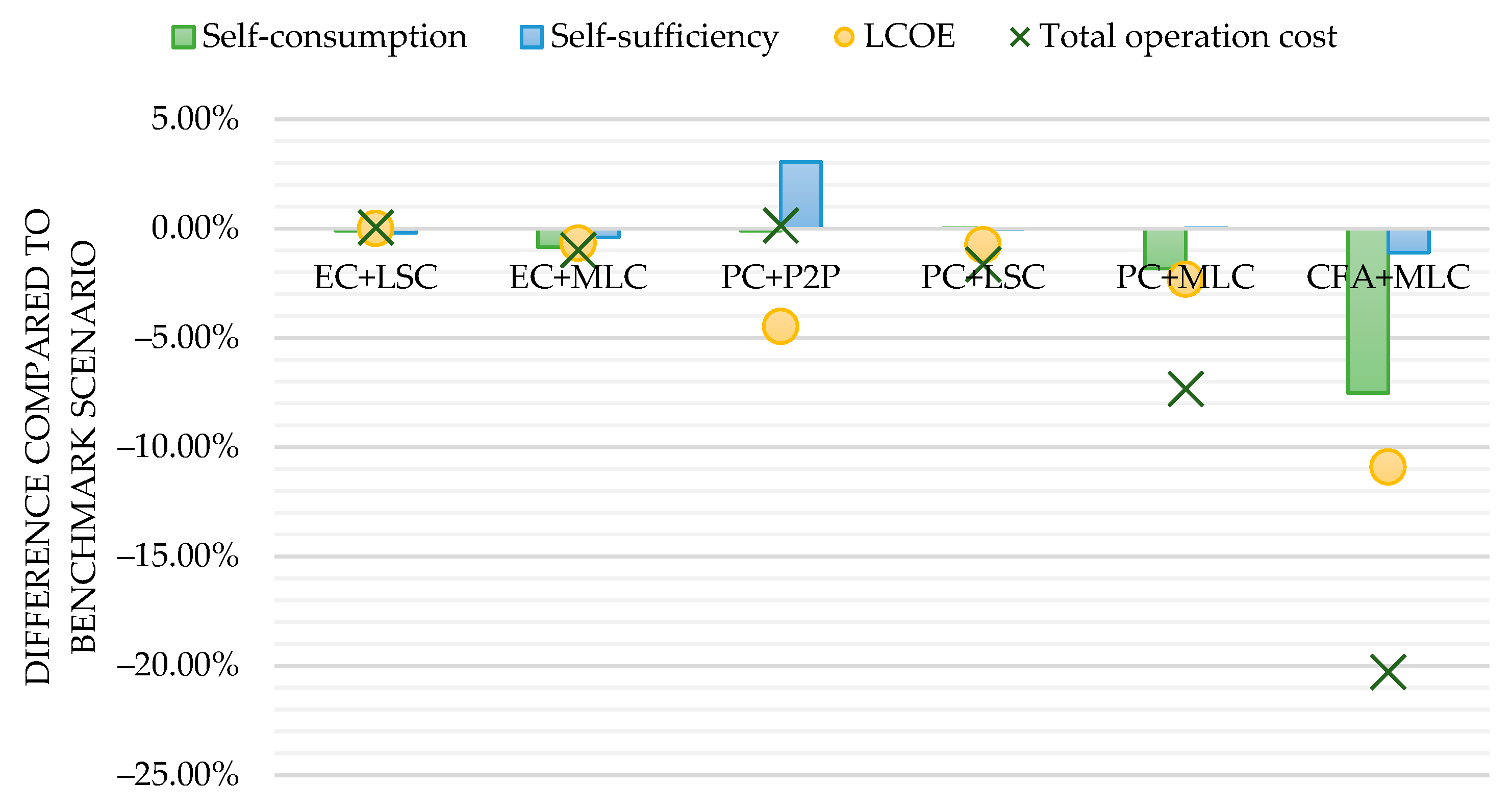
For this study, six scenarios and a benchmark case were simulated to investigate a LEC’s potential performance. The same LEC setup was used in each simulation, but the different business models and methods for asset dispatch in Table 1 were applied. To evaluate the performance of different scenarios, the simulation results are analysed using the indicators in Section 3 and Section 4. The relative difference in the performance of simulated scenarios compared to the benchmark scenario is provided in Figure 5.

The results of the benchmark scenario indicate that rule-based control of prosumer P_x provides considerably good results, as it provided the second highest self-consumption and third highest self-sufficiency rate compared to other scenarios while providing satisfactory economic performance. It can be concluded that if the sole aim of the LEC is to provide high levels of self-consumption, satisfactory results can be obtained using simple, rule-based control systems. Many state-of-the-art BESSs already provide an energy management system (EMS) to execute similar control as described in Figure A1, resulting in an inexpensive solution with relatively low computational requirements.

For the EC business model, insignificant differences exist between the simulation results of the maximisation of local self-consumption and the minimisation of LCOE. This is mainly due to the limited options for the LEC to influence its behaviour. Increased self-consumption also lowers the LCOE, which results in minimal differences between utilised asset dispatch methods.

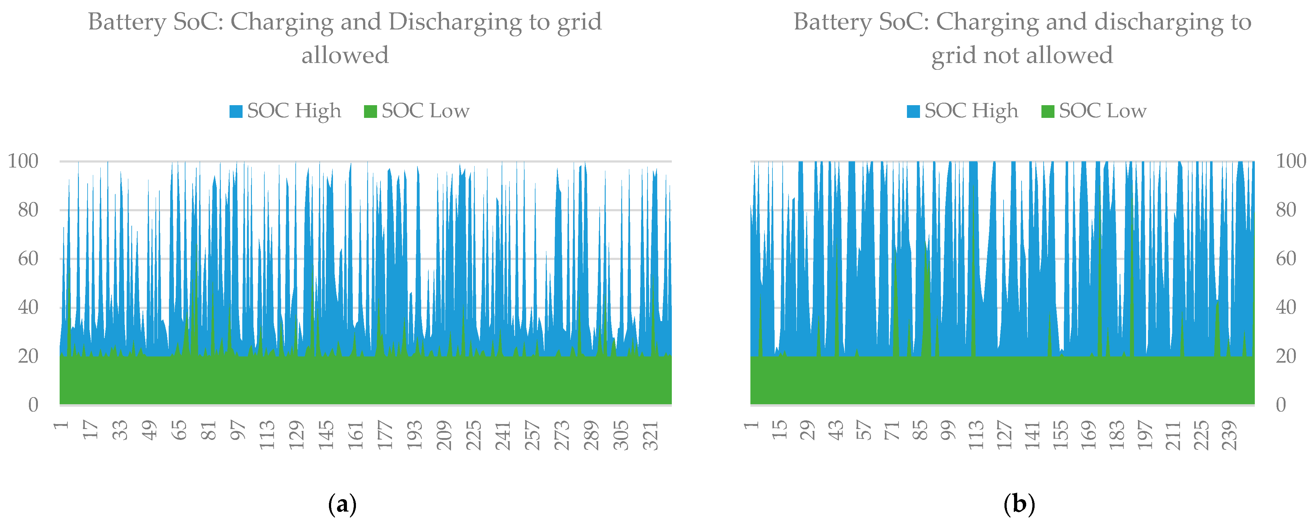
An interesting observation is that the results of the EC+LSC scenario provided a lower self-consumption value than what was obtained for the benchmark scenario. This is caused by constraints Equations (22) and (23), which prohibit the BESS from charging and discharging to the grid. When simulating the EC+LSC scenario without these constraints, the resulting self-consumption reaches a value of 93.13 %, which would result in the highest self-consumption rate, but the number of BESS charge and discharge cycles would also increase significantly. We analysed the BESS charge and discharge operations for both cases (the charging and discharging to the grid allowed and prohibited) of the EC+LSC scenario. A summary of general properties describing the studied cases is provided in

Table 4. Analysis of BESS charging and discharging cycles during the EC+LSC scenario for the cases of charging and discharging to the grid prohibited and allowed.

Case Description	Charging and Discharging to Grid Allowed	Charging and Discharging to Grid Are Not Allowed
Nr of cycles	332	252
Charge Median [% of BESS capacity]	21.59	53.84
Charge Average [% of BESS capacity]	35.33	49.43
Discharge Median [% of BESS capacity]	17.86	52.38
Discharge Average [% of BESS capacity]	33.91	49.43

, while the BESS utilisation analysis is provided in Appendix B. When charging and discharging to the grid is prohibited, the number of cycles is reduced, while charge and discharge cycles are deeper. When charging and discharging to the grid is allowed, the number of cycles is increased by over 30%, and each cycle’s depth is significantly lower than for the alternative case. The number of battery cycles affects their life cycle. Hence prohibiting the charge and discharge to the grid remained the preferred case in this study. We acknowledge that by modelling the impact of battery depletion into the optimisation algorithm, it would also consider the number of cycles and their depth of discharge. The improvement of the optimisation algorithm to consider the mentioned effects is the subject of future work.

The simulation results for the PC business model have a higher variance than the EC. This indicates that for LECs operated as PCs, the significance of choosing the suitable asset dispatch method is higher than for LECs operated as ECs. One scenario that stands out is the PC+P2P, which produced the highest ratio of self-sufficiency and the best LCOE for the PC business model. The PC+P2P scenario provided a better LCOE than the PC+MLC scenario while having only 0.1% less self-consumption than the PC+LSC scenario. This can be explained by the nature of the simulation, where the optimisation algorithm aims to match energy production and consumption inside the LEC by utilising flexibility, which results in similar self-consumption rates and total operational cost as the benchmark scenario, but significantly higher self-sufficiency, which lowers the LCOE. Simulating the P2P asset dispatch with improved flexibility characterisation is a point of interest for future studies. Additionally, simulating and comparing operational P2P algorithms to the results obtained in this study are in the scope of future research.

When comparing the performance of the LSC asset dispatch method, the self-consumption values between the benchmark, EC+LSC and PC+LSC scenarios fall within 0.1%. The PC+LSC scenario produced the best values for LCOE and total operation cost, which can be accounted for by utilising flexibility. This indicates that different business models have an insignificant effect on maximising the self-consumption of the LEC.

The findings of the MLC asset dispatch method indicate, as predicted, that the use of power system flexibility has a considerable influence on the overall operating cost and the levelized cost of energy (LCOE). The lowest LCOE was achieved for the CFA+MLC scenario, where the LEC takes the role of the aggregator and provides grid services directly to the system operator. Since this work aimed to quantify the potential of different LEC business models and asset dispatch method combinations, the implementation and increased operation costs for the LEC to operate as an aggregator were neglected. The calculation of flexibility remuneration considering actual activations and providing detailed financial calculations for integrating and operating a virtual power plant by the LEC is the subject of future work.

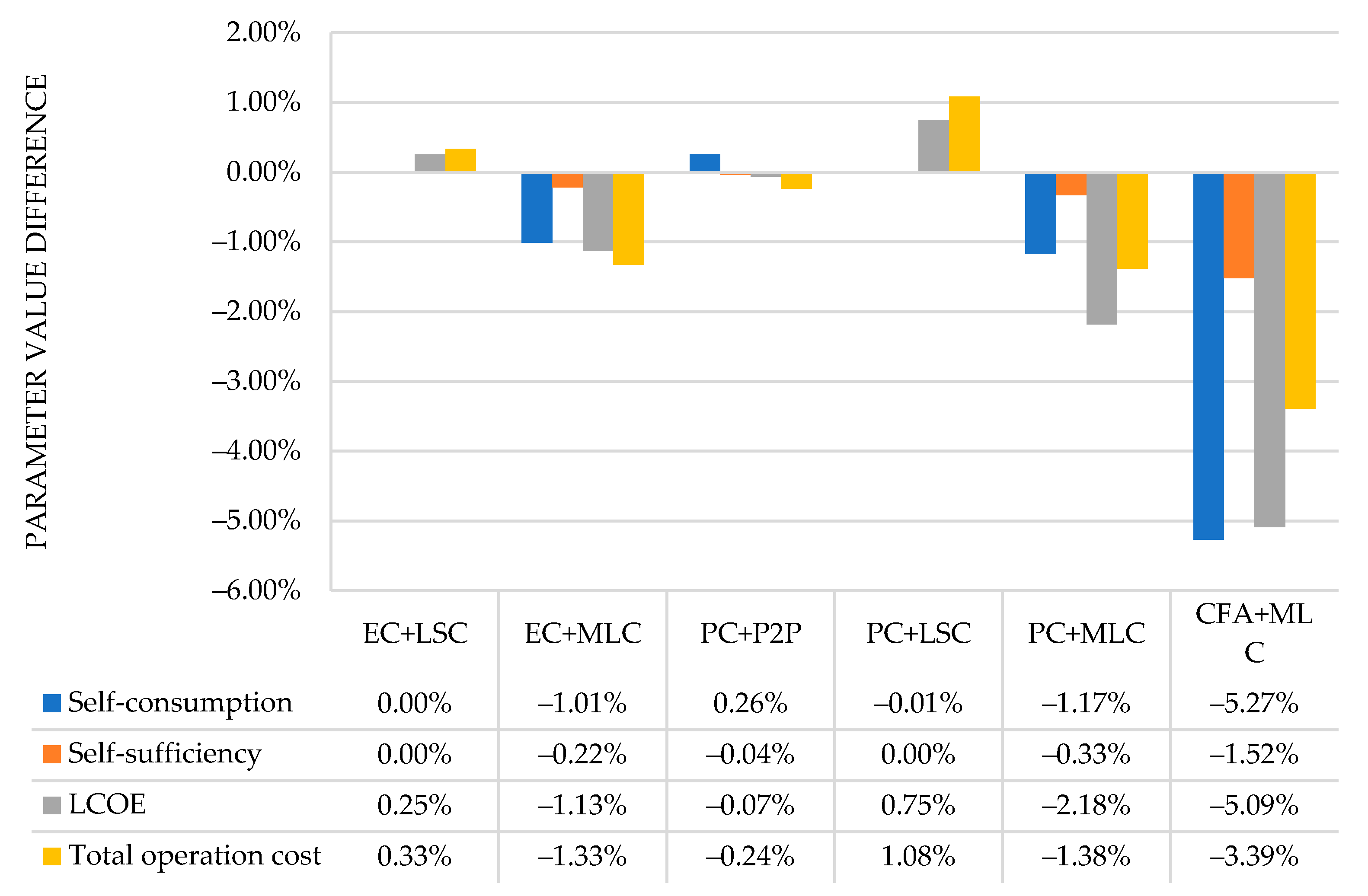
The same simulations were run using 2022 Nord Pool Spot Market pricing to further investigate how the Spot Market affected the simulation findings. The respective benchmark and results of the simulations with 2022 Spot Prices are summarised in

Table 5. Summary of simulation results with 2022 Nord Pool Spot Prices.

Parameter	Benchmark	EC+LSC	EC+MLC	PC+P2P	PC+LSC	PC+MLC	CFA+MLC
Self-consumption [%]	92.86	92.77	91.01	93.03	92.86	89.86	80.08
Self-sufficiency [%]	25.20	25.01	24.57	28.21	25.18	24.90	22.58
LCOE [€/kWh]	0.2000	0.2005	0.1964	0.1909	0.2000	0.1910	0.1680
Import cost [€]	90,421	90,908	89,595	90,384	90,492	85,052	84,869
Export revenue [€]	1889	2 040	3112	1942	1991	3644	13,171
Flexibility revenue [€]	-	-	-	-	466	591	4136
Total operation cost [€]	88,532	88,868	86,483	88,442	88,035	80,817	67,562

. The average energy prices on the Nord Pool Spot market in the EE price region were 0.087 €/kWh in 2021 and 0.192 €/kWh in 2022, corresponding to a price increase of 120.7%. Comparing benchmark values, self-consumption and self-sufficiency remain the same, while the LCOE increases by 49.5% and the total operation cost by 74.4%. Figure 6 displays the difference between the results of simulations that used 2021 and 2022 Nord Pool Spot market prices. The values displayed in Figure 6 are relative value differences, compared to respective benchmark values, between the results of simulations with different Nord Pool Spot market prices. As expected, the main differences are between LCOE and total operation cost, while the decrease is most notable for LECs utilising the MLC method for asset dispatch. For those LECs that utilise the MLC method for asset dispatch, it can be observed that the ratio of self-consumption is also decreasing. This means that under relatively high market prices, the LECs utilising the MLC asset dispatch method need to account for significantly reduced self-consumption.

Overall, it can be noted that the best PC+MLC and CFA+MLC scenarios give the best results from an economic point of view. However, the self-consumption and self-sufficiency are reduced in most cases. The PC+P2P and PC+LSC scenarios show lower improvements from the economic point of view, however, self-sufficiency and self-consumption never show significantly lower results compared to the benchmark case. Thus, the preferred combination depends on the overall goal for the LEC.

6. Conclusions

This study investigated the impact that different LEC business models and asset dispatch methods have on the performance potential of LECs. A benchmark and six scenarios were developed, modelled, and simulated using MILP. For each scenario, six key parameters were calculated and evaluated in order to estimate the prospective performance of the LECs and to benchmark their performance against other LECs. The key conclusions are stated below.

• If the LEC aims to provide high levels of self-consumption, while there exists a limited number of controllable assets, simple, rule-based control systems provide a solution with low computational complexity that is easy to implement.
• The utilisation of flexibility increases the LEC’s economic performance, but different asset dispatch methods provide different rates of self-sufficiency.
• When the LEC is utilising an energy cooperative business model, the selected asset dispatch method provides only minor differences in LEC performance.
• For LECs operated as prosumer communities, the significance of choosing the suitable asset dispatch method is higher than those operating as energy cooperatives.
• The LEC’s business model has an insignificant effect on maximising its self-consumption.
• For LECs operated as prosumer communities, the P2P asset dispatch method can provide a lower LCOE than other asset dispatch methods while realising that potential through operational P2P algorithms remains to be verified.
• The LEC has the potential to significantly increase its economic performance by taking the role of the aggregator and directly providing grid services to system operators.
• Increased energy prices reduce the self-consumption of the LECs that utilise the MLC asset dispatch method.

As a result of this work, we have quantified the potential of different LECs, the outcomes of this work will serve as a benchmark for evaluating the effectiveness of various operational optimisation and control techniques, which is the subject of future work. Secondly, the aim is to improve the presentation of prosumer flexibility availability and delivery, where data about power system flexibility requirements, activations and respective remuneration is included. The calculation of flexibility remuneration considering actual activations and providing detailed financial calculations for integrating and operating a virtual power plant by the LEC is the subject of future work, as well as simulating the P2P asset dispatch with improved flexibility characterisation. Another focus lies in improving the optimisation algorithm to consider the degradation of the battery based on BESS usage.

References

1. Korõtko, T.; Drovtar, I.; Mutule, A.; Kairisa, E.; Rosin, A. Load Flow Modelling in Local Energy Community Electric Power Systems. In Proceedings of the 2022 IEEE 7th International Energy Conference (ENERGYCON), Riga, Latvia, 9–12 May 2022; pp. 1–7. [Google Scholar] [CrossRef]
2. Ahmadiahangar, R.; Baharvandi, A.; Rosin, A.; Häring, T.; Azizi, E.; Korõtko, T.; Shabbir, N. Energy Storage Expansion Planning In Microgrid. In Proceedings of the 2020 IEEE 14th International Conference on Compatibility, Power Electronics and Power Engineering (CPE-POWERENG), Setubal, Portugal, 8–10 July 2020; pp. 433–437. [Google Scholar] [CrossRef]
3. Häring, T.; Kull, T.M.; Ahmadiahangar, R.; Rosin, A.; Thalfeldt, M.; Biechl, H. Microgrid Oriented modeling of space heating system based on neural networks. J. Build. Eng. 2021, 43, 103150. [Google Scholar] [CrossRef]
4. Ahmadiahangar, R.; Azizi, E.; Sahoo, S.; Häring, T.; Rosin, A.; Vinnikov, D.; Dragicevic, T.; Beheshti, M.T.H.; Blaabjerg, F. Flexibility investigation of price-responsive batteries in the microgrids cluster. In Proceedings of the 2020 IEEE 14th International Conference on Compatibility, Power Electronics and Power Engineering (CPE-POWERENG), Setubal, Portugal, 8–10 July 2020; pp. 456–461. [Google Scholar] [CrossRef]
5. Maask, V.; Häring, T.; Ahmadiahangar, R.; Rosin, A.; Korõtko, T. Analysis of Ventilation Load Flexibility Depending on Indoor Climate Conditions. In Proceedings of the 2020 IEEE International Conference on Industrial Technology (ICIT), Buenos Aires, Argentina, 26–28 February 2020; pp. 607–612. [Google Scholar] [CrossRef]
6. Drovtar, I.; Korõtko, T.; Mutule, A.; Kairisa, E.; Rosin, A. Determining optimisation Framework for Local Energy Communities. In Proceedings of the 2022 IEEE 7th International Energy Conference (ENERGYCON), Riga, Latvia, 9–12 May 2022; pp. 1–7. [Google Scholar] [CrossRef]
7. Bahlke, F.; Liu, Y.; Pesavento, M. Stochastic load scheduling for risk-limiting economic dispatch in smart microgrids. In Proceedings of the 2016 IEEE International Conference on Acoustics Speech and Signal Processing (ICASSP), Shanghai, China, 20–25 March 2016; pp. 2479–2483. [Google Scholar] [CrossRef]
8. de la Nieta, A.A.S.; Gibescu, M.; Wang, X.; Song, M.; Jensen, E.; Saleem, A.; Bremdal, B.; Ilieva, I. Local Economic Dispatch with Local Renewable Generation and Flexible Load Management. In Proceedings of the 2018 International Conference on Smart Energy Systems and Technologies (SEST), 10–12 September 2018; pp. 1–6. [Google Scholar] [CrossRef]
9. Sasaki, Y.; Ueoka, M.; Yorino, N.; Zoka, Y.; Bedawy, A.; Kihembo, M.S. Dynamic Economic Load Dispatch with Emergency Demand Response for Microgrid System Operation. In Proceedings of the 2021 22nd International Middle East Power Systems Conference (MEPCON), Assiut, Egypt, 14–16 December 2021; pp. 497–502. [Google Scholar] [CrossRef]
10. Jordehi, A.R.; Javadi, M.S.; Catalão, J.P.S. Dynamic Economic Load Dispatch in Isolated Microgrids with Particle Swarm Optimisation considering Demand Response. In Proceedings of the 2020 55th International Universities Power Engineering Conference (UPEC), Turin, Italy, 1–4 September 2020; pp. 1–5. [Google Scholar] [CrossRef]
11. Lazdins, R.; Mutule, A.; Zalostiba, D. PV Energy Communities—Challenges and Barriers from a Consumer Perspective: A Literature Review. Energies 2021, 14, 4873. [Google Scholar] [CrossRef]
12. Reis, I.F.; Gonçalves, I.; Lopes, M.A.; Antunes, C.H. Business models for energy communities: A review of key issues and trends. Renew. Sustain. Energy Rev. 2021, 144, 111013. [Google Scholar] [CrossRef]
13. Girish, P.; Yuvaraj, T.; Hariharan, R. Solution for economic load dispatch problem using optimisation algorithm—Review. Int. J. Pure Appl. Math. 2018, 119, 263–269. [Google Scholar]
14. Nouri, A.; Khadem, S.; Mutule, A.; Papadimitriou, C.; Stanev, R.; Cabiati, M.; Keane, A.; Carroll, P. Identification of gaps and barriers in regulations, standards, and network codes to energy citizen participation in the energy transition. Energies 2022, 15, 856. [Google Scholar] [CrossRef]
15. Caramizaru, E.; Uihlein, A. Energy Communities: An Overview of Energy and Social Innovation; EUR 30083 EN; Publications Office of the European Union: Luxembourg, 2020. [Google Scholar] [CrossRef]
16. REScoop. Available online: https://www.rescoop.eu/ (accessed on 2 December 2022).
17. Bauwens, T.; Gotchev, B.; Holstenkamp, L. What drives the development of community energy in Europe? The case of wind power cooperatives. Energy Res. Soc. Sci. 2016, 13, 136–147. [Google Scholar] [CrossRef]
18. Wierling, A.; Schwanitz, V.J.; Zeiß, J.P.; Bout, C.; Candelise, C.; Gilcrease, W.; Gregg, J.S. Statistical Evidence on the Role of Energy Cooperatives for the Energy Transition in European Countries. Sustainability 2018, 10, 3339. [Google Scholar] [CrossRef]
19. Brown, D.; Hall, S.; Davis, M.E. Prosumers in the post subsidy era: An exploration of new prosumer business models in the UK. Energy Policy 2019, 135, 110984. [Google Scholar] [CrossRef]
20. Eurelectric, Citizens Energy Communities: Recommendations for a Successful Contribution to Decarbonisation—A Eurelectric Position Paper, Eurelectric. 2019. Available online: https://www.apren.pt/contents/publicationsothers/eurelectric--citizens-energy-communities.pdf (accessed on 14 April 2023).
21. Reins, L. Residential Prosumers in the European Energy Union—Mapping the Legal and Regulatory Framework in Germany. Milieu Ltd. 2017. Available online: https://ec.europa.eu/commission/publications/accompanying-documents-state-energy-union_en (accessed on 2 December 2022).
22. Brown, D.; Hall, S.; Davis, M.E. What is prosumerism for? Exploring the normative dimensions of decentralised energy transitions. Energy Res. Soc. Sci. 2020, 66, 101475. [Google Scholar] [CrossRef]
23. Korõtko, T.; Rosin, A.; Ahmadiahangar, R. Development of Prosumer Logical Structure and Object Modeling. In Proceedings of the 2019 IEEE 13th International Conference on Compatibility, Power Electronics and Power Engineering (CPE-POWERENG), Sonderborg, Denmark, 23–25 April 2019; pp. 1–6. [Google Scholar] [CrossRef]
24. Plaum, F.; Ahmadiahangar, R.; Rosin, A.; Kilter, J. Aggregated demand-side energy flexibility: A comprehensive review on characterisation, forecasting and market prospects. Energy Rep. 2022, 8, 9344–9362. [Google Scholar] [CrossRef]
25. Plaum, F.; Ahmadiahangar, R.; Rosin, A. Aggregated Energy Flexibility Provision Using Residential Heat Pumps. In Proceedings of the 2022 IEEE 16th International Conference on Compatibility, Power Electronics, and Power Engineering, CPE-POWERENG 2022, Birmingham, UK, 29 June–1 July 2022. [Google Scholar] [CrossRef]
26. Zolfaghari, M.; Ahmadiahangar, R.; Gharehpetian, G.B.; Rosin, A.; Plaum, F. Using V2G Technology as Virtual Active Power Filter for Flexibility Enhancement of HVDC Systems. In Proceedings of the 2020 IEEE 14th International Conference on Compatibility, Power Electronics and Power Engineering, CPE-POWERENG, Setubal, Portugal, 8–10 July 2020; pp. 489–494. [Google Scholar] [CrossRef]
27. Good, N.; Ellis, K.A.; Mancarella, P. Review and classification of barriers and enablers of demand response in the smart grid. Renew. Sustain. Energy Rev. 2017, 72, 57–72. [Google Scholar] [CrossRef]
28. Neska, E.; Kowalska-Pyzalska, A. Conceptual design of energy market topologies for communities and their practical applications in EU: A comparison of three case studies. Renew. Sustain. Energy Rev. 2022, 169, 112921. [Google Scholar] [CrossRef]
29. Casals, X.; Sanmartí, M.; Salom, J. Smart Energy Communities: Insights into Its Structure and Latent Business Models; Institut Català d’Energia-Institut de Recerca en Energia de Catalunya (IREC): Barcelona, Spain, 2019. [Google Scholar]
30. Rajabi, A.; Li, L.; Zhang, J.; Zhu, J. Aggregation of small loads for demand response programs—Implementation and challenges: A review. In Proceedings of the 2017 IEEE International Conference on Environment and Electrical Engineering and 2017 IEEE Industrial and Commercial Power Systems Europe (EEEIC/I&CPS Europe), Milan, Italy, 6–9 June 2017; IEEE: Piscataway, NJ, USA, 2017; pp. 1–6. [Google Scholar]
31. Maksimovich, V. Analysis of Capabilities of Machine Learning for Local Energy Communities to Provide Flexibility to the Grid; Escola Tècnica Superior d’Enginyeria Industrial de Barcelona (UPC): Barcelona, Spain, 2021. [Google Scholar]
32. The OpenADR Primer: An introduction to Automated Demand Response and the OpenADR Standard. Available online: https://www.openadr.org/assets/docs/openadr_primer.pdf (accessed on 18 December 2022).
33. Huld, T.; Müller, R.; Gambardella, A. A new solar radiation database for estimating PV performance in Europe and Africa. Solar Energy 2012, 86, 1803–1815. [Google Scholar] [CrossRef]
34. Nord Pool Day-Ahead Prices. Available online: https://www.nordpoolgroup.com/en/Market-data1/Dayahead/Area-Prices/EE/Yearly/?view=table (accessed on 3 February 2023).
Figure 1. LEC organised as Energy Cooperative.
Energies 16 03476 g001
Figure 2. LEC organised as Community of Prosumers.
Energies 16 03476 g002
Figure 3. LEC organised as Community for Flexibility Aggregation.
Energies 16 03476 g003
Figure 4. Topology of the LEC power system used in the case study.
Energies 16 03476 g004
Figure 5. The relative difference in the performance of simulated scenarios compared to the benchmark scenario; self-consumption, self-sufficiency: higher is better; LCOE, total operation cost: lower is better.
Energies 16 03476 g005
Figure 6. Differences between scenario simulation results (compared to benchmark) with different Nord Pool Spot market data. Simulation results with 2021 and 2022 Nord Pool Spot market prices are compared. Self-consumption, self-sufficiency: negative values show better performance with 2021 Nord Pool Spot market prices than with 2022 prices and vice versa; LCOE, Total operation cost: positive values show better performance with 2021 Nord Pool Spot market prices than with 2022 prices and vice versa.
Energies 16 03476 g006