
On the Summarization of Meteorological Data for Solar Thermal Power Generation Forecast

1
Industrial Engineering Program (PEI), Federal University of Bahia (UFBA), Salvador 40210-630, BA, Brazil
2
Excellence Group in Thermal Power and Distributed Generation (NEST), Federal University of Itajubá (UNIFEI), Itajubá 37500-005, MG, Brazil
*
Author to whom correspondence should be addressed.
Energies 2023, 16(7), 3297; https://doi.org/10.3390/en16073297
Submission received: 15 February 2023
/
Revised: 24 March 2023
/
Accepted: 4 April 2023
/
Published: 6 April 2023
(This article belongs to the Section A2: Solar Energy and Photovoltaic Systems)
Abstract
:The establishment of the typical weather conditions of a given locality is of fundamental importance to determine the optimal configurations for solar thermal power plants and to calculate feasibility indicators in the power plant design phase. Therefore, this work proposes a summarization method to statistically represent historical weather data using typical meteorological days (TMDs) based on the cumulative distribution function (CDF) and hourly normalized root mean square difference (nRMSD). The proposed approach is compared with regular Sandia selection in forecasting the electricity produced by a solar thermal power plant in ten different Brazilian cities. Considering the determination of the annual generation of electricity, the results obtained show that when considering an overall average of weather characteristics, commonly used for analyzing solar thermal power plant designs, the normalized mean average error (nMAE) is 20.8 ± 4.8% relative to the use of historical data of 20 years established at hourly intervals. On the other hand, a typical meteorological year (TMY) is the most accurate approach (nMAE = 1.0 ± 1.1%), but the costliest in computational time (CT = 381.6 ± 56.3 s). Some TMD cases, in turn, present a reasonable trade-off between computational time and accuracy. The case using 4 TMD, for example, increased the error by about 11 percentual points while the computational time was reduced by about 81 times, which is quite significant for the simulation and optimization of complex heliothermic systems.
1. Introduction
The best use of energy sources, especially renewable ones, is the most concrete way to lead electricity production to the net zero carbon emissions goal [1,2]. Solar photovoltaic and wind are running in this direction, but at a rate lower than expected in the IEA net zero scenario [3]. Solar thermal (heliothermic) electricity generation is at an even slower pace, and although there are facilities already operating worldwide, an increase in the production of their components is necessary for these systems to reach maturity, reliability, and economic viability.
Weather forecast plays an important role in the indication of the optimal configuration of thermal systems, especially on the heliothermic case. The efficiency of solar collectors is dependent on the direct normal irradiance (DNI), local dry bulb temperature, and wind velocity, which determines the convection losses. The power block efficiency is a function of the local dry or wet bulb temperature, according to the selected condensation system. The energy loss from storage tanks depends on the dry bulb temperature and wind velocity. Nevertheless, the heat loss from the collectors absorber is a percentage of heat absorbed at the given moment, which in turn is a function of momentary DNI, solar incidence angle, and wind velocity. Thus, for the correct prediction of the electricity generated by these systems, it is necessary to have a representative distribution of each meteorological characteristic and a proper match between them at every moment. This is particularly critical for optimization codes in which it is necessary to assess the power produced by the configuration under selection in each loop of the optimization process.
It is common to represent weather conditions as a typical meteorological year (TMY) statistically representative of all the variables that influence the energy production of the studied power plant [4], building energy simulation [5], and even climate change studies [6]. The selection of TMY depends on the approach used. Hall et al. [7] used the Finkelstein–Schafer statistic and a persistence criterion (Sandia method). Andersen et al. [8] relied on Fourier analysis and qualification based on standard deviation (Danish method). Crow [9] proposed the use of Sandia or Danish selection with post-processing replacing hourly or daily weather values to lead the monthly mean value closer to the respective long-term value (Crow method). Gazela and Mathioulakis [10] applied a system-oriented model based on minimization of the error in the monthly prediction, which is compared with the mean solar gain of the long-term data set. The Finkelstein–Schafer statistic is used to compare a candidate and the historic data set in most applications. This approach was applied for different locations, such as Greece [11], China [12], Togo [13], Argentina [14], and Brazil [15], and it usually chooses representatives that are close to historical data [16].
Some works addressing the issue of weather representation to be used in forecasting electricity generation can be found in the literature. Most methods employed are based on statistical, physical, machine learning, and hybrid approaches [17,18]. Law et al. [19] compared the effect of the accuracy of three forecast methods on the financial value of a concentrated solar thermal (CST) plant. Results of persistence; autoregressive integrated moving average (ARIMA); and air pollution model (TAPM) were compared with the measured values from Mildura, Australia, for the period of 1 June to 30 November 2005. Based on mean bias error (MBE), mean absolute error (MAE), and root mean square error (RMSE), the authors concluded that, although the persistence model was more consistent, i.e., MAE close to zero, its errors are larger than those of ARIMA and TAPM. Luo and Zhang [20] proposed an adaptative deep learn long short-term memory (AD-LSTM) model to forecast photovoltaic systems power generation. This model uses historical data to predict future weather conditions, but it dynamically learns with recent reading data. The AD-LSTM improves forecast skills by up to 73.11% for day-ahead power generation forecasts showing superior performance when compared to other proposed models, such as offline LSTM (OL-LSTM). Rana et al. [21] presented different convolutional neural network (CNN) models for forecasting the power generated by solar thermal power systems over multiple time horizons simultaneously. These models were compared with historical data from evacuated collectors and linear Fresnel collectors. Experimental results reveal a mean percentage error (MAPE) between 2.99% and 4.18% for a 30 min time step dataset and 24 h-ahead prediction, respectively.
Steady-state and dynamic modeling of solar systems are computationally expensive, and the greater the time discretization degree, the longer the analysis duration. This increase in processing time is more relevant when optimizations are applied since the meteorological data must be considered at every loop of the optimization process. So, it is common to use fixed irradiance during optimizations [22] which can lead to under or over-dimensioned systems since the components efficiency is sensitive to fluctuations of environmental conditions.
Vasallo and Bravo [23] evaluated a 50 MW power plant based on concentrated solar power (CSP) using parabolic trough collectors and thermal storage aiming to optimize power scheduling. The weather conditions considered were based on a single day (21 March 2013, Granada, Spain), and their dynamic model used linear interpolation to determine weather conditions. Monjurul Ehsan et al. [24] performed the optimization of a central tower solar thermal power plant with energy storage and a dry-cooled supercritical CO2 power block. The optimization was performed at a fixed design condition of DNI and two design points for air temperature. The authors concluded that the correct selection of design conditions is crucial, recommending the use of a design condition between the mean value and the highest frequency value for meteorologic inputs. This approach may result in considerable discrepancies in relation to the annual operation of the plant. Brodrick et al. [25] performed the optimization of a coal-gas-solar hybrid system with carbon capture. The solar data were obtained from the National Solar Radiation Database (NSRDB) [26] with a time step of 2 h for the year 2010. Their algorithm was capable of consistently maximizing the net present value (NPV) using up to eight statistically representative days. Orsini et al. [27] optimized a parabolic trough plant with energy storage using particle swarm optimization—mesh adaptive direct search (PSO-MADS). Similar to Brodrick et al. [25], these authors represented local weather conditions of the year 2017 with four representative days, each representing a season.
Despite the vast availability of works related to the prediction of solar irradiation based on typical meteorological years, few papers approach periods shorter than one year. The novelty of this work lies on the development, comparison, and discussion of different approaches for the summarization of historic meteorological data set in typical meteorological day(s) (TMD) using a modified Sandia method. This approach is used to enable complex optimizations that otherwise would be inviable due to required computational time. Ten different Brazilian locations were used as a case study and the results were compared with data from the historical period.
2. Methodology
This section describes the Sandia method used to obtain a typical meteorological year (TMY) and the proposed adaptations for condensation of historic meteorological data set in shorter periods of time.
2.1. Sandia Selection and Proposed Adoptations
The Sandia selection is a statistical method developed to select a TMY, which is used to replace long-term meteorological data, such as 30 years, so that technical and economical evaluations can be performed with reduced computational burden. This typical year is a composition of representative months selected from the long-term meteorological data set. The Sandia method was originally developed by the National Renewable Energy Laboratory (NREL) [28] and revised by Marion and Urban [29] until reaching its last version proposed by Wilcox and Marion [30].
The selection criteria used for the construction of a TMY in this work is an adaptation of the original method, and it is based on the following steps:
- The cumulative distribution function (CDF) of the meteorological characteristic under evaluation, e.g., temperature, of each candidate (month) is compared to the CDF of the respective months of the long-term meteorological data set. The Finkelstein–Schafer (FS) statistic [31] definition, Equation (1), is used to perform the CDF comparison.
In Equation (1), represents the absolute difference between the CDF of the candidate and the respective months from a long-term meteorological data set, while is the number of readings of the jth meteorological characteristic and is the reading value [30].
The final FS statistic is computed as a weighted average considering each statistic, as shown in Equation (2).
In Equation (2), is the weight of each jth meteorological characteristic.
- 2.
- The candidates are ranked according to its FS-statistic, the lower the better, and the top five candidates are selected to the next step;
- 3.
- The top five candidates are evaluated in terms of frequency and length of “runs”, i.e., values for the meteorological characteristic under evaluation over (67th percentile) or below (33rd percentile) the expected range of values. This persistence test excludes the candidate (month) with the longest run (more consecutive days with meteorological characteristic out of expected values), the candidate with the most runs, and a possible candidate with zero runs;
- 4.
- For the remaining candidates, the hourly meteorological characteristic is compared to the hourly average value of the equivalent month from the long-term data set () using the weighted normalized root mean square difference (nRMSD), Equation (3). This slight adaptation of the Sandia method is used to improve the hourly matching of different meteorological characteristics. Pissimanis et al. [32] proposed this step as a replacement for the persistence test (Step 3); here, it is used to increase selection rigor. The normalization is applied by dividing each RMSD for the jth meteorological characteristic by the long-term average, Equation (4);
- 5.
- The twelve selected months are concatenated to compose the TMY.
This work considers the effective direct normal irradiance (eDNI), wind velocity, and ambient temperature (dry bulb) to select the representative months using the weights indicated in Table 1, since these are the most significant variables affecting collectors efficiency. The , Equation (5), condenses DNI and incidence angle in a single variable.
2.2. Adaptations to Obtain a Typical Meteorological Day
A typical meteorological day (TMD) can be obtained following the same steps indicated in Section 2.1. Two minor adaptations are necessary: (i) the frequency and length of runs are evaluated in terms of consecutive hours instead of days as in the original method; (ii) the hourly meteorological characteristic of each candidate (day) is compared to the hourly mean long-term meteorological characteristic in Step 4.
Some options for using TMD are: (i) one day to represent the entire period; (ii) 4 days to represent the entire period, one for each season; (iii) 12 days to represent the entire period one for each month of the period; and (iv) 73 days to represent the entire period, one for each 5-day week of the historical period.
2.3. Performance Metrics
The comparison between approaches, TMY and TMD options, is based on the absolute error (nAE) of the forecast for the electricity produced in 20 years using a solar thermal power plant. The electricity production forecast is compared to the forecast obtained using the entire historic data set from 2001 to 2020 () for each selected location, Equation (6). The normalized mean absolute error (nMAE) is then calculated based on the nAE for the N locations, Equation (7).
In Equation (6) is the 20-year electricity production forecast for each approach.
3. Case Studies
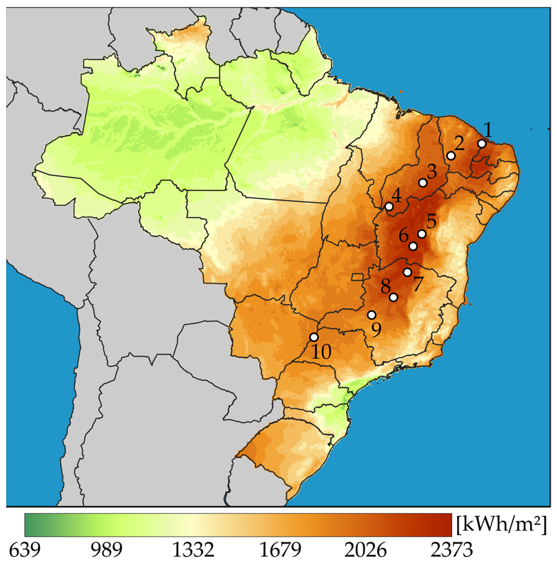
Ten Brazilian cities were selected in order to test the TMD options, see Figure 1 and Table 2. These locations were chosen to cover different latitudes of the Brazilian territory. The weather data were obtained from the National Solar Radiation Database (NSRDB) [26].
The effect of the proposed approaches in solar thermal power plants is evaluated using the electricity production forecast for the next 20 years. The plant used for this evaluation is composed of two storage tanks (ST), i.e., a direct storage system, an organic Rankine cycle power block (PB), and a solar field (SF) of parabolic trough collectors. Table 3 shows the characteristics of the plant main components. These parameters are fixed and were obtained by optimization aiming maximization of the internal rate of return for an annual generation of 17 MWh using 1 TMD at Bom Jesus da Lapa–BA (id. 6).
4. Results and Discussion
Figure 2 indicates the effect of Step 4 into the 1 TMD selection procedure for Bom Jesus da Lapa–BA (id. 6). Huge hourly deviations in relation the long-term average are reduced. Although only eDNI is presented, other properties are also being used for the selection and will be used to calculate the plant electricity generation forecast. Thus, a more representative matching of properties for each hour is expected while the cumulative distribution is not significantly affected since this criterion is applied to the top five candidates.
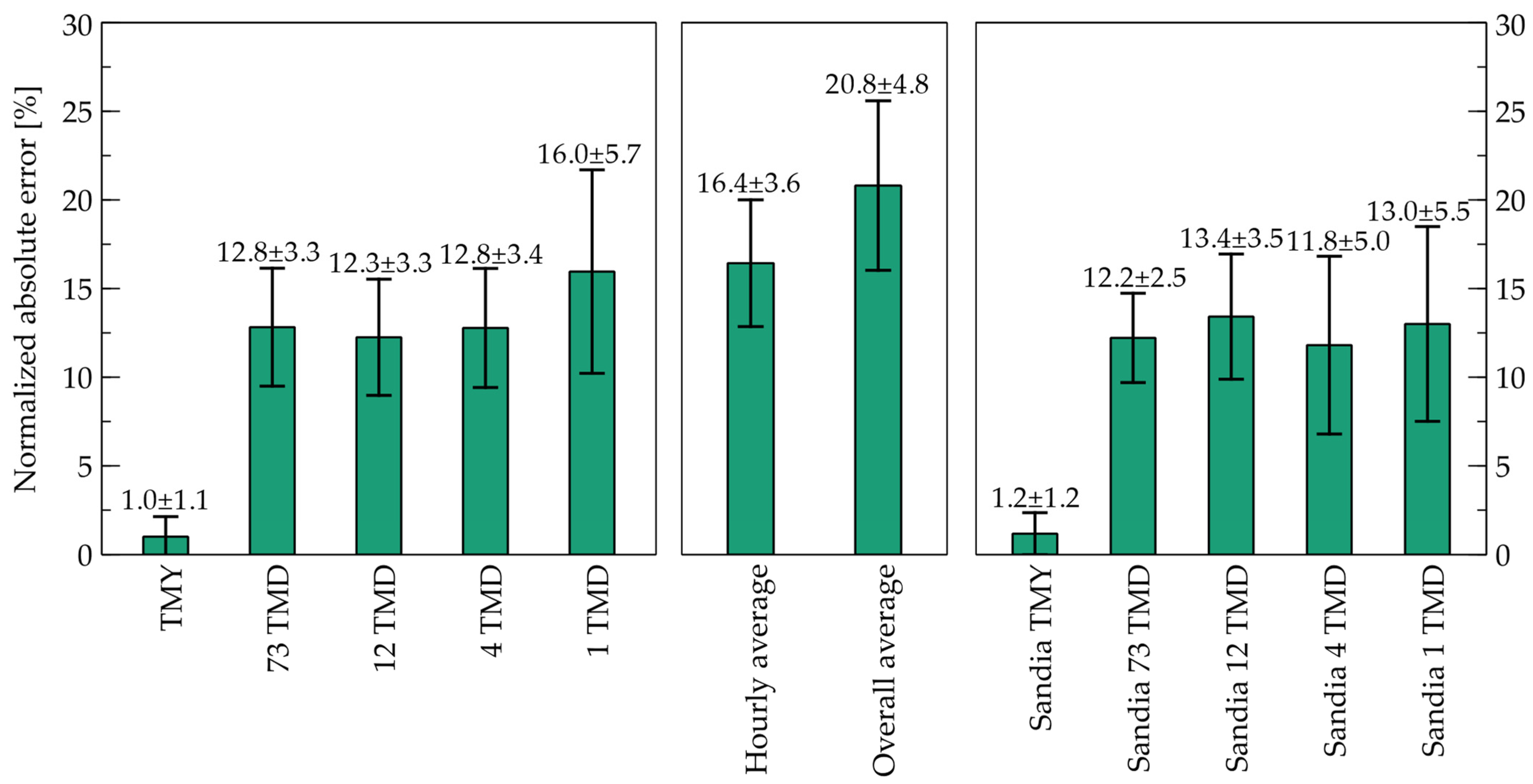
Figure 3 indicates the error for electricity production forecast. For the sake of comparison, two simple approaches were included: (i) the hourly average, i.e., one representative day created using the average of each hour, and (ii) the overall average, i.e., a single average representing the whole period. Figure 3 reveals that the TMYs obtained from both approaches (Sandia and proposed) produce results very close to those obtained using all the hours of the historic data set (20 years). It is interesting to note that use of 4, 12, and 73 TMDs produces about the same error. No significant improvement was noted when Step 4 was included. It is possible to infer that the benefit from a better matching of properties is too small in relation to the errors associated with the forecast. The hourly average produces an error slightly higher than 1 TMD and higher than Sandia 1 TMD. It is expected that the hourly average produces a larger error since the lower and higher values of weather characteristics under evaluation are important for electricity production forecast, i.e., they have a non-linear influence on collectors efficiency, heat loss, radiation absorption, etc. When the values are “averaged” the non-linear influence of the extremes is lost. This effect is more evident for the overall average, which produces an error of about 21%.
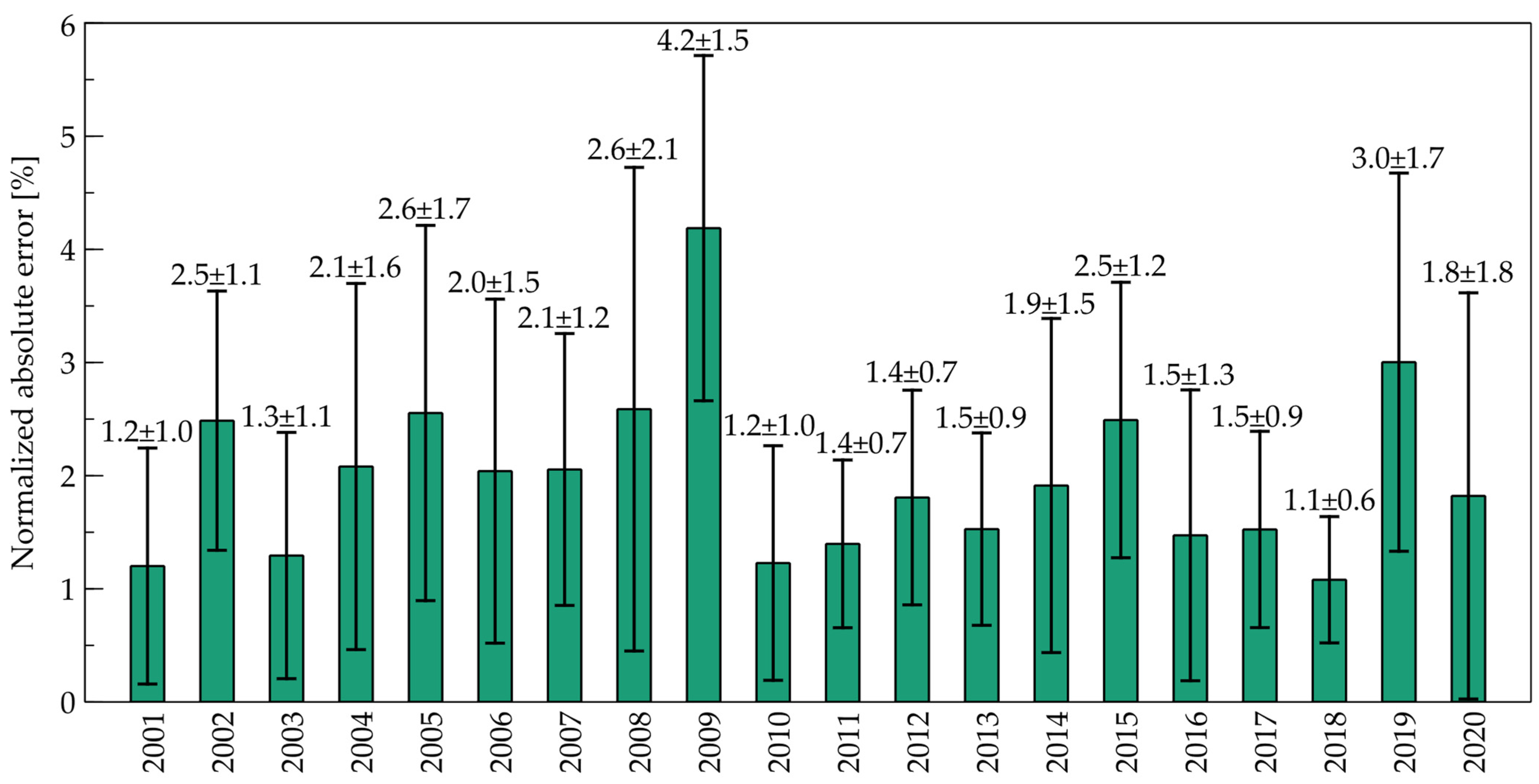
Figure 4 further indicates that the use of real year from historic period produces almost the same effect of TMY on electricity production. The years 2001, 2003, 2020, and 2018, TMY and TMY Sandia have errors within the same order of magnitude and can be considered good representatives for the entire period.
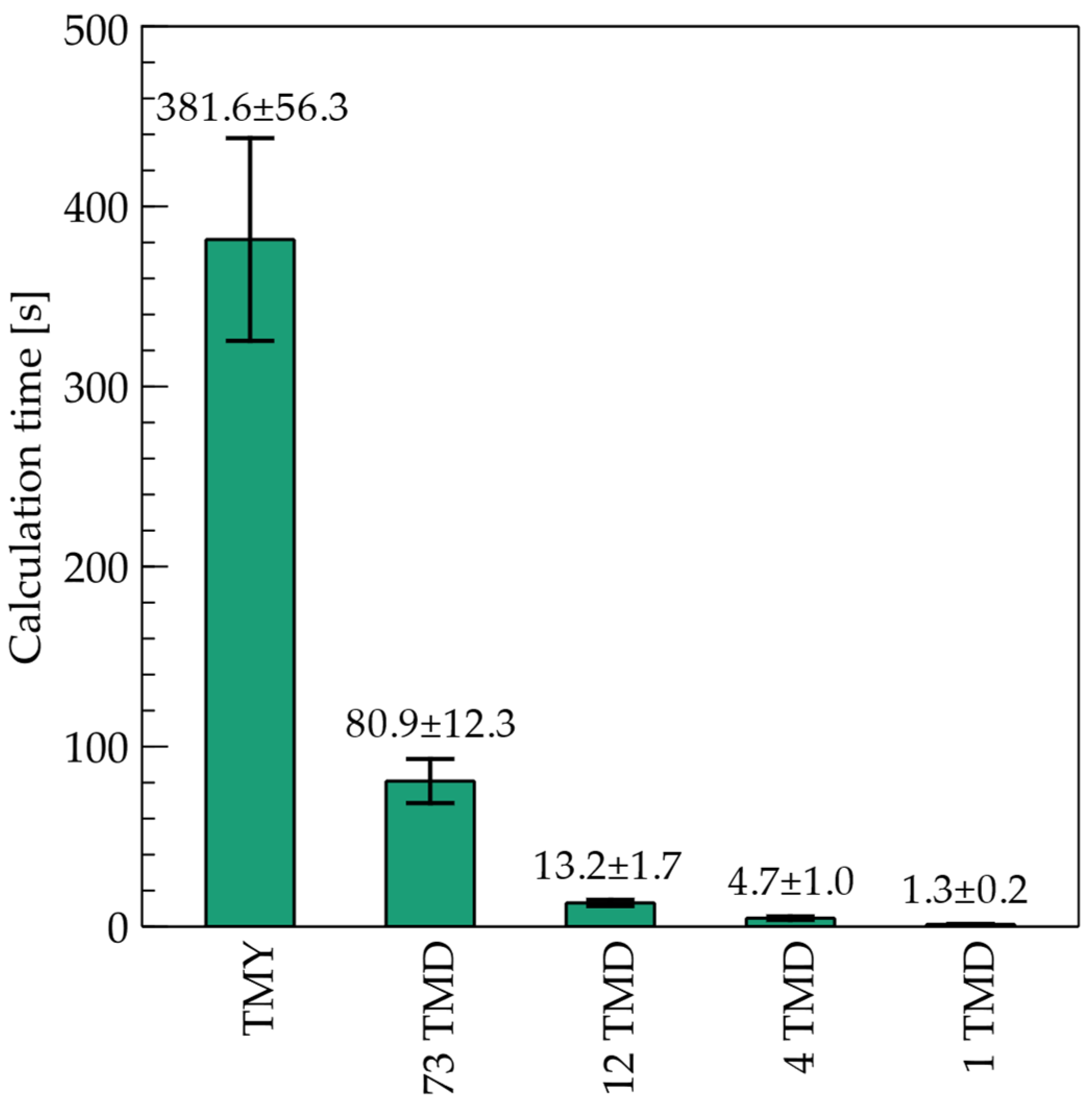
Figure 5 shows the computational time for the analyzed approaches. The computational time is proportional to the number of days used in the analysis; thus, by using 1 TMD instead of TMY or an actual historic year, a reduction of approximately 365 times is observed. By analyzing Figure 3 and Figure 5, it is possible to indicate that the use of 4 TMD and 4 TMD Sandia may imply a reasonable trade-off between accuracy and processing time, i.e., a reduction in accuracy of about 11 percentual points supported by a reduction in the processing time of about 81 times compared with TMY and TMY Sandia. This reduction is especially important in optimization routines in which the time saving between 4 TMDs and TMY can reach 1047 h (43.6 days) for a genetic algorithm with 100 generations and 100 individuals per generation. Nevertheless, the 4 TMD and 4 TMD Sandia could be used for plant optimization and the TMY can be used to forecast more accurately the electricity generated by the configuration selected during the optimization process; this combined approach is used in [33]. It is important to emphasize that there is an unavoidable error in using historical data to forecast future weather conditions. Therefore, very high precision, in respect to the past, may not improve the forecast and may add a large computational burden. Thus, computation burden and precision in respect to the past must be properly weighted and the best choice depends on the application aimed.
5. Conclusions
This work presented a method to summarize historical weather data into a statistical representative day, called a typical meteorological day (TMD). This day can represent any specific period of a year, thus more than one day can be used to represent a typical year. Ten Brazilian cities covering different latitudes in Brazilian sun belt were used to analyze the errors involved in the electricity production forecast from a solar thermal power plant using the proposed approaches.
An error of about 20.8 ± 4.8% was observed by using a single average value to represent the 20 years. This error can be accredited to the sensibility of the system to the variations suppressed in weather conditions. On the other hand, the TMY of the proposed and Sandia approaches as well as the actual year of 2018 provide a low nMAE of 1.0 ± 1.1%, 1.1 ± 0.8% and 1.1 ± 0.6%, respectively. Reasonable trade-offs between computational time and accuracy can be obtained using 4 TMD (nMAE = 12.8 ± 3.3%; CT = 4.7 ± 1.0 s) and 4 TMD Sandia (nMAE = 11.8 ± 5.0%; CT = 4.7 ± 1.0 s). For these cases, the error increases by about 11 percentual points, while the computational time is reduced by about 81 times compared with TMY. Due to the reduction in computational time, the proposed method can be effectively used to enable optimization routines for selecting the optimal configuration and operating parameters of systems whose performance depends on the weather conditions forecast.
Author Contributions
Conceptualization, I.F.V. and J.A.M.d.S.; methodology, I.F.V. and J.A.M.d.S.; software, I.F.V.; validation, I.F.V.; formal analysis, I.F.V. and J.A.M.d.S.; investigation, I.F.V. and J.A.M.d.S.; resources, I.F.V. and J.A.M.d.S.; data curation, I.F.V.; writing—original draft preparation, I.F.V. and J.A.M.d.S.; writing—review and editing, I.F.V., J.A.M.d.S. and O.J.V.; visualization, I.F.V. and J.A.M.d.S.; supervision, J.A.M.d.S. and O.J.V.; project administration, J.A.M.d.S.; funding acquisition, J.A.M.d.S. All authors have read and agreed to the published version of the manuscript.
Funding
This research was funded by Grupo Global Participações em Energia (GPE) under ANEEL P&D program grant number PD-06961-0011/2019.
Data Availability Statement
Not applicable.
Acknowledgments
The authors would like to thank the Grupo Global Participações em Energia (GPE) for their financial support under the Agência Nacional de Energia Elétrica (ANEEL) P&D program, project number PD-06961-0011/2019.
Conflicts of Interest
The authors declare no conflict of interest.
References
- Mavi, N.K.; Mavi, R.K. Energy and Environmental Efficiency of OECD Countries in the Context of the Circular Economy: Common Weight Analysis for Malmquist Productivity Index. J. Environ. Manag. 2019, 247, 651–661. [Google Scholar] [CrossRef] [PubMed]
- Chen, C.; Pinar, M.; Stengos, T. Renewable Energy Consumption and Economic Growth Nexus: Evidence from a Threshold Model. Energy Policy 2020, 139, 111295. [Google Scholar] [CrossRef]
- IEA. Renewables 2022: Analysis and Forecast to 2027; International Energy Agency: Paris, France, 2022. [Google Scholar]
- Farges, O.; Bézian, J.J.; El Hafi, M. Global Optimization of Solar Power Tower Systems Using a Monte Carlo Algorithm: Application to a Redesign of the PS10 Solar Thermal Power Plant. Renew Energy 2018, 119, 345–353. [Google Scholar] [CrossRef] [Green Version]
- Li, H.; Yang, Y.; Lv, K.; Liu, J.; Yang, L. Compare Several Methods of Select Typical Meteorological Year for Building Energy Simulation in China. Energy 2020, 209, 118465. [Google Scholar] [CrossRef]
- Fan, X.; Chen, B.; Fu, C.; Li, L. Research on the Influence of Abrupt Climate Changes on the Analysis of Typical Meteorological Year in China. Energies 2020, 13, 6531. [Google Scholar] [CrossRef]
- Hall, I.J.; Prairie, R.R.; Anderson, H.E.; Boes, E.C. Generation of a Typical Meteorological Year; Sandia Labs.: Albuquerque, NM, USA, 1978. [Google Scholar]
- Andersen, B.; Eidorff, S.; Lund, H.; Pedersen, E.; Rosenørn, S.; Valbjørn, O. General Rights Meteorological Data for Design of Building and Installation: Meteorological Data for Design of Building and Installation; Statens Byggeforskning Institut: Hørsholm, Denmark, 1977. [Google Scholar]
- Crow, L.W. Weather Year for Energy Calculations. ASHRAE J. 1984, 26, 42–47. [Google Scholar]
- Gazela, M.; Mathioulakis, E. A New Method for Typical Weather Data Selection to Evaluate Long-Term Performance of Solar Energy Systems. Sol. Energy 2001, 70, 339–348. [Google Scholar] [CrossRef]
- Kambezidis, H.D.; Psiloglou, B.E.; Kaskaoutis, D.G.; Karagiannis, D.; Petrinoli, K.; Gavriil, A.; Kavadias, K. Generation of Typical Meteorological Years for 33 Locations in Greece: Adaptation to the Needs of Various Applications. Theor. Appl. Climatol. 2020, 141, 1313–1330. [Google Scholar] [CrossRef]
- Zang, H.; Wang, M.; Huang, J.; Wei, Z.; Sun, G. A Hybrid Method for Generation of Typical Meteorological Years for Different Climates of China. Energies 2016, 9, 1094. [Google Scholar] [CrossRef] [Green Version]
- Amega, K.; Laré, Y.; Moumouni, Y.; Bhandari, R.; Madougou, S. Development of Typical Meteorological Year for Massive Renewable Energy Deployment in Togo. Int. J. Sustain. Energy 2022, 41, 1739–1758. [Google Scholar] [CrossRef]
- Bre, F.; Fachinotti, V.D. Generation of Typical Meteorological Years for the Argentine Littoral Region. Energy Build 2016, 129, 432–444. [Google Scholar] [CrossRef]
- Dorneles, R.; Bravo, G.; Starke, A.; Lemos, L.; Colle, S. Generation of 441 Typical Meteorological Year from Inmet Stations—Brazil. In Proceedings of the ISES Solar World Congress 2019, Santiago, Chile, 4–7 November 2019; International Solar Energy Society: Freiburg, Germany, 2019; pp. 1–12. [Google Scholar]
- Chan, A.L.S. Generation of Typical Meteorological Years Using Genetic Algorithm for Different Energy Systems. Renew Energy 2016, 90, 1–13. [Google Scholar] [CrossRef]
- Kumar, D.S.; Yagli, G.M.; Kashyap, M.; Srinivasan, D. Solar Irradiance Resource and Forecasting: A Comprehensive Review. IET Renew. Power Gener. 2020, 14, 1641–1656. [Google Scholar] [CrossRef]
- Yang, B.; Zhu, T.; Cao, P.; Guo, Z.; Zeng, C.; Li, D.; Chen, Y.; Ye, H.; Shao, R.; Shu, H.; et al. Classification and Summarization of Solar Irradiance and Power Forecasting Methods: A Thorough Review. CSEE J. Power Energy Syst. 2021. [Google Scholar] [CrossRef]
- Yang, B.; Zhu, T.; Cao, P.; Guo, Z.; Zeng, C.; Li, D.; Chen, Y.; Ye, H.; Shao, R.; Shu, H.; et al. Calculating the Financial Value of a Concentrated Solar Thermal Plant Operated Using Direct Normal Irradiance Forecasts. Sol. Energy 2016, 125, 267–281. [Google Scholar] [CrossRef] [Green Version]
- Luo, X.; Zhang, D. An Adaptive Deep Learning Framework for Day-Ahead Forecasting of Photovoltaic Power Generation. Sustain. Energy Technol. Assess. 2022, 52, 102326. [Google Scholar] [CrossRef]
- Rana, M.; Sethuvenkatraman, S.; Heidari, R.; Hands, S. Solar Thermal Generation Forecast via Deep Learning and Application to Buildings Cooling System Control. Renew Energy 2022, 196, 694–706. [Google Scholar] [CrossRef]
- Dobos, A.; Gilman, P.; Kasberg, M. P50/P90 Analysis for Solar Energy Systems Using the System Advisor Model. In Proceedings of the 2012 World Renewable Energy Forum, Denver, CO, USA, 13–17 May 2012. [Google Scholar]
- Vasallo, M.J.; Bravo, J.M. A Novel Two-Model Based Approach for Optimal Scheduling in CSP Plants. Sol. Energy 2016, 126, 73–92. [Google Scholar] [CrossRef]
- Monjurul Ehsan, M.; Guan, Z.; Gurgenci, H.; Klimenko, A. Novel Design Measures for Optimizing the Yearlong Performance of a Concentrating Solar Thermal Power Plant Using Thermal Storage and a Dry-Cooled Supercritical CO2 Power Block. Energy Convers. Manag. 2020, 216, 112980. [Google Scholar] [CrossRef]
- Brodrick, P.G.; Kang, C.A.; Brandt, A.R.; Durlofsky, L.J. Optimization of Carbon-Capture-Enabled Coal-Gas-Solar Power Generation. Energy 2015, 79, 149–162. [Google Scholar] [CrossRef]
- NREL NSRDB Data Viewer. Available online: https://maps.nrel.gov/nsrdb-viewer (accessed on 6 November 2020).
- Orsini, R.M.; Brodrick, P.G.; Brandt, A.R.; Durlofsky, L.J. Computational Optimization of Solar Thermal Generation with Energy Storage. Sustain. Energy Technol. Assess. 2021, 47, 101342. [Google Scholar] [CrossRef]
- National Renewable Energy Laboratory. User’s Manual National Solar Radiation Data Base (NSRDB); National Renewable Energy Laboratory: Golden, CO, USA, 1992. [Google Scholar]
- Marion, W.; Urban, K. User’s Manual for TMY2s: Derived from the 1961–1990 National Solar Radiation Data Base; National Renewable Energy Lab.: Golden, CO, USA, 1995. [Google Scholar]
- Wilcox, S.; Marion, W. Users Manual for TMY3 Data Sets (Revised); National Renewable Energy Lab.: Golden, CO, USA, 2008. [Google Scholar]
- Finkelstein, J.M.; Schafer, R.E. Improved Goodness-Of-Fit Tests. Biometrika 1971, 58, 641–645. [Google Scholar] [CrossRef]
- Pissimanis, D.; Karras, G.; Notaridou, V.; Gavra, K. The Generation of a “Typical Meteorological Year” for the City of Athens. Sol. Energy 1988, 40, 405–411. [Google Scholar] [CrossRef]
- Vilasboas, I.F.; dos Santos, V.G.S.F.; de Morais, V.O.B.; Ribeiro, A.S.; da Silva, J.A.M. AERES: Thermodynamic and Economic Optimization Software for Hybrid Solar–Waste Heat Systems. Energies 2022, 15, 4284. [Google Scholar] [CrossRef]
Figure 1.
Annual average DNI map indicating the selected locations. The details of the locations can be seen in Table 2 according to its id. number (from 1 to 10).
Figure 1.
Annual average DNI map indicating the selected locations. The details of the locations can be seen in Table 2 according to its id. number (from 1 to 10).

Figure 2.
Comparison of eDNI for 1 TMD using proposed and Sandia selections for Bom Jesus da Lapa–BA (id. 6): (a) cumulative distribution function, (b) hourly distribution.
Figure 2.
Comparison of eDNI for 1 TMD using proposed and Sandia selections for Bom Jesus da Lapa–BA (id. 6): (a) cumulative distribution function, (b) hourly distribution.

Figure 3.
Normalized mean absolute errors of produced electricity on different weather summarization.
Figure 3.
Normalized mean absolute errors of produced electricity on different weather summarization.

Figure 4.
Normalized mean absolute errors of produced electricity for each year of a historic weather data set.
Figure 4.
Normalized mean absolute errors of produced electricity for each year of a historic weather data set.

Figure 5.
Computational time (CT) for different weather representation (in a Ryzen 5 [email protected]).
Figure 5.
Computational time (CT) for different weather representation (in a Ryzen 5 [email protected]).


Table 1.
Weather characteristics used in FS-statistic and nRMSD determination and the respective weights.
Table 1.
Weather characteristics used in FS-statistic and nRMSD determination and the respective weights.
| Characteristic | Weights |
|---|---|
| Mean dry bulb temperature | 2/10 |
| Mean wind velocity | 2/10 |
| Effective direct normal irradiance | 6/10 |
Table 2.
Localization and overall average of weather characteristics of the studied cities.
| Id. | City | State | Lat/Lon | Overall Average DNI [W/m²] * | Overall Average Temperature [°C] * | Overall Average Wind Speed [m/s²] * |
|---|---|---|---|---|---|---|
| 1 | Quixeré | CE | −5.03/−37.78 | 553.43 | 27.13 | 4.46 |
| 2 | Tauá | CE | −6.03/−40.26 | 530.51 | 26.01 | 3.28 |
| 3 | Ribeira do Piauí | PI | −8.19/−42.54 | 545.54 | 28.24 | 2.72 |
| 4 | São Gonçalo do Gurguéia | PI | −10.11/−45.26 | 564.14 | 25.11 | 2.26 |
| 5 | Oliveira dos Brejinhos | BA | −12.31/−42.62 | 606.88 | 25.27 | 1.81 |
| 6 | Bom Jesus da Lapa | BA | −13.31/−43.34 | 592.02 | 26.48 | 2.68 |
| 7 | Jaíba | MG | −15.39/−43.78 | 593.11 | 25.35 | 2.20 |
| 8 | Pirapora | MG | −17.43/−44.9 | 571.80 | 23.85 | 2.11 |
| 9 | Guimarânia | MG | −18.83/−46.66 | 526.29 | 21.26 | 2.07 |
| 10 | Pereira Barreto | SP | −20.63/−51.30 | 528.73 | 24.39 | 2.36 |
* Average weather conditions related to the period between 2001 and 2020.
Table 3.
Details of study case solar thermal power plant components.
| System | Component | Details |
|---|---|---|
| Solar field | Parabolic through collectors | Concentrator: SkyFuel SkyTrough; |
| Absorber: Solel UVAC3; | ||
| Aperture area: 234,067 m²; | ||
| Hot temperature: 331.80 °C; | ||
| Cold temperature: 119.11 °C; | ||
| Heat transfer fluid (HFT): Dowtherm A; | ||
| Obs.: without fossil backup. | ||
| Power block | Organic Rankine cycle | Design point: HTF inlet temperature: 331.80 °C; HTF outlet temperature: 119.11 °C; Required mass flow: 74.74 m³/s. |
| Net power: 2749.38 We; | ||
| Efficiency: 8.18%. | ||
| Storage | Direct storage system–two tanks | Storage capacity: 7.55 h; |
| Hot tank temperature: 331.80 °C; | ||
| Cold tank temperature: 119.11 °C; | ||
| Thermal fluid: Dowtherm A; | ||
| Obs.: electrical heater to compensate losses ). |
Disclaimer/Publisher’s Note: The statements, opinions and data contained in all publications are solely those of the individual author(s) and contributor(s) and not of MDPI and/or the editor(s). MDPI and/or the editor(s) disclaim responsibility for any injury to people or property resulting from any ideas, methods, instructions or products referred to in the content. |
© 2023 by the authors. Licensee MDPI, Basel, Switzerland. This article is an open access article distributed under the terms and conditions of the Creative Commons Attribution (CC BY) license (https://creativecommons.org/licenses/by/4.0/).
Share and Cite
MDPI and ACS Style
Vilasboas, I.F.; da Silva, J.A.M.; Venturini, O.J. On the Summarization of Meteorological Data for Solar Thermal Power Generation Forecast. Energies 2023, 16, 3297. https://doi.org/10.3390/en16073297
AMA Style
Vilasboas IF, da Silva JAM, Venturini OJ. On the Summarization of Meteorological Data for Solar Thermal Power Generation Forecast. Energies. 2023; 16(7):3297. https://doi.org/10.3390/en16073297
Chicago/Turabian StyleVilasboas, Icaro Figueiredo, Julio Augusto Mendes da Silva, and Osvaldo José Venturini. 2023. "On the Summarization of Meteorological Data for Solar Thermal Power Generation Forecast" Energies 16, no. 7: 3297. https://doi.org/10.3390/en16073297
Note that from the first issue of 2016, this journal uses article numbers instead of page numbers. See further details here.