
Thermoacoustic Combustion Stability Analysis of a Bluff Body-Stabilized Burner Fueled by Methane–Air and Hydrogen–Air Mixtures
 , , , and
Abstract
:1. Introduction
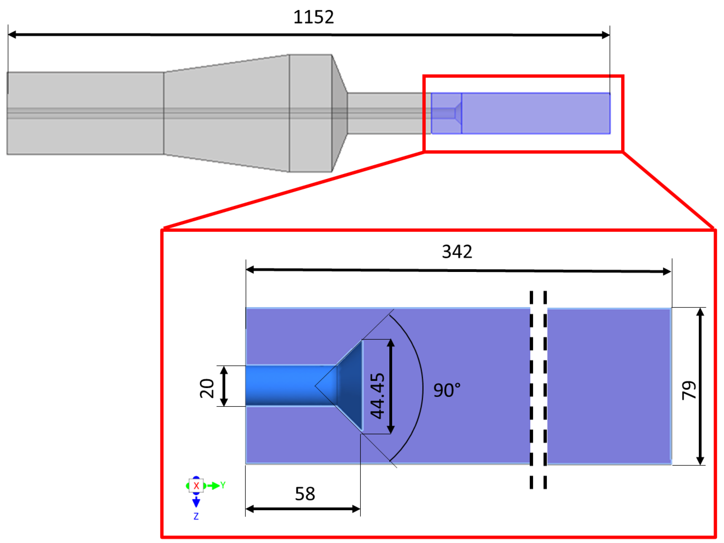
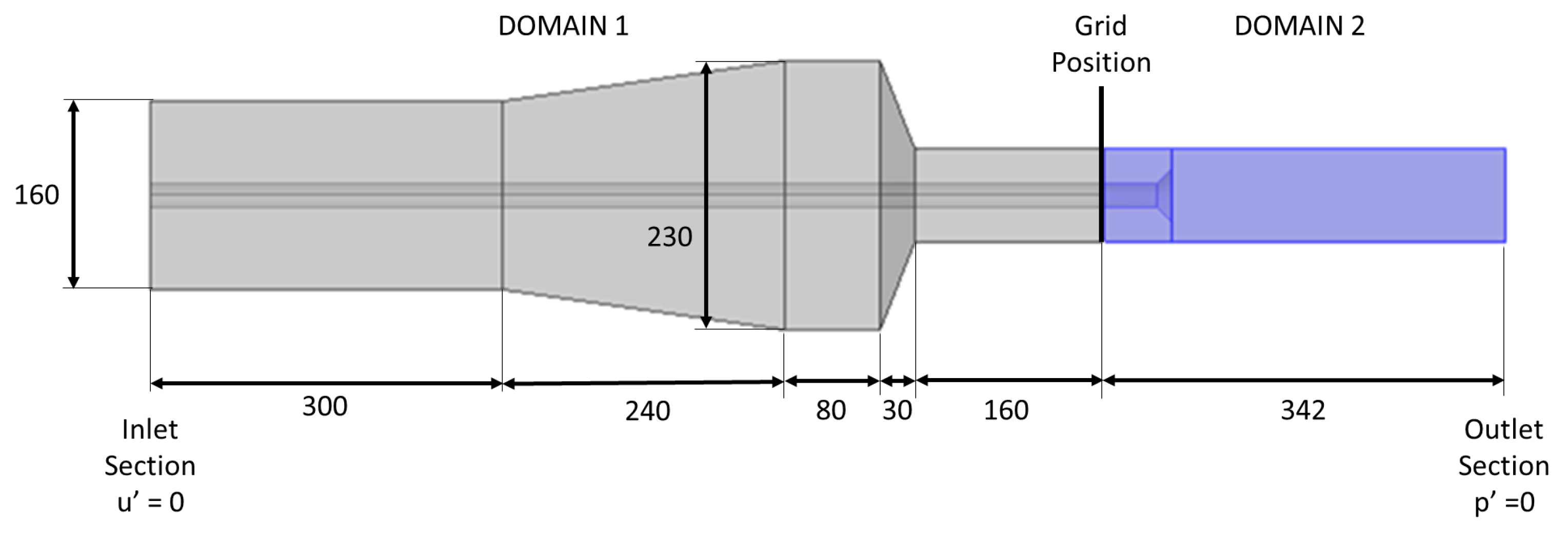
2. Combustor Geometry
3. Governing Equation and Numerical Setup
3.1. CFD Simulations
3.2. Thermoacoustic Combustion Instability Modelling
3.3. Thermoacoustic Numerical Setup
4. Results
4.1. Simulation of Combustion with CH4 and H2
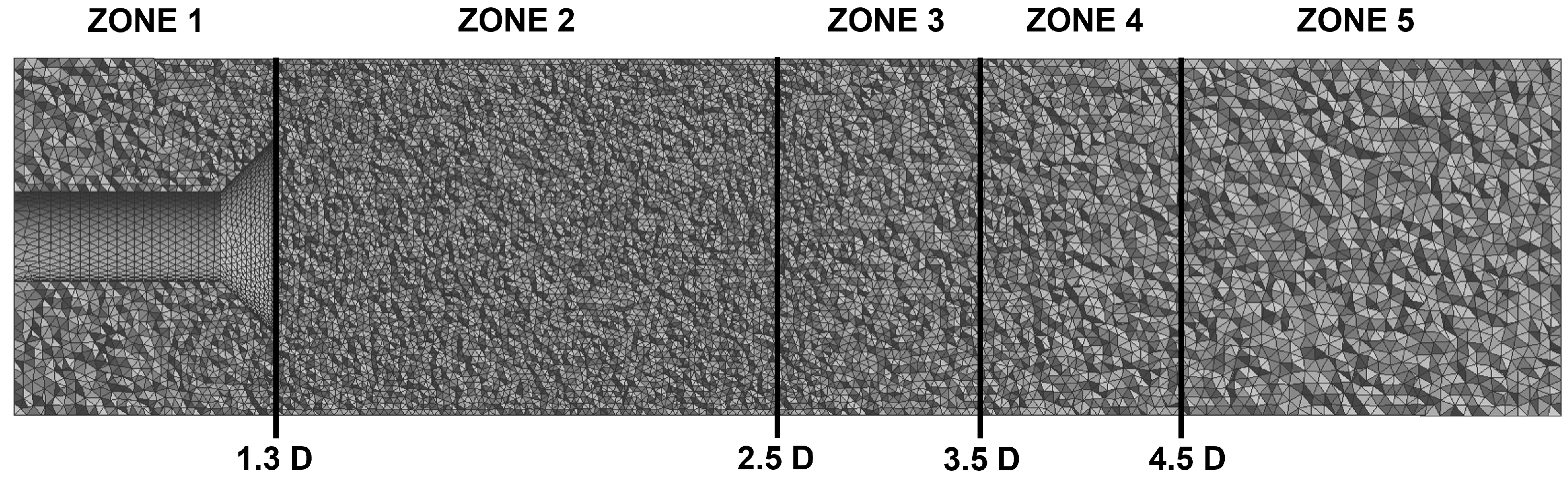
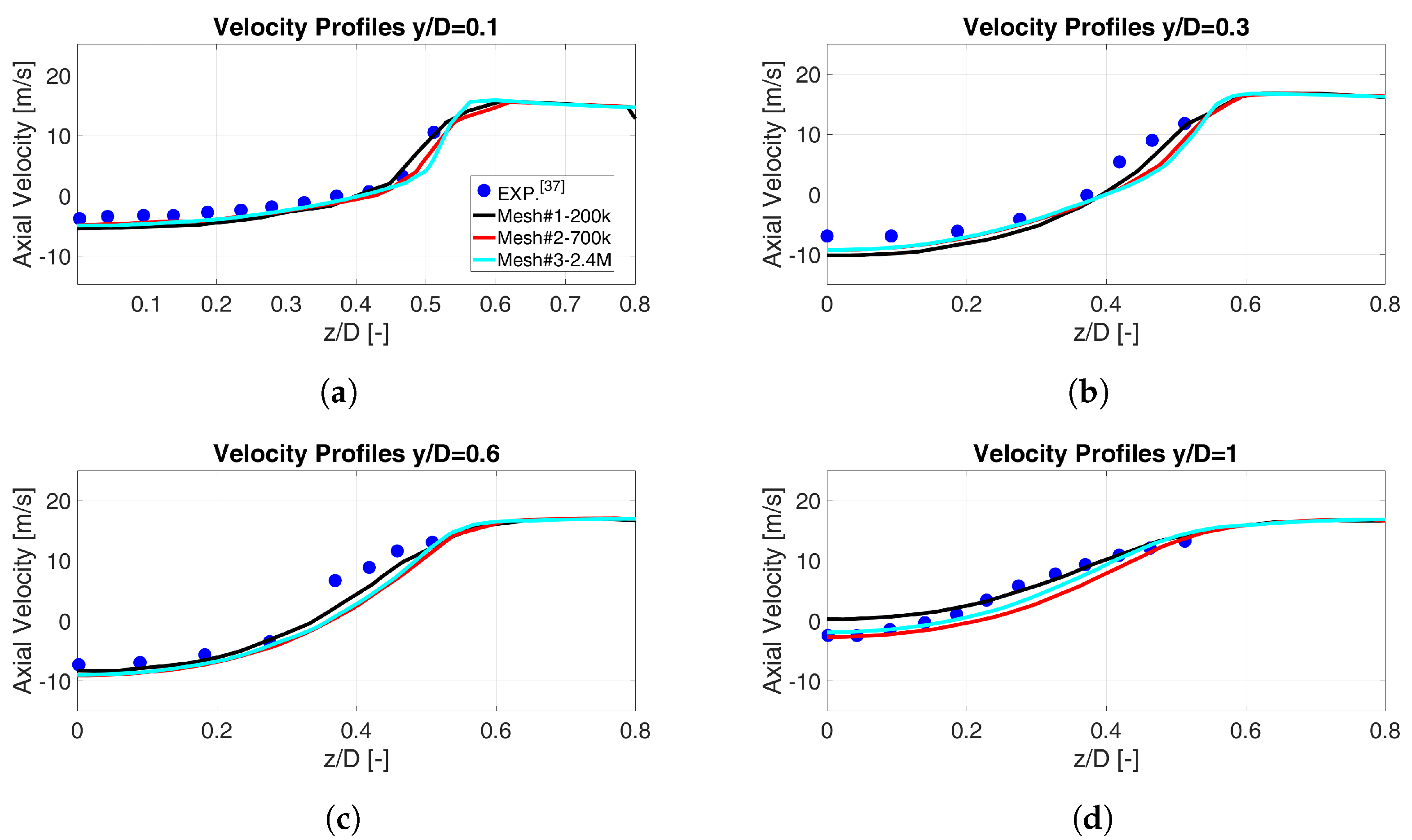
4.1.1. Grid Sensitivity Analysis of the RANS Simulations
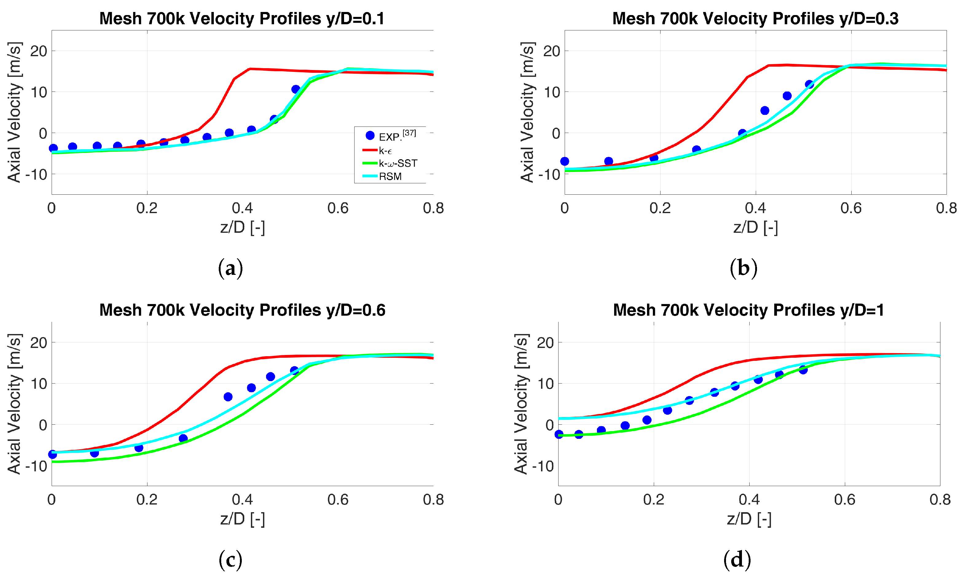
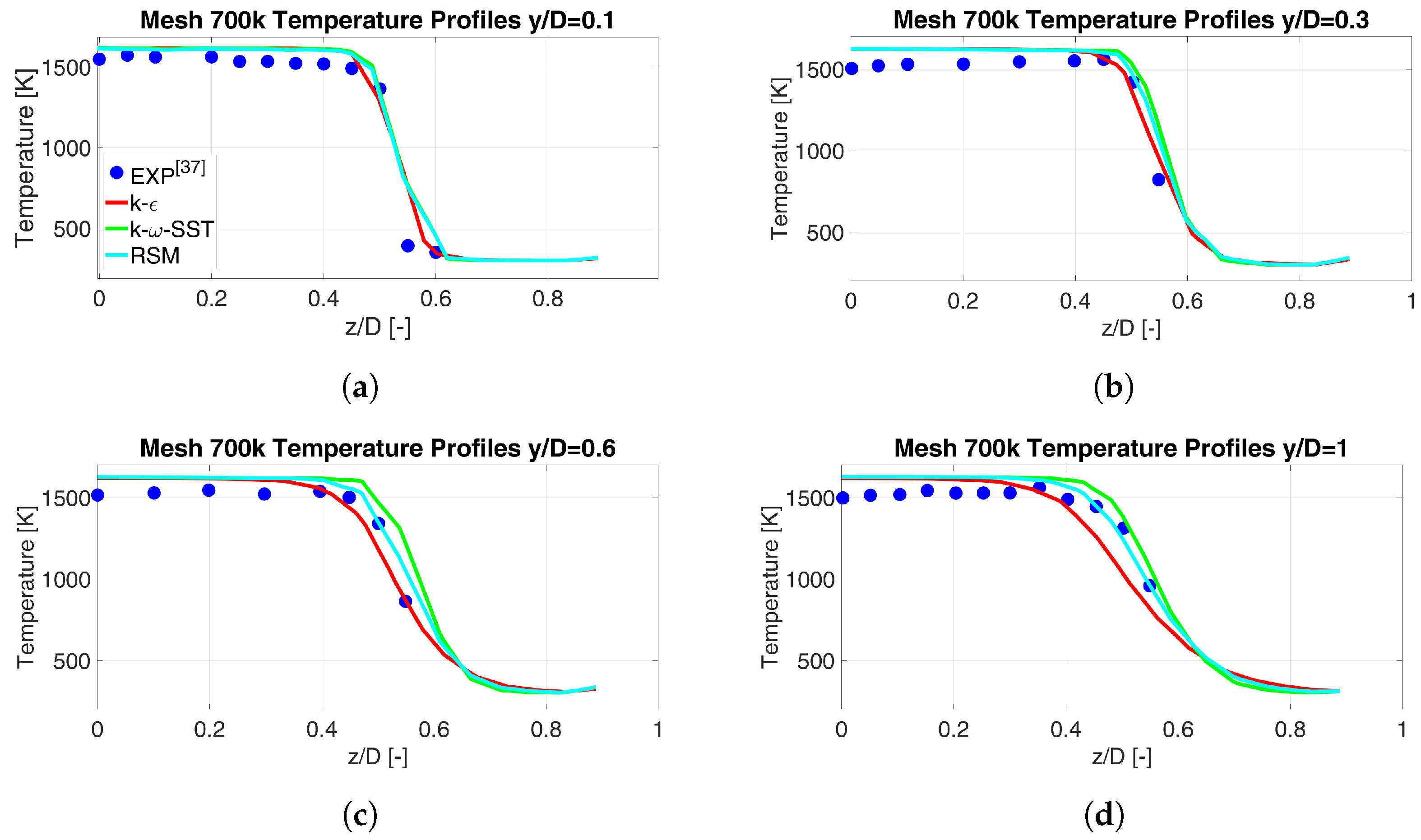
4.1.2. Turbulence Model Sensitivity Analysis of the RANS Simulations
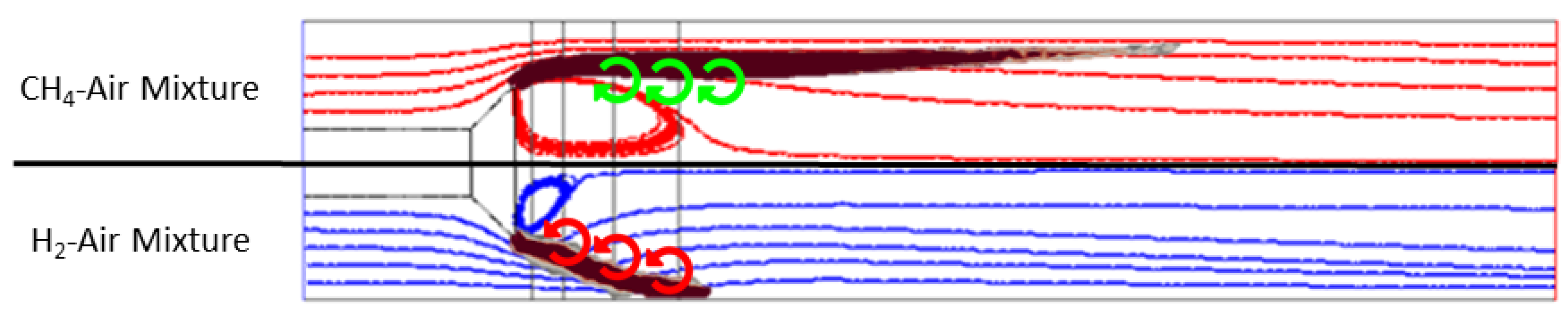
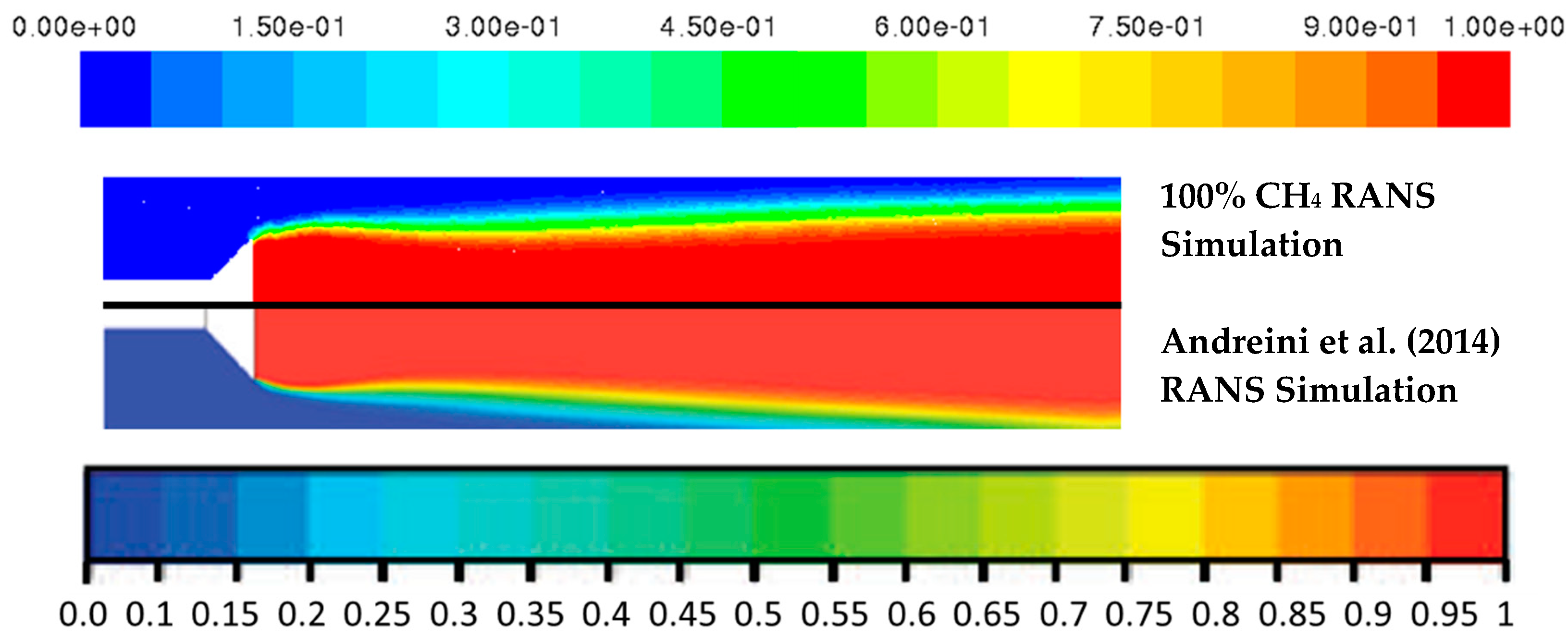
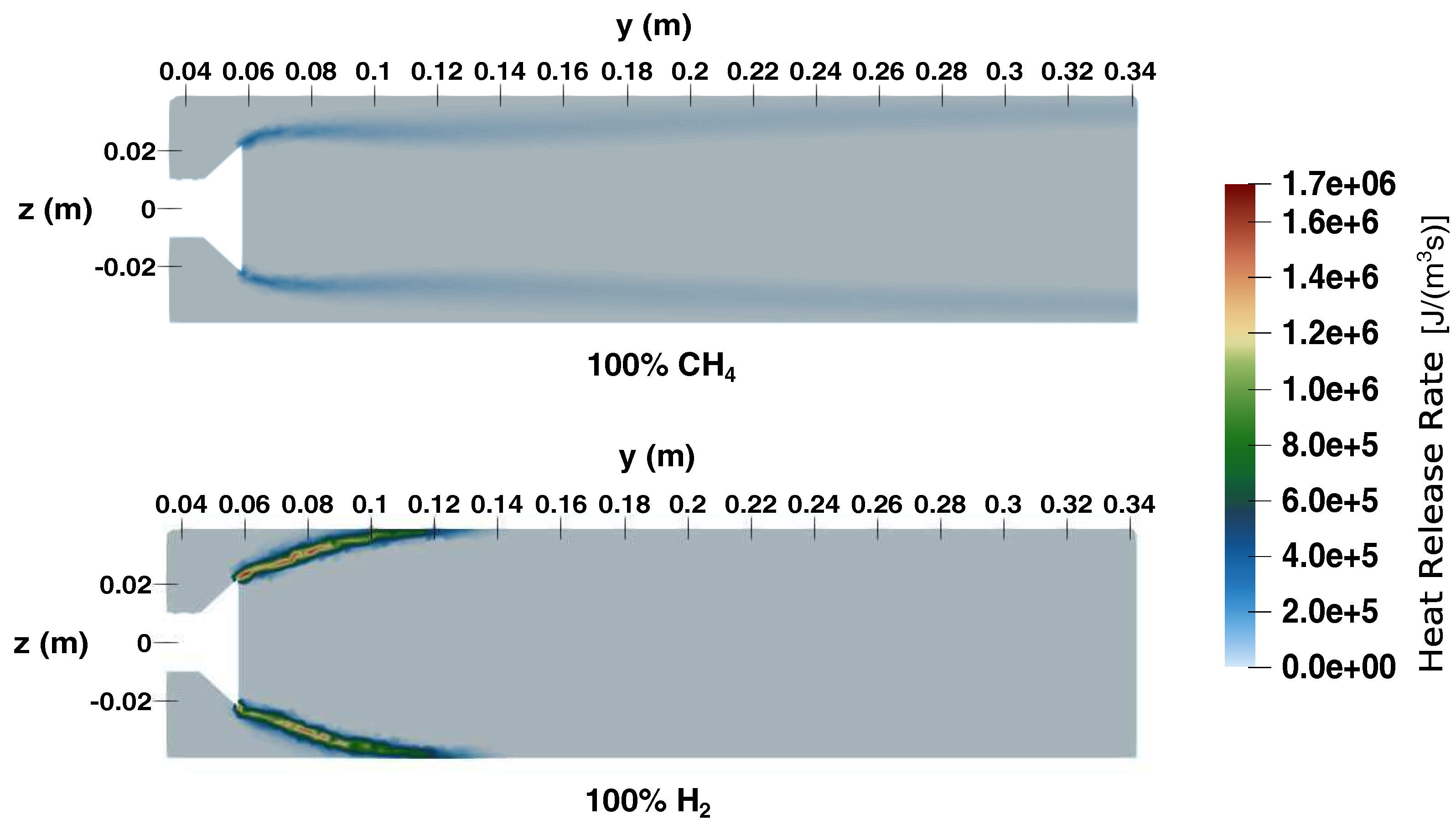
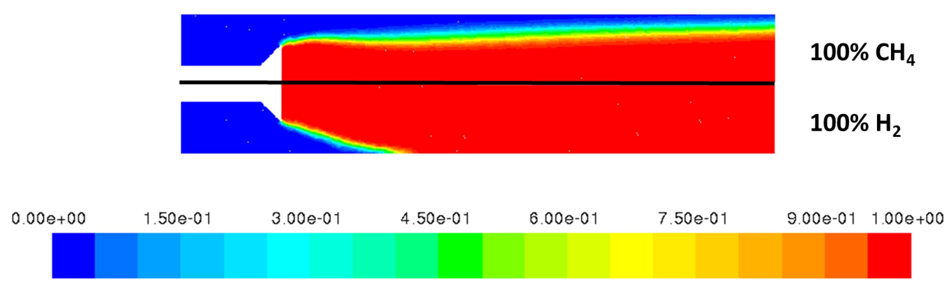
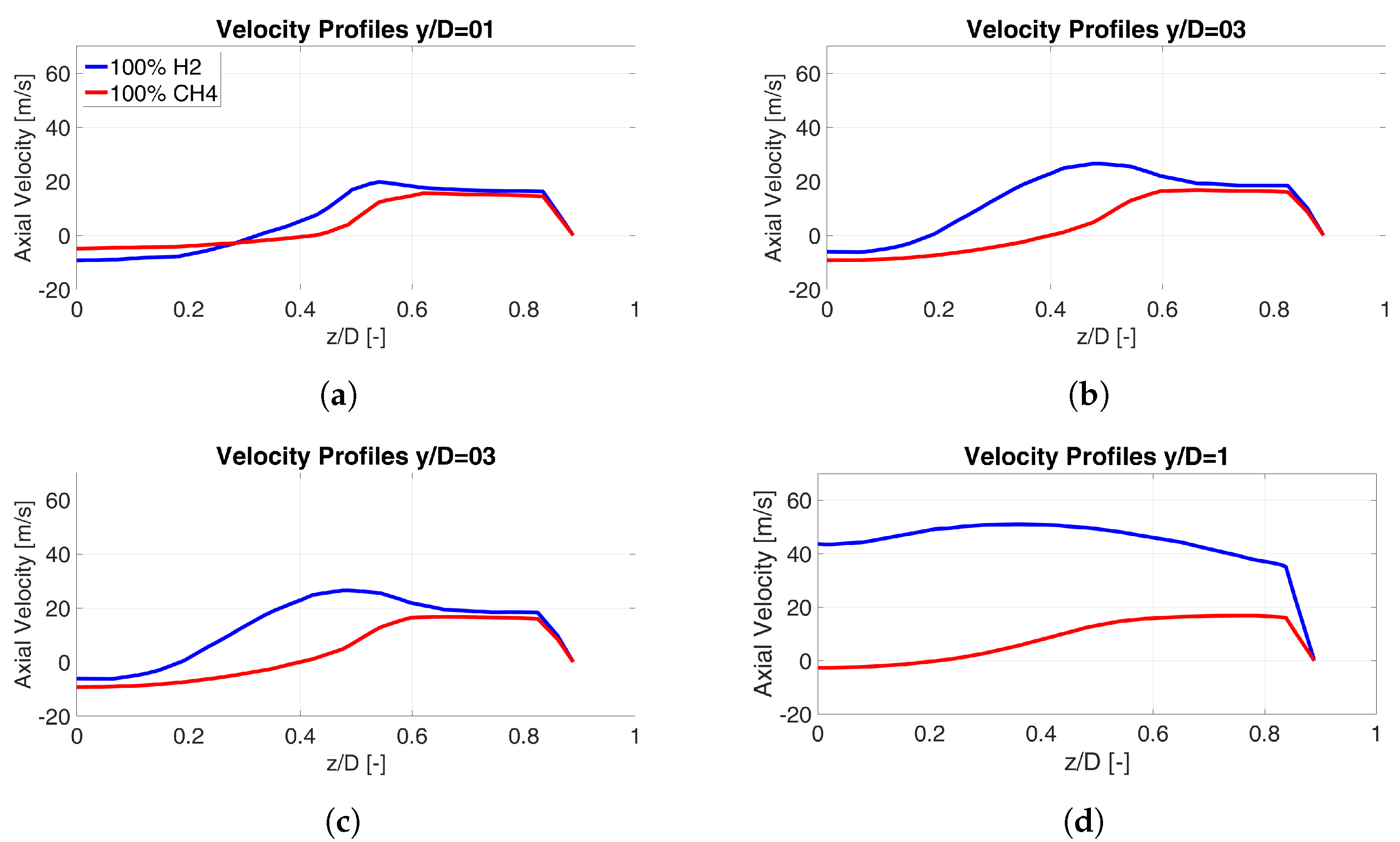
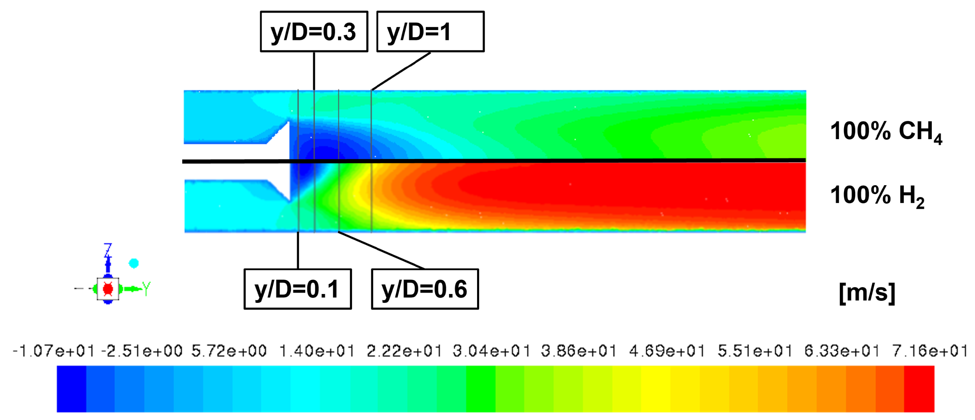
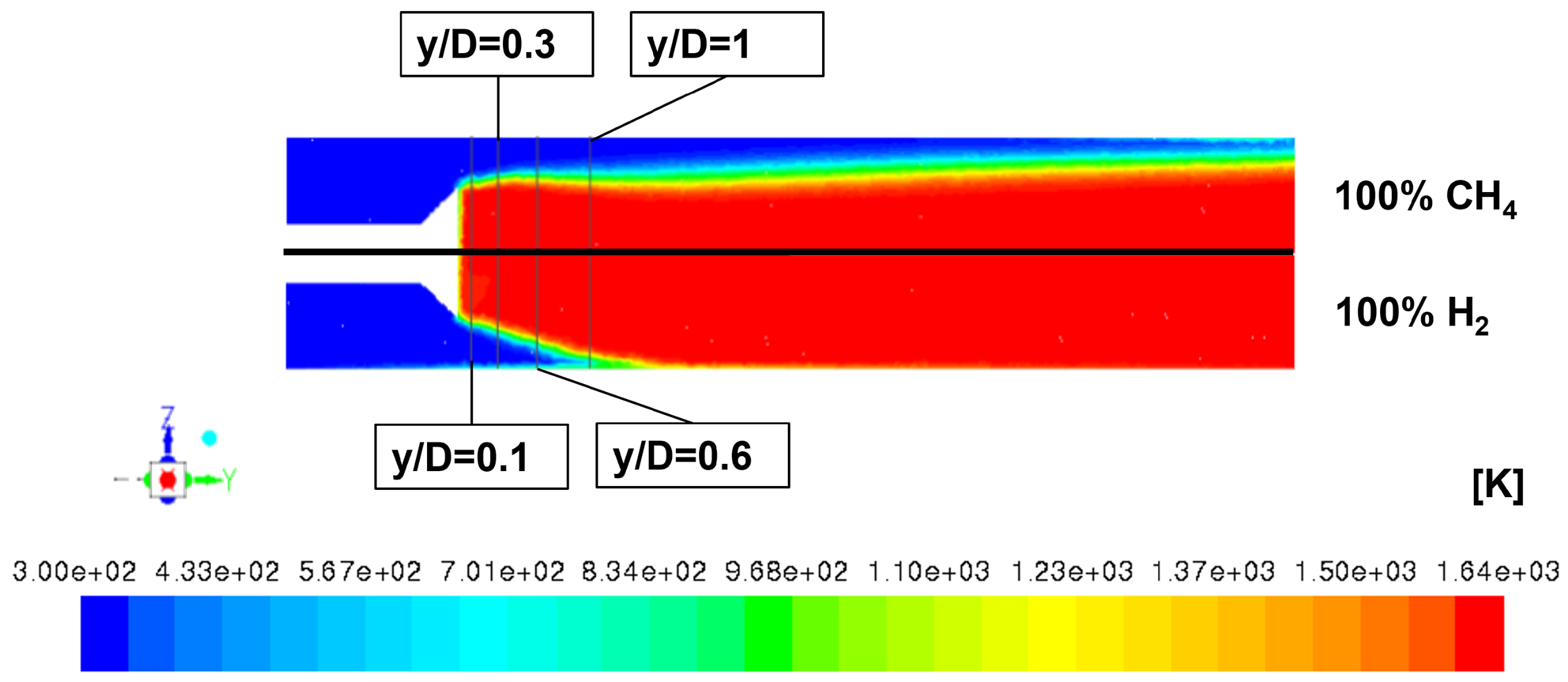
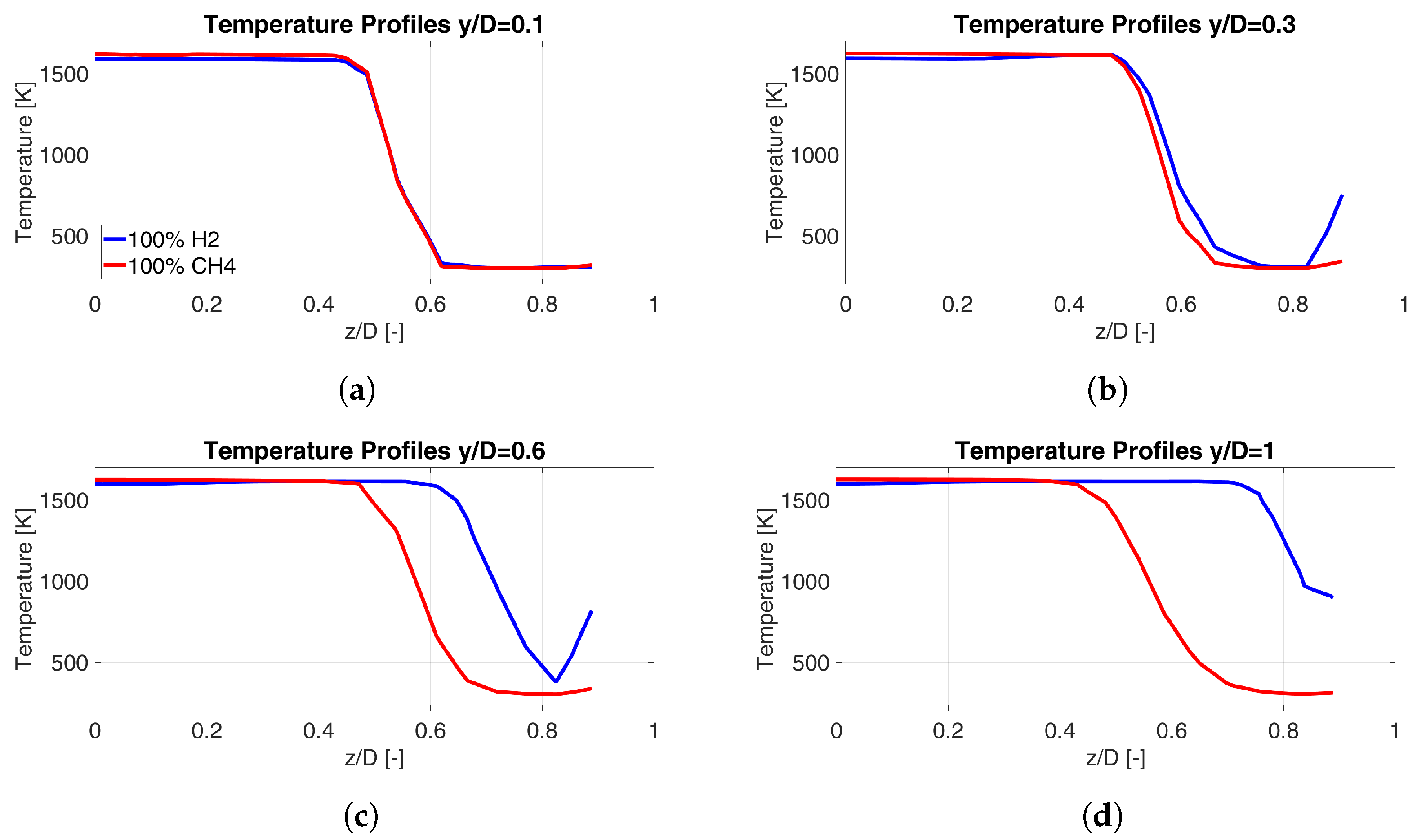
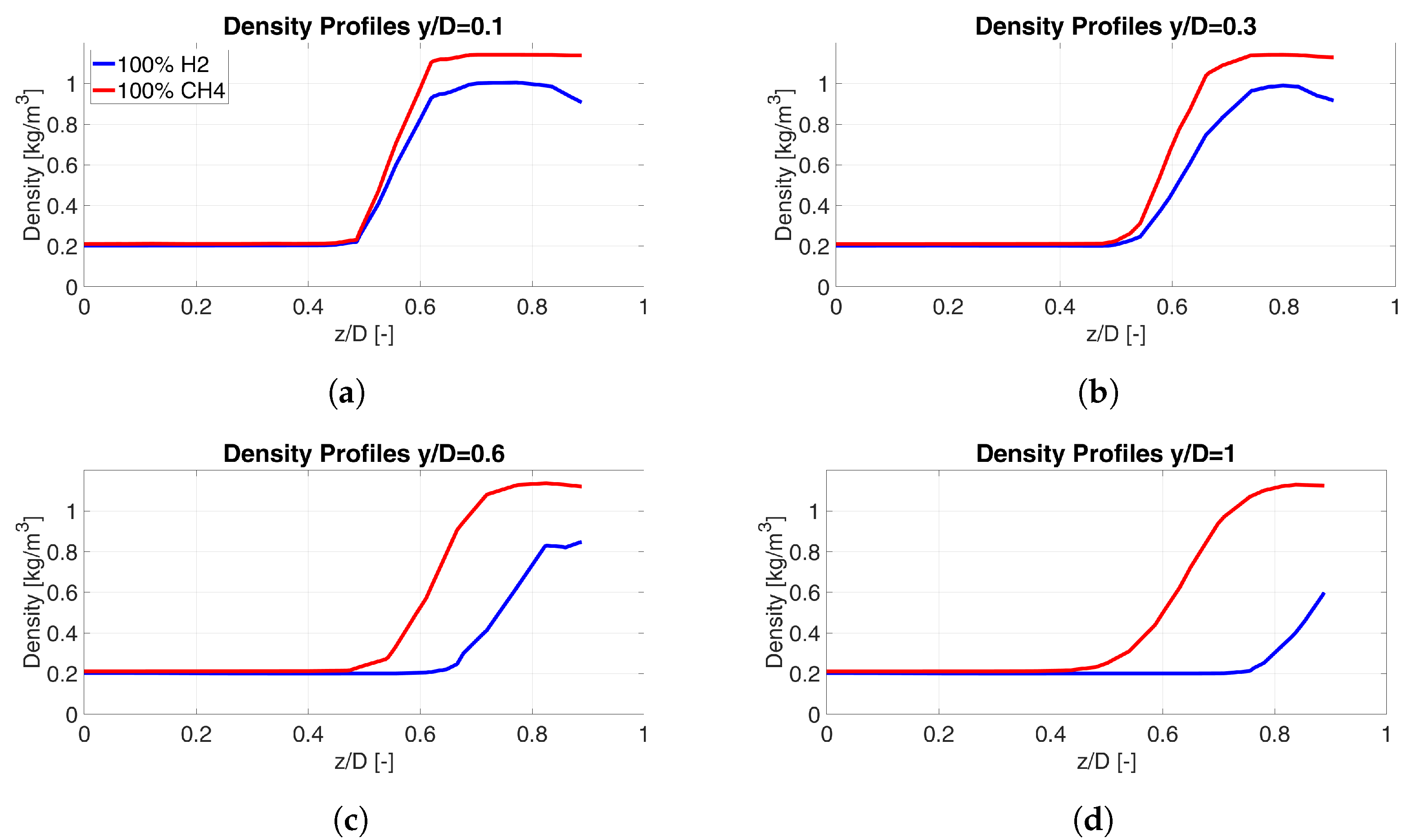
4.1.3. Results of the CFD Simulations
4.2. Influence of Fuel on the Thermoacoustics
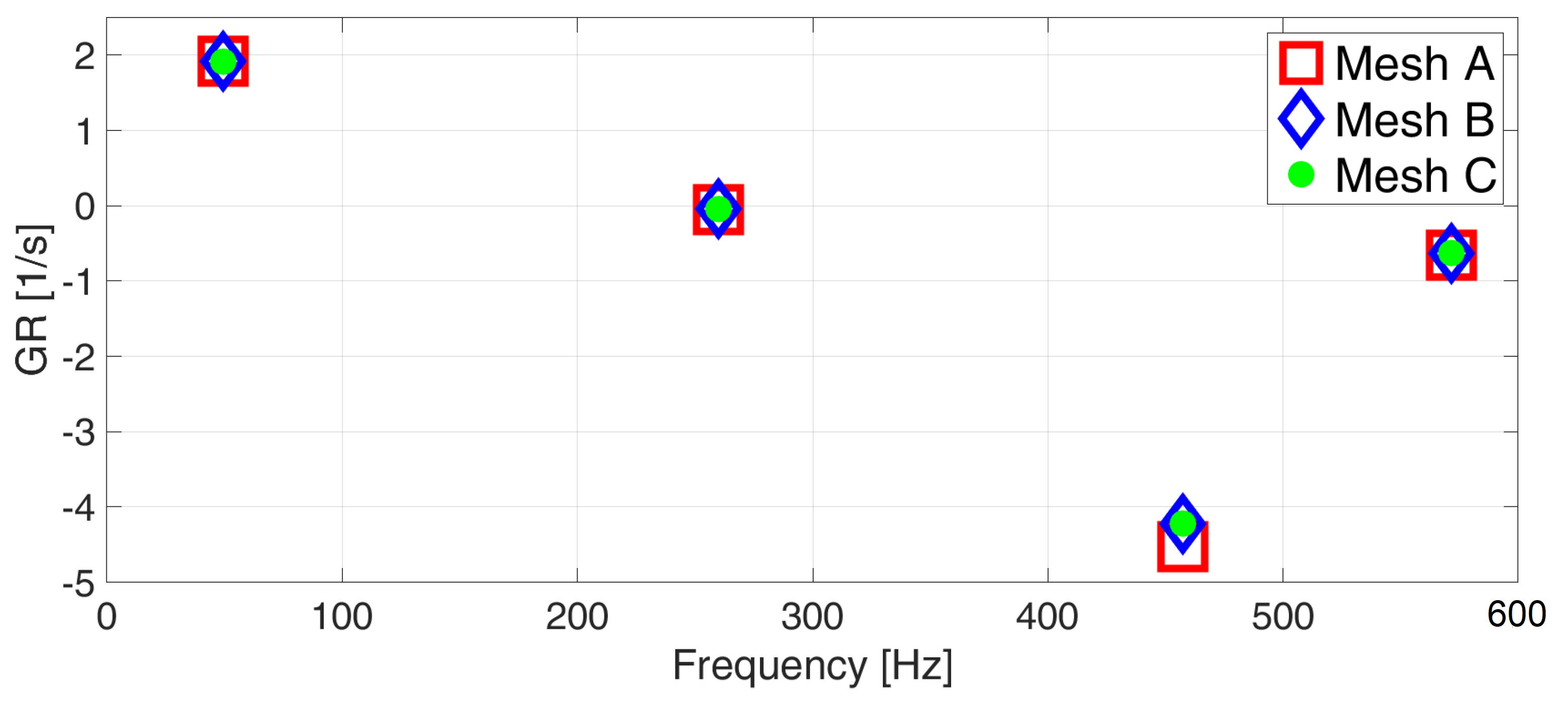
4.2.1. Grid Sensitivity Analysis of the Thermoacoustic Simulations
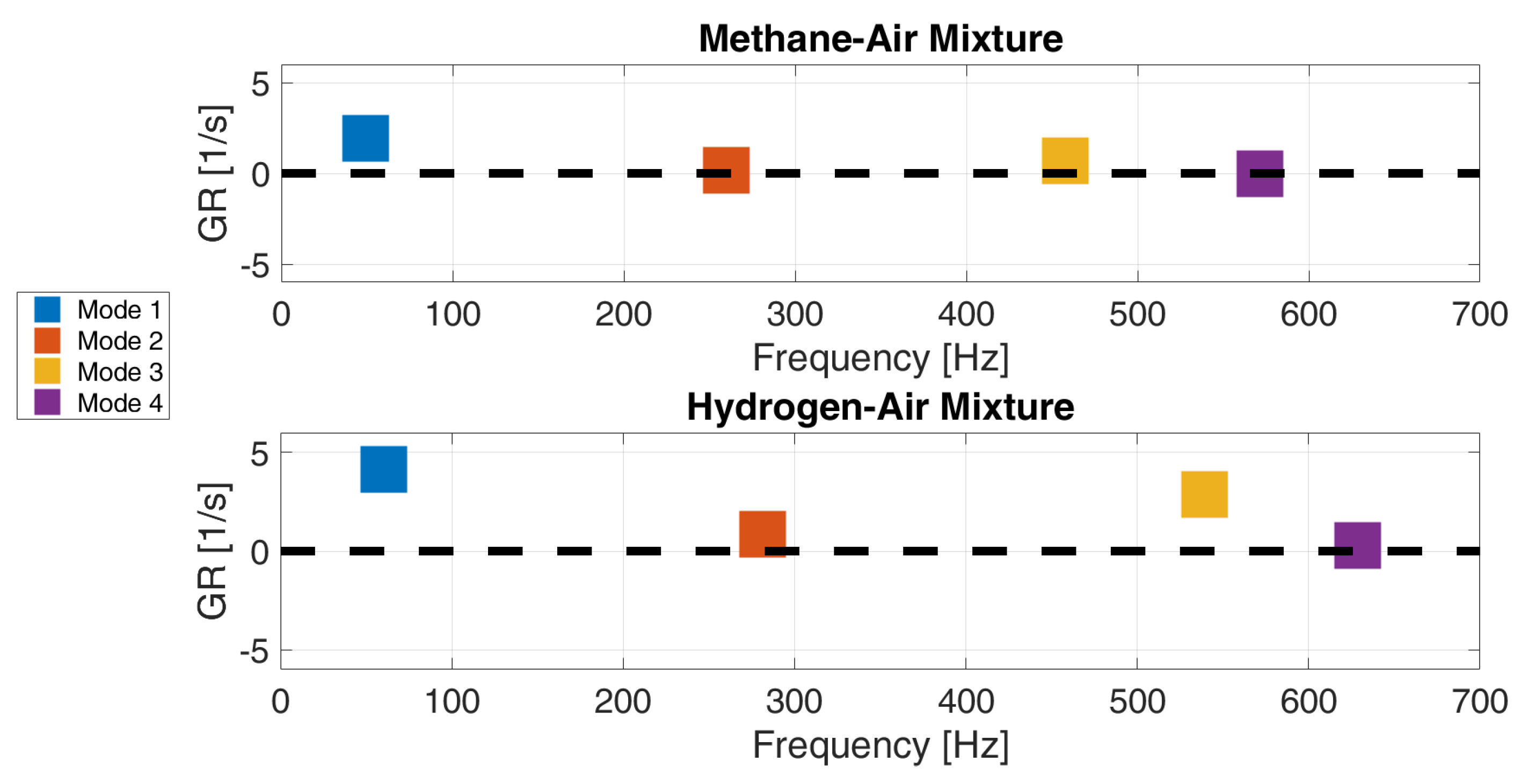
4.2.2. Results of the Thermoacoustic Simulations
5. Conclusions
Author Contributions
Funding
Data Availability Statement
Conflicts of Interest
Nomenclature
| Subscript | |
| Axial component | |
| Fuel mix | |
| Fuel | |
| j | Reference position |
| Air | |
| Stoichiometric | |
| Burner | |
| t | Turbulent |
| b | Burnt |
| u | Unburnt |
| l | Laminar |
| Superscript | |
| Mean | |
| Acoustic quantity | |
| Fluctuation | |
| m | Harmonic order |
| Greek letters | |
| Time delay | |
| Complex angular frequency | |
| Ratio between specific heat | |
| Density | |
| ∂ | Partial derivative |
| Fuel–air ratio | |
| Equivalence ratio | |
| Phase | |
| Progress variable | |
| Viscosity | |
| Symbols | |
| n | Acoustic–combustion interaction index |
| D | Bluff body max diameter |
| Diffusion coefficient | |
| T | Temperature |
| p | Pressure |
| u | Velocity |
| Bulk velocity | |
| P | Thermal power |
| y | y-coordinate |
| z | z-coordinate |
| Specific heat at constant pressure | |
| Specific heat at constant volume | |
| q | Heat release rate |
| c | Speed of sound |
| Molecular weight | |
| V | Control volume |
| f | Frequency |
| Spatial coordinate | |
| Real part | |
| Rayleigh index | |
| Wave energy dissipation | |
| Schmidt number | |
Abbreviations
| CFD | Computational fluid dynamics |
| FRF | Flame response function |
| RANS | Reynolds-averaged Navier–Stokes |
| FEM | Finite element method |
| GR | Growth rate |
| LHV | Lower heating value |
| FRF | Flame transfer function |
References
- Capurso, T.; Stefanizzi, M.; Torresi, M.; Camporeale, S. Perspective of the role of hydrogen in the 21st century energy transition. Energy Convers. Manag. 2022, 251, 114898. [Google Scholar] [CrossRef]
- Kovač, A.; Paranos, M.; Marciuš, D. Hydrogen in energy transition: A review. Int. J. Hydrogen Energy 2021, 46, 10016–10035. [Google Scholar] [CrossRef]
- International Renewable Energy Agency (IRENA). Hydrogen from Renewable Power: Technology Outlook for the Energy Transition. Abu Dhabi. 2018. Available online: https://www.irena.org/publications/2018/sep/hydrogen-from-renewable-power (accessed on 3 March 2023).
- Stefanizzi, M.; Capurso, T.; Filomeno, G.; Torresi, M.; Pascazio, G. Recent Combustion Strategies in Gas Turbines for Propulsion and Power Generation toward a Zero-Emissions Future: Fuels, Burners, and Combustion Techniques. Energies 2021, 14, 6694. [Google Scholar] [CrossRef]
- Griebel, P. Gas Turbines and Hydrogen. Hydrogen Science and Engineering: Materials, Processes, Systems and Technology; Wiley: Hoboken, NJ, USA, 2016; pp. 1011–1032. [Google Scholar]
- Stefanizzi, M.; Stefanizzi, S.; Ceglie, V.; Capurso, T.; Torresi, M.; Camporeale, S.M. Analysis of the partially premixed combustion in a labscale swirl-stabilized burner fueled by a methane-hydrogen mixture. E3S Web Conf. 2021, 312, 11004. [Google Scholar]
- Kutne, P. The Path Towards a Zero-Carbon Gas Turbine; Technical Report, European Turbine Network; ETN Global: Brussels, Belgium, 2020. [Google Scholar]
- Guiberti, T.F.; Durox, D.; Scouflaire, P.; Schuller, T. Impact of heat loss and hydrogen enrichment on the shape of confined swirling flames. Proc. Combust. Inst. 2015, 35, 1385–1392. [Google Scholar] [CrossRef]
- Kelsall, G.; Troger, C. Prediction and control of combustion instabilities in industrial gas turbines. Appl. Therm. Eng. 2004, 24, 1571–1582. [Google Scholar] [CrossRef]
- Chterev, I.; Boxx, I. Flame Topology and Combustion Instability Limits of Lean Premixed Hydrogen Enriched Flames. In Proceedings of the 27th International Colloquium on the Dynamics of Explosions and Reactive Systems (ICDERS), Beijing, China, 28 July–2 August 2019; Volume 28. [Google Scholar]
- Chterev, I.; Boxx, I. Effect of hydrogen enrichment on the dynamics of a lean technically premixed elevated pressure flame. Combust. Flame 2021, 225, 149–159. [Google Scholar] [CrossRef]
- Schefer, R.W.; Wicksall, D.; Agrawal, A.K. Combustion of hydrogen-enriched methane in a lean premixed swirl-stabilized burner. Proc. Combust. Inst. 2002, 29, 843–851. [Google Scholar] [CrossRef]
- Stow, S.R.; Dowling, A.P. Low-order modelling of thermoacoustic limit cycles. In Proceedings of the Turbo Expo: Power for Land, Sea, and Air, Perugia, Italy, 14–18 June 2004; Volume 41669, pp. 775–786. [Google Scholar]
- Evesque, S.P.; Polifke, W. Low-order acoustic modelling for annular combustors: Validation and inclusion of modal coupling. In Proceedings of the Turbo Expo: Power for Land, Sea, and Air, Amsterdam, The Netherlands, 3–6 June 2002; Volume 36061, pp. 321–331. [Google Scholar]
- Andreini, A.; Facchini, B.; Mangani, L.; Simonetti, F. Development and validation of a 1-D tool for thermoacoustic instabilities analysis in gas turbine combustors. In Proceedings of the Turbo Expo: Power for Land, Sea, and Air, Berlin, Germany, 9–13 June 2008; Volume 43130, pp. 951–960. [Google Scholar]
- Moin, P.; Apte, S.V. Large-eddy simulation of realistic gas turbine combustors. AIAA J. 2006, 44, 698–708. [Google Scholar] [CrossRef]
- Boudier, G.; Gicquel, L.; Poinsot, T.; Bissieres, D.; Bérat, C. Comparison of LES, RANS and experiments in an aeronautical gas turbine combustion chamber. Proc. Combust. Inst. 2007, 31, 3075–3082. [Google Scholar] [CrossRef]
- Sengissen, A.; Van Kampen, J.; Huls, R.; Stoffels, G.G.; Kok, J.B.; Poinsot, T. LES and experimental studies of cold and reacting flow in a swirled partially premixed burner with and without fuel modulation. Combust. Flame 2007, 150, 40–53. [Google Scholar] [CrossRef]
- Staffelbach, G.; Gicquel, L.; Boudier, G.; Poinsot, T. Large Eddy Simulation of self excited azimuthal modes in annular combustors. Proc. Combust. Inst. 2009, 32, 2909–2916. [Google Scholar] [CrossRef] [Green Version]
- Wolf, P.; Balakrishnan, R.; Staffelbach, G.; Gicquel, L.Y.; Poinsot, T. Using LES to study reacting flows and instabilities in annular combustion chambers. Flow Turbul. Combust. 2012, 88, 191–206. [Google Scholar] [CrossRef] [Green Version]
- Nicoud, F.; Benoit, L.; Sensiau, C.; Poinsot, T. Acoustic modes in combustors with complex impedances and multidimensional active flames. AIAA J. 2007, 45, 426–441. [Google Scholar] [CrossRef] [Green Version]
- Camporeale, S.; Fortunato, B.; Campa, G. A finite element method for three-dimensional analysis of thermo-acoustic combustion instability. J. Eng. Gas Turbines Power 2011, 133, 011506. [Google Scholar] [CrossRef]
- Laera, D.; Camporeale, S.M. A weakly nonlinear approach based on a distributed flame describing function to study the combustion dynamics of a full-scale lean-premixed swirled burner. J. Eng. Gas Turbines Power 2017, 139, 091501. [Google Scholar] [CrossRef]
- Ceglie, V.; Capurso, T.; Oresta, P.; Camporeale, S.M. Analysis of the Influence of the Mean Flow Field Mach Number on Thermo-Acoustic Combustion Instability. Edp Sci. 2020, 197, 11004. [Google Scholar] [CrossRef]
- Laera, D.; Agostinelli, P.W.; Selle, L.; Cazères, Q.; Oztarlik, G.; Schuller, T.; Gicquel, L.; Poinsot, T. Stabilization mechanisms of CH4 premixed swirled flame enriched with a non-premixed hydrogen injection. Proc. Combust. Inst. 2021, 38, 6355–6363. [Google Scholar] [CrossRef]
- Crocco, L.; Cheng, S.I. Theory of Combustion Instability in Liquid Propellant Rocket Motors; Technical Report; Princeton University: Princeton, NJ, USA, 1956. [Google Scholar]
- Laera, D.; Camporeale, S.M. Numerical and experimental studies on self sustained thermo-acoustic combustion instabilities of an experimental rig for full-scale industrial burners. Int. J. Gas Turbine, Propuls. Power Syst. 2017, 9, 37–46. [Google Scholar]
- Beita, J.; Talibi, M.; Sadasivuni, S.; Balachandran, R. Thermoacoustic Instability Considerations for High Hydrogen Combustion in Lean Premixed Gas Turbine Combustors: A Review. Hydrogen 2021, 2, 33–57. [Google Scholar] [CrossRef]
- Janus, M.C.; Richards, G.A.; Yip, M.J.; Robey, E.H. Effects of ambient conditions and fuel composition on combustion stability. In Proceedings of the Turbo Expo: Power for Land, Sea, and Air, Orlando, FL, USA, 2–5 June 1997; American Society of Mechanical Engineers: New York, NY, USA, 1997; Volume 78699, p. V002T06A035. [Google Scholar]
- Æsøy, E.; Aguilar, J.G.; Wiseman, S.; Bothien, M.R.; Worth, N.A.; Dawson, J.R. Scaling and prediction of transfer functions in lean premixed H2/CH4-flames. Combust. Flame 2020, 215, 269–282. [Google Scholar] [CrossRef]
- Aguilar, J.G.; Æsøy, E.; Dawson, J.R. The influence of hydrogen on the stability of a perfectly premixed combustor. Combust. Flame 2022, 245, 112323. [Google Scholar] [CrossRef]
- Shanbhogue, S.; Sanusi, Y.; Taamallah, S.; Habib, M.; Mokheimer, E.; Ghoniem, A. Flame macrostructures, combustion instability and extinction strain scaling in swirl-stabilized premixed CH4/H2 combustion. Combust. Flame 2016, 163, 494–507. [Google Scholar] [CrossRef]
- Ahn, B.; Indlekofer, T.; Dawson, J.; Worth, N. Transient Thermo-Acoustic Responses of Methane/Hydrogen Flames in a Pressurized Annular Combustor. J. Eng. Gas Turbines Power 2022, 144, 14. [Google Scholar] [CrossRef]
- Veiga-López, F.; Martınez-Ruiz, D.; Kuznetsov, M.; Sánchez-Sanz, M. Thermoacoustic analysis of lean H2-air premixed flames in thin layers. In Proceedings of the 27th International Colloquium on the Dynamics of Explosions and Reactive Systems (ICDERS 2019), Beijing, China, 28 July–2 August 2019. [Google Scholar]
- Kim, Y.J.; Yoon, Y.; Lee, M.C. On the observation of high-order, multi-mode, thermo-acoustic combustion instability in a model gas turbine combustor firing hydrogen containing syngases. Int. J. Hydrogen Energy 2019, 44, 11111–11120. [Google Scholar] [CrossRef]
- Pan, J.; Vangsness, M.; Ballal, D. Aerodynamics of bluff-body stabilized confined turbulent premixed flames. J. Eng. Gas Turbines Power 1992, 114, 783–789. [Google Scholar] [CrossRef]
- Nandula, S.; Pitz, R.; Barlow, R.; Fiechtner, G. Rayleigh/Raman/LIF measurements in a turbulent lean premixed combustor. In Proceedings of the 34th Aerospace Sciences Meeting and Exhibit, Reno, NV, USA, 15–18 January 1996; p. 937. [Google Scholar]
- Cannon, S.; Brewster, B.; Smoot, L. PDF modeling of lean premixed combustion using in situ tabulated chemistry. Combust. Flame 1999, 119, 233–252. [Google Scholar] [CrossRef]
- Andreini, A.; Bianchini, C.; Innocenti, A. Large eddy simulation of a bluff body stabilized lean premixed flame. J. Combust. 2014, 2014, 710254. [Google Scholar] [CrossRef] [Green Version]
- Sudarma, A. RANS numerical simulation of lean premixed bluff body stabilized combustor: Comparison of turbulence models. J. Therm. Eng. 2017, 3, 1561–1573. [Google Scholar] [CrossRef]
- Ansys Fluent Theory Guide; ANSYS, Inc.: Canonsburg, PA, USA, 2022; Available online: http://www.pmt.usp.br/academic/martoran/notasmodelosgrad/ANSYS%20Fluent%20Theory%20Guide%2015.pdf (accessed on 3 March 2023).
- Smith, G.P. GRI-Mech 3.0. 1999. Available online: http://combustion.berkeley.edu/gri-mech/version30/text30.html (accessed on 3 March 2023).
- Zimont, V.; Polifke, W.; Bettelini, M.; Wolfgang, W. An efficient computational model for premixed turbulent combustion at high Reynolds numbers based on a turbulent flame speed closure. J. Eng. Gas Turbines Power 1998, 120, 526–532. [Google Scholar] [CrossRef]
- Rayleigh, J.W.S.B. The Theory of Sound; Macmillan & Company: New York, NY, USA, 1896; Volume 2. [Google Scholar]
- Lieuwen, T.C.; Yang, V. Combustion Instabilities in Gas Turbine Engines: Operational Experience, Fundamental Mechanisms, and Modeling; American Institute of Aeronautics and Astronautics: Reston, VA, USA, 2005. [Google Scholar]
- Hermeth, S.; Staffelbach, G.; Gicquel, L.Y.; Anisimov, V.; Cirigliano, C.; Poinsot, T. Bistable swirled flames and influence on flame transfer functions. Combust. Flame 2014, 161, 184–196. [Google Scholar] [CrossRef] [Green Version]
- Schadow, K.; Gutmark, E. Combustion instability related to vortex shedding in dump combustors and their passive control. Prog. Energy Combust. Sci. 1992, 18, 117–132. [Google Scholar] [CrossRef]
- Poinsot, T.J.; Trouve, A.C.; Veynante, D.P.; Candel, S.M.; Esposito, E.J. Vortex-driven acoustically coupled combustion instabilities. J. Fluid Mech. 1987, 177, 265–292. [Google Scholar] [CrossRef]
- Matveev, K.I.; Culick, F. A model for combustion instability involving vortex shedding. Combust. Sci. Technol. 2003, 175, 1059–1083. [Google Scholar] [CrossRef]
- Durox, D.; Schuller, T.; Candel, S. Combustion dynamics of inverted conical flames. Proc. Combust. Inst. 2005, 30, 1717–1724. [Google Scholar] [CrossRef]
- Gatti, M.; Gaudron, R.; Mirat, C.; Zimmer, L.; Schuller, T. Impact of swirl and bluff-body on the transfer function of premixed flames. Proc. Combust. Inst. 2019, 37, 5197–5204. [Google Scholar] [CrossRef]
- Campa, G.; Camporeale, S.M. Prediction of the thermoacoustic combustion instabilities in practical annular combustors. J. Eng. Gas Turbines Power 2014, 136, 091504. [Google Scholar] [CrossRef]
- Alemela, P.; Fanaca, D.; Hirsch, C.; Sattelmayer, T.; Schuermans, B. Determination and scaling of thermo acoustic characteristics of premixed flames. Int. J. Spray Combust. Dyn. 2010, 2, 169–198. [Google Scholar] [CrossRef] [Green Version]
- Dowling, A.P. Nonlinear self-excited oscillations of a ducted flame. J. Fluid Mechs. 1997, 346, 271–290. [Google Scholar] [CrossRef]
- Li, J.; Morgans, A.S. Time domain simulations of nonlinear thermoacoustic behaviour in a simple combustor using a wave-based approach. J. Sound Vib. 2015, 346, 345–360. [Google Scholar] [CrossRef] [Green Version]
- Menter, F.R. Two-equation eddy-viscosity turbulence models for engineering applications. AIAA J. 1994, 32, 1598–1605. [Google Scholar] [CrossRef] [Green Version]
- Lo Schiavo, E.; Laera, D.; Riber, E.; Gicquel, L.; Poinsot, T. On the impact of fuel injection angle in Euler–Lagrange large eddy simulations of swirling spray flames exhibiting thermoacoustic instabilities. Combust. Flame 2021, 227, 359–370. [Google Scholar] [CrossRef]
- Magri, L.; Juniper, M.P.; Moeck, J.P. Sensitivity of the Rayleigh criterion in thermoacoustics. J. Fluid Mech. 2020, 882, R1. [Google Scholar] [CrossRef] [Green Version]


| Parameter | CH4-Air | H2-Air |
|---|---|---|
| (−) | 0.586 | 0.481 |
| (−) | 17.20 | 33.9 |
| (Kg/kmol) | 28.11 | 24.31 |
| (−) | 29.30 | 70.6 |
| (g/s) | 70.78 | 70.78 |
| (g/s) | 2.42 | 1 |
| (Kg/m) | 1.14 | 0.99 |
| (m/s) | 10.81 | 12.26 |
| (MJ/Kg) | 50.0 | 119.9 |
| (K) | 1641 | 1577 |
| Zone | Stream Direction | Mesh #1 | Mesh #2 | Mesh #3 |
|---|---|---|---|---|
| ZONE 1 | 0–1.3D | 4.5 mm | 3 mm | 3 mm |
| ZONE 2 | 1.3D–2.5D | 4.5 mm | 3 mm | 1.6 mm |
| ZONE 3 | 2.5D–3.5D | 4.5 mm | 3 mm | 2 mm |
| ZONE 4 | 3.5D–4.5D | 4.5 mm | 3 mm | 2.5 mm |
| ZONE 5 | 4.5D–7.7D | 4.5 mm | 3 mm | 3 mm |
| N. of elements | 200 k | 700 k | 2.4 M |
| Domain | Parameter | Mesh A | Mesh B | Mesh C |
|---|---|---|---|---|
| Max element size | 92 mm | 63.4 mm | 40.3 mm | |
| Domain 1 | ||||
| (upstream of grid) | Min element size | 11.5 mm | 4.61 mm | 1.73 mm |
| Max element growth rate | 1.45 | 1.4 | 1.35 | |
| Max element size | 40.3 mm | 23 mm | 23 mm | |
| Domain 2 | ||||
| (downstream of grid) | Min element size | 1.73 mm | 0.24 mm | 0.24 mm |
| Max element growth rate | 1.35 | 1.3 | 1.3 | |
| Number of elements (-) | 31 k | 123 k | 255 k | |
| Computation time (s) | 64 | 332 | 623 | |
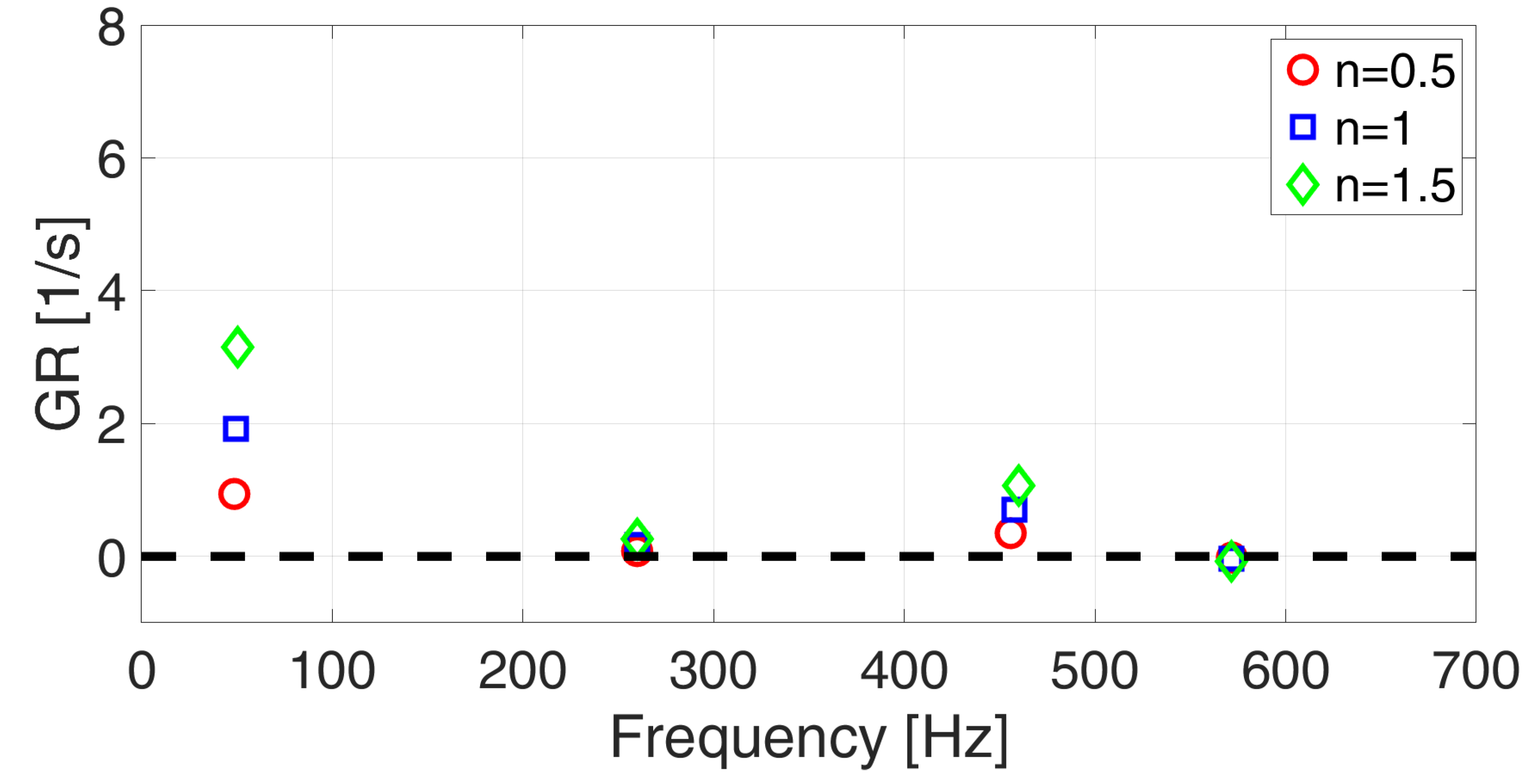
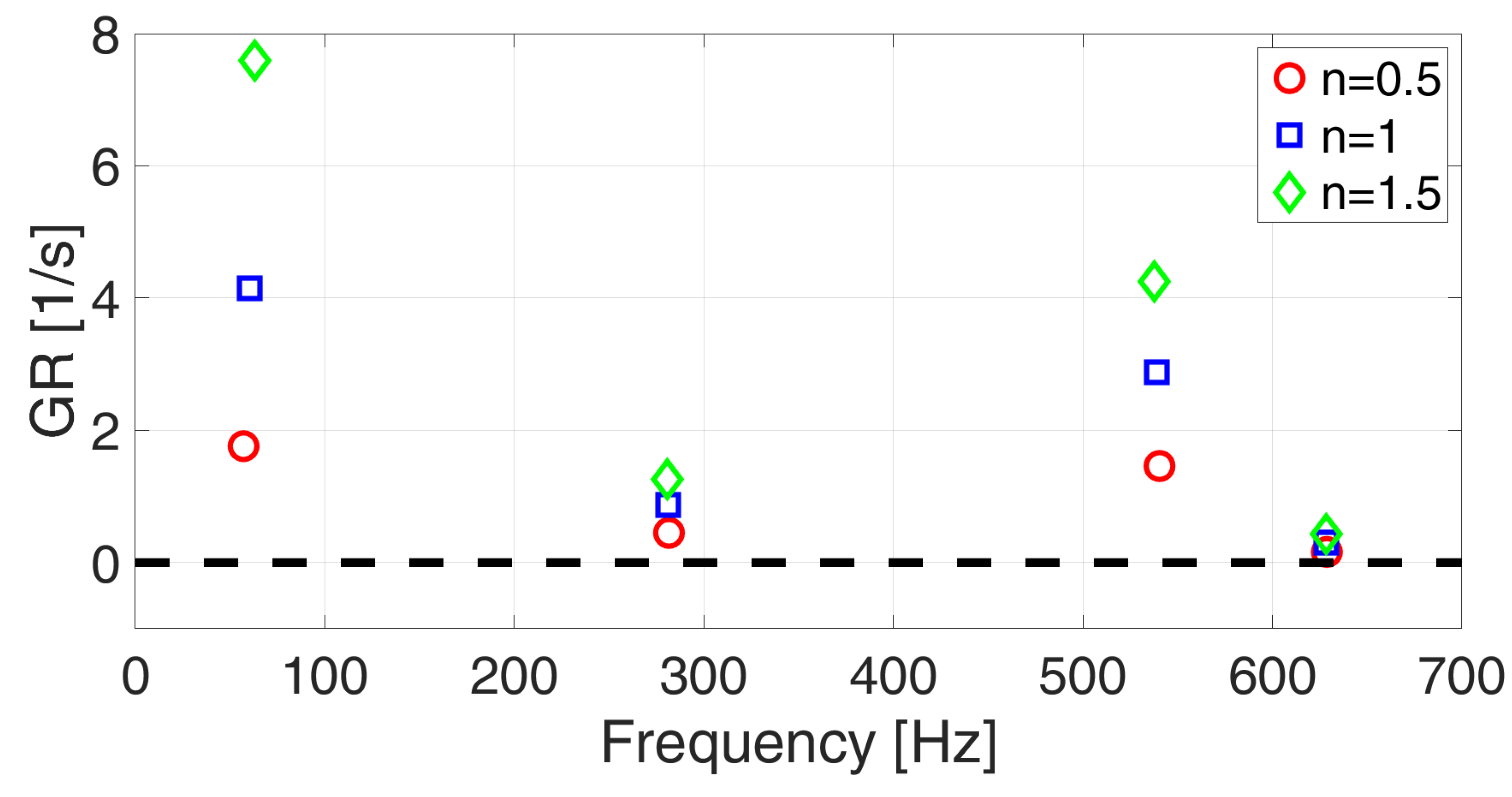
| Mode Type | CH4 with No Flame | CH4 with Flame | H2 with No Flame | H2 with Flame |
|---|---|---|---|---|
| Longitudinal | 47.68 Hz | 49.44 + 1.99i Hz | 54.18 Hz | 60.11 + 4.15i Hz |
| Longitudinal | 259.73 Hz | 259.96 + 0.17i Hz | 281.89 Hz | 281.21 + 0.87i Hz |
| Longitudinal | 453.87 Hz | 457.74 + 0.70i Hz | 541.78 Hz | 539.06 + 2.88i Hz |
| Longitudinal | 571.88 Hz | 571.65 − 0.038i Hz | 628.95 Hz | 628.48 + 0.30i Hz |
Disclaimer/Publisher’s Note: The statements, opinions and data contained in all publications are solely those of the individual author(s) and contributor(s) and not of MDPI and/or the editor(s). MDPI and/or the editor(s) disclaim responsibility for any injury to people or property resulting from any ideas, methods, instructions or products referred to in the content. |
© 2023 by the authors. Licensee MDPI, Basel, Switzerland. This article is an open access article distributed under the terms and conditions of the Creative Commons Attribution (CC BY) license (https://creativecommons.org/licenses/by/4.0/).
Share and Cite
Ceglie, V.; Stefanizzi, M.; Capurso, T.; Fornarelli, F.; Camporeale, S.M. Thermoacoustic Combustion Stability Analysis of a Bluff Body-Stabilized Burner Fueled by Methane–Air and Hydrogen–Air Mixtures. Energies 2023, 16, 3272. https://doi.org/10.3390/en16073272
Ceglie V, Stefanizzi M, Capurso T, Fornarelli F, Camporeale SM. Thermoacoustic Combustion Stability Analysis of a Bluff Body-Stabilized Burner Fueled by Methane–Air and Hydrogen–Air Mixtures. Energies. 2023; 16(7):3272. https://doi.org/10.3390/en16073272
Chicago/Turabian StyleCeglie, Vito, Michele Stefanizzi, Tommaso Capurso, Francesco Fornarelli, and Sergio M. Camporeale. 2023. "Thermoacoustic Combustion Stability Analysis of a Bluff Body-Stabilized Burner Fueled by Methane–Air and Hydrogen–Air Mixtures" Energies 16, no. 7: 3272. https://doi.org/10.3390/en16073272