Heat Transfer Analysis of Sisko Fluid Flow over a Stretching Sheet in a Conducting Field with Newtonian Heating and Constant Heat Flux

Abstract

The present study investigates the steady three-dimensional flow of a Sisko fluid over a bidirectional stretching sheet under the influence of Lorentz force. Heat transfer effects have been carried out for constant heat flux and Newtonian heating systems. The transformed governing equations of the flow model are solved by using the spectral relaxation method (SRM), taking into account similarity transformations. The effects of controlling parameters on flow and derived quantities have been presented in the form of graphs and tables. Numerical benchmarks are used to characterise the effects of skin friction and heat transfer rates. It is noticed that in the case of Newtonian heating, the rate of heat transfer is higher than that in the constant heat flux case. As the stretching parameter increases, the fluid temperature decreases in both Newtonian heating and constant heat flux. It was discovered that successive over (under) relaxation (SOR) approaches will considerably boost the convergence speed and stability of the SRM system. The current findings strongly agree with earlier studies in the case of Newtonian fluid when the magnetic field is absent.

1. Introduction

Flow and heat transfer features are particularly vital along the stretching surface in several technical mechanisms. A large number of researchers have devoted considerable attention to boundary layer flow analysis stimulated by stretchable thermal surface areas; This field of research has particularly caught the interest of the researchers for the current paper. The manufacture of paper, the process of creating glass fibres, and other processes are some ideal freezing the paper and drying the paper, plastic film drawing, etc. Sakiadis’s [1] groundbreaking research exhibits different heat transfer phenomena, which have been considered for both laminar and turbulent flows. Analyses are undertaken by Ishak [2] on boundary layer flow with uniform temperature by the effects of radiation. For this study, fluid was taken as the incompressible micropolar fluid. Vajravelu and Cannon [3] studied fluid flow over a non-linearly stretching sheet. A three-dimensional aspect of the study of stretching sheets was conducted by Ariel [4]. These works focused completely on generalized fluids. The complicated rheology of biological fluids has sparked research into a wide range of non-Newtonian liquids. In recent years, research on non-Newtonian liquids has become more relevant because of these liquids’ participation in mechanical and industrial applications. The Sisko fluid model is a blend of Newtonian and non-Newtonian fluids. As a result of its ability to depict non-Newtonian liquids through the most significant range of shear rates, the Sisko [5] fluid model has significant importance. A pseudoplastic and a dilatant liquid can be represented by this model, depending on the characteristics of their shear thinning and thickening. The fluid can be thought of as a more generalized version of power law fluids. Khan and Shahzad [6] investigated the boundary layer flow of a Sisko fluid in a stretching sheet. The authors noticed that the velocity and the boundary layer structure are significantly influenced by the governing parameters. Megahed [7] examined the heat transfer flow of a non-Newtonian Sisko fluid past a non-linearly stretching sheet in the presence of heat generation and viscous dissipation. The authors noticed that both the local skin friction and the local Nusselt number exhibit the augmentation trend when the material parameters increase. Upreti et al. [8] analysed the convective heat transfer in a Sisko fluid in the presence of suction and viscous dissipation. The authors discovered that the existence of heat sink and shear thinning with an increase in stretching parameters enhances the suction thermal field.

The authors of [9] recently investigated numerically the flow of a nanofluid in an unstable boundary layer across a stretchable sheet with properties of the variable fluid. Khan et al. [10] conducted an analysis of heat transfer and boundary layer flow of a Sisko nanofluid over a nonlinear stretching sheet. They noticed that the thermophoresis and Brownian parameters have a significant effect on concentration and temperature fields. Surface heat flux and Newtonian heating are recommended for the generalization of constant heat flux and the thermal boundary conditions of variable heat transfer. In manufacturing products, these boundary conditions arise, where the temperature of the surface can be an arbitrary point of time or space. Newtonian heating has been defined as the heat transfer rate proportionate to local surface temperature. This local surface temperature include the body surface. It is simulated in thermal convective flows at a thermal bounded state of the wall. In the last few years, an enormous amount of research has been undertaken on Newtonian heating; additionally Newtonian heating is being investigated in conjunction with heat convective transport.

Munir et al. [11] experimented with a stretching surface’s movement in a boundary layer with non-isothermal wall temperature. In this regard, the prescribed surface temperature (PST), has been taken together with a prescribed heat flux (PHF). In this particular context, there is an observation that the effect of the Sisko fluid material parameter wave movement was prominent at values of lower Prandtl number. Uddin et al. [12] focused on the effect of thermal variability of nanofluid mass transmission and heat transmission via a stretchable surface inserted into a porous medium under a Newtonian heating state. They have confirmed that the temperature is strongly influenced by the Newtonian heating parameter. Another analysis on the nonlinear vertical stretchable surface with constant heat flux was observed from Shen et al. [13]. In their investigation, they examined the mixed convective boundary fluid of the MHD stagnation point flow. The research of Salleh et al. [14] provided the analysis of two-dimensional boundary layer heat transfer flow. In this research, flow was taken on a stretchable surface under Newtonian heating, which is solved using a finite difference solution. Hussanan et al. [15] examined these impacts, which are observable with heat transfer in Casson fluid. Here, they undertook an intensified probation on the flow that passes via an infinitely oscillating vertical plate and a surface held at Newtonian heating.

The magnetic field effect has extensive applications in various subjects such as chemistry, physics, and all engineering divisions. The same effects include in the drawing, thinning, and annealing procedures of copper wire and also in the cooling performance of continuous filaments. In electrically conducting fluids to draw such strips, the cooling rate and stretching rate can be regulated by the magnetic field; therefore, the optimal features of the ultimate product are enhanced. These types of some applications were discussed by Pavlov [16], The viscous incompressible MHD flow over a linearly stretchable sheet has applications. Sapunkov [17] has conducted research about boundary layer flow problems with self-similar solutions by considering MHD in non-Newtonian fluids. An interesting investigation of Elghabaty and Rahman [18] showed an analytical solution for power law fluid flow of MHD due to magnetic field effect, which is normal to the wedge. Jayachandra Babu and Sandeep [19] have examined the MHD flow induced very moderately on a stretchable surface of uniform thickness by taking into consideration cross-diffusion effects by viewing velocity slip. A particular focus of the work of Parida et al. [20] is the MHD nonlinear mass and heat transfer on a flat plate with partial slip. In this research, additionally they have taken into consideration thermophoresis and nonlinear thermal radiation effects. Using the Keller box method, the fascinating research of Prasad et al. [21] presented about the flow caused by a non-isothermal stretchable sheet from an impermeable wall. Similarly, Datti et al. [22], explored work was performed for the analysis of induced visco-elastic MHD flow due to radiation. Further, on a stretchable surface, Prasad et al. [23] investigated MHD viscoelastic fluid flow with magnetic characteristics and variable viscosity effects. Gangadhar et al. [24] have analyzed hydromagnetic flow by including chemical reactions with mass and heat transfer. Furthermore, Gangadhar [25] investigated the external magnetic field effects for the Blasius MHD flow in the occurrence of suspended carbon nanotubes. Ma et al. [26,27,28] studied the MHD phenomena on nanofluid in a different convective flow condition. Batti et al. [29] investigated the problem of MHD flow of nanofluid with gyrotactic microorganisms. Shah et al. [30] studied thermal behavior of MHD-free convective heat transfer flows past a moving vertical plate. Many researchers have studied about boundary layer flow with convective conditions using nanofluids [31,32,33,34,35]. Other good studies and research have also been conducted; some of these can be found in references [36,37,38,39,40,41].

In the view of the above literature, the authors have concentrated on Sisko fluid flow over a stretching sheet under the influence of a magnetic field. Much less attention has been given to the bidirectional stretching sheet. Further, according to the authors’ knowledge, no work has been conducted on three-dimensional MHD heat transfer flow of a Sisko fluid over a stretching sheet using a spectral relaxation method. Further, the effects of Newtonian heating and heat flux are incorporated. Hence the objective of the current research is to study the 3D flow and heat transfer properties in a Sisko fluid across a stretching sheet in the presence of a magnetic field, Newtonian heating, and constant heat flux conditions using a spectral relaxation process.

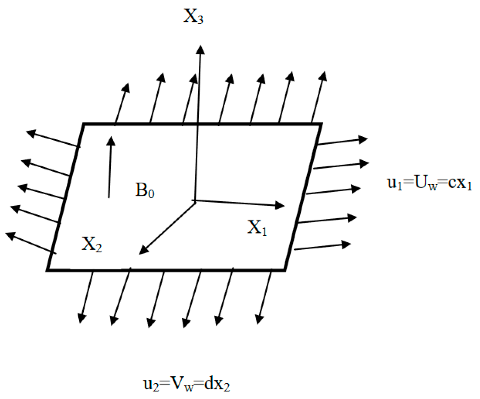
2. Physical Model and Mathematical Formulation

2.1. Rheological Model

Consider the non-Newtonian fluid with time-independent and following the Sisko rheological model; for such types of fluids, the Cauchy’s stress tensor is defined as

$$T=-pI+S$$

(1)

where $S$ is called the extra stress tensor as

$$S=\left[a_1+b_1{\left|\sqrt{\frac{1}{2}tr(A_1^2})\right|}^{n-1}\right]A_1.$$

(2)

in which, for $n>0$ for various fluids, it is considered that $a_1$ & $b_1$ are the physical constants difference, $A_1=\left(gradV\right)+{\left(gradV\right)}^T$, V represents for the vector as velocity, T stands for transposition, and means the first Rivlin-Erickson tensor.

2.2. Governing Equations and Boundary Conditions

The constant, incompressible, conducting, three-dimensional fluid flow, which adheres in the Sisko model, adopts space $x_3>0$. Fluid is moved through an elastic flat sheet in the plane $x_3=0$, with a constant temperature, is continuously stretched in the $x_1$- and $x_2$- directions with linear velocities $c_1{x}_1$ and $d_1{x}_2$, respectively, as shown in Figure 1 (physical model). A uniform magnetic field of strength $B_0$ is applied along $x_3$-direction. It is assumed that the applied electric field, induced magnetic field, and pressure gradient along the stretching sheet are neglected. The uniform ambient temperature is at a distance far away from the sheet and is considered as $T_{\infty }$.

Under the boundary layer approximation, the governing equations for continuity, momentum, and energy are as follows:

$$\frac{\partial u_1}{\partial x_1}+\frac{\partial u_2}{\partial x_2}+\frac{\partial u_3}{\partial x_3}=0,$$

(3)

$$\rho \left(u_1\frac{\partial u_1}{\partial x_1}+u_2\frac{\partial u_1}{\partial x_2}+u_3\frac{\partial u_1}{\partial x_3}\right)=a_1\frac{{\partial }^2{u}_1}{\partial x_3{}^2}-b_1\frac{\partial }{\partial x_3}{\left(-\frac{\partial u_1}{\partial x_3}\right)}^n-\frac{\sigma B_0^2}{\rho }{u}_1,$$

(4)

$$\rho \left(u_1\frac{\partial u_2}{\partial x_1}+u_2\frac{\partial u_2}{\partial x_2}+u_3\frac{\partial u_2}{\partial x_3}\right)=a_1\frac{{\partial }^2{u}_2}{\partial x_3{}^2}-b_1\frac{\partial }{\partial x_3}{\left(-\frac{\partial u_1}{\partial x_3}\right)}^{n-1}\frac{\partial u_2}{\partial x_3}-\frac{\sigma B_0^2}{\rho }{u}_2,$$

(5)

$$u_1\frac{\partial T}{\partial x_1}+u_2\frac{\partial T}{\partial x_2}+u_3\frac{\partial T}{\partial x_3}=\frac{k}{\left(\rho c_p\right)}\frac{{\partial }^{2}T}{\partial x_3{}^2}.$$

(6)

The boundary conditions are as follows:

$$\begin{array}{l}{u}_1=U_w(x_1)=c{x}_1, u_2=V_w\left(x_2\right)=d{x}_2, u_3=0,\\ Case1: \frac{\partial T}{\partial x_3}=-\frac{q_w}{k} (CHF), Case 2: \frac{\partial T}{\partial x_3}=-h_{s}T (NH),\end{array}\} \mathrm{at} x_3=0,$$

(7)

$$u_1\to 0,u_2\to 0,T\to T_{\infty }, \mathrm{as} x_3\to \infty .$$

(8)

2.3. Transformed Problem

By implementing the following transformation variables, the governing coupled partial differential Equations (3)–(6) are converted to coupled ordinary differential equations as below:

$$\begin{array}{l}{u}_1=c_1{x}_1{f}^{\prime }\left({\eta }_1\right), u_2=d_1{x}_2{g}^{\prime }\left({\eta }_1\right),\\ u_3=-c_1{\left(\frac{c_1{}^{n-2}}{\rho /b_1}\right)}^{1/(n+1)}\left[\frac{2n}{n+1}f\left({\eta }_1\right)+\frac{1-n}{1+n}{\eta }_1{f}^{\prime }\left({\eta }_1\right)+g\left({\eta }_1\right)\right]x_1{}^{\raisebox{1ex}{$n-1$}\!\left/ \!\raisebox{-1ex}{$n+1$}\right.},\\ \theta \left({\eta }_1\right)=\frac{k{\mathrm{Re}}_b^{n+1}{x}_1{}^{n/1-n}}{\rho }\left(T-T_{\infty }\right)(CHF), \theta \left({\eta }_1\right)=\frac{T-T_{\infty }}{T_{\infty }}(NH),\\ {\eta }_1=x_3{\left(\frac{c_1{}^{2-n}}{b_1/\rho }\right)}^{1/(n+1)}{x}_1{}^{\raisebox{1ex}{$1-n$}\!\left/ \!\raisebox{-1ex}{$1+n$}\right.}.\end{array}$$

(9)

The equations of momentum and heat transfer can be reduced as

$$\begin{array}{l}A{f}^{‴}\left({\eta }_1\right)+n{\left(f^{″}\left({\eta }_1\right)\right)}^{n-1}{f}^{‴}\left({\eta }_1\right)+\frac{2n}{n+1}f\left({\eta }_1\right)f^{″}\left({\eta }_1\right)-{\left(f^{\prime }\left({\eta }_1\right)\right)}^2\\ +g\left({\eta }_1\right)f^{″}\left({\eta }_1\right)-M{f}^{\prime }\left({\eta }_1\right)=0,\end{array}$$

(10)

$$\begin{array}{l}A{g}^{‴}({\eta }_1)+{\left(-f^{‴}({\eta }_1)\right)}^{n-1}{g}^{‴}({\eta }_1)-\left(n-1\right)g^{″}({\eta }_1)f^{‴}({\eta }_1){\left(-f^{″}({\eta }_1)\right)}^{n-2}\\ +\frac{2n}{n+1}f({\eta }_1)g^{″}({\eta }_1)-{\left(g^{\prime }({\eta }_1)\right)}^2+g({\eta }_1)g^{″}({\eta }_1)-M{g}^{\prime }({\eta }_1)=0,\end{array}$$

(11)

$${\theta }^{″}\left({\eta }_1\right)+\mathrm{Pr}\left(\frac{2n}{n+1}\right)f\left({\eta }_1\right){\theta }^{\prime }\left({\eta }_1\right)+\mathrm{Pr}g\left({\eta }_1\right){\theta }^{\prime }\left({\eta }_1\right)=0,$$

(12)

The boundary conditions are reduced as

$$\begin{array}{l}f\left({\eta }_1\right)=0, g\left({\eta }_1\right)=0, f^{\prime }\left({\eta }_1\right)=1, g^{\prime }\left({\eta }_1\right)=d/c=\alpha ,\\ Case 1 : {\theta }^{\prime }\left({\eta }_1\right)=-1 (CHF), Case 2: {\theta }^{\prime }\left({\eta }_1\right)=-\gamma (1+\theta ({\eta }_1)) (NH),\end{array}\} \mathrm{at} {\eta }_1=0,$$

(13)

$$f^{\prime }({\eta }_1)\to 0,g^{\prime }({\eta }_1)\to 0,\theta \left({\eta }_1\right)\to 0, \mathrm{as} {\eta }_1\to \infty .$$

(14)

where $\alpha =\frac{d}{c}$ is the stretching ratio parameter, prime denotes differentiation with respect to.

We consider the range $0\le \alpha \le 1$, since for $\alpha >1$, the $x_1$- and $x_2$-axes are interchanged [42].

$$\begin{array}{l}{\mathrm{Re}}_a=\frac{\rho x_{1}U}{a}, {\mathrm{Re}}_b=\frac{\rho x_1{}^n{U}^{2-n}}{b}, M=\frac{\sigma B_0^2}{\rho c},\\ A=\frac{{\mathrm{Re}}_b{}^{2/(n+1)}}{{\mathrm{Re}}_a}, \mathrm{Pr}=\frac{x_{1}U{R}_b{}^{-2/(n+1)}}{k/\rho c_p}, \gamma =-\frac{h_s}{{\mathrm{Re}}_b^{n+1}{x}_1{}^{n/(1-n)}}.\end{array}$$

(15)

Note that when $\alpha =1$, the rate of stretching is equal in both $x_1$- as well as $x_2$-directions, which is the axisymmetric-type flow. The unidirectional case is acquired at limit $\alpha \to 0$ and the motion of the fluid is simply in the $x_1{x}_3$-plane, i.e., in Equation (9) both $g$ and $\frac{\partial g}{\partial {\eta }_1}$ become zero.

2.4. Physical Quantities of Engineering Interest

2.4.1. The Coefficients of Skin Friction

One of the leading boundary layer characteristics is the skin-friction coefficient; at $x_3=0$ (near wall), the Shear pressure is dimensionless.

Therefore, the dimensionless coefficients of skin friction in the direction of $x_1$- and $x_2$- respectively, are specified by [36,43]:

$$C_{f{x}_1}=\frac{{\tau }_{x_1{x}_3}}{\raisebox{1ex}{$1$}\!\left/ \!\raisebox{-1ex}{$2$}\right.\rho U_w^2},\hspace{1em}{C}_{f{x}_2}=\frac{{\tau }_{x_2{x}_3}}{\raisebox{1ex}{$1$}\!\left/ \!\raisebox{-1ex}{$2$}\right.\rho U_w^2}.$$

(16)

where ${\tau }_{x_1{x}_3}$ is shear stress in the $x_1$-direction and ${\tau }_{x_2{x}_3}$ is shear stress in $x_2$-direction. These quantities can be described as follows, which are in the dimensionless form:

$$\frac{1}{2}{\mathrm{Re}}_b^{\raisebox{1ex}{$1$}\!\left/ \!\raisebox{-1ex}{$n+1$}\right.}{c}_{f{x}_1}={\left(A{f}^{″}\left({\eta }_1\right)-{\left[-f^{″}\left({\eta }_1\right)\right]}^n\right)}_{{\eta }_1=0},$$

(17)

$$\frac{1}{2}{\mathrm{Re}}_b^{\raisebox{1ex}{$1$}\!\left/ \!\raisebox{-1ex}{$n+1$}\right.}{C}_{f{x}_2}=\frac{V_w}{U_w}{\left[A{g}^{″}\left({\eta }_1\right)+{\left[-f^{″}\left({\eta }_1\right)\right]}^{n-1}{g}^{″}\left({\eta }_1\right)\right]}_{{\eta }_1=0}.$$

(18)

2.4.2. The Local Nusselt Number

The local Nusselt number is symbolized as $N{u}_{x_1}$, which gives the heat transfer rate on the wall defined as [13]:

$$N{u}_{x_1}={\frac{x_1{q}_w}{k\left(T_w-T_{\infty }\right)}|}_{x_3=0}.$$

(19)

where $q_w={-k\left(\frac{\partial T}{\partial x_3}\right)|}_{x_3=0}$ is defined as the wall heat flux, and

$${\mathrm{Re}}_b^{\raisebox{1ex}{$-1$}\!\left/ \!\raisebox{-1ex}{$n+1$}\right.}N{u}_{x_1}=-{\theta }^{\prime }\left(0\right)(CHF) and {\mathrm{Re}}_b^{\raisebox{1ex}{$-1$}\!\left/ \!\raisebox{-1ex}{$n+1$}\right.}N{u}_{x_1}=-{\theta }^{\prime }\left(0\right)(NH).$$

(20)

3. Solution of the Problem

To describe this section succinctly, to solve the Equations (10)–(14), the spectral relaxation method (SRM) is used, this method can be observed in the investigation of Motsa and Makukula [44]. SRM was suggested to address problems of the boundary layer similarity of profiles deteriorating significantly. In this case, the algorithm of SRM for the subject of boundary layer problems having a self-similar condition is described below briefly:

• By implementing the transformation $\frac{\partial f}{\partial {\eta }_1}=p\left({\eta }_1\right)$, the momentum equation order for $f\left({\eta }_1\right)$ is reduced and depicts how the actual equation for $p\left({\eta }_1\right)$ is displayed.
• Assume that $f\left({\eta }_1\right)$ is perceived here from an earlier iteration (directed by $f_r$), in order to build a scheme of iteration for $p\left({\eta }_1\right)$ in which, at the current iteration stage, assume that only linear terms in $p\left({\eta }_1\right)$ are to be estimated (directed by $p_{r+1}$) and for all other remaining terms that are of use, linear and nonlinear are assumed to be familiar from previous iterations. Furthermore, at the preceding iteration, nonlinear terms in $p$ are assessed.
• By implementing the transformation $\frac{\partial g}{\partial {\eta }_1}=q({\eta }_1)$, the momentum equation order for $g({\eta }_1)$ is reduced and depicts how the actual equation for $q({\eta }_1)$ is displayed.
• Assume that $g({\eta }_1)$ is perceived here from an earlier iteration (referred to by $g_r$), in order to build a scheme of iteration for $q({\eta }_1)$ in which, at the current iteration stage, assume that only linear terms in $q({\eta }_1)$ are to be estimated (referred by $q_{r+1}$) and for all other remaining terms that are of use, linear and nonlinear are assumed to be familiar from previous iterations. Furthermore, at the preceding iteration, nonlinear terms in $q$ are assessed.
• In a similar manner to find the remaining governing dependent variables, the iteration schemes are developed and now the variable solutions chosen in the earlier equation are used in the updated solutions.

The concept of decoupling equations with the Gauss–Seidel idea is similar to the above-mentioned technique. This procedure leads to variable coefficients with a sequence of linear differential equations; here, by using traditional mathematical and numerical techniques, linear differential equations are easily solved. In the present analysis, to discretise the differential equations, we have used Chebyshev spectral collocation methods (see, for example, [45,46]). By numerical technique, we determine that ${\left({\eta }_1\right)}_{\infty }=20$, with $\overline{N}=100$ grid points giving a spectral relaxation method with sufficient accuracy.

Because of their solution of a variable coefficient of linear differential equations, spectral approaches are chosen in simple areas with smoothing solutions and a fast execution in terms of discernment, including remarkably high precision. By the above discussed SRM iterative system, Equations (10)–(14) be converted into

$${f^{\prime }}_{r+1}=p_{r+1}, f_{r+1}(0)=0, {g^{\prime }}_{r+1}=q_{r+1}, g_{r+1}(0)=0,$$

(21)

$$\left(A+n{(-{p^{\prime }}_r)}^{n-1}\right){p^{″}}_{r+1}+\left(\frac{2n}{n+1}{f}_r+g_r\right){p^{\prime }}_{r+1}-\left(M\right)p_{r+1}=p_{r+1}^2,$$

(22)

$$\left(A+{(-{p^{\prime }}_r)}^{n-1}\right){p^{″}}_{r+1}+\left(\frac{2n}{n+1}{f}_r+g_r-(n-1){p^{″}}_r{(-{p^{\prime }}_r)}^{n-1}\right){q^{\prime }}_{r+1}-\left(M\right)q_{r+1}=q_{r+1}^2,$$

(23)

$${{\theta }^{″}}_{r+1}+\mathrm{Pr}\left(\frac{2n}{n+1}{f}_r+g_r\right){{\theta }^{\prime }}_{r+1}=0,$$

(24)

For the above iteration scheme, the suitable boundary conditions are considered, which are alluded to as follows:

$$p_{r+1}(0)=1, q_{r+1}(0)=\alpha , {{\theta }^{\prime }}_{r+1}(0)=-1 (CHF), {{\theta }^{\prime }}_{r+1}(0)=-\gamma \left(1+{\theta }_{r+1}(0)\right) (NH),$$

(25)

$$p_{r+1}(\infty )=0, q_{r+1}(\infty )=0, {\theta }_{r+1}(\infty )=0,$$

(26)

where the prime denotes differentiation with respect to ${\eta }_1$. The Chebyshev spectral collocation method is used while solving the decoupled Equations (21)–(24). By using the spectral procedure, the mathematical domain with the interval [0, L] is converted into [−1, 1] using ${\eta }_1=L(\xi +1)/2$, which is the application of the spectral process. At infinity, L is considered for implementing boundary conditions. The implementation of a matrix differentiation $𝒟$ used to estimate derivatives of unknown variables at the collocation points is one of the key ideas of the spectral collocation method as the product of the vector matrix of the form.

$$\frac{\partial f_{r+1}}{\partial {\eta }_1}={\displaystyle \sum _{k=0}^{\overline{N}}{D}_{lk}{f}_r({({\eta }_1)}_k)}=D{f}_r,l=0,1,2,\dots \dots \dots \overline{N}.$$

(27)

where the number of collocation points denoted by $\overline{N}+1$ (grid points) and at the collocation points D = 2.$𝒟$/L, $f={\left[f({\xi }_0),f({\xi }_1),f({\xi }_2),\dots \dots \dots f({\xi }_{\overline{N}})\right]}^T$ is the vector function. Powers of D denote the order of derivatives in higher order.

$$f_r{}^{(p)}=D^p{f}_r,$$

(28)

where the order of the derivative is taken as $p$. For Equations (21)–(24) the spectral method applied, we obtain:

$$A_1{f}_{r+1}=B_1, f_{r+1}({\eta }_1{}_{\overline{N}})=0,$$

(29)

$$A_2{p}_{r+1}=B_2, p_{r+1}({\eta }_1{}_{\overline{N}})=1, p_{r+1}({\eta }_1{}_0)=0,$$

(30)

$$A_3{g}_{r+1}=B_3, g_{r+1}({\eta }_1{}_{\overline{N}})=0 ,$$

(31)

$$A_4{q}_{r+1}=B_4, q_{r+1}({\eta }_1{}_{\overline{N}})=\alpha , q_{r+1}({\eta }_1{}_0)=0,$$

(32)

$$\begin{array}{l}{A}_5{\theta }_{r+1}=B_5, {\displaystyle \sum _{k=0}^{\overline{N}}{D}_{\overline{N}k}}{\theta }_{r+1}({\eta }_1{}_k)=-1(CHF),\\ {\displaystyle \sum _{k=0}^{\overline{N}}{D}_{\overline{N}k}}{\theta }_{r+1}({\eta }_1{}_k)+\gamma {\theta }_{r+1}({\eta }_1{}_k)=-\gamma (NH), {\theta }_{r+1}({\eta }_1{}_0)=0,\end{array}$$

(33)

where

$$A_1=D,B_1=p_{r+1},$$

(34)

$$A_2=\left(A+n{(-{p^{\prime }}_r)}^{n-1}+\right)D^2+\left(\frac{2n}{n+1}{f}_r+g_r\right)D-\left(M\right)I,B_2=p_{r+1}^2,$$

(35)

$$A_3=D,B_3=q_{r+1},$$

(36)

$$A_4=\left(A+{(-{p^{\prime }}_r)}^{n-1}\right)D^2+\left(\frac{2n}{n+1}{f}_r+g_r-(n-1){p^{″}}_r{(-{p^{\prime }}_r)}^{n-1}\right)D-\left(M\right)I,B_4=q_{r+1}^2,$$

(37)

$$A_5=D^2+Pr\left(\frac{2n}{n+1}{f}_r+g_r\right)D,B_5=0$$

(38)

.

In Equations (29)–(33) there is a diagonal matrix, diag [ ], and I is an identity matrix; these are all of size $(\overline{N}+1)\times (\overline{N}+1)$, as the number of grid points $\overline{N}$ is considered, $f,p,g,q$ and $\theta$ are the function values respectively, and subscript $r$ represents the iteration number while evaluating at grid points.

Initial estimates of Equations (25) and (26) to enable the SRM scheme are selected as

$$\begin{array}{l}{f}_0(\eta )=1-e^{-{\eta }_1}, p_0\left(\eta \right)=e^{-{\eta }_1}, g_0(\eta )=\alpha -\alpha e^{-{\eta }_1},\\ q_0\left(\eta \right)=\alpha e^{-{\eta }_1}, {\theta }_0\left(\eta \right)=e^{-{\eta }_1}(CHF), {\theta }_0\left(\eta \right)=\frac{\gamma }{1-\gamma }{e}^{-{\eta }_1}(NH).\end{array}$$

(39)

These are the functions chosen randomly that the boundary conditions satisfy accordingly. The process of iteration is continued until it reaches convergence. At the infinity point, the convergence of the SRM is established as

$$Er=Max\left(\Vert f_{r+1}-f_r\Vert ,\Vert p_{r+1}-p_r\Vert ,\Vert g_{r+1}-g_r\Vert ,\Vert q_{r+1}-q_r\Vert ,\Vert {\theta }_{r+1}-{\theta }_r\Vert \right).$$

(40)

If $\overline{N}$ increased, the scheme accuracy is established until achieving a point where the consistent solutions and the value of the solutions are not changed due to further increment.

Applying the successive over-relaxation (SOR) method to Equations (29)–(33) will considerably strengthen the convergence rate of the SRM algorithm. $\omega$ is included as a parameter for convergence control relaxation under the SOR framework, and the SRM scheme X was invented to obtain:

$$A{X}_{r+1}=(1-\omega )A{X}_r+\omega B.$$

(41)

To improve the accuracy as well as efficiency of the spectral relaxation method, here we applied the SOR method. This shows the results in the next section for $\omega$ < 1.

4. Accelerating the Convergence of the SRM

To solve the required linear matrix equations system as in many other iterative schemes, the SRM scheme defined in the matrix Equations (29)–(33) can be accelerated and enhanced to improve their accuracy. In the study of linear algebra, SOR is consistently used to overcome linear systems such as the Jacobi and Gauss–Seidel approaches in order to speed up the iterative process convergence. Here, we introduce a convergence-controlling relaxation parameter $\omega$ to utilize a similar approach on (35)–(39), summarized as

$$A_1{f}_{r+1}=\left(1-\omega \right)A_1{f}_r+\omega B_1,$$

(42)

$$A_2{p}_{r+1}=\left(1-\omega \right)A_2{p}_r+\omega B_2,$$

(43)

$$A_3{g}_{r+1}=\left(1-\omega \right)A_3{g}_r+\omega B_3,$$

(44)

$$A_4{q}_{r+1}=\left(1-\omega \right)A_4{q}_r+\omega B_4,$$

(45)

$$A_5{\theta }_{r+1}=\left(1-\omega \right)A_5{\theta }_r+\omega B_5.$$

(46)

These are subject to the same boundary conditions as in (29)–(33). This gives the best convergence, depends on the input parameters $\alpha , n, \lambda$ and Pr including magnitude, by the optimal and best choice of the accelerating convergence relaxation parameter $\omega$. In some various cases, the value of $\omega$ accelerated the convergence in the $0.8<\omega <1$ range for some values of $\alpha , n, \lambda$ and Pr, which was observed through numerical experimentation. In the remaining case, it was observed that the relaxation parameter introduction was not useful. It should be notably indicated that $\omega =1$ gives the basic SRM, $\omega <1$ is considered as under relaxation, and $\omega >1$ is considered as over-relaxation.

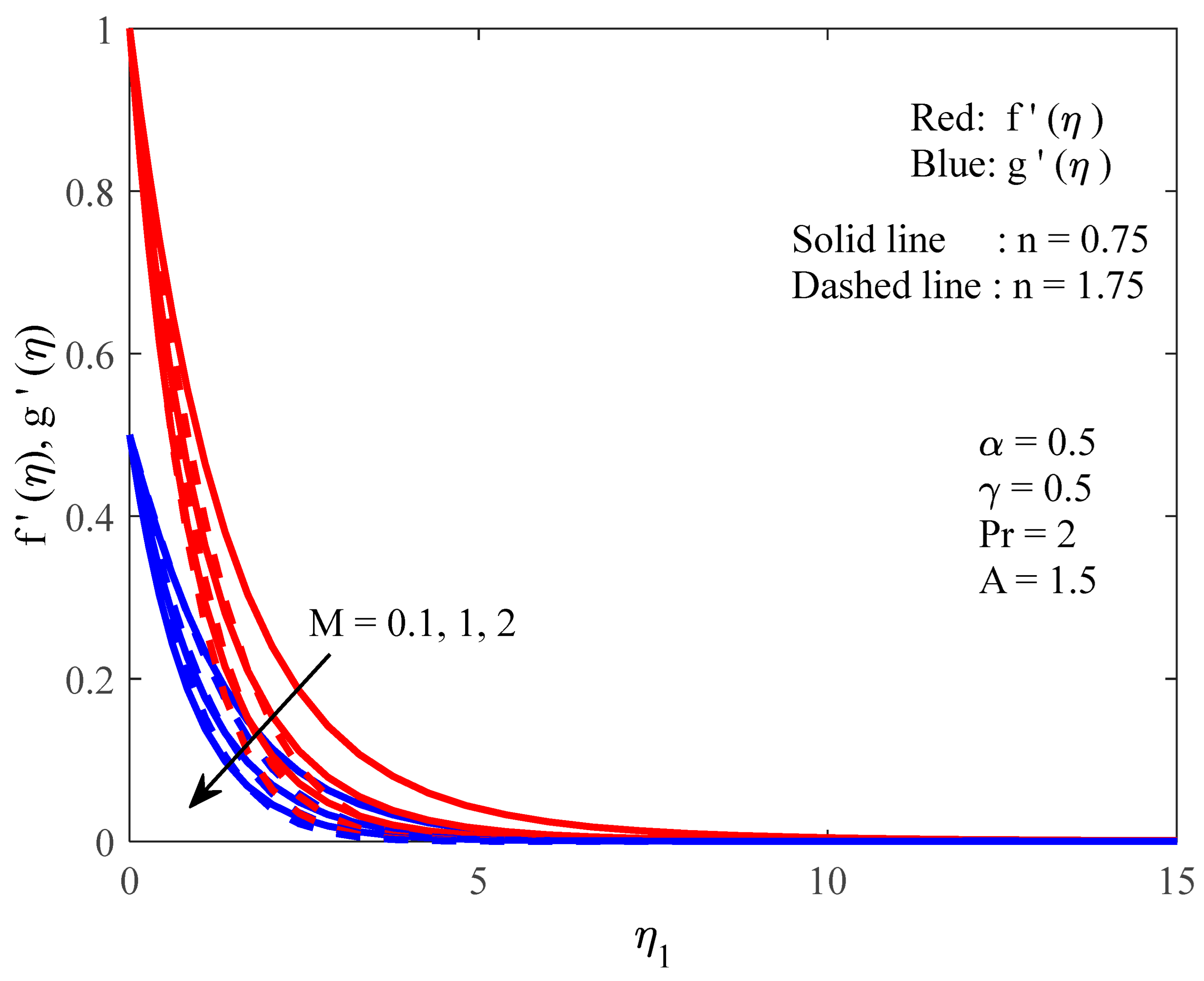
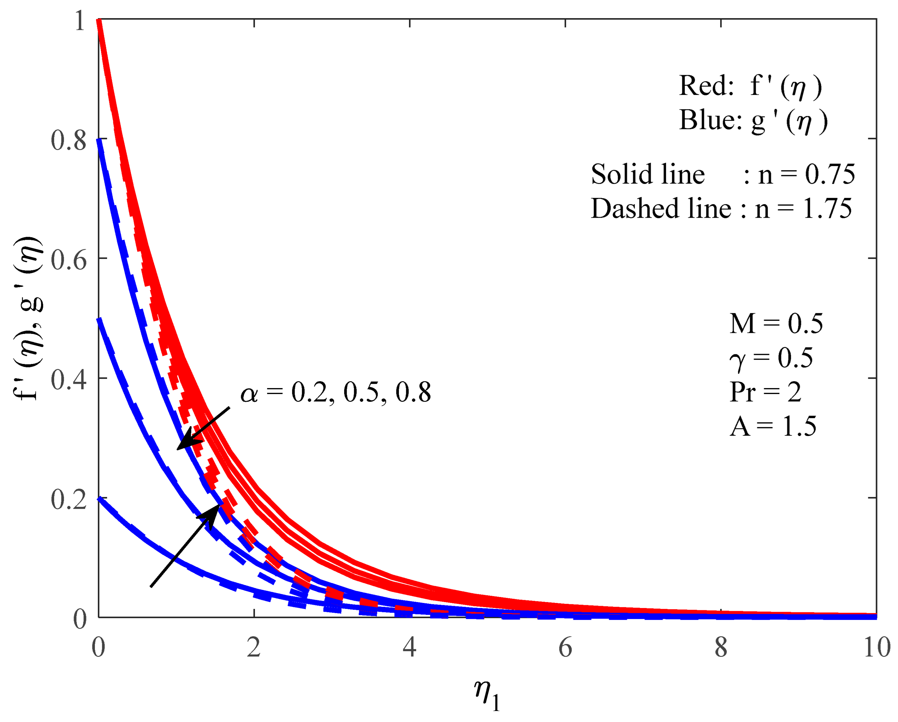
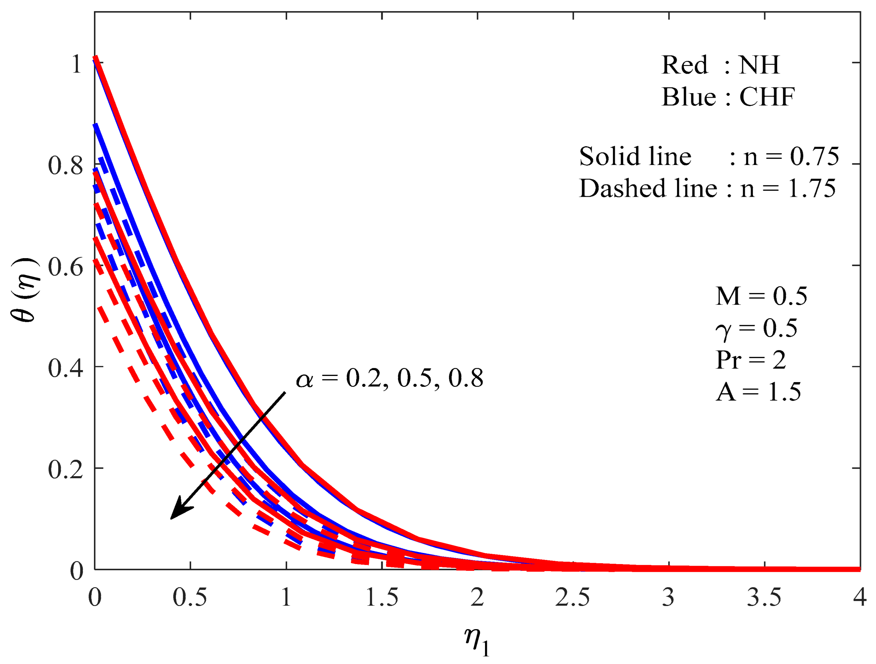
5. Results and Discussion

In this section, our foremost intention is to obtain the clear awareness of the physical conduct of the axial as well as transverse velocity fields and also to consider these with respect to temperature field profiles for some various interesting parameters, such as power law index parameter $n$, magnetic parameter M, stretching ratio parameter $\alpha$, material parameter for Sisko fluid $A$, Prandtl number Pr, and including another constraint, which is nothing but Newtonian heating parameter γ. We solve the system of coupled nonlinear equations by using the well-known technique of the spectral relaxation method (SRM) along with the successive over-relaxation (SOR) method. As part of this research, first we have shown our values along with those of Munir et al. [43], Ariel [4], and Gorla et al. [47] the results of which are given in detail in

Table 1. Resemblance of skin-friction coefficient $f^{″}(0) \& g^{″}(0)$ with the published values of Munir et al. [43], Ariel [4], and Gorla et al. [47] (M = 0, A = 0, n = 1).

$\mathit{\alpha }$	Iter.	${\mathit{f}}^{″}(0)$				${\mathit{g}}^{″}(0)$
		Present Study	Munir et al. [43]	Ariel [4]	Gorla et al. [47]	Present Study	Munir et al. [43]	Ariel [4]	Gorla et al. [47]
0.25	45	−1.04881108	−1.048818	−1.048813	−1.048813	−0.19456383	−0.194567	−0.194565	−0.194564
5.0	35	−1.09309502	−1.093098	−1.093096	−1.093097	−0.46520485	−0.465207	−0.465206	−0.465205
0.75	40	−1.13448575	−1.134487	−1.134486	−1.134485	−0.79461826	−0.794619	−0.794619	−0.794622
1.0	40	−1.17372074	−1.173721	−1.173721	−1.173720	−1.17372074	−1.173721	−1.173721	−1.173720

. We noticed that there is a good deal of similarity between the two. There is no doubt that these results lead to a new debate and trend in the future.

Figure 2 shows the profiles of axial as well as transverse velocities for various values of magnetic parameter M. In the same case, all these effects were simultaneously demonstrated for both shear thinning (pseudo plastic; $0<n<1$) as well as including shear thickening (dilatant; $1<n<2$) fluids. From this figure, it is certainly obvious that the momentum layer thickness in the boundary and the magnitude of the axial as well as transverse velocities are significantly decreased as the strength of Lorentz force increases, because Lorentz force is a retardation force that pulls down the fluid velocity. It shows that the layer thickness at the boundary prominently influences shear thinning fluids, and that this layer thickness exerts greater influence when compared with shear thickening fluids. The temperature profile with different values of $M$ for both the cases of NH and CHF is shown in Figure 3. The excess energy due to Lorentz force accelerates the friction in the fluid, which enhances the fluid temperature. By this observation, the thickness of this boundary layer is elevated highly for shear thinning fluids when compared with shear thickening fluids.

Figure 4 and Figure 5 represent the effects of stretching ratio parameter $\alpha$ on velocity components $f^{\prime }\left(\eta \right)$, $g^{\prime }\left(\eta \right)$ and temperature distributions with shear thinning (n = 0.75) and shear thicknening (1.75). In Figure 4, it is observed that by increasing the values of $\alpha$, velocity in the axial direction decreases, but the opposite phonenomenon has been noticed in the transverse direction. Figure 5 displays that temperature declines by varying $\alpha$.

Figure 6 shows the impact of Sisko fluid material parameter $A$ on axial and transverse velocities for both shear thickening and thinning characteristics. It shows that the velocities for both directions $x_1$ and $x_2$ increase significantly with every growth in $A$.

Figure 7 has been drawn for the temperature distribution profile for $A$. This figure shows that for the growing values of $A$ for the fluids of both shear thinning as well as thickening, the temperature distribution decreases vividly at the surface. Further, there is a thermal boundary layer thickness that appears to be substantially lowered for shear thickening fluid $(n=1.75)$. In addition, this figure shows a resemblance between the power law profile of fluid $(A=0)$ and another profile $(A\ne 0)$, which is a Sisko fluid. This figure clearly demonstrates that when compared to the Sisko fluid, the power law fluid surface temperature is greater.

Prandtl numbers $Pr=0.71$ (air) and $Pr=2$ (water) are framed in Figure 8 with the various values of Newtonian heating conjugate parameter $\gamma$ with the variation of temperature distribution. In this temperature profile, the fluid’s temperature is clearly shown to fall gradually due to considerable growth of $Pr$. In this observation, the viscosity in the fluid escalates by the enhancement of $Pr$, and fluid becomes thicker. This is in line with the physical fact of the decrement in the heat transmission. The heat transfer rate with limited heat efficiency in Newtonian heating from the boundary region is proportionate to local temperature, which is generally referred to as the convective conjugation flow. In this temperature distribution, nothing takes place across the boundary layer area where there is no Newtonian heating parameter, i.e., $\gamma =0$. Further, in this same graph (Figure 8), the increase in the Newtonian heating parameter has been observed by escalating the thermal boundary layer thickness, and consequently, this suggests that it may enhance greatly the surface temperature of the fluid. In this way, this figure shows that the growth in temperature is faster when the conjugate parameter is improved.

Figure 9 and Figure 10 show the skin-friction coefficients for various values of $M, \alpha , A \mathit{and} n$ in both $x$- as well as $y$- directions correspondingly. In these figures, the skin friction in horizontal and vertical directions becomes significantly higher when the power law index is less than one. From these same graphs, we can discuss the relationship among the coefficients of skin friction with the stretching ratio parameter. This discussion shows that the coefficients of skin friction along the directions of $x$ as well as $y$ are enhanced due to the stretching ratio parameter value increase. Further, the magnitude of the skin-friction coefficients increases when the magnetic field parameter increases because the magnetic field slows down the movement of the fluid and therefore these coefficients increase. The variation in rate of mass transfer for various $M, \alpha \mathit{and} n$ values of NH and CHF conditions are shown in Figure 11 and Figure 12, respectively. Here, from a special observation of these two figures, it can be identified that the heat transfer rate escalates for both conditions by each increase of $\alpha$. These statistics show that heat transfer rates are higher for fluids with shear thickening properties, and thus the heat transfer factor leads higher. In addition, the heat transfer rate hikes with the growth of $M$.

Table 2. Numerical values for ${\mathrm{Re}}_x^{-1/2}N{u}_x$ for NH at the surface of the sheet for various values of $Pr \& \gamma$ with $M=0.5,\alpha =0.5 \& A=0.5$.

Pr	Γ	${\mathbf{Re}}_{\mathit{x}}^{-1/2}\mathit{N}{\mathit{u}}_{\mathit{x}}$ for NH
		n = 0.75
		Iter	CPU Time	Basic SRM	$\mathit{\omega }$	Iter	CPU Time	SRM with SOR
	0.1	12	18.76627	4.77995	0.9	9	12.29875	4.77995
0.71		12	20.46802	6.036175	0.9	9	10.91867	6.036175
1		12	24.63855	9.396499	0.9	9	11.36188	9.396499
2		12	22.21707	11.99444	0.9	9	11.10621	11.99444
3		12	22.47097	14.18906	0.9	9	11.82956	14.18906
4		12	22.68458	16.12413	0.9	9	11.61693	16.12413
5	0.2	12	23.24728	2.389975	0.9	9	13.33771	2.389975
2	0.3	12	21.94909	1.593317	0.9	9	13.95093	1.593317
x	0.4	14	21.53128	1.194987	0.9	9	16.56932	1.194987
	0.5	17	28.74275	0.95599	0.85	10	14.70957	0.95599
				n = 1.75
	0.1	11	17.44803	5.716165	0.9	8	12.54738	5.716165
0.71		11	20.91306	7.272926	0.9	8	11.56558	7.272926
1		11	21.13117	11.38285	0.9	8	12.25918	11.38285
2		11	20.89956	14.51542	0.9	8	11.95635	14.51542
3		11	22.29397	17.1434	0.9	8	13.95373	17.1434
4		11	20.65066	19.45184	0.9	8	12.40026	19.45184
5	0.2	11	24.54107	2.858083	0.9	8	13.56013	2.858083
2	0.3	11	24.52556	1.905388	0.9	8	12.39242	1.905388
	0.4	12	23.28151	1.42904	0.9	9	14.90034	1.42904
	0.5	13	23.59943	1.143232	0.9	10	15.30949	1.143232

provides a juxtaposition of the number of iterations and CPU time of the fundamental SRM and the SOR-accelerated SRM (with $\omega$), each method yielding eight-digit-decimal-accurate results for the NH condition. It is possible to note that the higher heat transfer is labeled for the greater value of $Pr$ and consequently the heat transfer rate is higher. The advantage of introducing $\omega$ in this case is that the number of repetitions needed is significantly reduced to provide precise information. To give an example, the combination of SRM under relaxation with $\omega =0.9$ improves from 12 repetitions to 9 repetitions and the convergence of CPU time is also minimized. For the Newtonian heating case, heat transfer rate is reduced.

6. Conclusions

In this investigation, we have presented the flow and heat transfer in Sisko fluid flow over a bidirectional stretching sheet with constant heat flux and Newtonian heating. The following are major conclusions of the present study:

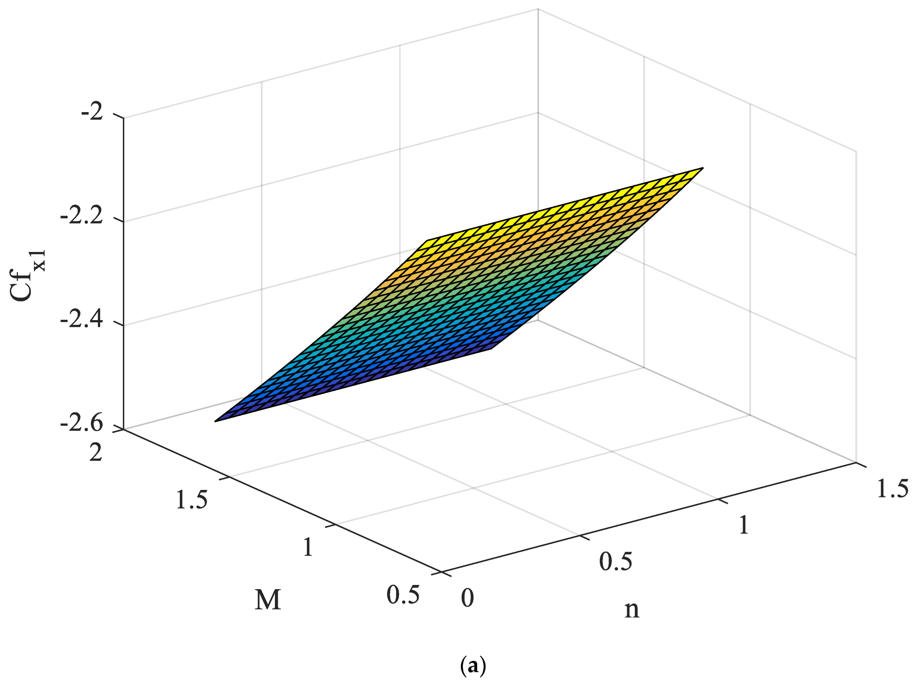
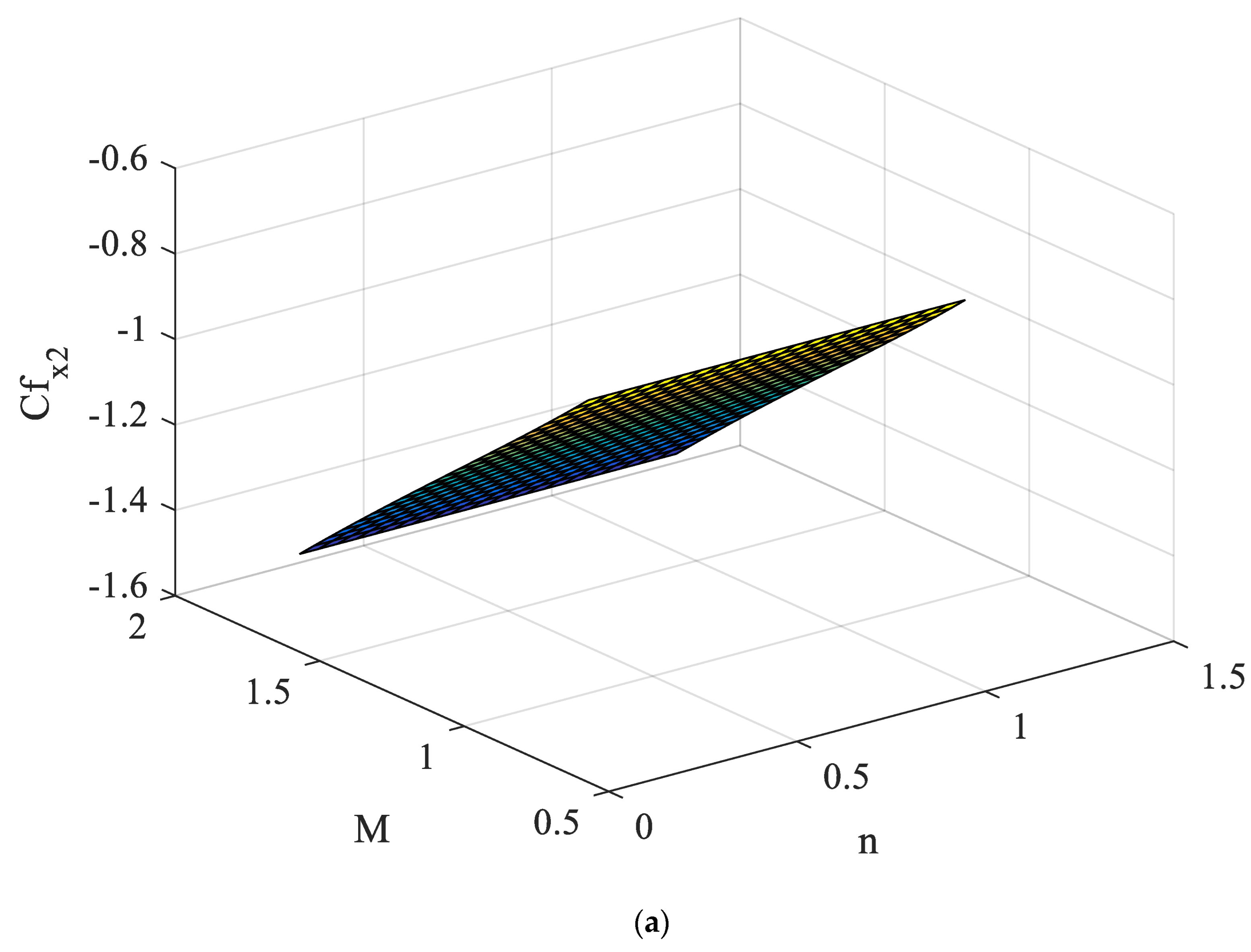
• By increasing the magnetic field strength, the momentum boundary layer thickness decreases, whereas the thermal boundary layer thickness increases.
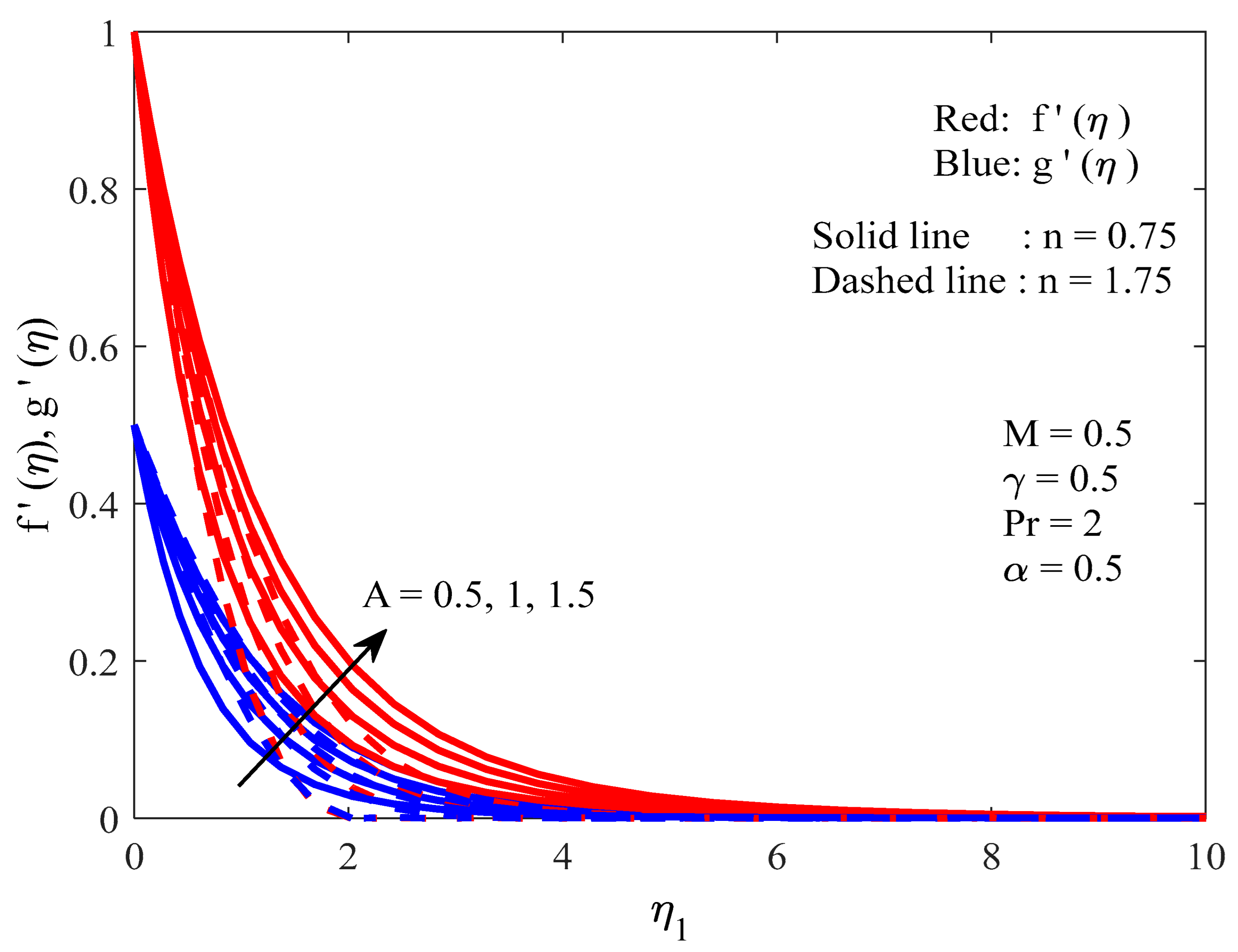
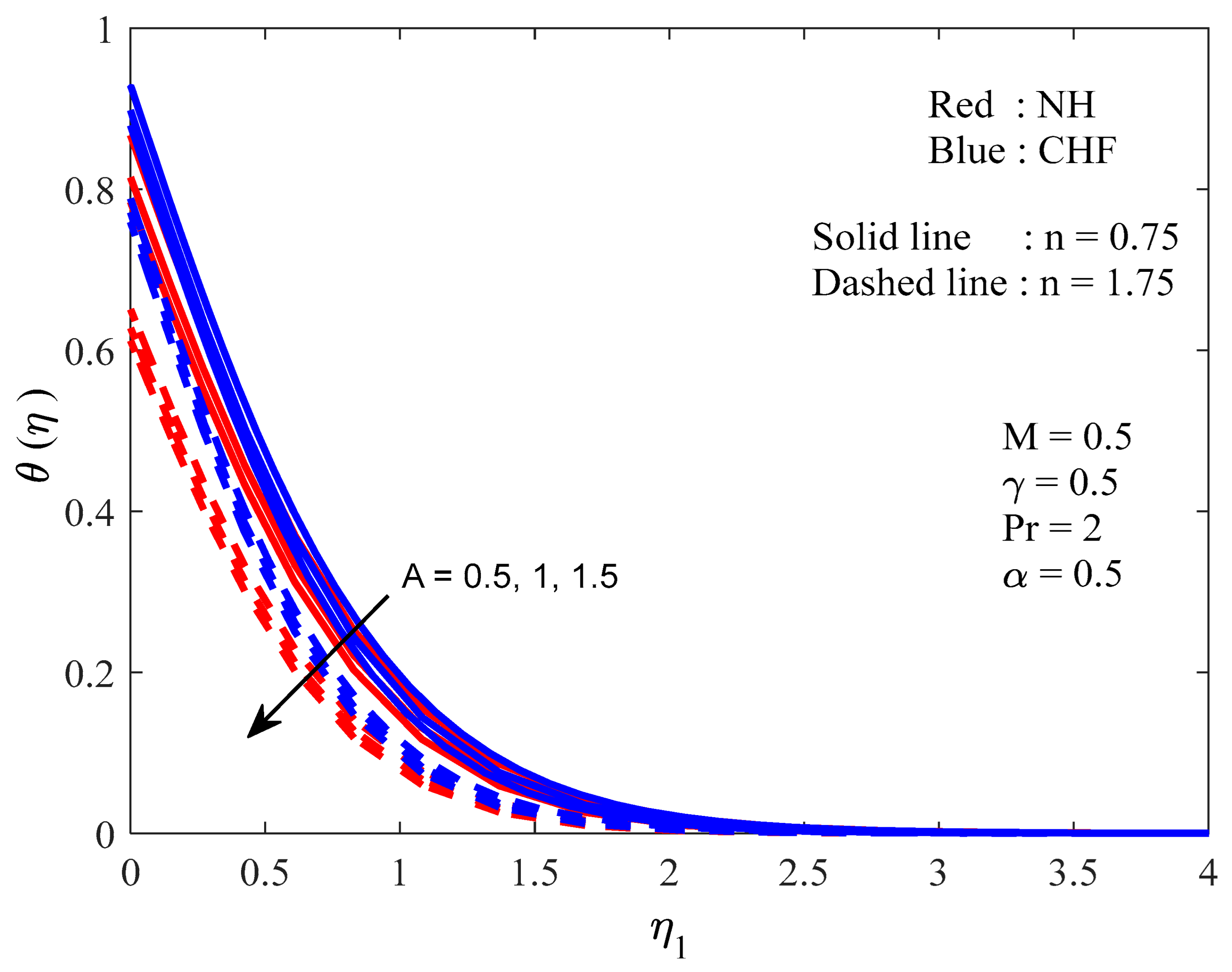
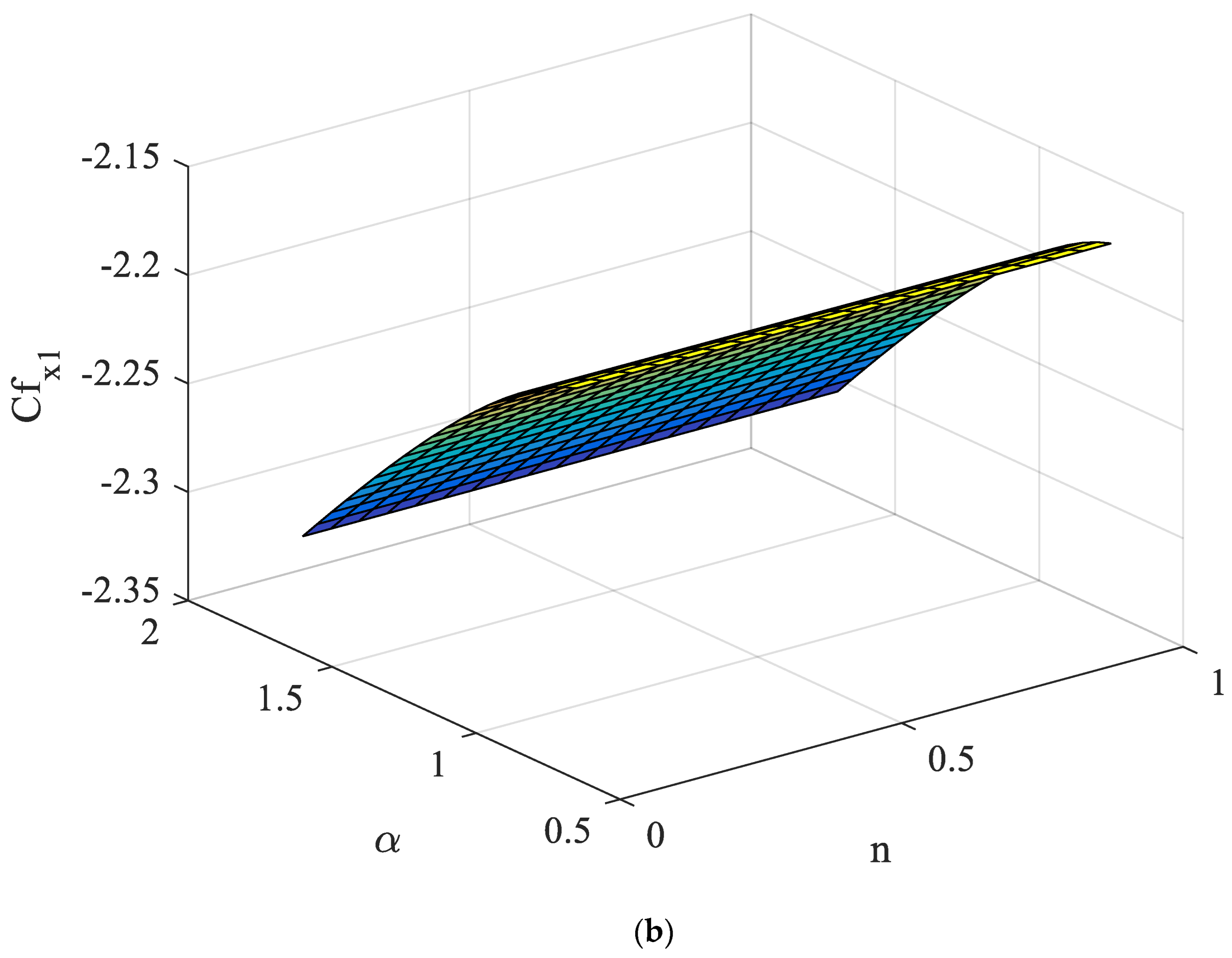
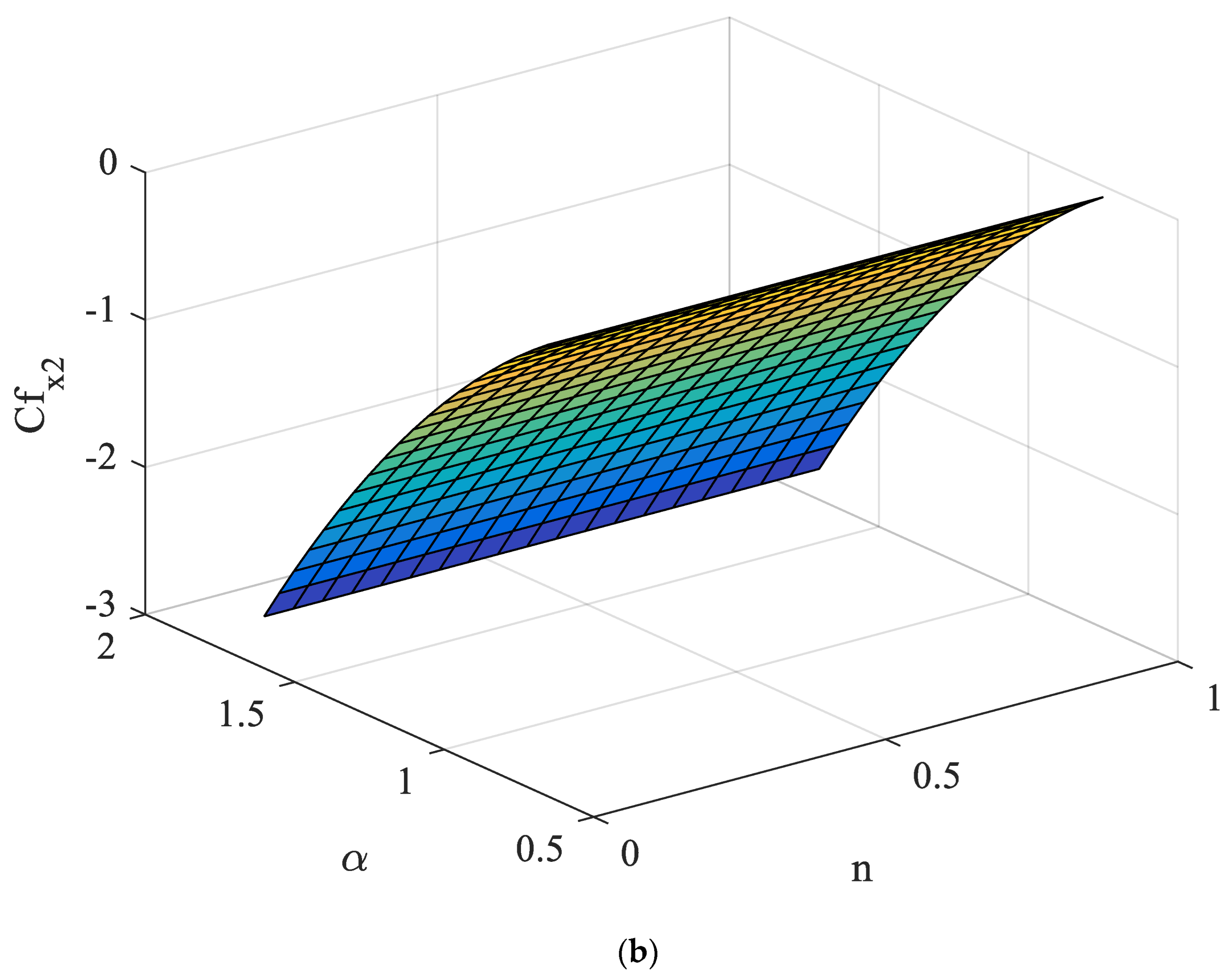
• The velocity distribution in x₁-direction declines, and the opposite phenomenon is observed in x₂-direction, while fluid temperature decreases as the stretching ratio parameter increases.
• With the increase of the Sisko fluid parameter, the velocity in axial and transverse directions increases, whereas the fluid temperature reduces.
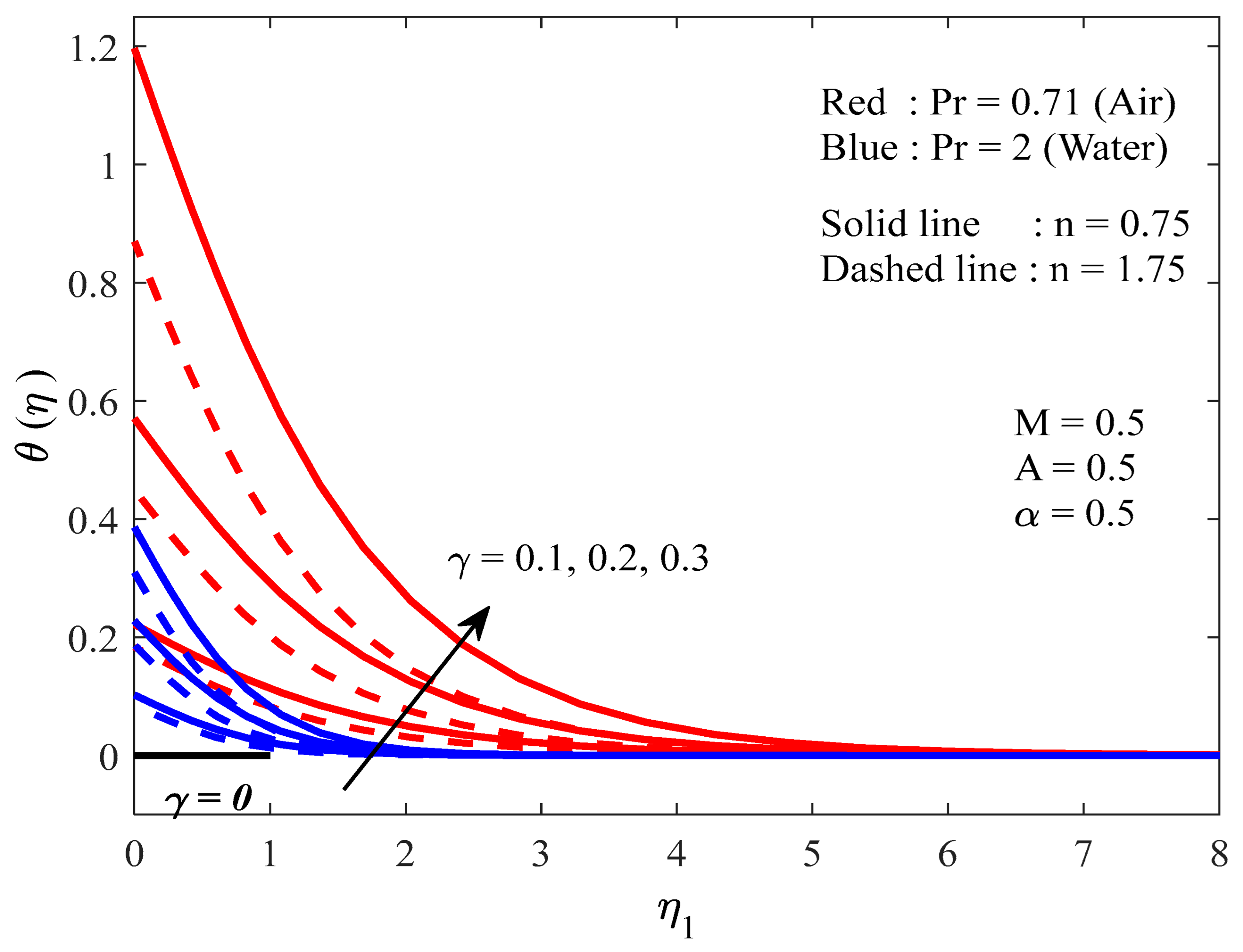
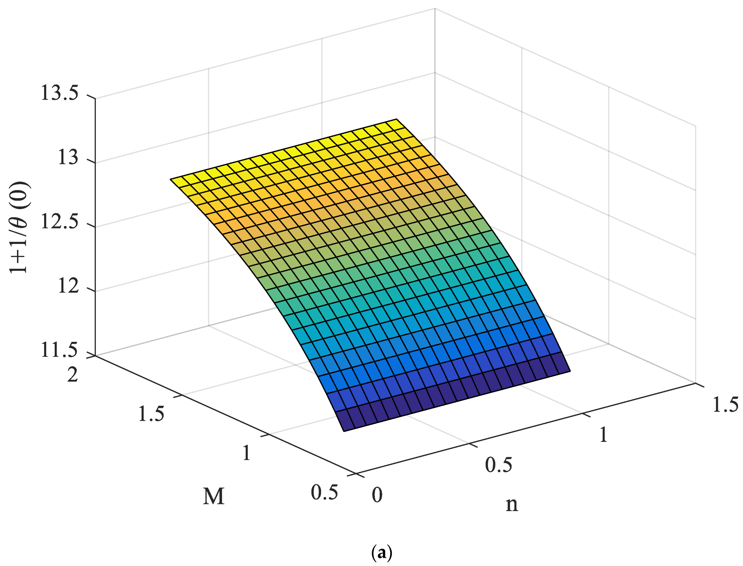
• As the Biot number increases, the fluid temperature increased.
• It was found that successive over (under) relaxation (SOR) techniques would significantly increase the convergence speed of the SRM scheme.
• In this problem, the successful performance of the SRM can be applied in fluid mechanical applications to other various related boundary layer problems.

References

1. Sakiadis, B.C. Boundary Layer Behavior on Continuous Solid Surfaces: 1. Boundary Layer Equations for Two-Dimensional and Axisymmetric Flow. AIChE J. 1961, 7, 26–28. [Google Scholar] [CrossRef]
2. Ishak, A. Thermal boundary layer flow over a stretching sheet in a micropolar fluid with radiation effect. Meccanica 2010, 45, 367–373. [Google Scholar] [CrossRef]
3. Vajravelu, K.; Cannon, J.R. Fluid flow over a nonlinearly stretching sheet. Appl. Math. Comput. 2006, 181, 609–618. [Google Scholar] [CrossRef]
4. Ariel, P.D. Generalized three-dimensional flow due to a stretching sheet. ZAMM-J. Appl. Math. Mech./Z. Angew. Math. Mech. Appl. Math. Mech. 2003, 83, 844–852. [Google Scholar] [CrossRef]
5. Sisko, A.W. The flow of lubricating greases. Ind. Eng. Chem. 1958, 50, 1789–1792. [Google Scholar] [CrossRef]
6. Khan, M.; Shahzad, A. On boundary layer flow of a Sisko fluid over a stretching sheet. Quaest. Math. 2013, 36, 137–151. [Google Scholar] [CrossRef]
7. Megahed, A.M. Flow and heat transfer of non-Newtonian Sisko fluid past a nonlinearly stretching sheet with heat generation and viscous dissipation. J. Braz. Soc. Mech. Sci. Eng. 2018, 40, 492. [Google Scholar] [CrossRef]
8. Upreti, H.; Joshi, N.; Pandey, A.K.; Rawat, S.K. Assessment of convective heat transfer in Sisko fluid flow via stretching surface due to viscous dissipation and suction. Nanosci. Technol. Int. J. 2022, 13, 31–44. [Google Scholar] [CrossRef]
9. Daba, M.; Devaraj, P. Unsteady Boundary Layer Flow of a Nanofluid over a Stretching Sheet with Variable Fluid Properties in the Presence of Thermal Radiation. Phys. Aeromechanics 2016, 23, 403–413. [Google Scholar] [CrossRef]
10. Khan, M.; Malik, R.; Munir, A.; Khan, W.A. Flow and heat transfer to Sisko nanofluid over a nonlinear stretching sheet. PLoS ONE 2015, 10, e0125683. [Google Scholar] [CrossRef]
11. Munir, A.; Shahzad, A.; Khan, M. Forced Convective Heat Transfer in Boundary Layer Flow of Sisko Fluid over a Nonlinear Stretching Sheet. PLoS ONE 2014, 9, e100056. [Google Scholar] [CrossRef] [PubMed]
12. Uddin, M.J.; B’eg, O.A.; Khan, W.A.; Ismail, A.I. Effect of Newtonian Heating and Thermal Radiation on Heat and Mass Transfer of Nanofluids over a Stretching Sheet in Porous Media. Heat Transf. Asian Res. 2014, 44, 681–695. [Google Scholar] [CrossRef]
13. Shen, M.; Wang, F.; Chen, H. MHD Mixed Convection Slip Flow near a Stagnation-Point on a Nonlinearly Vertical Stretching Sheet. Bound. Value Probl. 2015, 2015, 78. [Google Scholar] [CrossRef] [Green Version]
14. Salleh, M.Z.; Nazar, R.; Pop, I. Boundary Layer Flow and Heat Transfer over a Stretching Sheet with Newtonian Heating. J. Taiwan Inst. Chem. Eng. 2010, 41, 651–655. [Google Scholar] [CrossRef]
15. Hussanan, A.; Salleh, M.Z.; Tahar, R.M.; Khan, I. Unsteady Boundary Layer Flow and Heat Transfer of a Casson Fluid past an Oscillating Vertical Plate with Newtonian Heating. PLoS ONE 2014, 9, e108763. [Google Scholar] [CrossRef] [Green Version]
16. Pavlov, K.B. Magnetohydromagnetic Flow of an Incompressible Viscous Fluid Caused by Deformation of a Surface. Magn. Gidrodin. 1974, 4, 146–147. [Google Scholar]
17. Sapunkov, Y.G. Self-Similar Solutions of non-Newtonian Fluid Boundary Layer in MHD. Fluid Dyn. 1967, 2, 77–82. [Google Scholar] [CrossRef]
18. Elghabaty, S.S.; Rahman, G.M.A. Magnetohydrodynamic Boundary-Layer Flow for a non-Newtonian Fluid past a Wedge. Astrophys. Space Sci. 1988, 141, 9–19. [Google Scholar] [CrossRef]
19. Jayachandra Babu, M.; Sandeep, N. MHD non-Newtonian Fluid Flow over a Slandering Stretching Sheet in the presence of Cross-Diffusion Effects. Alex. Eng. J. 2016, 55, 2193–2201. [Google Scholar] [CrossRef] [Green Version]
20. Parida, S.K.; Panda, S.; Rout, B.R. MHD Boundary Layer Slip Flow and Radiative non-linear Heat Transfer over a Flat Plate with Variable Fluid Properties and Thermophoresis. Alex. Eng. J. 2015, 54, 941–953. [Google Scholar] [CrossRef] [Green Version]
21. Prasad, K.V.; Pal, D.; Datti, P.S. MHD Power-Law Fluid Flow and Heat Transfer over a non-Isothermal Stretching Sheet. Commun. Nonlinear Sci. Numer. Simul. 2009, 14, 2178–2189. [Google Scholar] [CrossRef] [Green Version]
22. Datti, P.S.; Prasad, K.V.; Subhas Abel, M.; Joshi, A. MHD Visco-Elastic Fluid Flow over a non-Isothermal Stretching Sheet. Int. J. Eng. Sci. 2004, 42, 935–946. [Google Scholar] [CrossRef]
23. Prasad, K.V.; Pal, D.; Umesh, V.; Prasanna Rao, N.S. The Effect of Variable Viscosity on MHD Viscoelastic Fluid Flow and Heat Transfer over a Stretching Sheet. Commun. Nonlinear Sci. Numer. Simul. 2010, 15, 331–344. [Google Scholar] [CrossRef]
24. Gangadhar, K. Soret and Dufour Effects on Hydro Magnetic Heat and Mass Transfer over a Vertical Plate with a Convective Surface Boundary Condition and Chemical Reaction. J. Appl. Fluid Mech. 2013, 6, 95–105. [Google Scholar]
25. Gangadhar, K. Radiation, Heat Generation and Viscous Dissipation Effects on MHD Boundary Layer Flow for the Blasius and Sakiadis Flows with a Convective Surface Boundary Condition. J. Appl. Fluid Mech. 2015, 8, 559–570. [Google Scholar] [CrossRef]
26. Ma, Y.; Mohebbi, R.; Rashidi, M.M.; Yang, Z.; Sheremet, M. Numerical study of MHD nanofluid natural convection in a baffled U-shaped enclosure. Int. J. Heat Mass Transf. 2019, 130, 123–134. [Google Scholar] [CrossRef]
27. Ma, Y.; Mohebbi, R.; Rashidi, M.M.; Yang, Z. MHD forced convection of MWCNT-Fe2O4/water hybrid nanofluid in a partially heated τ-shaped channel using LBM. J. Therm. Anal. Calorim. 2019, 136, 1723–1735. [Google Scholar] [CrossRef]
28. Ma, Y.; Mohebbi, R.; Rashidi, M.M.; Yang, Z. MHD convective heat transfer of Ag-MgO/water hybrid nanofluid in a channel with active heaters and coolers. Int. J. Heat Mass Transf. 2019, 137, 714–726. [Google Scholar] [CrossRef]
29. Bhatti, M.M.; Mishra, S.R.; Abbas, T.; Rashidi, M.M. A mathematical model of MHD nanofluid flow having gyrotactic microorganisms with thermal radiation and chemical reaction effects. Nat. Comput. Appl. 2018, 30, 1237–1249. [Google Scholar] [CrossRef]
30. Shah, N.A.; Ahmed, N.; Elnaqeeb, T.; Rashidi, M.M. Magnetohydrodynamic free convection flows with thermal memory over a moving vertical plate in porous medium. J. Appl. Comput. Mech. 2019, 5, 150–161. [Google Scholar]
31. Abbas, A.; Noreen, A.; Ali, M.A.; Ashraf, M.; Alzahrani, E.; Marzouki, R.; Goodarzi, M. Solar radiation over a roof in the presence of temperature-dependent thermal conductivity of a Casson flow for energy saving in buildings. Sustain. Energy Technol. Assess. 2022, 53, 102606. [Google Scholar] [CrossRef]
32. Abbas, A.; Jeelani, M.B.; Alharthi, N.H. Magnetohydrodynamic effects on third-grade fluid flow and heat transfer with darcy–forchheimer law over an inclined exponentially stretching sheet embedded in a porous medium. Magnetochemistry 2022, 8, 61. [Google Scholar] [CrossRef]
33. Wu, W.T.; Massoudi, M. Recent advances in mechanics of non-Newtonian fluids. Fluids 2020, 5, 10. [Google Scholar] [CrossRef] [Green Version]
34. Tao, C.; Wu, W.T.; Massoudi, M. Natural convection in a non-Newtonian fluid: Effects of particle concentration. Fluids 2019, 4, 192. [Google Scholar] [CrossRef] [Green Version]
35. Baranovskii, E.S.; Domnich, A.A.; Artemov, M.A. Optimal boundary control of non-isothermal viscous fluid flow. Fluids 2019, 4, 133. [Google Scholar] [CrossRef] [Green Version]
36. Sarkar, S.; Jana, R.N.; Das, S. Activation energy impact on radiated magneto-Sisko nanofluid flow over a stretching and slipping cylinder: Entropy analysis. Multidiscip. Model. Mater. Struct. 2020, 16, 1085–1115. [Google Scholar] [CrossRef]
37. Venkata Subba Rao, M.; Gangadhar, K.; Varma, P.L.N. A spectral relaxation method for three-dimensional MHD flow of nanofluid flow over an exponentially stretching sheet due to convective heating: An application to solar energy. Indian J. Phys. 2018, 92, 1577–1588. [Google Scholar] [CrossRef]
38. Gangadhar, K.; Keziya, K.; Ibrahim, S.M. Effect of thermal radiation on engine oil nanofluid flow over a permeable wedge under convective heating: Keller box method. Multidiscip. Model. Mater. Struct. 2019, 15, 187–205. [Google Scholar]
39. Gangadhar, K.; Kannan, T.; Sakthivel, G.; Dasaradha Ramaiah, K. Unsteady free convective boundary layer flow of a nanofluid past a stretching surface using a spectral relaxation method. Int. J. Ambient. Energy 2020, 41, 609–616. [Google Scholar] [CrossRef]
40. Sobhana Babu, P.R.; Venkata Subba Rao, M.; Gangadhar, K. Boundary layer flow of radioactive non-Newtonian nanofluid embedded in a porous medium over a stretched sheet using the spectral relaxation method. Mater. Today Proc. 2019, 19, 2672–2680. [Google Scholar] [CrossRef]
41. Gangadhar, K.; Narasimharao, N.S.L.V.; Satyanarayana, B. Thermal diffusion and viscous dissipation effects on magnetohydrodynamic heat and mass filled with TiO2 and Al2O3 water based nanofluids. Comput. Therm. Sci. 2019, 11, 523–539. [Google Scholar] [CrossRef]
42. Wang, C.Y. The Three Dimensional Flow due to a Stretching Flat Surface. Phys. Fluids 1984, 27, 1915–1917. [Google Scholar] [CrossRef]
43. Munir, A.; Shahzad, A.; Khan, M. Convective Flow of Sisko Fluid over a Bidirectional Stretching Surface. PLoS ONE 2015, 10, e0130342. [Google Scholar] [CrossRef] [PubMed]
44. Motsa, S.S.; Makukula, Z.G. On spectral relaxation method approach for steady von Karman flow of a Reiner-Rivlin fluid with Joule heating, viscous dissipation and suction/injection. Cent. Eur. J. Phys. 2013, 11, 363–374. [Google Scholar] [CrossRef]
45. Canuto, C.; Hussaini, M.V.; Quarteroni, A.; Zang, T.A. Spectral Methods in Fluid Dynamics; Springer: Berlin, Germany, 1988. [Google Scholar]
46. Trefethen, L.N. Spectral Methods in MATLAB; SIAM: Philadelphia, PA, USA, 2000. [Google Scholar]
47. Gorla, R.S.R.; Pop, I.; Dakappagari, V. Three-Dimensional Flow of a Power-Law Fluid due to a Stretching Flat Surface. ZAMM J. Appl. Math. Mech. 1995, 75, 389–394. [Google Scholar] [CrossRef]
Figure 1. Physical model of the problem.
Energies 16 03183 g001
Figure 2. The bidirectional (axial and transverse) velocity distribution profile with the influence of M .
Energies 16 03183 g002
Figure 3. The temperature distribution profile with the influence of M .
Energies 16 03183 g003
Figure 4. The bidirectional (axial and transverse) velocity distribution profile with the influence of α .
Energies 16 03183 g004
Figure 5. The temperature distribution profile with the influence of α .
Energies 16 03183 g005
Figure 6. The bidirectional (axial and transverse) velocity distribution profiles with the influence of A.
Energies 16 03183 g006
Figure 7. The temperature distribution profiles with the influence of A .
Energies 16 03183 g007
Figure 8. The temperature distribution profile for different values of γ   &   P r .
Energies 16 03183 g008
Figure 9. (a): A 3D plot for C f x 1 -direction for different values of M   &   n . (b): A 3D plot for C f x 1 -direction for different values of α   &   n .
Energies 16 03183 g009aEnergies 16 03183 g009b
Figure 10. (a): Three-dimensional plot for C f x 2 -direction for different values of M   &   n . (b): Three-dimensional plot for C f x 2 -direction for different values of α   &   n .
Energies 16 03183 g010aEnergies 16 03183 g010b
Figure 11. (a): Three-dimensional plot for Nusselt number in NH case for different values of M   &   n . (b): Three-dimensional plot for Nusselt number in NH case for different values of α   &   n .
Energies 16 03183 g011aEnergies 16 03183 g011b
Figure 12. (a): Three-dimensional plot for Local Nusselt number in CHF case for different values of M   &   n . (b): Three-dimensional plot for Nusselt number in CHF case for different values of α   &   n .
Energies 16 03183 g012aEnergies 16 03183 g012b