Comparison of Standalone and Hybrid Machine Learning Models for Prediction of Critical Heat Flux in Vertical Tubes

Abstract

Critical heat flux (CHF) is an essential parameter that plays a significant role in ensuring the safety and economic efficiency of nuclear power facilities. It imposes design and operational restrictions on nuclear power plants due to safety concerns. Therefore, accurate prediction of CHF using a hybrid framework can assist researchers in optimizing system performance, mitigating risk of equipment failure, and enhancing safety measures. Despite the existence of numerous prediction methods, there remains a lack of agreement regarding the underlying mechanism that gives rise to CHF. Hence, developing a precise and reliable CHF model is a crucial and challenging task. In this study, we proposed a hybrid model based on an artificial neural network (ANN) to improve the prediction accuracy of CHF. Our model leverages the available knowledge from a lookup table (LUT) and then employs ANN to further reduce the gap between actual and predicted outcomes. To develop and assess the accuracy of our model, we compiled a dataset of around 5877 data points from various sources in the literature. This dataset encompasses a diverse range of operating parameters for two-phase flow in vertical tubes. The results of this study demonstrate that the proposed hybrid model performs better than standalone machine learning models such as ANN, random forest, support vector machine, and data-driven lookup tables, with a relative root-mean-square error (rRMSE) of only 9.3%. We also evaluated the performance of the proposed hybrid model using holdout and cross-validation techniques, which demonstrated its robustness. Moreover, the proposed approach offers valuable insights into the significance of various input parameters in predicting CHF. Our proposed system can be utilized as a real-time monitoring tool for predicting extreme conditions in nuclear reactors, ensuring their safe and efficient operation.

1. Introduction

The profitability and reliability of heat generating systems, especially nuclear power plants, strongly depend on their safety and regulatory restrictions. Extremely cautious approaches are undertaken to establish such safety and regulatory limits since they are associated with considerable margins to account for design inaccuracies and other possible uncertainties [1]. Departure from nucleate boiling (DNB) is one of the safety limitations encountered when analyzing the safety of two-phase flow boiling systems, including heat exchangers, high-power electronic devices, refrigeration systems, and especially nuclear reactor cores [2]. In a water-cooled reactor, DNB is one of the most significant parameters to the integrity of the reactor core, but is among the least understood in thermal-hydraulic instability [3]. The nucleate boiling heat flux cannot be increased beyond a certain value known as critical heat flux (CHF). The heating system eventually fails as a result of a sharp decrease in the heat-transfer coefficient [4].

In a pressurized water reactor (PWR), overheating occurs when the heating surface temperature suddenly rises and reaches the CHF limit. Therefore, operation of the boiling system must be interrupted and allowed to cool down, resulting in a loss of production. In an extreme scenario, it may lead to a reactor core meltdown [5]. Consequently, an accurate prediction of CHF is essential for the safety of the heat generating system as well as in the nuclear heat transfer process and must be considered when analyzing the safety of power reactors. Furthermore, CHF is a critical safety parameter in nuclear reactor design that should be kept to an acceptable limit [6]. The DNBR (Departure from Nucleate Boiling Ratio) is the minimum CHF ratio that ensures the safe operation of reactors between the expected CHF and actual operational heat flux. The DNBR value varies both axially and radially across the fuel length. In order to maintain safety, the MDNBR (Minimum DNBR) value must be greater than one at all points in the core. Specifically for commercial pressurized water reactors (PWR), the MDNBR value should be at least 1.3 during full power transients to provide an adequate safety margin [7]. This phenomenon is also related to variation in heat transfer coefficient. Hence, predicting CHF is critical for the device’s safety. Extensive experimental and theoretical research has been conducted over the last few decades to explore CHF. Despite extensive research, the exact mechanism responsible for the development of CHF has not been universally agreed upon, making it challenging to establish a reliable means of predicting CHF with certainty [8]. There is no consensus on its trigging mechanism because of the extremely complicated nature of heat transport in boiling [9].

There are several prediction tools available to thermal-hydraulic researchers, ranging from the best-fit empirical correlations, data-driven look-up tables (LUT), to physics-driven analytical models [10]. However, each of these approaches have their own constraints and applicability limits. On the one hand, these best-fit empirical correlations are simple to apply but can only be used in a limited number of situations for specific dimensions and operating requirements. Among the commonly used CHF models in flow boiling include: Biasi correlation [11], Bowring correlation [12], Westinghouse (W-3) correlation [13], Katto correlation [14], Groeneveld 2006 LUT [15], Tong correlation [13], and Electric Power Research Institute (EPRI) correlation [16]. These models are highly dependent upon assumptions, i.e., limited knowledge of the mechanism’s underlying physics, which varies according to the flow regime [17]. Typically, these empirical models are divided into six types, depending on their mechanism: superheat limit bubbly liquid layer mechanism, near-wall bubble crowding and the limit of vapor removal mechanism, dry-off the mechanism’s sublayer of liquid, the process of interfacial lift-off, liquid flow blockage mechanism and separation boundary-layer mechanism [2]. Among these models, the superheat limit bubbly liquid layer mechanism has drawn much interest since it is supported by experimental data. On the other hand, data-driven LUTs demand the use of an estimator to avoid irrelevant irregularities due to data distribution, such as point selection and flattening.

Recent computing advances and optimization methodologies have assisted artificial intelligence (AI)-based techniques to emerge as an alternate strategy to investigate and analyze complex systems using state-of-the-art, data-driven techniques. Artificial neural network (ANN) is among the most popular choices in this area due to its performance for highly nonlinear functions [18]. Numerous variants of ANNs have been developed and implemented in diverse domains, including nuclear power engineering. These ANNs have been used for tasks such as estimating core parameters related to safety, optimizing nuclear fuel management systems, predicting radioactive dose rates in accident scenarios, diagnosing faults, controlling and monitoring nuclear power plants, studying nuclear reactor nonlinear dynamics, and anticipating accidental scenarios. Saleem et al. utilized a feed-forward type deep neural network (DNN) to predict core neutronic parameters of the Ringhals-1 boiling water reactor (BWR) unit [19]. Similarly, Hedayat et al. used cascade feed-forward neural networks to forecast core safety parameters [20] and optimize core configuration design using a hybrid ANN for a research reactor [21]. Zubair et al. employed various machine learning techniques to analyze the safety of a reactor [22], while Faria et al. optimized fuel patterns in nuclear reactors using ANNs [23]. Kim et al. employed an ANN and a fuzzy rule-based system to determine the optimal fuel loading pattern in a nuclear power plant [24]. Desterro et al. utilized a 5-layer deep ANN to predict accidental radioactive releases in nuclear reactors [25], and Yong et al. used deep auto-encoders for real-time anomaly detection in nuclear reactors to enhance safety [26]. Saeed et al. used a DNN for fault diagnosis in nuclear reactors [27], while Guo et al. used a DNN for fault detection in nuclear fuel assemblies [28]. Yiru et al. utilized neural networks for the safety analysis of nuclear power plant control and monitoring systems [29]. Bae et al. employed a two-step ANN to detect the severity and type of faults using an alarm and monitoring system [30], while Adail et al. utilized recurrent neural networks for modeling reactor core dynamics in nuclear power plants (NPPs) [31]. Finally, Koo et al. used a DNN to detect water levels in a reactor core during an accidental scenario [32]. Overall, these studies highlight the versatility of ANNs in nuclear power engineering and their potential to improve safety, optimize reactor performance, and predict critical scenarios. Bildirici and colleagues employed a multi-layer perceptron (MLP)-based neural network approach to investigate the nonlinear relationship between chaotic precious metal and oil prices and volatilities. Their study yielded valuable insights into the nonlinear tail dependence [33]. Furthermore, they integrated the MLP with Markov-switching vector autoregressive analysis to perform regime-dependent sensitivity analysis, which allowed for the assessment of the intricate and nonlinear connections between CO2 emissions, economic development, and petrol prices [34].

In this regard, few researchers used ANN for CHF prediction. Yapo et al. (1992) first used a hybrid Kohonen-BP neural network to predict CHF [35]. In this study, 440 experimental samples were used as reference data to train and test the network [35]. Moon et al. (1996) developed a backpropagation neural network (BPN) for parametric analysis of CHF using three assumptions including fixed inlet, outlet, and local conditions [36]. Mazzola (1997) used two layers BPN to predict water subcooled CHF based on 1888 experimental data points [37]. The effect of heating length on DNB was investigated by Lee et al. (2000) using a BPN [38]. Kim et al. (2000) studied 130 experiment data to detect CHF using spatiotemporal neural network and wavelet transform [39]. Su et al. (2002) used the 1995 look-up table to predict CHF using BPN with three different conditions: inlet, outlet, and local conditions [40]. Su et al. (2003) used BPN to analyze the CHF in circular vertical pipes under low pressure and flow oscillation conditions. Their study was based on 136 experimental data points [41]. Zaferanlouei et al. (2010) used an FNN and HONN to predict CHF near critical pressure using 111 CHF experimental data [42]. In 2011, Cong et al. used dimensionless groups as input parameters using 1079 CHF experimental data from the literature [43]. In this study, the genetic neural network was trained to anticipate CHF on the heating surface with impinging jets in saturated forced convective boiling [43]. Jiang et al. (2013) used SVM to predict critical heat flux for fixed inlet, outlet, and local conditions [44]. But in all these publications, very limited experimental data is used to train and evaluate the model, and none of those employed cross-validation. Random forest is a frequently utilized tree-based ensemble algorithm for regression; however, its application in engineering is somewhat restricted compared to other fields. While random forest has proven to be a powerful tool in data analysis and machine learning applications, its performance in certain engineering contexts can be limited due to various factors such as the complexity and size of the data, as well as the underlying mathematical models and assumptions involved. Despite these limitations, there are still instances where random forest can provide valuable insights and predictive capabilities in engineering applications [45].

It is evident from the above summary that predicting CHF is a complex process that cannot be achieved through a deterministic theory, as it relies on multiple variables. This complication can be addressed by using ANN. The aim of this study is to present a new method for predicting CHF that employs a hybrid framework by combining machine learning algorithms with an LUT. The proposed approach enhances prediction accuracy by utilizing a larger dataset and k-fold cross-validation, thereby improving the generalization capacity of proposed model. Unlike many recent studies that rely solely on standalone ML techniques and limited data, the proposed approach utilizes a more comprehensive dataset and more rigorous testing methodology. This study introduces a novel method that has the potential to significantly improve the accuracy of CHF predictions. Section 2 describes the materials and methods, including the dataset description and study methodology. Section 3 explains the experimental setup and implementation details of standalone models and novel hybrid frameworks developed. Section 4 describes the performance details of standalone models and their comparison with the proposed hybrid framework for the prediction of CHF. In conclusion, Section 5 summarizes the findings of the study and offers recommendations for future research.

2. Materials and Methods

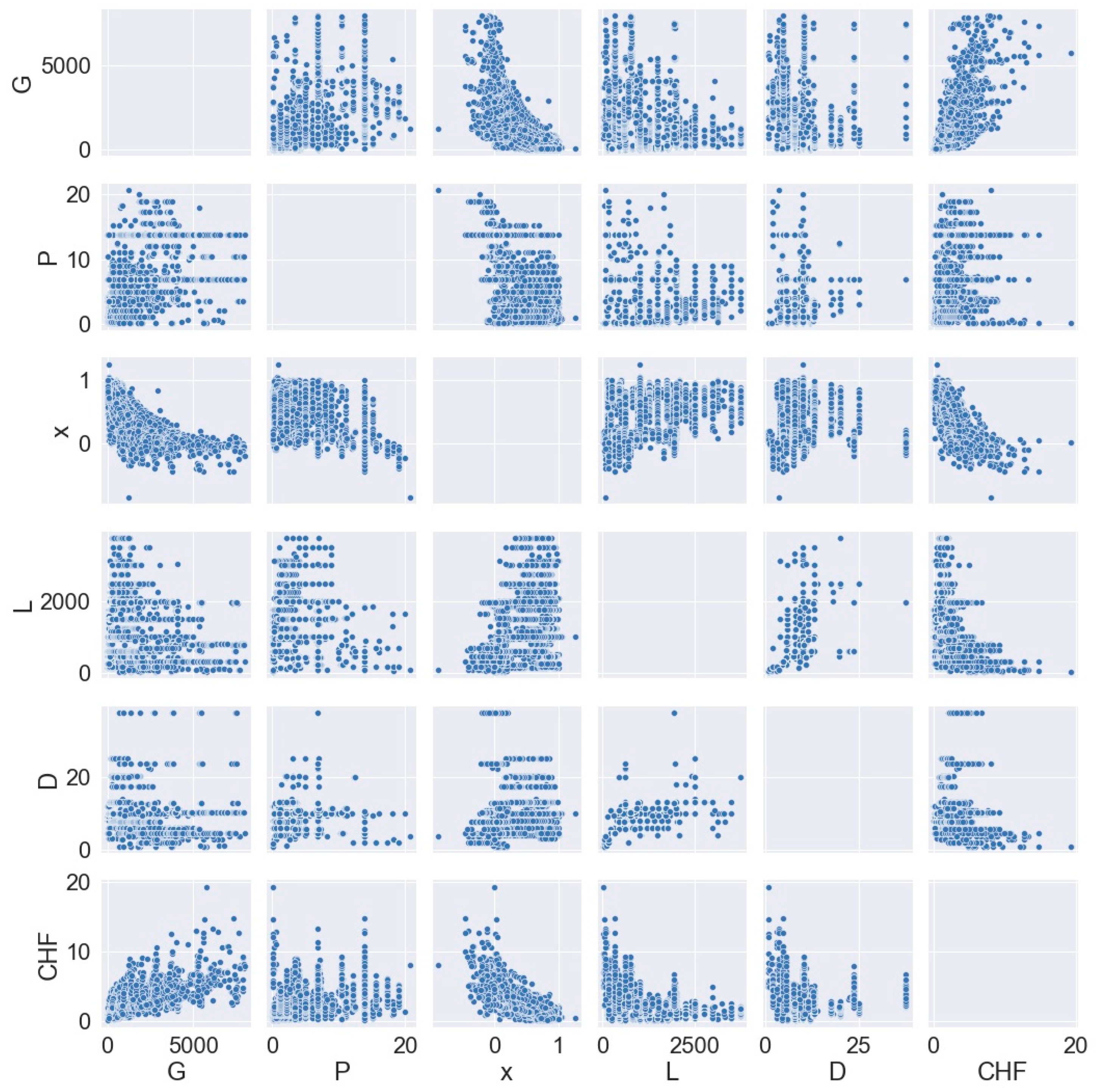
2.1. Dataset Generation

To construct the proposed framework, an extensive selection of non-proprietary experimental data on CHF available in the literature was utilized. The resulting dataset comprises 5877 samples, encompassing a wide range of system parameters, as demonstrated by the asymmetric distribution shown in Figure 1. The dataset encompasses both geometric and hydraulic features, with input variables obtained from the raw data including pressure (P), mass flux (G), tube equivalent diameter (D), local equilibrium/exit quality (x), and heated length (L). The output to be predicted is CHF, under the assumption that the distribution of heat flux along the axial direction is consistent or uniform.

Table 1. Experimental ranges of CHF Dataset.

Author	Mass-Flux (G) [kg/m2s]	Pressure (P) [MPa]	Equilibrium Quality (x) [-]	Heated Length (L) [mm]	Heated Diameter (D) [mm]	CHF [MW/m2]	No. of Samples
Inasaka [46]	4300–6700	0.31–0.64	−0.11 to −0.05	100	3	7.3–12.8	6
Williams [47]	325–4683	2.7–15.2	−0.02 to 0.92	1840	9.5	0.39–4.1	129
Kim [48]	20–277	0.11–0.95	0.32 to 1.2	300–1770	6–12	0.12–1.6	512
Becker [49]	100–5450	0.22–9.9	0 to 0.99	400–3750	3.9–25	0.28–7.5	3473
Lowdermilk [50]	60–597	3.4	0.71 to 0.94	152	3	0.47–3.3	21
Clark [51]	28–102	3.4–13.8	0.66 to 0.99	239	4.6	0.23–1.2	67
Reynold [52]	1166–2889	3.6–10.7	0 to 0.47	229	4.6	3.6–9	67
Peskov [53]	750–5361	10–20	−0.23 to 0.13	400–1650	10	0.9–4.3	17
Thompson [54]	542–7975	0.1–20.7	−0.86 to 0.21	25–3048	1–37.5	1–19.3	1585
Total	20–7975	0.1–20.7	−0.86 to 1.2	25–3750	1–37.5	0.12–19.3	5877

provides a summary of the experimental ranges for the dataset. In order to improve prediction accuracy, input variables are standardized (i.e., normalized to have a mean of 0 and a variance of 1).

2.2. Methodology

2.2.1. Look-Up Table (LUT) Method

The nuclear thermal-hydraulics industry commonly utilizes LUTs to predict CHF. The LUT is a well-established and highly trusted method utilized in nuclear facility safety evaluations. Specifically, LUT is a standardized database created for an 8 mm water-cooled vertical round channel, which encompasses a vast range of over 30,000 data points. These data points cover a wide spectrum of mass fluxes (ranging from 0 to 8000 kg/m²s), pressures (ranging from 0 to 21 MPa), and local qualities (ranging from −0.50 to 0.90). This comprehensive and standardized database is specifically designed to support safe and reliable decision-making processes in a variety of contexts. The CHF LUT approach offers several benefits, including the ability to cater to a wide range of practical applications, ease of use, and the absence of iterative calculations required to predict CHF [15]. Groeneveld et al. [55] presented a general equation aimed at addressing the diameter correction of the tube. The equation is formulated as follows:

$$\frac{{\mathrm{C}\mathrm{H}\mathrm{F}}_{\mathrm{d}}}{{\mathrm{C}\mathrm{H}\mathrm{F}}_{\mathrm{d}=8}}={\left(\frac{8}{\mathrm{d}}\right)}^{0.5}$$

(1)

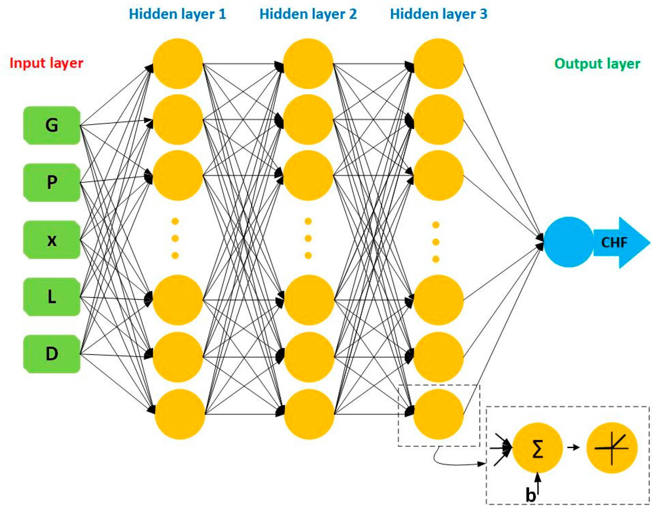
2.2.2. Artificial Neural Network (ANN)

ANN is a machine learning (ML) technique that is inspired by the functioning of the human brain. It comprises numerous processing units called neurons. The feed-forward neural network is the most widely used type of ANN in engineering today [56,57]. Typically, a neural network consists of three layers: the input layer, one or more hidden layers, and the output layer. A neural network is a type of machine learning model that is capable of learning both linear and non-linear patterns between the data [58]. It achieves this by incorporating several hidden layers and non-linear activation functions. During the training phase, the network’s accuracy is improved by adjusting the weights and biases of the neurons. This iterative process is known as learning, which involves minimizing the difference between expected and actual outputs. The weights and biases are randomly initialized, and the backpropagation learning technique is commonly used to adjust them. Neurons in each layer are connected to neurons in the next layer through weights, creating a complex network that can learn and make predictions. Each neuron has a threshold value, also called “bias”, employed to provide an extra degree of freedom. Inputs are multiplied by their corresponding weights in ANN. These weighted values and the neurons’ bias are added together as follows:

$${\mathrm{Z}}_{\mathrm{k}}=\left(\sum _{\mathrm{j}=1}^{\mathrm{q}}{\mathrm{w}}_{\mathrm{k}\mathrm{j}}{\mathsf{x}}_{\mathsf{j}}\right)+{\mathsf{b}}_{\mathsf{k}}$$

(2)

$${\mathrm{a}}_{\mathrm{k}}=f\left({\mathrm{Z}}_{\mathrm{k}}\right)$$

(3)

where q represents the number of neurons in each layer and w_kj are their cross-ponding weights of the input vector x_j. Z and b reflect the total weighted inputs and the bias of node k, respectively. Then this information is passed through activation function f [59]. Figure 2 illustrates the architecture of the ANN.

2.2.3. Support Vector Regression (SVR)

SVR is a powerful supervised learning method that aims to find an optimal hyperplane in a higher-dimensional space. By transforming the input space into a higher-dimensional space, SVR can effectively separate the input variables into two distinct regions. This hyperplane, which is equivalent to a line in two dimensions, serves as the prediction space for regression tasks. When performing regression with SVR, the algorithm seeks to find the hyperplane that best fits the data. This hyperplane is determined by selecting the support vectors, which are the data points closest to the hyperplane. The point that reflects the prediction is the hyperplane point closest to the data point being predicted [60].

By selecting the support vectors closest to the hyperplane, SVR is able to make accurate predictions for new data points. The mathematical representation of SVR is shown in Equations (4) and (5). Additionally, SVR improves data representation using kernel functions such as polynomial, RBF, and sigmoid functions. Kernel is a function that is used to map the input data from the original feature space into a higher-dimensional space, where the data is more separable. The kernel function operates on the input data and returns a measure of similarity between two points in the transformed space.

$$w{}^T\mathrm{x}+\mathrm{b}=0$$

(4)

$$\underset{}{\psi (w,\mathrm{\xi })=\frac{1}{2}{‖w‖}^2+\mathrm{m}\mathrm{i}\mathrm{n}\mathrm{C}}{\displaystyle \sum _{\mathrm{i}}^{\mathrm{n}}{\mathrm{\xi }}_{\mathrm{i}}}$$

(5)

In Equation (4), an input instance is represented by x, where $w{}^T$ is weight vector orthogonal to the decision-plane and b is a bias. C is a hyperparameter that regulates model generalization and ${\xi }_{\mathrm{i}}$ is a slack variable that represents misclassifications [61]. Thus, SVR uses hyper-parameter C to draw an optimal decision plane by establishing trade-off between class separating distance and misclassification rate.

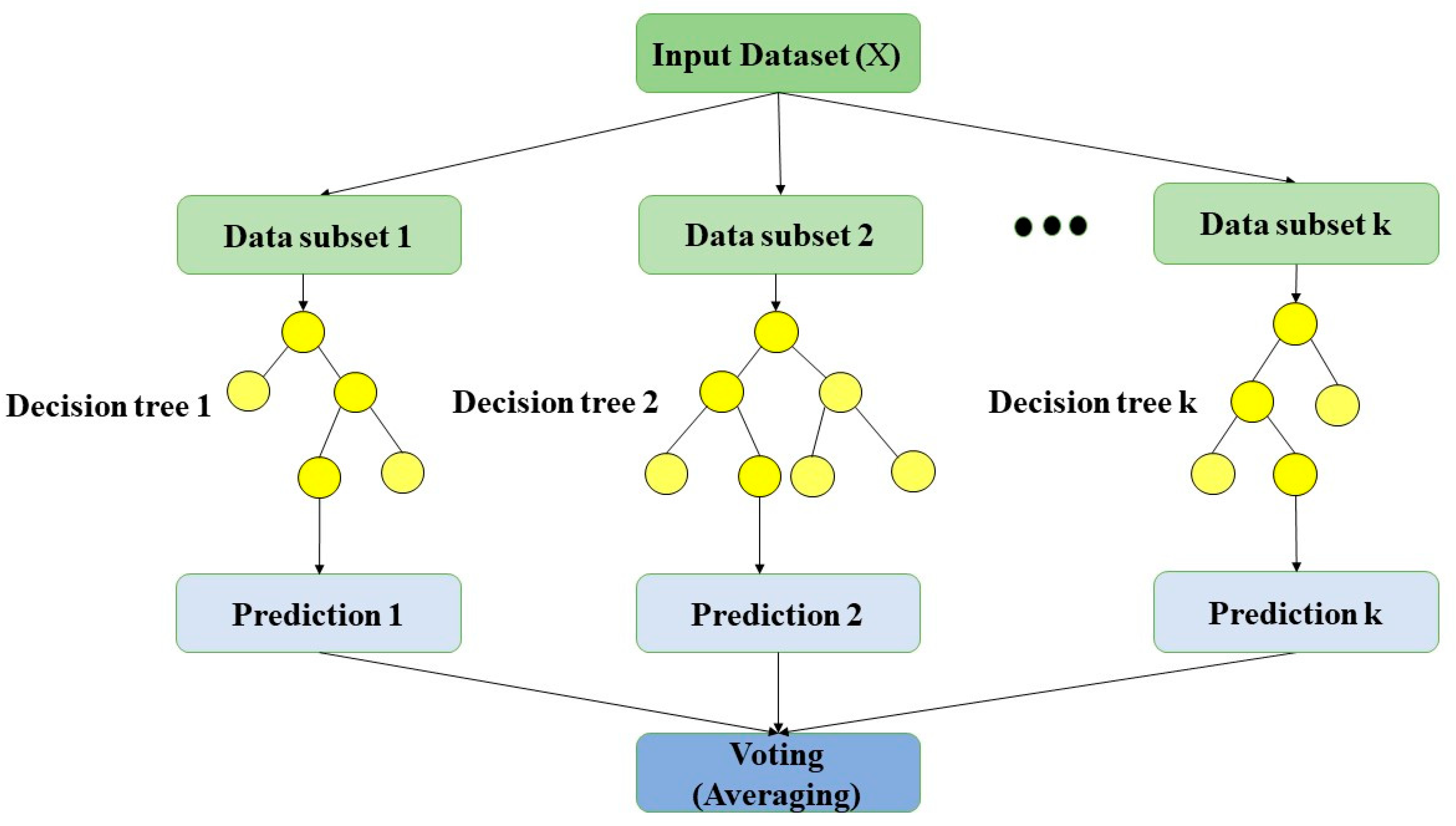
2.2.4. Random Forest (RF)

RF is a commonly employed ML technique for tackling regression problems. This technique is one of the most popular ensembles that employ a “bagging” method to enhance its resilience. The RF method employs ensemble learning, which involves combining multiple tree predictors to address complex problems. During training, RF modifies both the distribution of the input data and the features. Various subsets of data are used to train the number of tree predictors, and each internal tree predictor randomly chooses the subset of features used for data splitting. RF determines the outcome by taking the average of all predictions produced by the tree predictors [62]. The following equation represents the mathematical formula of RF used for regression.

$${\widehat{y}}^N\left(x\right)=\frac{1}{\mathrm{N}}\sum _{\mathrm{i}=1}^{\mathrm{N}}{y_{\mathrm{i}}\left(x\right)}_{}$$

(6)

where N represents total number of decision trees, ${y_{\mathrm{i}}\left(x\right)}_{}$ represents the ith decision tree on sample x from the dataset and ${\widehat{y}}^N\left(x\right)$ represents the average prediction of all decision trees. RF is considered to be the most prominent ensemble learning approach for producing reliable results with minimal hyperparameter tuning required. After generating individual predictions, the RF method utilizes the bagging technique, which aggregates results to increase accuracy, prevent overfitting, and minimize variance. Figure 3 demonstrates this process.

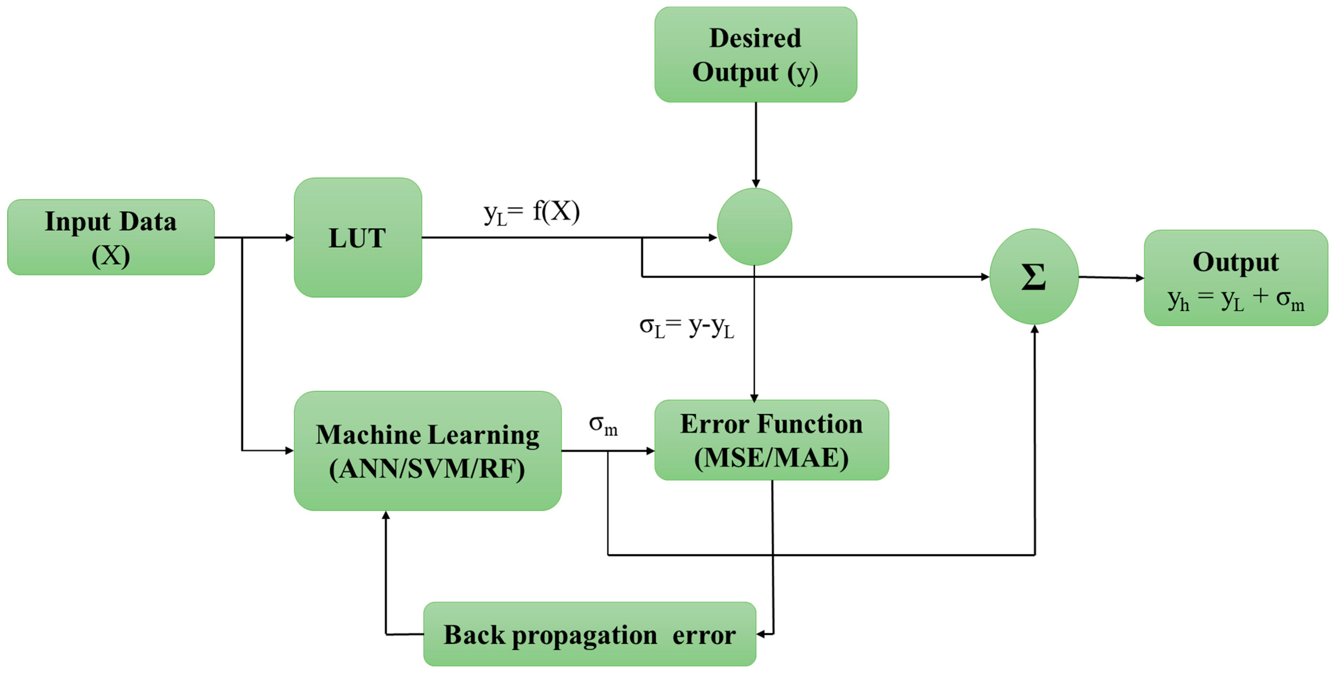
2.2.5. Data-Driven Hybrid Model

For the development of the proposed hybrid framework, the LUT is chosen as the prior model. In contrast to best-estimate standalone models, this hybrid framework utilizes a data-driven model as the foundation and offers a basic solution, while ML techniques are used to extract new knowledge from the discrepancy between the actual and anticipated result. For the prediction of CHF, input vector X consists of five variables, i.e., heated length (L), pressure (P), exit quality (x), mass flux (G), and equivalent diameter (D). Figure 4 depicts the flow of its training, validation, and testing methodology. The anticipated output (y_L) of the data-driven model is fundamentally a non-linear function of the input variables. During the learning process, as depicted in Figure 4, the error (σ) is calculated by subtracting y_L from the experimental output (y). The error (σ) obtained from the predicted values is utilized to train the ANN, SVR and RF. The predicted errors (σ_m) from ANN, SVR, and RF are compared with the error (σ) using an error/cost function. Typically, the loss function is presented in the form of mean absolute error (MAE) or mean squared error (MSE). The loss function is generally presented by MAE or MSE. The error function is optimized (minimized) during the learning/training process. The final prediction of the hybrid model y_h is the sum of y_L and σ_m. Relative root-mean-square error (rRMSE) is used to measure how well the hybrid model performs when evaluated against experimental results. The rRMSE is described as

$$\mathrm{r}\mathrm{R}\mathrm{M}\mathrm{S}\mathrm{E}=\sqrt{1/\mathrm{m}\sum _{i=1}^{\mathrm{m}}{\left(\frac{y_{\mathrm{i}}-y_{{\mathrm{h}}_{\mathrm{i}}}}{y_{\mathrm{i}}}\right)}^2}$$

(7)

where m represents datapoints. Similar to this, during the test phase, data-driven model and ML techniques (i.e., ANN, SVM and RF) are merged to obtain the expected output.

ML-based techniques have demonstrated clear advantages over LUT methods in a number of ways. One major advantage is that ML techniques require less prior knowledge and assumptions about the data being modeled. This is because ML algorithms are able to learn patterns and relationships directly from the data, rather than relying on preconceived notions about the underlying phenomena. One of the key benefits of these methods is their ability to extend the applicability domain online, which allows for continuous adaptation and improvement of the model. However, it is important to note that ML-based methods are purely data-driven, and their opaque properties can make it difficult to interpret the generated solutions. In addition, the models created by these methods can potentially produce widely dispersed and physically undesired solutions, especially when there is limited or noisy data available.

In this hybrid approach that relies on data, we go beyond relying solely on ML techniques and instead integrate prior knowledge to create more robust and reliable models that are suitable for diverse applications. By incorporating physical laws or constraints into the model, we can guide the learning process and reduce the likelihood of generating unrealistic solutions. This data-driven approach recognizes the value of prior knowledge and its potential to complement ML-based models. Combining these two approaches enables us to take advantage of the strengths of each and create more accurate and effective models. Moreover, incorporating prior knowledge can enhance the interpretability and transparency of the model, making it easier to understand and explain the results.

Ultimately, the integration of prior knowledge with ML techniques provides a comprehensive and effective solution to many real-world problems. By leveraging both data-driven and knowledge-driven approaches, we can improve the accuracy, reliability, and usefulness of our models.

3. Simulation Settings

ML algorithms are powerful tools for training and testing data in a variety of applications. ANN, SVR, and RF are some popular algorithms that can be used to accomplish this. To implement these algorithms, we can utilize the Keras application interface programming (API) backend provided by Tensorflow in conjunction with the sci-kit-learn library in Python 3.9. Before training and testing the data, it is essential to split the dataset into training and evaluation sets. Typically, we use 80% of the data for training and 20% for evaluating model performance. Moreover, we split the training dataset further into train and validation sets at an 80:20 ratio to select hyperparameters. The random distribution of the data ensures that the model performance can be assessed on unseen data. Hyperparameters play a crucial role in controlling the convergence and optimization of the ML models. When designing an ANN, the architecture is a critical aspect to consider. The design of a neural network’s architecture is critical for its ability to solve complex problems. This involves making several key decisions, such as selecting the appropriate number of hidden layers and neurons within each layer, choosing the activation functions used in each layer, setting the learning rate, and establishing the connections between the layers. To achieve accurate predictions and enable the network to generalize to new data, it is crucial to optimize the ANN’s architecture. This process involves selecting the optimal values for the architectural parameters and tuning them to maximize performance. By optimizing the ANN’s architecture, we can ensure that the network is capable of learning complex patterns and producing accurate predictions on both training and testing data. The physical parameters of the problem determine the number of neurons in the input and output layers. Hence, it is essential to select the appropriate number of neurons in the hidden layers, the activation function used in each layer, and the connections between the layers to achieve optimal performance. By carefully selecting hyperparameters and optimizing the ANN’s architecture, we can improve the accuracy of predictions and generalize well to new data.

Selecting the optimal topology for a neural network is a complex task and often requires a trial-and-error approach [63]. However, through experimentation, it has been found that a hybrid network architecture with three hidden layers yields optimal results. The three hidden layers contain 5/50/50/50/1 neurons as depicted in Figure 5, while a standalone ANN architecture has 5/100/100/100/50/1 neurons. The input layer comprises five neurons, corresponding to the input variables, while the output layer consists of one neuron.

To update the synaptic weights and biases, the Adam optimization algorithm with a learning rate of 0.001 is utilized. The Adam optimizer is particularly well-suited to deep learning problems and requires minimal tuning. It is a stochastic gradient descent optimization algorithm that is derived from an adaptive approximation of the first and second-order variables. The addition of non-linearity enhances the predictive capabilities of the model. Choosing the optimal topology for a neural network is a challenging task that involves many variables. However, through experimentation and optimization, it is possible to achieve a hybrid network architecture with three hidden layers that yields optimal results. By utilizing the Adam optimization algorithm with an appropriate learning rate, we can update the synaptic weights and biases of the model and enhance its predictive capabilities. Overall, these strategies can help to improve the accuracy and generalization of the neural network model.

The Rectified Linear Unit (ReLU) transfer function has gained popularity and is widely used in the hidden layers of the proposed model due to its excellent performance. ReLU is a universal approximator, meaning that it can estimate any function. In this study, ReLU outperformed sigmoid activation functions, making it the preferred choice for deep learning models. Compared to sigmoid, ReLU has several advantages that make it an attractive option. First, ReLU has a simpler computation process, which makes it faster to train ML-based neural networks. Additionally, ReLU allows for sparse activation, meaning that only a subset of neurons in a layer are activated, reducing the chances of overfitting. Furthermore, ReLU does not suffer from the vanishing gradient problem that can occur with sigmoid activation functions, which can lead to slow convergence during training.

The success of using ReLU activation functions in the hidden layers of the proposed model can be attributed to its universal approximation capabilities, faster training, sparse activation, and avoidance of the vanishing gradient problem. These advantages have resulted in improved performance compared to sigmoid activation functions in this study [64]. Therefore, ReLU is a promising activation function for deep learning models that can enhance their accuracy and efficiency.

When using SVR and RF algorithms, exploring hyperparameters is also necessary to achieve optimal performance. This involves carefully selecting values for various parameters to obtain the best possible results from these models. By fine-tuning hyperparameters, we can enhance the accuracy and efficiency of these algorithms in training and testing data, ultimately improving the overall performance of the models. For SVR, the optimal parameters are Kernel: Rbf, C: 100, and Nu: 0.9 (Kernel: Rbf, C: 100, Nu: 1 if using standalone SVR). On the other hand, the best RF model is determined to have 300 estimators/number of tree predictors (100 if using standalone RF).

Table 2. Configuration of CHF models.

Data-Driven Model	LUT
ML Approach	ANN, SVR, RF
Best-estimate ANN approach
▪ Network architecture	5/50/50/50/1 (5/100/100/100/50/1 if standalone ANN)
▪ Weight optimization algorithm	Adam
▪ Hidden layers activation function	ReLU (Rectified Linear unit)
▪ Learning rate	0.001
Best-estimate SVR approach
▪ Parameters	Kernel: Rbf, C: 100, Nu: 0.9 (Kernel: Rbf, C: 100, Nu: 1 if standalone SVR)
Best-estimate RF approach
▪ Number of estimators	100 (300 if standalone RF)

provides a summary of the CHF model configurations that were found to result in the highest accuracy during the learning process. It is significant to note that careful selection of hyperparameters is crucial for achieving optimal model performance for both SVR and RF algorithms.

4. Performance Evaluations

4.1. Standalone ML Models (ANN vs. SVM vs. RF vs. LUT)

This study employed four distinct methods to estimate CHF in nuclear reactors for safety assessment purposes. The first approach is the LUT method, which is widely used in the thermal-hydraulic community for predicting CHF during both reactor design and operation. The remaining three techniques are all ML-based, consisting of ANN, SVR, and RF. These ML approaches have gained popularity due to their ability to accurately model complex patterns and provide accurate predictions for a wide range of applications. By utilizing multiple approaches, this study aims to provide a comprehensive evaluation of the different techniques and their suitability for predicting CHF in nuclear reactors.

In Figure 6a,b, the performance of each of these four techniques is compared in terms of rRMSE. This analysis provides a comprehensive evaluation of the effectiveness of each approach and can be used to determine the optimal method for CHF prediction in nuclear reactor safety analysis.

In terms of adaptability and modeling simplicity, the standalone ML-based techniques outperform the traditional data-driven approach. Their continuous extension of the applicable domain is a fundamental advantage. However, these ML-based approaches are black-box in nature and could result in widely dispersed, physically unrealistic solutions. The presence of outliers in the dataset may be the main problem, or it may be that the train and test data do not have the same distribution of the data, which is a necessary condition for any useful validation or test solutions in ML. Using prior information reduces scatter significantly. ML approaches are then utilized to complement domain expertise and learn from the predictive discrepancy since domain knowledge is capable of providing reliable basis predictions.

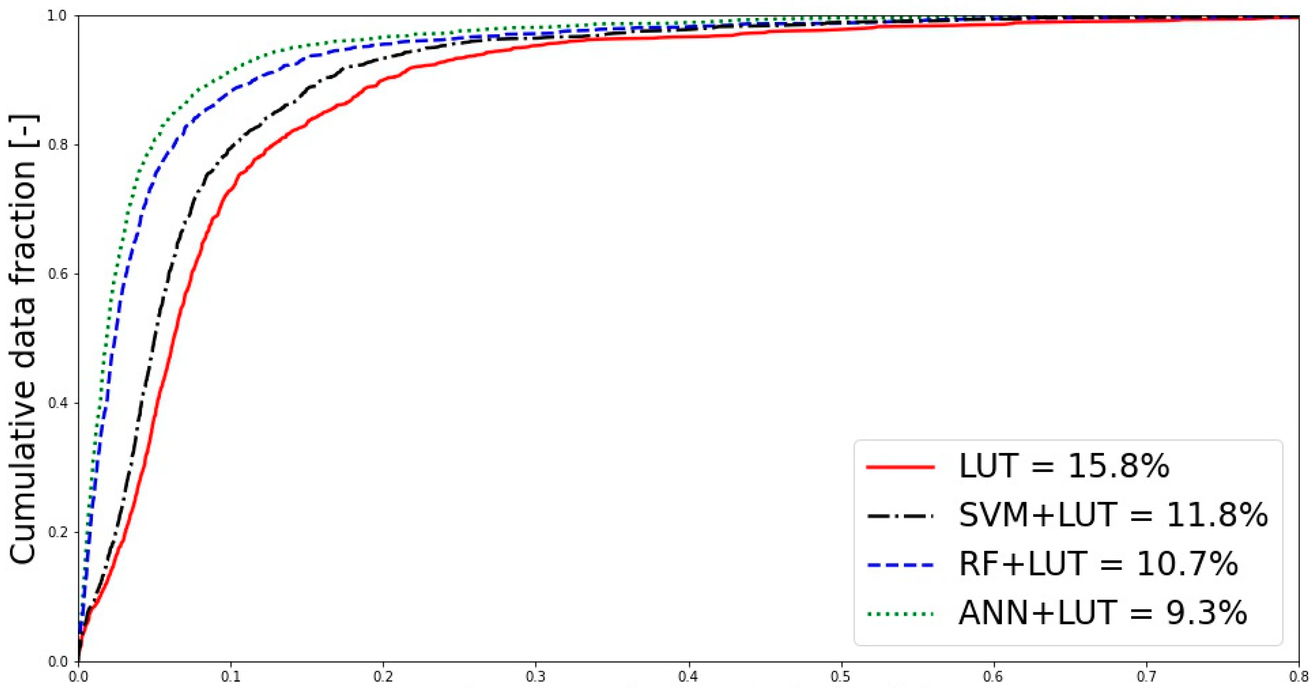
4.2. Comparison of Hybrid and Standalone Approaches

In this hybrid approach, the data-driven LUT is employed as the baseline model, and either ANN, SVM or RF can be used for ML. Hyperparameter tuning shows how well the ML structure can be optimized inside the hybrid model. For example, the ANN only needs three hidden layers with 50 neurons in each (5/50/50/50/1 structure) to perform at its best, while the RF only needs 100 tree predictors (instead of 300). The accuracy of standalone models (ANN, SVM and RF) vs. hybrid frameworks (ANN + LUT, SVM + LUT, RF + LUT) are depicted in Figure 7a–c). Compared to all standalone models, all hybrid model outperforms them as depicted in Figure 8. The rRMSE values of hybrid models are smaller than standalone models. The sharp rise in the curves between absolute-relative error and cumulative data fraction in hybrid models as compared to standalone models also depicts the superior predictive capabilities of the hybrid framework. The presence of a data-driven model provides the necessary setup for the hybrid “gray box”. Such a hybrid approach can use the prior model’s well-accepted physical rules and well-established empirical linkages to work in conjunction with ML.

Table 3. Different CHF models’ performance.

Approach	Test rRMSE (%)	Data-Points within ±10% Error	Data-Points within ±20% Error
LUT	15.8	68%	85%
SVM	15.5	72%	86%
RF	14.7	80%	89%
ANN	12.2	87%	95%
Hybrid SVM + LUT	11.8	87%	97%
Hybrid RF + LUT	10.7	89%	99%
Hybrid ANN + LUT	9.3	91%	100%

shows the performance of different CHF models. Absolute-relative deviation vs. data fraction of hybrid models (ANN + LUT, SVM + LUT, RF + LUT) is depicted in Figure 9. The comparison between the absolute relative error vs. data fraction curves of the ANN-based hybrid approach and the conventional LUT technique demonstrates a clear advantage for the former. The curve for the hybrid approach shows a marked increase in performance, whereas the curve for the LUT technique exhibits a less pronounced curve and inferior performance.

Furthermore, ML techniques also perform well compared to the LUT approach. However, the ANN-based hybrid approach outperforms as compared to ML techniques and the LUT approach, emerging as the clear winner. This is evidenced by a significantly smaller rRMSE of 9.3% and a faster rising cumulative data fraction curve, indicating fewer predictions that deviate from actual data.

In addition, the hybrid model (ANN + LUT) over the ranges of practical importance also corrects substantially distributed and biased parametric trends (CHF relative error vs. tube diameter, heated length, mass flowrate, pressure, exit quality) as depicted in Figure 10 using standalone LUT or ANN models. Such findings have further supported the hybrid approach’s improved generalization capacities.

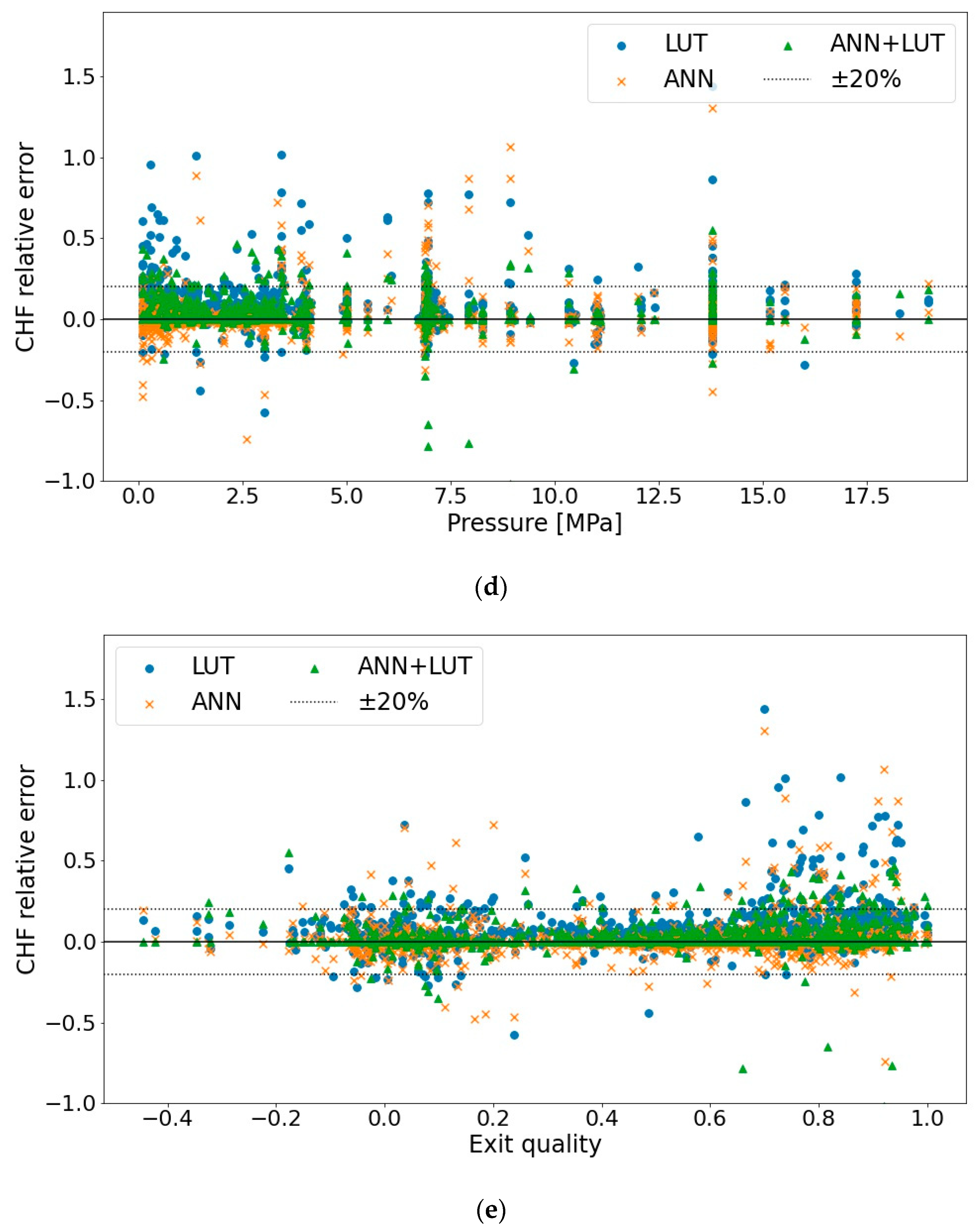
4.3. Sensitivity Analysis

To assess the effectiveness of the proposed hybrid model and to mitigate the risk of overfitting, k-fold cross-validation techniques are utilized. Most of the prior work for the prediction of CHF was based on hold-up cross-validation techniques [35,36,37,38,39,40,41,42,43,44,45]. The performance of the proposed hybrid model (LUT + ANN) of hold-up splits vs. k-fold cross-validation to further validate the model and to determine how well it generalizes to new data, as shown in

Table 4. Sensitivity analysis of the proposed hybrid model.

Sensitivity Analysis Technique	Test RMSE (%)	Test Samples within ±10% Error
80% train + 20% test	9.30	91%
5-fold cross-validation	9.15	89%
10-fold cross-validation	8.90	91%

. In 5-fold cross-validation, the data is divided into five subsets or folds, of which four subsets are used for training and one for testing. Similarly, this procedure is performed five times so that all data must pass through the test [65]. As the cross-validation technique produces more random splits, hence decreases the error produced due to bias. Although it increases the computational cost due to more random subsets are generated, but it is not our primary concern here as compared to desired accuracy due to critical nature of CHF prediction.

5. Conclusions

This study extends the prediction abilities of prior information and artificial intelligence (AI)-based techniques such as ML to enhance safety and financial profitability of heat transfer processes which depend on precise and reliable prediction of CHF by incorporating a data-driven hybrid model based on an ANN. The results of the comprehensive assessment have demonstrated that hybrid approaches based on artificial intelligence exhibit superior predictive capabilities when compared to the conventional LUT methods and standalone machine learning techniques that are commonly used. Furthermore, from this research work, we can conclude that:

○

The hybrid approach using ANN outperforms both traditional ML techniques and the conventional LUT technique when it comes to predicting accuracy.

○

Although standalone ML-based models performed better than the widely used conventional LUTs, the hybrid model greatly outperforms standalone ML models for prediction of CHF in vertical tubes for diverse set of operating parameters, with lower dispersion and non-biased parametric patterns.

○

ML architecture can be greatly simplified in the hybrid framework as compared to its standalone version to reduce computing costs when working with big databases.

○

From the parametric analysis in this work, it is confirmed that standalone ANN and hybrid (ANN + LUT) models have more suitable regression features between input and output than conventional LUT.

The results of this research offer valuable insights that can be leveraged to further develop and improve machine learning techniques, particularly deep learning models, for the prediction of CHF. The creation of a comprehensive database, as accomplished in this study, is critical for enhancing the accuracy and confidence of CHF predictions using machine learning approaches. With additional data, deep learning models can be trained to recognize more intricate patterns, leading to improved predictions and better understanding of the underlying physics. The findings of this research underscore the importance of continuous improvement and expansion of databases for developing and advancing machine learning models, which can benefit a diverse range of uses in the area of nuclear engineering and beyond. Expanding the range of input characteristics to include additional channel geometries can extend the utility of the developed models to other types of reactors. This research establishes a sturdy foundation for future investigations into CHF prediction using machine learning techniques. In conclusion, this study highlights the importance of exploring and including diverse input characteristics to improve the performance of ML-based CHF prediction models.

References

1. Pérez, F.I. Writing ‘usable’nuclear power plant (NPP) safety cases using bowtie methodology. Process Saf. Environ. Prot. 2021, 149, 850–857. [Google Scholar] [CrossRef]
2. Bruder, M.; Bloch, G.; Sattelmayer, T. Critical heat flux in flow boiling—Review of the current understanding and experimental approaches. Heat Transf. Eng. 2017, 38, 347–360. [Google Scholar] [CrossRef]
3. Baglietto, E.; Demarly, E.; Kommajosyula, R. Boiling crisis as the stability limit to wall heat partitioning. Appl. Phys. Lett. 2019, 114, 103701. [Google Scholar] [CrossRef]
4. Ghiaasiaan, S.M. Two-Phase Flow, Boiling, and Condensation: In Conventional and Miniature Systems; Cambridge University Press: Cambridge, UK, 2007. [Google Scholar]
5. Moreira, T.A.; Lee, D.; Anderson, M.H. Critical heat flux on zircaloy and accident tolerant fuel cladding under prototypical conditions of pressurized and boiling water reactors. Appl. Therm. Eng. 2022, 213, 118740. [Google Scholar] [CrossRef]
6. International Atomic Energy Agency. Operational Limits and Conditions and Operating Procedures for Research Reactors; Draft Safety Guide; International Atomic Energy Agency: Vienna, Austria, 2021. [Google Scholar]
7. Todreas, N.E.; Kazimi, M.S. Nuclear Systems Volume I: Thermal Hydraulic Fundamentals; CRC Press: Boca Raton, FL, USA, 2021. [Google Scholar]
8. Celata, G.P.; Cumo, M.; Mariani, A.; Simoncini, M.; Zummo, G. Rationalization of existing mechanistic models for the pre-diction of water subcooled flow boiling critical heat flux. Int. J. Heat Mass Transf. 1994, 37, 347–360. [Google Scholar] [CrossRef]
9. Bucci, M. Advanced diagnostics to resolve long-lasting controversies in boiling heat transfer. In Proceedings of the 13th In-ternational Conference on Heat Transfer, Fluid Mechanics and Thermodynamics, Portoroz, Slovenia, 17–19 July 2017. [Google Scholar]
10. Kandlikar, S.G. Critical heat flux in subcooled flow boiling—An assessment of current understanding and future directions for research. Multiph. Sci. Technol. 2001, 13, 26. [Google Scholar] [CrossRef] [Green Version]
11. Biasi, L.; Clerici, G.; Garribba, S.; Sala, R.; Tozzi, A. Studies on Burnout. Part a New Correlation for Round Ducts and Uniform Heating and Its Comparison with World Data; ARS, SpA and University of Milan: Milan, Italy, 1967. [Google Scholar]
12. Bowring, R. A Simple but Accurate Round Tube, Uniform Heat Flux, Dryout Correlation over the Pressure Range 0.7–17 MN/m2 (100–2500 PSIA); UKAEA Reactor Group: Oxfordshire, UK, 1972. [Google Scholar]
13. Tong, L. Heat transfer in water-cooled nuclear reactors. Nucl. Eng. Des. 1967, 6, 301–324. [Google Scholar] [CrossRef]
14. Katto, Y. A generalized correlation of critical heat flux for the forced convection boiling in vertical uniformly heated round tubes. Int. J. Heat Mass Transf. 1978, 21, 1527–1542. [Google Scholar] [CrossRef]
15. Groeneveld, D.; Shan, J.; Vasić, A.; Leung, L.; Durmayaz, A.; Yang, J.; Cheng, S.; Tanase, A. The 2006 CHF look-up table. Nucl. Eng. Des. 2007, 237, 1909–1922. [Google Scholar] [CrossRef]
16. Reddy, D. Parametric study of CHF data, volume 2, A generalized subchannel CHF correlation for PWR and BWR fuel assemblies. EPRI-NP-2609 1983, 2, 1983. [Google Scholar]
17. Tong, L.S.; Tang, Y.S. Boiling Heat Transfer and Two-Phase Flow; Routledge: Boca Raton, FL, USA, 2018. [Google Scholar] [CrossRef]
18. Xie, C.; Yuan, Z.; Wang, J. Artificial neural network-based nonlinear algebraic models for large eddy simulation of turbulence. Phys. Fluids 2020, 32, 115101. [Google Scholar] [CrossRef]
19. Abu Saleem, R.; Radaideh, M.I.; Kozlowski, T. Application of deep neural networks for high-dimensional large BWR core neutronics. Nucl. Eng. Technol. 2020, 52, 2709–2716. [Google Scholar] [CrossRef]
20. Hedayat, A.; Davilu, H.; Barfrosh, A.A.; Sepanloo, K. Estimation of research reactor core parameters using cascade feed forward artificial neural networks. Prog. Nucl. Energy 2009, 51, 709–718. [Google Scholar] [CrossRef]
21. Hedayat, A.; Davilu, H.; Barfrosh, A.A.; Sepanloo, K. Optimization of the core configuration design using a hybrid artificial intelligence algorithm for research reactors. Nucl. Eng. Des. 2009, 239, 2786–2799. [Google Scholar] [CrossRef]
22. Zubair, R.; Ullah, A.; Khan, A.; Inayat, M.H. Critical heat flux prediction for safety analysis of nuclear reactors using machine learning. In Proceedings of the 2022 19th International Bhurban Conference on Applied Sciences and Technology (IBCAST), Bhurban, Pakistan, 16–20 August 2022; pp. 314–318. [Google Scholar] [CrossRef]
23. Faria, E.F.; Pereira, C. Nuclear fuel loading pattern optimisation using a neural network. Ann. Nucl. Energy 2003, 30, 603–613. [Google Scholar] [CrossRef]
24. Kim, H.G.; Chang, S.H.; Lee, B.H. Optimal Fuel Loading Pattern Design Using an Artificial Neural Network and a Fuzzy Rule-Based System. Nucl. Sci. Eng. 1993, 115, 152–163. [Google Scholar] [CrossRef]
25. Desterro, F.S.; Santos, M.C.; Gomes, K.J.; Heimlich, A.; Schirru, R.; Pereira, C.M. Development of a Deep Rectifier Neural Network for dose prediction in nuclear emergencies with radioactive material releases. Prog. Nucl. Energy 2020, 118, 103110. [Google Scholar] [CrossRef]
26. Yong, S.; Linzi, Z. Robust deep auto-encoding network for real-time anomaly detection at nuclear power plants. Process. Saf. Environ. Prot. 2022, 163, 438–452. [Google Scholar] [CrossRef]
27. Saeed, H.A.; Peng, M.-J.; Wang, H.; Zhang, B.-W. Novel fault diagnosis scheme utilizing deep learning networks. Prog. Nucl. Energy 2020, 118, 103066. [Google Scholar] [CrossRef]
28. Guo, Z.; Wu, Z.; Liu, S.; Ma, X.; Wang, C.; Yan, D.; Niu, F. Defect detection of nuclear fuel assembly based on deep neural network. Ann. Nucl. Energy 2020, 137, 107078. [Google Scholar] [CrossRef]
29. Yiru, P.; Yichun, W.; Fanyu, W.; Yong, X.; Anhong, X.; Jian, L.; Junyi, Z. Safety analysis of signal quality bits in nuclear power plant distributed control systems based on system-theoretic process analysis method. Process. Saf. Environ. Prot. 2022, 164, 219–227. [Google Scholar] [CrossRef]
30. Bae, H.; Chun, S.-P.; Kim, S. Predictive Fault Detection and Diagnosis of Nuclear Power Plant Using the Two-Step Neural Network Models. Int. Symp. Neural Netw. 2006, 3973, 420–425. [Google Scholar] [CrossRef]
31. Adali, T.; Bakal, B.; Sönmez, M.; Fakory, R.; Tsaoi, C. Modeling nuclear reactor core dynamics with recurrent neural networks. Neurocomputing 1997, 15, 363–381. [Google Scholar] [CrossRef]
32. Koo, Y.D.; An, Y.J.; Kim, C.-H.; Na, M.G. Nuclear reactor vessel water level prediction during severe accidents using deep neural networks. Nucl. Eng. Technol. 2019, 51, 723–730. [Google Scholar] [CrossRef]
33. Bildirici, M.; Ersin, Ö.Ö. Regime-Switching Fractionally Integrated Asymmetric Power Neural Network Modeling of Nonlinear Contagion for Chaotic Oil and Precious Metal Volatilities. Fractal Fract. 2022, 6, 703. [Google Scholar] [CrossRef]
34. Bildirici, M.; Ersin, Ö. Markov-switching vector autoregressive neural networks and sensitivity analysis of environment, economic growth and petrol prices. Environ. Sci. Pollut. Res. 2018, 25, 31630–31655. [Google Scholar] [CrossRef]
35. Yapo, T. Prediction of critical heat fluex using a hybrid kohonen-backpropagation neural network. Intelligent Engineering Systems through Artificial Neural Networks-Proc. Artif. Neural Netw. Eng. (ANNIE’92) 1992, 2, 853–858. [Google Scholar]
36. Moon, S.K.; Baek, W.-P.; Chang, S.H. Parametric trends analysis of the critical heat flux based on artificial neural networks. Nucl. Eng. Des. 1996, 163, 29–49. [Google Scholar] [CrossRef]
37. Mazzola, A. Integrating artificial neural networks and empirical correlations for the prediction of water-subcooled critical heat flux. Rev. Générale Therm. 1997, 36, 799–806. [Google Scholar] [CrossRef]
38. Lee, Y.H.; Baek, W.-P.; Chang, S.H. A correction method for heated length effect in critical heat flux prediction. Nucl. Eng. Des. 2000, 199, 1–11. [Google Scholar] [CrossRef]
39. Kim, S.H.; Bang, I.-C.; Baek, W.-P.; Chang, S.H.; Moon, S.K. CHF detection using spationtemporal neural network and wavelet transform. Int. Commun. Heat Mass Transf. 2000, 27, 285–292. [Google Scholar] [CrossRef]
40. Su, G.; Fukuda, K.; Jia, D.; Morita, K. Application of an artificial neural network in reactor thermohydraulic problem: Prediction of critical heat flux. J. Nucl. Sci. Technol. 2002, 39, 564–571. [Google Scholar] [CrossRef]
41. Guanghui, S.; Morita, K.; Fukuda, K.; Pidduck, M.; Dounan, J.; Miettinen, J. Analysis of the critical heat flux in round vertical tubes under low pressure and flow oscillation conditions. Applications of artificial neural network. Nucl. Eng. Des. 2003, 220, 17–35. [Google Scholar] [CrossRef]
42. Zaferanlouei, S.; Rostamifard, D.; Setayeshi, S. Prediction of critical heat flux using ANFIS. Ann. Nucl. Energy 2010, 37, 813–821. [Google Scholar] [CrossRef]
43. Cong, T.; Chen, R.; Su, G.; Qiu, S.; Tian, W. Analysis of CHF in saturated forced convective boiling on a heated surface with impinging jets using artificial neural network and genetic algorithm. Nucl. Eng. Des. 2011, 241, 3945–3951. [Google Scholar] [CrossRef]
44. Jiang, B.; Zhao, F. Combination of support vector regression and artificial neural networks for prediction of critical heat flux. Int. J. Heat Mass Transf. 2013, 62, 481–494. [Google Scholar] [CrossRef]
45. Aldrees, A.; Awan, H.H.; Javed, M.F.; Mohamed, A.M. Prediction of water quality indexes with ensemble learners: Bagging and boosting. Process. Saf. Environ. Prot. 2022, 168, 344–361. [Google Scholar] [CrossRef]
46. Inasaka, F.; Nariai, H. Critical heat flux of subcooled flow boiling for water in uniformly heated straight tubes. Fusion Eng. Des. 1992, 19, 329–337. [Google Scholar] [CrossRef]
47. Williams, C.; Beus, S. Critical Heat Flux Experiments in a Circular Tube with Heavy Water and Light Water; AWBA Development Program; Bettis Atomic Power Lab.: West Mifflin, PA, USA, 1980. [Google Scholar] [CrossRef] [Green Version]
48. Kim, H.C.; Baek, W.-P.; Chang, S.H. Critical heat flux of water in vertical round tubes at low pressure and low flow conditions. Nucl. Eng. Des. 2000, 199, 49–73. [Google Scholar] [CrossRef]
49. Becker, K.M.; Hernborg, G.; Bode, M.; Eriksson, O. Burnout Data for Flow of Boiling Water in Vertical Round Ducts, Annuli and Rod Clusters; AB Atomenergi: Nyköping, Sweden, 1965. [Google Scholar]
50. Lowdermilk, W.H.; Weiland, W.F. Some Measurements of Boiling Burn-Out; National Advisory Committee for Aeronautics: Langley Field, VA, USA, 1955; Volume 16.
51. Clark, J.A.; Rohsenow, W.M. Local boiling heat transfer to water at low Reynolds numbers and high pressures. Trans. Am. Soc. Mech. Eng. 1954, 76, 553–561. [Google Scholar] [CrossRef]
52. Reynolds, J.M. Burnout in Forced Convection Nucleate Boiling of Water; Massachusetts Institute of Technology: Cambridge, MA, USA, 1957. [Google Scholar]
53. Peskov, O.; Subbotin, V.; Zenkevich, B.; Sergeyev, N. The critical heat flux for the flow of steam–water mixtures through pipes. In Problems of Heat Transfer and Hydraulics of Two Phase Media; Pergamon Press: Oxford, UK, 1969; pp. 48–62. [Google Scholar] [CrossRef]
54. Thompson, B.; Macbeth, R. Boiling Water Heat Transfer Burnout in Uniformly Heated round Tubes: A Compilation of World Data with Accurate Correlations; Reactor Group, United Kingdom Atomic Energy Authority: Oxfordshire, UK, 1964.
55. Tanase, A.; Cheng, S.; Groeneveld, D.; Shan, J. Diameter effect on critical heat flux. Nucl. Eng. Des. 2009, 239, 289–294. [Google Scholar] [CrossRef]
56. Ansari, H.; Zarei, M.; Sabbaghi, S.; Keshavarz, P. A new comprehensive model for relative viscosity of various nanofluids using feed-forward back-propagation MLP neural networks. Int. Commun. Heat Mass Transf. 2018, 91, 158–164. [Google Scholar] [CrossRef]
57. Qing, H.; Hamedi, S.; Eftekhari, S.A.; Alizadeh, S.; Toghraie, D.; Hekmatifar, M.; Ahmed, A.N.; Khan, A. A well-trained feed-forward perceptron Artificial Neural Network (ANN) for prediction the dynamic viscosity of Al2O3–MWCNT (40:60)-Oil SAE50 hybrid nano-lubricant at different volume fraction of nanoparticles, temperatures, and shear rates. Int. Commun. Heat Mass Transf. 2021, 128, 105624. [Google Scholar] [CrossRef]
58. Mohanraj, M.; Jayaraj, S.; Muraleedharan, C. Applications of artificial neural networks for refrigeration, air-conditioning and heat pump systems—A review. Renew. Sustain. Energy Rev. 2012, 16, 1340–1358. [Google Scholar] [CrossRef]
59. Haykin, S.; Network, N. A comprehensive foundation. Neural Netw. 2004, 2, 41. [Google Scholar]
60. Cortes, C.; Vapnik, V. Support-vector networks. Mach. Learn. 1995, 20, 273–297. [Google Scholar] [CrossRef]
61. Varol, Y.; Oztop, H.F.; Avci, E. Estimation of thermal and flow fields due to natural convection using support vector machines (SVM) in a porous cavity with discrete heat sources. Int. Commun. Heat Mass Transf. 2008, 35, 928–936. [Google Scholar] [CrossRef]
62. Kwon, B.; Ejaz, F.; Hwang, L.K. Machine learning for heat transfer correlations. Int. Commun. Heat Mass Transf. 2020, 116, 104694. [Google Scholar] [CrossRef]
63. Friedman, J.; Hastie, T.; Tibshirani, R. The Elements of Statistical Learning; Springer Series in Statistics; Springer: Cham, Switzerland, 2001; Volume 1. [Google Scholar]
64. Hanin, B. Universal Function Approximation by Deep Neural Nets with Bounded Width and ReLU Activations. Mathematics 2019, 7, 992. [Google Scholar] [CrossRef] [Green Version]
65. Li, K.-Q.; Liu, Y.; Kang, Q. Estimating the thermal conductivity of soils using six machine learning algorithms. Int. Commun. Heat Mass Transf. 2022, 136, 106139. [Google Scholar] [CrossRef]
Figure 1. Distribution of CHF dataset as function of two variables.
Energies 16 03182 g001
Figure 2. Architecture of ANN.
Energies 16 03182 g002
Figure 3. Architecture of RF.
Energies 16 03182 g003
Figure 4. Flow diagram of hybrid framework.
Energies 16 03182 g004
Figure 5. Architecture of ANN with 5/50/50/50/1 nodes used in optimal hybrid model.
Energies 16 03182 g005
Figure 6. (a,b). Experimental vs. predicated CHF for standalone best-estimate models (LUT vs. SVM vs. RF vs. ANN).
Energies 16 03182 g006
Figure 7. Absolute-relative deviation vs. data fraction of hybrid ANN+LUT (a), RF+LUT (b), SVM+LUT (c), and standalone ML models.
Energies 16 03182 g007
Figure 8. Test rRMSE of CHF models.
Energies 16 03182 g008
Figure 9. Absolute-relative deviation vs. data fraction of hybrid models.
Energies 16 03182 g009
Figure 10. CHF relative error distribution vs. tube diameter (a), heated length (b), mass flowrate (c), pressure (d), exit quality (e).
Energies 16 03182 g010aEnergies 16 03182 g010b