Renewable Scenario Generation Based on the Hybrid Genetic Algorithm with Variable Chromosome Length

Abstract

Determining the operation scenarios of renewable energies is important for power system dispatching. This paper proposes a renewable scenario generation method based on the hybrid genetic algorithm with variable chromosome length (HGAVCL). The discrete wavelet transform (DWT) is used to divide the original data into linear and fluctuant parts according to the length of time scales. The HGAVCL is designed to optimally divide the linear part into different time sections. Additionally, each time section is described by the autoregressive integrated moving average (ARIMA) model. With the consideration of temporal correlation, the Copula joint probability density function is established to model the fluctuant part. Based on the attained ARIMA model and joint probability density function, a number of data are generated by the Monte Carlo method, and the time autocorrelation, average offset rate, and climbing similarity indexes are established to assess the data quality of generated scenarios. A case study is conducted to verify the effectiveness of the proposed approach. The calculated time autocorrelation, average offset rate, and climbing similarity are 0.0515, 0.0396, and 0.9035, respectively, which shows the superior performance of the proposed approach.

1. Introduction

Renewable energy sources are fluctuant, stochastic, and uncontrollable [1,2]. The impact of large-scale renewable energy integration on the power system is becoming more and more obvious, and the risks of system operation are increasing [3,4,5]. The accurate scenarios of wind, solar, and load can provide the basis for power system dispatch and reduce the curtailment of renewable energies, which is significant for grid flexibility improvement [6,7]. The scenario generation methods can be classified into short-term, medium-term, and long-term methods, according to the length of time scale [8]. A probabilistic model of the dataset based on the Copula function is used to generate experimental scenarios that guarantee the autocorrelation of the data [9]. The literature [10] extracts key features of weather factors and uses the gated recurrent unit (GRU)-convolutional neural network (CNN) method to generate scenarios. The literature [11] utilizes the generative moment matching network (GMMN) and the optimization strategy to extract the typical wind power generation scenario. The wind and solar output probability densities are con-structed based on the non-parametric kernel density estimation and Frank-Copula functions, and the wind and solar scenarios are generated by using the spline interpolation method [12].

When modeling based on the time series analysis, the autocorrelation can provide enough information, and a high-accuracy model can be built based on the limited sample number of time series without the need to make predictions based on other conditions. The main methods for the analysis of time series are the wavelet analysis method [13], Kalman filter method [14,15], and autoregressive integrated moving average (ARIMA) model [16]. In [17], the ARIMA model and the identification of the model parameters are explained. The ARIMA model needs to be improved to adopt characteristics of wind, solar, and other renewable energies. The literature [18] combines the modified ensemble empirical mode decomposition (MEEMD) with the ARIMA model, and uses the MEEMD to process the data to improve accuracy. The literature [19] introduces frequency decomposition method to decompose the wind speed data and constructs the ARIMA model for the decomposed data. The non-smoothness factors of time series are eliminated by constructing seasonal-ARIMA based on stochastic probability analysis methods [20,21]. The literature [22] proposed a hybrid model of the ARIMA and triple exponential smoothing to achieve a real-time prediction of linear and nonlinear data. The literature [23] uses the combined method of wavelet transform and the ARIMA model to improve the accuracy of the ARIMA model. The data feature extraction method proposed in the literature [24] can capture data characteristics by using the correlation feature selection (CFS). The characteristics of the above methods are summarized in

Table 1. Characteristics of methods.

Literature	Model	Method of Data Analysis	Characteristic
[17]	ARIMA	None	Traditional Model
[18]	ARIMA	MEEMD	Expanding single-dimensional data to multidimensional
[19]	ARIMA	Frequency Decomposition	Determined cutoff frequency from experiments (complex processing)
[20,21]	ARIMA	None	Eliminate non-smoothness factors of time series
[22]	ARIMA and triple exponential smoothing	None	Improved ARIMA parameter determination method(small time overhead)
[23]	ARIMA	Wavelet Transform	Expanding single-dimensional data to multidimensional
[24]	Random Forest	CFS	Identify redundant data features

.

The accuracy of the scenario generation method is closely related to the dataset, and the analysis process of datasets is a nondeterministic polynomial (NP) problem. The NP problem can be solved using optimization algorithms, with the genetic algorithm (GA) being one of the key methods to solving the optimal problem. The traditional GA has defects, such as falling into local optimal solution and early convergence [25]. Many researches have been conducted to eliminate these defects. The search condition constraints are set up to improve the search speed of using GA to search for gene fragments [26]. The mixed-integer nonlinear programming (MINLP) is transformed into a linear programming problem by using the Chu–Beasley GA (CBGA) [27]. The literature [28] uses a pruning operator to improve the GA and increase the convergence of the algorithm. The literature [29,30] solve stochastic programming problems using GA. The former uses the biased random key genetic algorithm (BKAGA) and the latter uses the grid-oriented genetic algorithm (GOGA).

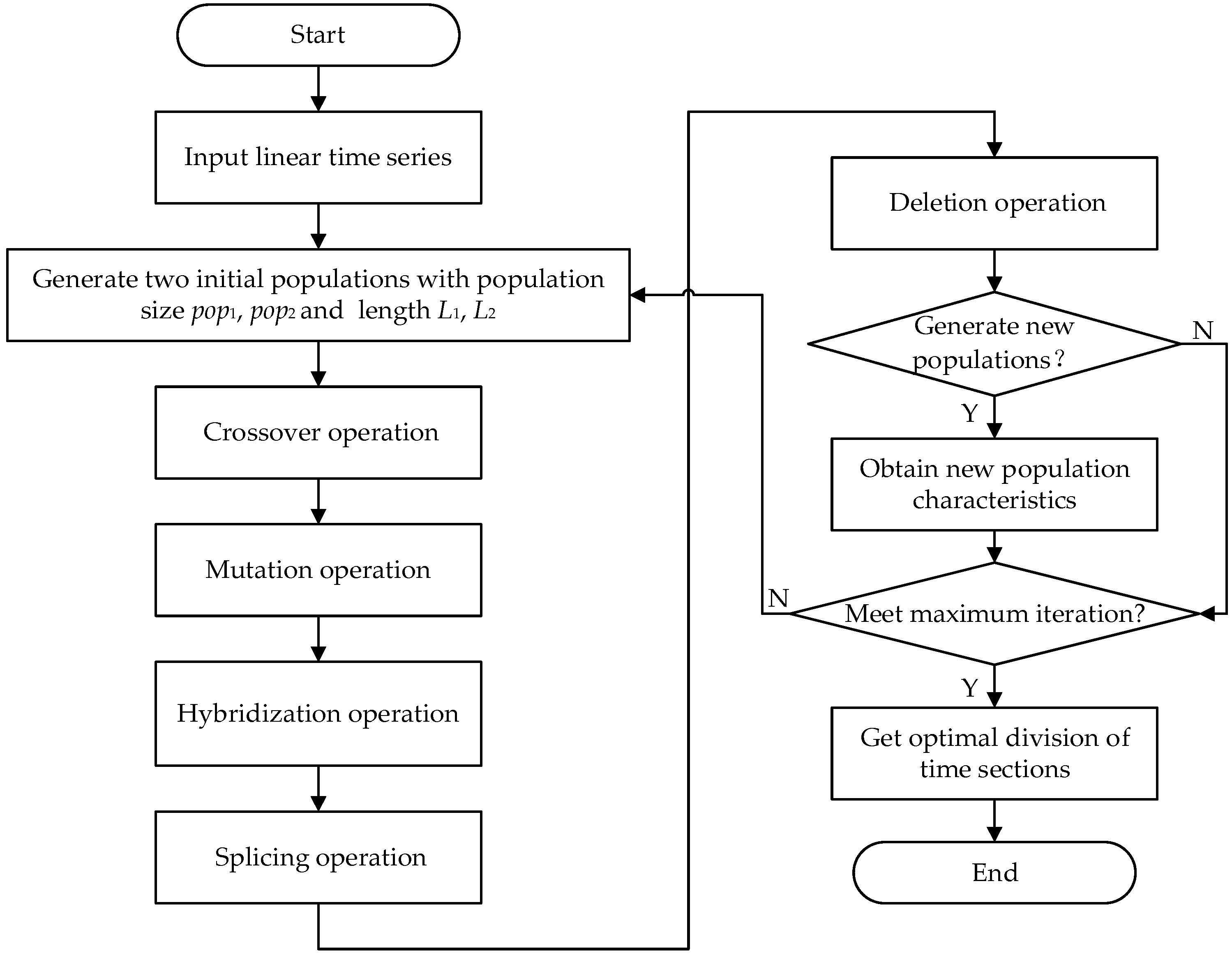
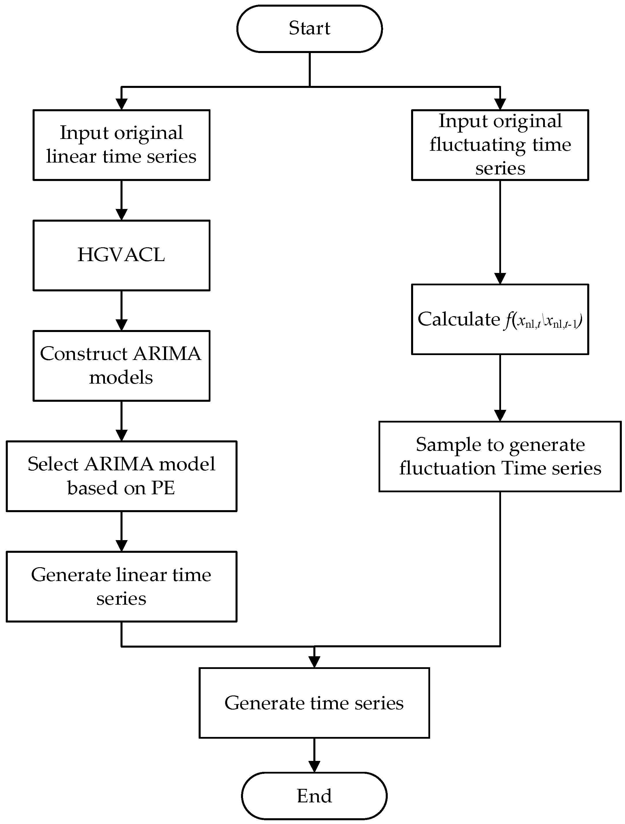
The above scenario generation methods also have defects, such as heavy calculation burden and complex calculation process. The complexity of the time series has an important impact on the scenario generation results. Therefore, this paper proposes a renewable scenario generation method that decomposes the original time series to decrease the complexity. The proposed approach can generate scenario results with a high amount of accuracy and has a superior performance in reflecting the characteristics of original data. The contributions can be listed as: (1) according to the time scales, the original data are divided into linear and fluctuant parts by the discrete wavelet transform (DWT); (2) a hybrid genetic algorithm with variable chromosome length (HGAVCL) is presented to optimally divide the linear part into different time sections; (3) the ARIMA model and Copula joint probability density function are, respectively, adopted to depict the linear and fluctuant parts.

The rest of this paper is organized as follows: Section 2 presents the decomposition of original time series. Additionally, the HGCVCL and renewable energy scenario generation method are presented in Section 3. Section 4 gives the steps of renewable energy scenario generation method and the assessment indexes. The case study is carried out in Section 5. Finally, conclusions are drawn in Section 6.

2. Decomposition of Time Series

2.1. Net Load Calculation

The power system with a high percentage of renewable energies have fluctuating characteristics, including the fluctuations of load and renewable generation. Therefore, the net load is used as the original time series and defined as,

$$P_{\mathrm{N}}=P_{\mathrm{L}}-P_{\mathrm{RES}}$$

(1)

where P_N is the power of net load; P_L is the power of load; and P_RES is the power of renewable generation.

2.2. Permutation Entropy of Time Series

Permutation entropy (PE) is used to measure the kinetic mutations and time series randomness, which can reflect the mutation of signals in a time series. PE has good robustness and is calculated quickly.

The time series {x_i, I = 1, 2, …, N} is reconstructed in phase space according to the PE and the reconstructed matrix is obtained as,

$$\left[\begin{array}{lllll}x\left(1\right)\hfill & \dots \hfill & x\left(1+i\tau \right)\hfill & \dots \hfill & x\left[1+\left(m-1\right)\tau \right]\hfill \\ \dots \hfill & \dots \hfill & \dots \hfill & \dots \hfill & \dots \hfill \\ x\left(j\right)\hfill & \dots \hfill & x\left(j+i\tau \right)\hfill & \dots \hfill & x\left[j+\left(m-1\right)\tau \right]\hfill \\ \dots \hfill & \dots \hfill & \dots \hfill & \dots \hfill & \dots \hfill \\ x\left(k\right)\hfill & \dots \hfill & x\left(k+i\tau \right)\hfill & \dots \hfill & x\left[k+\left(m-1\right)\tau \right]\hfill \end{array}\right]$$

(2)

where j = 1, 2, …, k; m is the embedding dimension; and τ is the delay time.

Each row of the reconstruction matrix arranged in ascending numerical order has a total of m! combinations and the PE is calculated as,

$$H_{\mathrm{p}}\left(m\right)=-{\displaystyle \sum _{i=1}^k{P}_i\ln \left(P_i\right)}$$

(3)

where P_i is the probability of occurrence of the i-th combination.

H_p(m) can quantitatively describe the complexity of the time series. The complex time series corresponds to large H_p(m) and simple time series corresponds to small H_p(m).

2.3. Time Series Decomposition Method

The original time series is decomposed into the low-frequency and the high-frequency parts using the discrete wavelet transform (DWT). The low-frequency series corresponds to the linear part and the high-frequency series corresponds to the fluctuant part. The linear series reflects the trend of the net load power in the scenario, and the fluctuating time series reflects the degree of variation in net load in the scenario.

The DWT can be expressed as,

$$W_f\left(p,r\right)=\langle f\left(t\right),{\psi }_{p,r}\left(t\right)\rangle ={\displaystyle {\int }_{-\infty }^{+\infty }f\left(t\right){\psi }_{p,r}^{*}\left(t\right)}dt$$

(4)

where f(t) is the original data function.

Linear series can be divided to reduce the complexity. Considering that PE can reflect the complexity of the time series, this paper transforms the linear time series partitioning problem into an optimization problem, where the objective function of the problem is to minimize the H_p(m). The control variables are the number of time sections and the length of each time section. The optimization problem is expressed as,

$$\min {\overline{H}}_p$$

(5)

$${\overline{H}}_{\mathrm{p}}=\frac{1}{n}{\displaystyle \sum _{z=1}^n{H}_{\mathrm{p}}\left(m_z\right)}$$

(6)

where n is the number of individual divided time sections; ${\overline{H}}_{\mathrm{p}}$ is the average H_p(m) of individual.

3. Principle of Scenario Generation Method

3.1. Hybrid Genetic Algorithm with Variable Chromosome Length

3.1.1. Framework of Proposed HGAVCL

For the problem of net load time series division, this paper proposes HGAVCL to improve the computational speed and accuracy, which has three parts:

(1)

Introduce hybridization operators, specify that the better individual perform hybridization with higher probability, and constrain the locations where chromosome segments can be hybridized.

(2)

Non-reproductive offspring produced is possible after the hybridization of organisms, and for this phenomenon, the survival factor ξ is proposed, which defines the survival probability of individuals after hybridization. The survival factor is calculated as,

$${\xi }_{b,a}=\frac{{\eta }_{b,a}}{{\eta }_{b-1,a,\min }}$$

(7)

where ξ_b,a is the survival factor of the a-th individual in the b-th generation; η_b,a is the fitness of the a-th individual in the b-th generation; and η_b−1,a,min is the minimum fitness of the a-th individual in the b−1-th generation.

Individuals with a survival factor greater than one are determined to be unable to reproduce offspring and unable to hybridize during the iterative calculation.

(3)

Considering the problem of time series division, the phenomenon of chromosome splicing and deletion exists in the process of biological inheritance. The chromosome splicing and deletion algorithms are proposed to realize the autonomous search for the number of the divided time sections.

3.1.2. Procedure of Proposed HGAVCL

The fitness of population individual i is expressed as,

$${\eta }_i={\overline{H}}_{\mathrm{p}}$$

(8)

The optimization problem is shown in (5), and the specific calculation procedure can be listed as:

(1)

The initial population I and II are set up based on the chromosome length. Based on a priori knowledge, the initial population I and II of individuals are selected. The length of population I chromosome is L₁ and the length of population II chromosome is L₂. The chromosome length represents the number of the divided time sections and the chromosomes are coded using binary. The sizes of population I and II are pop₁ and pop₂, respectively.

(2)

The new individuals are generated by the crossover operation with the crossover probability p_c.

(3)

The new individuals are generated by the mutation operation with the mutation probability p_v.

(4)

The hybridization operations are performed between populations according to the hybridization probability p_h, and if individuals are heritable based on growth factors, the new populations are generated.

(5)

The chromosome splicing is performed with splicing probability p_s. If the fitness of the spliced individual is greater than the lowest fitness individual in the previous generation, the individual is extinguished.

(6)

The chromosome deletion operation is performed with the deletion probability p_d. If the individual fitness is greater than that of the lowest fitness individual in the previous generation, the individual is extinguished.

(7)

The individual fitness of the population is calculated. The individuals of the population are selected via the Russian roulette method.

(8)

To ensure iterative convergence, the population extinction probability p_e is set. After each round of iterations, the population with the largest fitness among the best individuals of each population dies out with p_e.

(9)

Repeat the above steps (2)–(8) until the required number of iterations is satisfied.

(10)

The calculation process is shown in Figure 1.

3.2. Model of Linear Time Series

3.2.1. ARIMA Model

For ARIMA (p, d, q), the AR is the autoregressive and p is the number of autoregressive terms. The MA is the moving average and q is the number of moving average terms. The optimal number of differences to make it a smooth series is d [31]. The ARIMA model can be expressed as,

$$\left(1-{\displaystyle \sum _{i=1}^p{\phi }_i{B}^i}\right){\left(1-B\right)}^d{X}_t=\left(1+{\displaystyle \sum _{i=1}^q{\theta }_i{B}^i}\right){\epsilon }_t$$

(9)

$$B^p{X}_t=X_{t-p}$$

(10)

$${\nabla }^d{X}_t={\left(1-B\right)}^d{X}_t$$

(11)

where {X_t} is the time series; {ε_t} is normal white noise with mean 0 and variance 1; B is the backward shift operand; φ_i is the autoregressive coefficient; and θ_i is the moving average coefficient.

3.2.2. Parameter Calculation

The autoregressive parameter φ_i in the model can be determined by the autocorrelation coefficient ρ, i.e., the Yule–Walker equation, which can be expressed as,

$$\left[\begin{array}{c}{\phi }_1\\ {\phi }_2\\ ⋮\\ {\phi }_p\end{array}\right]={\left[\begin{array}{cccc}1& {\rho }_1& \cdots & {\rho }_{p-1}\\ {\rho }_1& 1& \cdots & {\rho }_{p-2}\\ ⋮& ⋮& \cdots & ⋮\\ {\rho }_{p-1}& {\rho }_{p-2}& \cdots & 1\end{array}\right]}^{-1}\left[\begin{array}{c}{\rho }_1\\ {\rho }_2\\ ⋮\\ {\rho }_p\end{array}\right]$$

(12)

The moving average parameter θ_i in the model can be determined by the self-covariance γ_k, which can be expressed as,

$${\gamma }_k=\{\begin{array}{ll}{\sigma }_{\epsilon }^2(1+{\theta }_1^2+{\theta }_2^2+\cdots +{\theta }_q^2)\hfill & k=0\hfill \\ {\sigma }_{\epsilon }^2(-{\theta }_k^2+{\theta }_1^2{\theta }_{k+1}^2+{\theta }_2^2+\cdots +{\theta }_q^2{\theta }_{q-k}^2)\hfill & 1\le k\le q\hfill \\ 0\hfill & k>q\hfill \end{array}$$

(13)

3.2.3. Augmented Dickey–Fuller

Augmented Dickey–Fuller (ADF) is used to determine the smoothness of time series. ADF is calculated as,

Model 1:

$$\Delta X_t=\alpha +\beta t+\delta X_{t-1}+{\displaystyle \sum _{i=1}^m{\beta }_i\Delta X_{t-i}}+{\epsilon }_t$$

(14)

Model 2:

$$\Delta X_t=\alpha +\delta X_{t-1}+{\displaystyle \sum _{i=1}^m{\beta }_i\Delta X_{t-i}}+{\epsilon }_t$$

(15)

Model 3:

$$\Delta X_t=\delta X_{t-1}+{\displaystyle \sum _{i=1}^m{\beta }_i\Delta X_{t-i}}+{\epsilon }_t$$

(16)

where ΔX_t is the residual at moment t; X_t−1 is the residual at moment t–−1; β_t is the coefficient of trend term; α is the constant; ε_t is the noise of residual.

The original hypotheses is H₀: δ = 0. The steps of calculation are in the order of model 1, model 2, and model 3. If the ADF rejects H₀: δ = 0 in any step of the ADF calculation, the original time series does not exist unit root, so it is a smooth time series, and the calculation is stopped. If the ADF satisfies H₀: δ = 0, the calculated ADF is finished with model 1, 2, and 3.

d is determined by ADF calculation. If the original time series is non-smooth, the calculation of difference needs to be continued. Otherwise, it is smooth and the calculation of difference is stopped.

3.2.4. Akaike’s Information Criterion

The autocorrelation coefficients and partial autocorrelation coefficients of the smooth series obtained after differencing do not have the characteristics of truncation. The p and q orders are determined by the Akaike’s information criterion (AIC).

AIC is calculated as,

$$\mathrm{AIC}(p,q)=\ln {\widehat{\sigma }}_x^2(p,q)+2(p+q)/T$$

(17)

The ${\widehat{\sigma }}_x^2$ is variance of model residuals, and expressed as

$${\widehat{\sigma }}_x^2(p,q)=\frac{{\displaystyle \sum _{t=1}^T\stackrel{⌢}{X}(t)}}{T-(p+q)}$$

(18)

where T is number of samples.

The ARIMA models are set up separately by different values of p and q taken from low-to-high order and the parameters are estimated. The results of each model AIC are compared. p₀ and q₀ are determined, which make the AIC extremely small. The p and q of the ARIMA model are p₀ and q₀, respectively.

The ARIMA models are constructed for the divided time sections to obtain the linear time series of the scenario.

3.3. Model of Fluctuant Time Series

3.3.1. Copula Function

The joint probability density model is developed by Copula function. Assuming the variables are [x₁, x₂, …, x_n], the joint distribution function is H(x₁, x₂, …, x_n), and the marginal distributions are [F₁, F₂, …, F_n], respectively, the Copula function is expressed as,

$$H(x_1,x_2,\dots ,x_n)=C(F_1(x_1),F_2(x_2),\dots ,F_n(x_n))$$

(19)

If F₁, F₂, …, F_n are continuous, C(F₁, F₂, …, F_n) is uniquely determined and the joint probability density function of the random vectors can be obtained by taking partial derivatives of both sides of (13).

$$h(x_1,x_2,\dots x_n)=c(F_1(x_1),F_2(x_2),\dots ,F_n(x_n)){\displaystyle \prod _{i=1}^n{f}_i(x_i)}$$

(20)

3.3.2. Copula Model Selection

This paper uses the Kendall coefficient and Spearman rank correlation coefficient as correlation evaluation pointers and calculates the Kendall coefficient and Spearman rank correlation coefficient of the simulated data generated by sampling based on the Copula function and the original data, respectively. If the correlation coefficients of the two are closer, the better the Copula function is fitted.

The Kendall coefficient ρ_τ is calculated as,

$${\rho }_{\mathsf{\tau }}=P\left[\left(V_1-V_2\right)\left(U_1-U_2\right)>0\right]-P\left[\left(V_1-V_2\right)\left(U_1-U_2\right)<0\right]$$

(21)

The Spearman rank correlation coefficient ρ_s is calculated as,

$${\rho }_{\mathrm{s}}=3\left\{P\left[\left(V_1-V_2\right)\left(U_1-U_3\right)>0-\left(V_1-V_2\right)\left(U_1-U_3\right)<0\right]\right\}$$

(22)

where (V₁, V₂) and (U₁, U₂) are random vectors having the same distribution that are independent of each other; P(∙) is its probability density function.

3.3.3. Fluctuant Series Model Construction

The net load fluctuation ratio x_nl,t is defined as,

$$x_{\mathrm{nl},t}=\frac{x_{\mathrm{nL},t}}{x_{\mathrm{L},t}}$$

(23)

The joint probability density function of net load fluctuating ratio to adjacent moment t and t − 1 is solved based on Copula theory.

$$h(x_{\mathrm{nl},t},x_{\mathrm{nl},t-1})=c(F_t,F_{t-1})\times f_k(x_{\mathrm{nl},t})\times f_{k+1}(x_{\mathrm{nl},t-1})$$

(24)

f(x_nl,t|x_nl,t−1) is solved based on the Bayesian formula and the probability model of the fluctuant part of scenario generation is obtained. The fluctuant time series is generated by sampling based on f(x_nl,t|x_nl,t−1). The results of our analysis show that the normal Copula function has superior performance.

4. Scenario Generation and Assessment

4.1. Scenario Generation Method

The computational process of the scenario generation method proposed in this paper is shown in Figure 2, and listed as follows:

(1)

Input the original linear time series and fluctuating time series.

(2)

Generate the linear time series scenario:

(1)

Divide zones based on HGAVGL.

(2)

Construct ARIMA model of each zone.

(3)

ARIMA model is selected based on PE to generate linear partial scenarios.

(3)

Generate fluctuating time series scenario:

(1)

Calculate f(x_nl,t|x_nl,t−1) based on Copula function.

(2)

Sample based on f(x_nl,t|x_nl,t−1) to generate fluctuating time series scenarios.

(4)

Combine linear and fluctuating time series to generate time series scenario.

Figure 2. Procedure of proposed scenario generation approach.

Figure 2. Procedure of proposed scenario generation approach.

4.2. Assessment Index

The generated scenarios characterize the uncertainty of the net load output and are time-dependent and consistent with the actual scenarios.

The time autocorrelation index σ, average offset rate index μ, climbing similarity index P_e, and mean absolute percentage error (MAPE) are adopted to assess the data quality of generated scenarios. The σ reflects the time correlation between the generated scenarios and the original scenarios. The μ reflects the offset degree between the generated scenarios and the actual running scenarios. The P_e reflects the climbing similarity between the generated scenarios and the original scenarios. Additionally, the MAPE reflects the accuracy of the ARIMA model.

(1)

Time autocorrelation σ

$$A_{\mathrm{time}}={|\mathrm{C}}_{\mathrm{history}}{-\mathrm{C}}_{\mathrm{gen}}|$$

(25)

$$\sigma =\frac{{\displaystyle \sum A_{ij}}}{L}$$

(26)

where A is the time autocorrelation approximation index matrix; C_history is the historical data time autocorrelation matrix; C_gen is the generated scenarios time autocorrelation matrix; i and j are adjacent moments, i.e., |i-j| = 1; and L is the scenarios length.

(2)

Average offset rate μ

$$\mu =\frac{1}{NT}{\displaystyle \sum _{t=1}^T{\displaystyle \sum _{j=1}^N\frac{\left|x_{j,t}-x_{\mathrm{history},t}\right|}{x_{\mathrm{history},t}}}}$$

(27)

where x_j,t is the net load value of the generated scenario at time t under the i-th generated scenario; x_history,t is the historical net load value at time t of the historical data; T is the generated scenario time stamp; and N is the number of simulations.

(3)

Climbing similarity P_e.

$$P_e=1-\frac{1}{\left(T-1\right)N}{\displaystyle \sum _{t=1}^T{\displaystyle \sum _{j=1}^N\frac{|\Delta c_{\mathrm{history},t+1,t}-\Delta c_{j,t+1,t}|}{x_{\mathrm{history},t}}}}$$

(28)

where Δc_{history,t+1,t} is the historical climbing value from moment t to moment t + 1; Δc_j,t+1,t is the generated scenario climbing value from moment t to moment t + 1.

(4)

MAPE

$$\mathrm{MAPE}=\frac{1}{l}{\displaystyle \sum _{c=1}^l\frac{|{\widehat{x}}_c-x_c|}{x_c}}$$

(29)

where ${\widehat{x}}_c$ is the predicted result at test set; x_c is the actual result at test set; l is the test set length.

5. Case Study

The minimum value of chromosome fragment length is 128. The value is determined by the experiment, which shows that 128 is the minimum to ensure the performance of solution algorithm. Additionally, the chromosome individual constraints are set up to ensure the accuracy of ARIMA model building. Two initial populations are set up. The population I with chromosome length is 5 and population II is 10. The number of iterations is 200, and the pop₁ and pop₂ are 40.

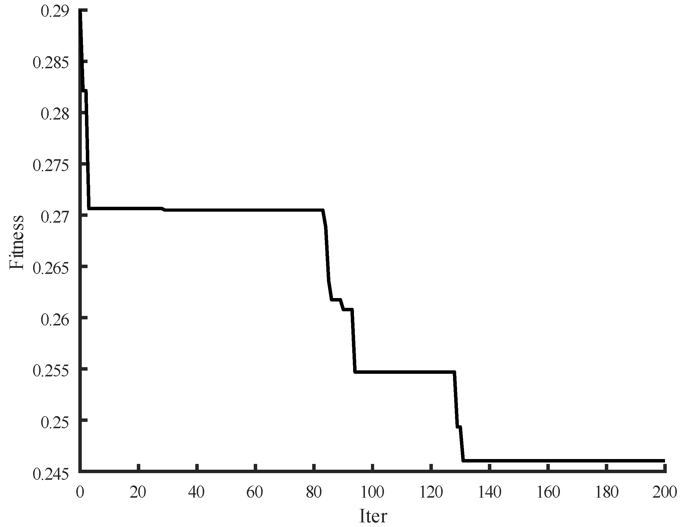
The PE of original linear time series is 3.46. Additionally, the PE is normalized and the value is 0.76. The fitness curve during the iterative process is shown in Figure 3.

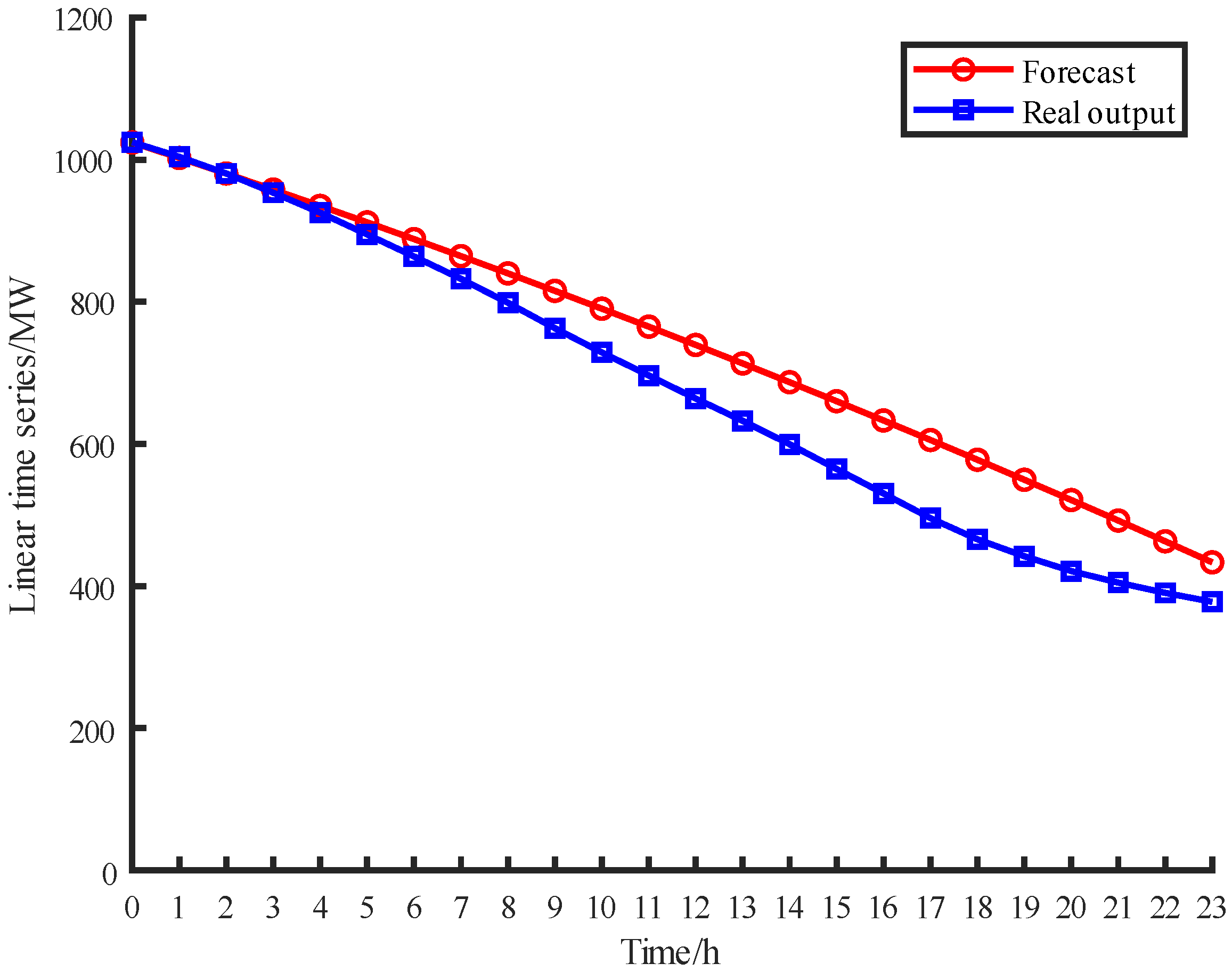
The results converge after 172 times and the chromosome length of optimal solution is 6. The original linear time series is divided into six zones. The ARIMA model is constructed for dividing the linear series. According to the existing research, the p and q orders of the ARIMA model are usually small, and this paper sets the maximum p and q order to 5. The fourth zone is analyzed as an example, and the construction series results of the ARIMA model are shown in Figure 4. The ADF results are shown in

Table 2. Results of ADF.

ADF	0	1
d	0	1

, and the AIC results are shown in

Table 3. Results of ADC.

AIC	p = 1	p = 2	p = 3	p = 4	p = 5
q = 1	−7049	−7075	−6850	−6809	−6807
q = 2	−6813	−6868	−7290	−6807	−6805
q = 3	−6811	−6866	−6807	−6805	−6803
q = 4	−7316	−6864	−6805	−6803	−6801
q = 5	−7241	−7253	−6746	−7132	−6902

. The ARIMA model parameters are shown in

Table 4. Parameter of ARIMA model.

Zone	p1	p2	p3	q1	q2	q3	d
Zone 1	0.23	0.13	0	−0.47	0	0	0
Zone 2	0.96	0	0	−0.34	−0.42	0	1
Zone 3	−0.14	0.35	0.51	−0.31	−0.08	−0.21	0
Zone 4	−0.47	−0.64	0	1.07	1.01	0.93	1
Zone 5	−0.07	0.18	0.29	−0.09	−0.91	0	1
Zone 6	−0.46	0.13	0.36	1.46	0.48	0	2

.

Additionally, the values of length, PE and MAPE of each time section, are shown in

Table 5. MAPE values and PE of each zone.

Zone	Length	MAPE	PE
Zone 1	751	0.1024	1.38
Zone 2	1832	0.0145	1.32
Zone 3	385	0.0514	1.28
Zone 4	629	0.0283	1.31
Zone 5	128	0.0283	0.29
Zone 6	5035	0.2229	1.42

. The results verify that the length of time sections affects the accuracy of the ARIMA model and the correlation between the distribution of PE and MAPE is positive. The smaller MAPE indicate that the constructed ARIMA is more accurate.

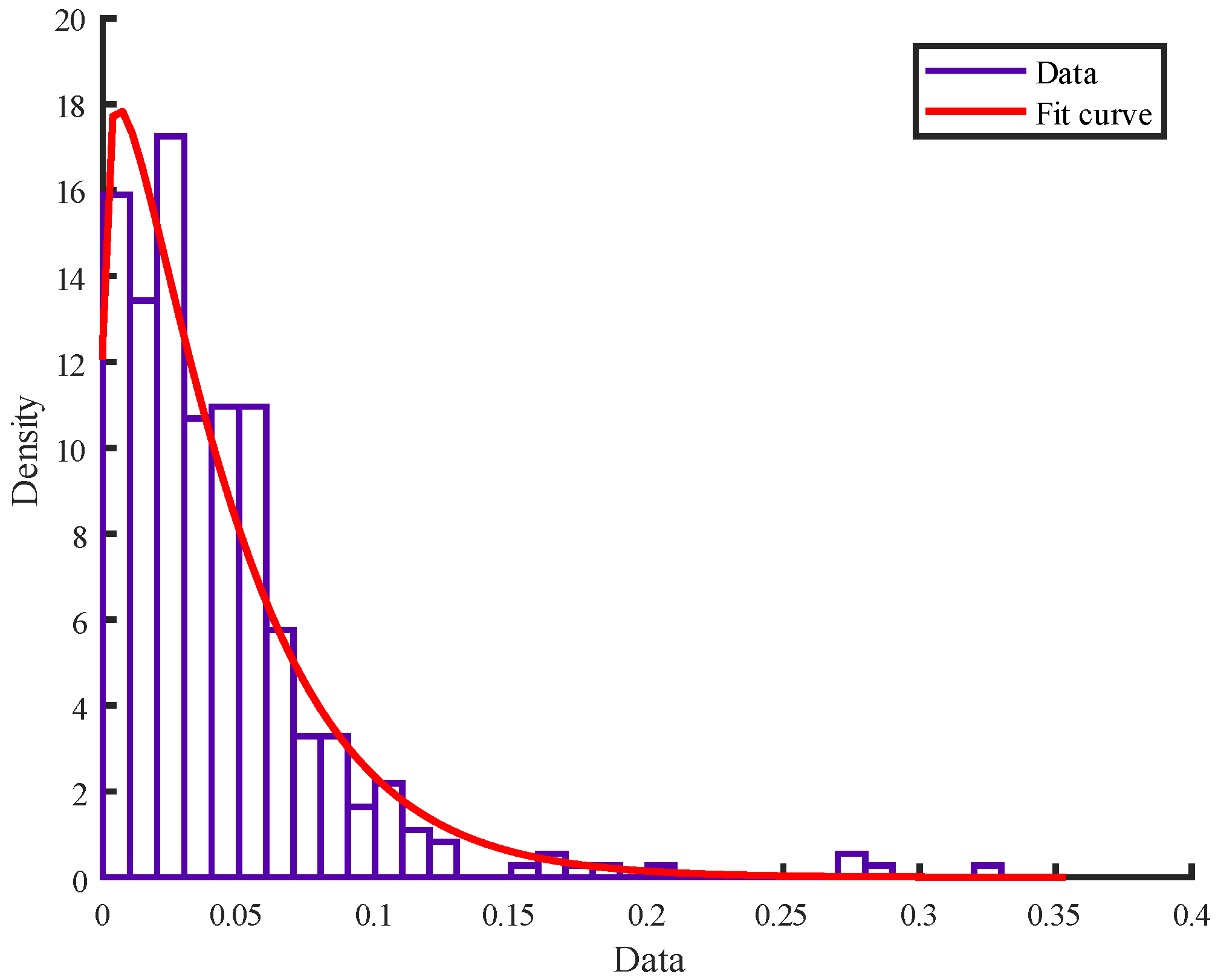
The value of net load ratio output at moment 1 and 2 is taken as an example, and the marginal distribution of net load ratio at moment 1 is shown in Figure 5. The marginal distribution is consistent with the Weibull distribution.

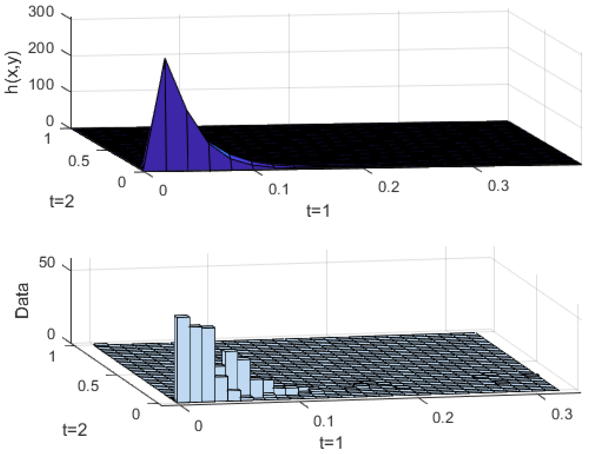
The Kendall correlation coefficient and Spearman rank correlation coefficient are used to compare the fitting effect of various types of Copula functions. The normal Copula function fitted well. Hence, it was used. The results are shown in Figure 6.

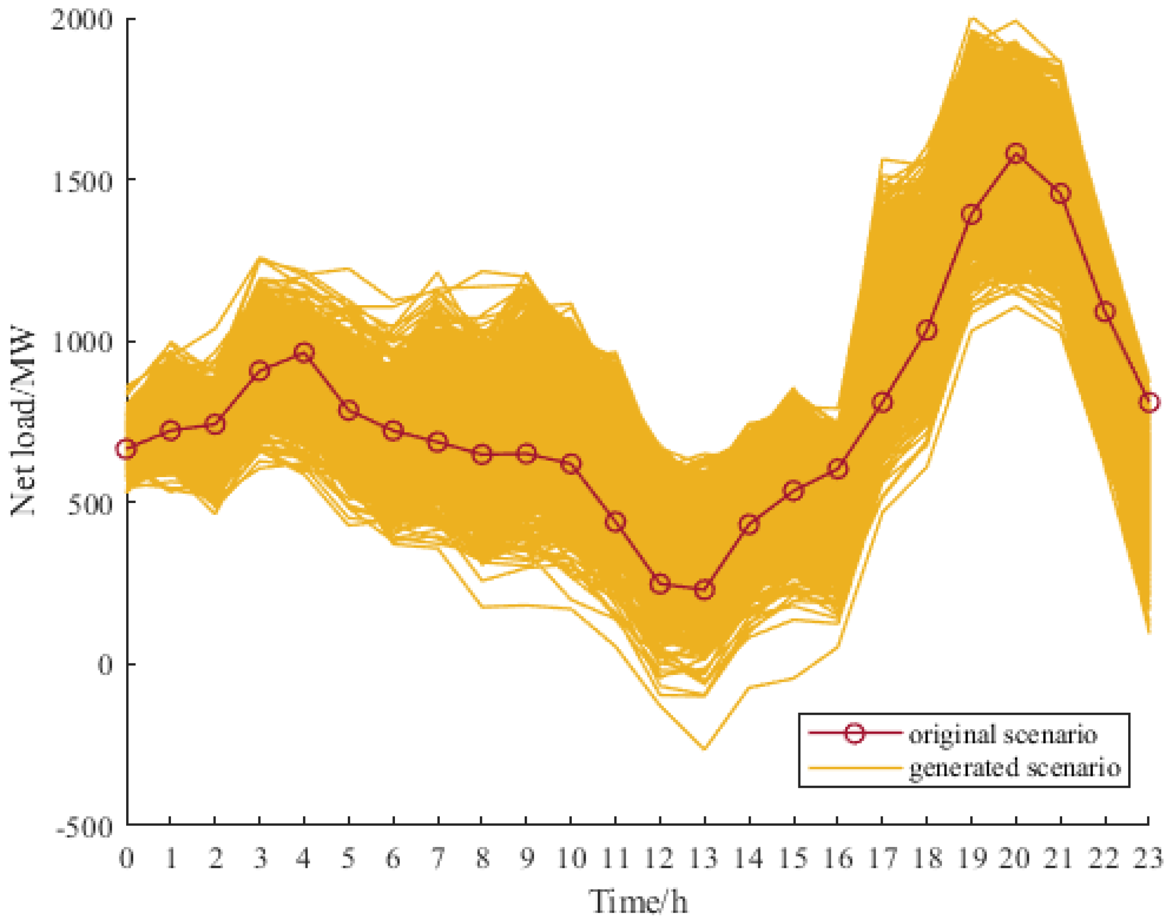
According to Figure 6, the shape of the fitted joint probability density is the same as the frequency histogram. The solutions of other adjacent moments joint probability densities are the same as in moment 1 and 2. The h(x,y) is solved according to the Bayesian formula to obtain the probability model of the fluctuant time series. The net load fluctuant time series is obtained based on the probability model. A set of scenarios are generated and shown in Figure 7.

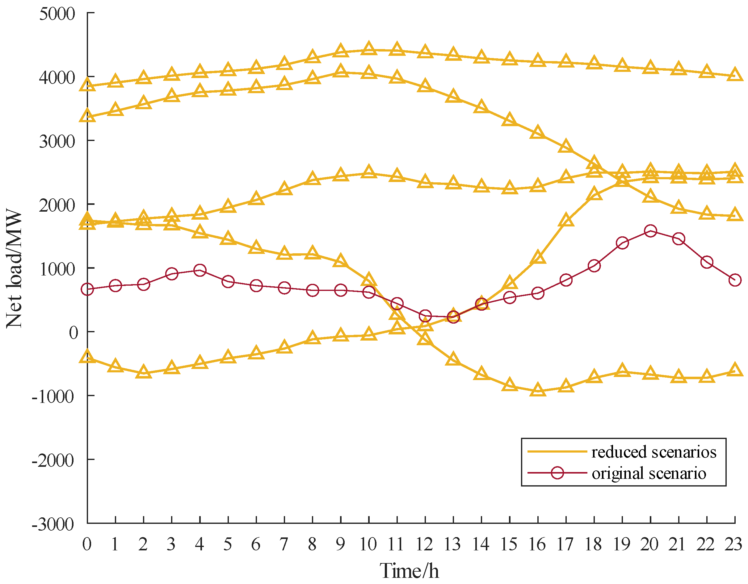
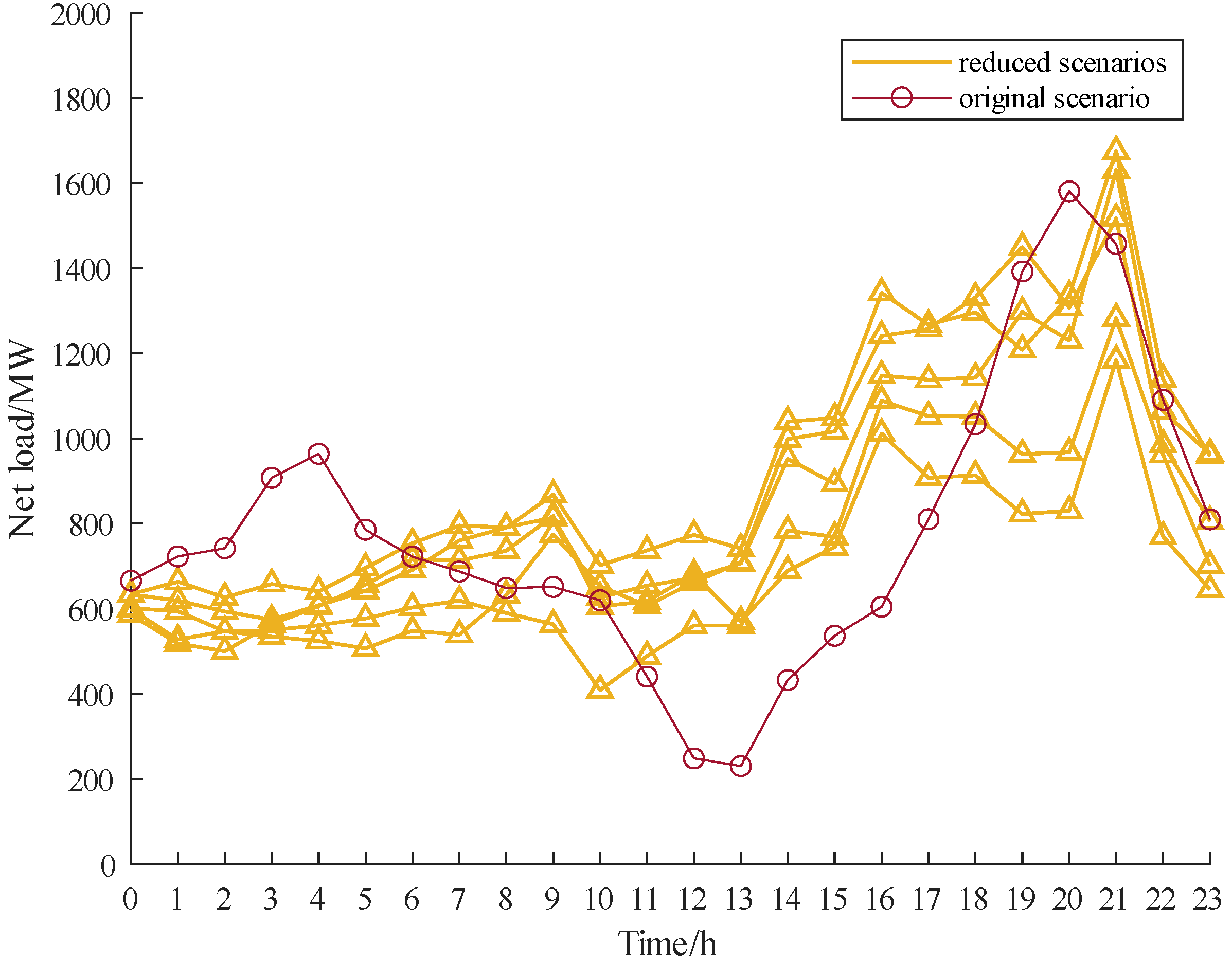
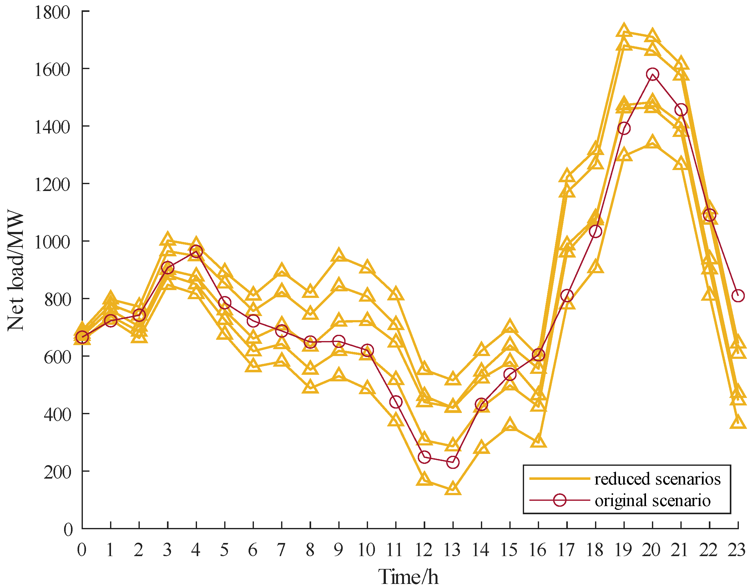
The Monte Carlo method, based on historical data, Copula function generation scenario method, and the proposed approach are compared. The number of generated scenarios is 1000. The k-means algorithm is used for scenario reduction and the results are shown in Figure 8, Figure 9 and Figure 10.

In order to illustrate the advantages of the proposed approach, the Monte Carlo sampling (MCS) method is carried out. The time autocorrelation σ, average offset rate μ, and climbing similarity P_e of the two methods are calculated, as shown in

Table 6. Results of evaluation indexes.

Method	Time Autocorrelation σ	Average Offset Rate μ	Climbing Similarity Pe
MCS method	0.0110	0.4673	0.8273
Proposed approach	0.0515	0.0396	0.9035

.

As for the time autocorrelation σ, the MCS method with the smaller value has little similarity to that of the generated and original data. In contrast, the proposed approach can better track the characteristics of original data. Additionally, Table 6 shows that the average offset rate μ of the proposed approach is smaller than the MCS method, which verifies the higher accuracy of the proposed approach. Furthermore, the proposed approach has better performance in climbing similarity P_e when compared to the MCS method. The scenarios generation method of Copula function satisfies the requirement of temporal correlation of adjacent moments and the requirement of climbing similarity, but the resultant offset of its generated scene is still not very satisfactory. Therefore, the proposed approach can generate scenario results with the highest amount of accuracy and the corresponding climbing similarity, which shows superior performance in reflecting the real situation of the net load scenario.

6. Conclusions

This paper proposes a renewable scenario generation approach based on the HGAVCL. With the use of the DWT, the original data are divided into the linear and fluctuant parts. For the linear part, the HGAVCL is used to minimize the PE and divide the time series into different time sections. This is modeled by the ARIMA. Additionally, the Copula joint probability density function is used to model the fluctuant part. The scenarios are generated by the Monte Carlo method, and the quantitative indices are established. The comparative analysis is conducted to demonstrate the advantages of the proposed approach. The proposed approach can improve the time autocorrelation σ and climbing similarity P_e, and reduce the average offset rate μ. The results show that the proposed approach better reflects the real situation of original data.

In future research, the optimal dispatching scheme for renewable energy sources, based on the proposed scenario generation approach, will be presented.

References

1. Cao, Y.; Wu, Q.; Zhang, H.; Li, C. Optimal Sizing of Hybrid Energy Storage System Considering Power Smoothing and Transient Frequency Regulation. Int. J. Electr. Power Energy Syst. 2022, 142, 108227. [Google Scholar] [CrossRef]
2. Chen, L.; Shen, J.; Zhou, B.; Wang, Q.; Buja, G. Quantitative Analysis on the Proportion of Renewable Energy Generation Based on Broadband Feature Extraction. Appl. Sci. 2022, 12, 11159. [Google Scholar]
3. Han, S.; He, M.; Zhao, Z.; Chen, D.; Xu, B.; Jurasz, J.; Liu, F.; Zheng, H. Overcoming the Uncertainty and Volatility of Wind Power: Day-Ahead Scheduling of Hydro-Wind Hybrid Power Generation System by Coordinating Power Regulation and Frequency Response Flexibility. Appl. Energy 2023, 333, 120555. [Google Scholar]
4. Xu, Q.; Cao, Y.; Zhang, H.; Zhang, W.; Terzija, V. Bi-Level Dispatch and Control Architecture for Power System in China based on Grid-Friendly Virtual Power Plant. Appl. Sci. 2021, 11, 1282. [Google Scholar] [CrossRef]
5. Cao, Y.; Wu, Q.; Zhang, H.; Li, C. Multi-Objective Optimal Siting and Sizing of BESS Considering Transient Frequency Deviation and Post-Disturbance Line Overload. Int. J. Electr. Power Energy Syst. 2023, 144, 108575. [Google Scholar]
6. Hu, J.; Li, H. A New Clustering Approach for Scenario Reduction in Multi-Stochastic Variable Programming. IEEE Trans. Power Syst. 2019, 34, 3813–3825. [Google Scholar] [CrossRef]
7. Wang, W.; Fang, X.; Cui, H.; Li, F.; Liu, Y.; Overbye, T.J. Transmission-and-Distribution Dynamic Co-Simulation Framework for Distributed Energy Resource Frequency Response. IEEE Trans. Smart Grid 2022, 13, 482–495. [Google Scholar]
8. Camal, S.; Teng, F.; Michiorri, A.; Kariniotakis, G.; Badesa, L. Scenario Generation of Aggregated Wind, Photovoltaics and Small Hydro Production for Power Systems Applications. Appl. Energy 2019, 242, 1396–1406. [Google Scholar] [CrossRef] [Green Version]
9. Nonvignon, T.Z.; Boucif, A.B.; Mhamed, M. A Copula-Based Attack Prediction Model for Vehicle-to-Grid Networks. Appl. Sci. 2022, 12, 3830. [Google Scholar] [CrossRef]
10. Li, H.; Ren, Z.; Xu, Y.; Li, W.; Hu, B. A Multi-Data Driven Hybrid Learning Method for Weekly Photovoltaic Power Scenario Forecast. IEEE Trans. Sustain. Energy 2022, 13, 91–100. [Google Scholar] [CrossRef]
11. Liao, W.; Yang, Z.; Chen, X.; Li, Y. Wind GMMN: Scenario Forecasting for Wind Power Using Generative Moment Matching Networks. IEEE Trans. Artif. Intell. 2022, 3, 843–850. [Google Scholar] [CrossRef]
12. Lin, S.; Liu, C.; Shen, Y.; Li, F.; Li, D.; Fu, Y. Stochastic Planning of Integrated Energy System via Frank-Copula Function and Scenario Reduction. IEEE Trans. Smart Grid 2022, 13, 202–212. [Google Scholar] [CrossRef]
13. Alves, D.K.; Ribeiro, R.L.; Costa, F.B.; Rocha, T.O.A. Real-Time Wavelet-Based Grid Impedance Estimation Method. IEEE Trans. Ind. Electron. 2019, 66, 8263–8265. [Google Scholar] [CrossRef]
14. Zhao, J.; Mili, L. A Decentralized H-Infinity Unscented Kalman Filter for Dynamic State Estimation Against Uncertainties. IEEE Trans. Smart Grid 2019, 10, 4870–4880. [Google Scholar] [CrossRef]
15. Mishra, C.; Vanfretti, L.; Jones, K.D. Synchrophasor Phase Angle Data Unwrapping Using an Unscented Kalman Filter. IEEE Trans. Power Syst. 2021, 36, 4868–4871. [Google Scholar] [CrossRef]
16. Liu, G. Time Series Forecasting via Learning Convolutionally Low-Rank Models. IEEE Trans. Inf. Theory 2022, 68, 3362–3380. [Google Scholar] [CrossRef]
17. Cardoso, C.A.V.; Cruz, G.L. Forecasting Natural Gas Consumption using ARIMA Models and Artificial Neural Networks. IEEE Lat. Am. Trans. 2016, 14, 2233–2238. [Google Scholar] [CrossRef]
18. Wu, F.; Jing, R.; Zhang, X.P.; Wang, F.; Bao, Y. A Combined Method of Improved Grey BP Neural Network and MEEMD-ARIMA for Day-Ahead Wave Energy Forecast. IEEE Trans. Sustain. Energy 2021, 12, 2404–2412. [Google Scholar] [CrossRef]
19. Yunus, K.; Thiringer, T.; Chen, P. ARIMA-Based Frequency-Decomposed Modeling of Wind Speed Time Series. IEEE Trans. Power Syst. 2016, 31, 2546–2556. [Google Scholar] [CrossRef]
20. Jafari, A.; Khalili, T.; Babaei, E.; Bidram, A.A. Hybrid Optimization Technique Using Exchange Market and Genetic Algorithms. IEEE Access 2020, 8, 2417–2427. [Google Scholar] [CrossRef]
21. Guo, J.; He, H.; Sun, C. ARIMA-Based Road Gradient and Vehicle Velocity Prediction for Hybrid Electric Vehicle Energy Management. IEEE Trans. Veh. Technol. 2019, 68, 5309–5320. [Google Scholar] [CrossRef]
22. Xie, Y.; Jin, M.; Zou, Z.; Xu, G.; Feng, D.; Liu, W.; Long, D. Real-Time Prediction of Docker Container Resource Load Based on a Hybrid Model of ARIMA and Triple Exponential Smoothing. IEEE Trans. Cloud Comput. 2022, 10, 1386–1401. [Google Scholar] [CrossRef]
23. Gangwar, P.; Mallick, A.; Chakrabarti, S.; Singh, S.N. Short-Term Forecasting-Based Network Reconfiguration for Unbalanced Distribution Systems With Distributed Generators. IEEE Trans. Ind. Inform. 2020, 16, 4378–4389. [Google Scholar] [CrossRef]
24. Mhawi, D.N.; Hashem, S.H. Proposed Hybrid Correlation Feature Selection Forest Panalized Attribute Approach to Advance IDSs. Karbala Int. J. Mod. Sci. 2021, 7, 405–420. [Google Scholar]
25. Montano, J.J.; Noreña, L.F.G.; Tobon, A.F.; Montoya, D.G. Estimation of the Parameters of the Mathematical Model of an Equivalent Diode of a Photovoltaic Panel Using a Continuous Genetic Algorithm. IEEE Lat. Am. Trans. 2022, 20, 616–623. [Google Scholar] [CrossRef]
26. Souza, M.G.; Vallejo, E.E.; Estrada, K. Detecting Clustered Independent Rare Variant Associations Using Genetic Algorithms. IEEE/ACM Trans. Comput. Biol. Bioinform. 2021, 18, 932–939. [Google Scholar] [CrossRef] [Green Version]
27. Huanca, D.H.; Pareja, L.A.G. Chu and Beasley Genetic Algorithm to Solve the Transmission Network Expansion Planning Problem Considering Active Power Losses. IEEE Lat. Am. Trans. 2021, 19, 1967–1975. [Google Scholar] [CrossRef]
28. Liu, Y.; Chen, X.; Zhao, Y. Joint Synchronization Estimation Based on Genetic Algorithm for OFDM/OQAM Systems. J. Syst. Eng. Electron. 2020, 31, 657–665. [Google Scholar]
29. Oliveira, B.B.; Carravilla, M.A.; Oliveira, J.F. A Diversity-Based Genetic Algorithm for Scenario Generation. Eur. J. Oper. Res. 2022, 299, 1128–1141. [Google Scholar] [CrossRef]
30. Kaushik, E.; Prakash, V.; Mahela, O.P.; Khan, B.; Abdelaziz, A.Y.; Hong, J.; Geem, Z.W. Optimal Placement of Renewable Energy Generators Using Grid-Oriented Genetic Algorithm for Loss Reduction and Flexibility Improvement. Energies 2022, 15, 1863. [Google Scholar] [CrossRef]
31. Ahmar, A.S.; Botto-Tobar, M.; Rahman, A.; Hidayat, R. Forecasting the Value of Oil and Gas Exports in Indonesia using ARIMA Box-Jenkins. J. Inf. Vis. 2022, 3, 35–42. [Google Scholar] [CrossRef]
Figure 1. Calculation process of proposed HGAVCL.
Energies 16 03180 g001
Figure 3. Iteration curve of fitness.
Energies 16 03180 g003
Figure 4. Results of ARIMA model.
Energies 16 03180 g004
Figure 5. Results of marginal distribution.
Energies 16 03180 g005
Figure 6. Results of Copula function.
Energies 16 03180 g006
Figure 7. Results of scenario generation.
Energies 16 03180 g007
Figure 8. Results of Monte Carlo method.
Energies 16 03180 g008
Figure 9. Results of Copula function generation scenario method.
Energies 16 03180 g009
Figure 10. Results of proposed approach.
Energies 16 03180 g010