A Comparative Parametric Study on Dynamic Biogenic Carbon of Harvested Wood Products: Biomass Rotation Period vs. Product Lifetime

Abstract

Harvested wood products (HWPs) are a class of products that are recognized for their potential to mitigate climate warming: the absorption of CO₂, which is necessary to the growth of their biomass feedstock, temporarily reduces the amount of CO₂ present in the Earth’s atmosphere, effectively mitigating global warming. This study decided to look into the effect of changing two important parameters associated with HWPs: the rotation period of the biomass used for their raw material (effectively, the rate of CO₂ absorption), and the length of their lifetime (effectively, the amount of time the captured carbon is stored within them in the form of embodied carbon). For this purpose, a carbon accounting calculator, Quantis’ Biogenic Carbon Footprint Calculator for Harvested Wood Products (BCFC-HWP), was employed. The Biogenic Global Warming Potential (GWP_bio) metric, which was used by the BCFC-HWP to describe the climate impact of a wooden product’s embodied carbon, was analyzed for its evolution with respect to the two identified parameters. The results showed that while GWP_bio followed a consistent decrease with respect to the product lifetime parameter, it showed a non-consistently evolving trend with respect to biomass rotation period i.e. first decreasing then increasing. This made the confrontation of both parameters’ effect complex mathematically, such that no clear-cut conclusions on the relative benefits of changing one parameter versus the other were made. Nonetheless, a valuable resolution was made based on the observations regarding the evolution of GWP_bio with respect to the lifetime of an HWP: the results indicated that extending the lifetime of an HWP is an advantageous strategy in decreasing the climate effect of the considered product.

1. Introduction

The potential of harvested wood products (HWP) in storing carbon and mitigating climate change has been widely recognized [1]. HWPs are estimated to represent a global carbon pool of 5 Gt in 2010, corresponding to 18.3 Gt CO₂. Furthermore, studies have estimated many European countries to have net negative emissions from HWPs with some showing down to −20 MtCO₂ per year [2].

Accurate estimating of the climate benefit of HWPs requires accurate accounting of temporality in biogenic carbon emissions. Various researchers throughout recent times have studied the potential of forest biomass as a mitigation strategy for global warming, both through wood energy products and medium- to long-lived wood products. Central to many of these works is the question of emissions timing and dynamic modeling of forest biogenic carbon, found to be an essential factor in painting an accurate picture of the climate benefits of HWP. The dynamics of the various forest carbon pools determines whether the forest acts as a source or sink for carbon. Thus, when estimating the GWP of a wooden product, the evolution of the amount of carbon contained within each forest carbon pool must be accurately accounted for. This is often conducted with the help of a software-based carbon stock modeling program, which estimates the exchanges of carbon across all forest carbon pools. These models are often themselves fed with information by dynamic growth model techniques [3], which they use to convert biomass into carbon removals and emissions [4].

The literature [5] has pointed out the limitations of using the typical Global Warming Potential (GWP) Characterization Factors (CF) in estimating the impacts of HWPs’ embodied biogenic carbon. Emitted amounts of biogenic carbon are always balanced, whether by prior or subsequent uptake depending on the chosen scenario. Under the GWP framework, this carbon neutrality equates to a climate neutrality where biogenic carbon appears as having no effect on the climate. Yet, researchers have pointed out that this assumption is often inaccurate [5,6,7]. One reason why the GWP of biogenic carbon always ends up at climate neutrality is the fact that this metric does not consider the timing of emissions within the analytical TH and is additionally unable to capture the temporal variability of the climate system’s response to emissions occurring at different times. A plethora of research studies in fields ranging from biofuels to construction materials have delved into the issue of time-sensitive accounting of biogenic carbon, some even attempting to develop more accurate indicators than GWP for the climate impact of these products [8,9,10].

In the 1990s, as interests in the potential climate change mitigation effects of the forestry sector grew, two notable works emerged as successful methods for incorporating time within carbon accounting calculations, the works of Moura-Costa et al. [11] and Lashof. [12]. These two studies focused on estimating the benefits that temporary carbon storage could offer to the warming of the climate. They both used a Mg-year approach, which consisted of considering the time-integrated abundance of a CO₂ emission in the atmosphere as representative of its climate effect. Moura-Costa et al. [11] then equated the time interval of integration to the necessary time period that a mitigation strategy must store carbon in order to have an equivalent (but negative) climate effect. Lashof et al. [12], in turn, considered that the benefits of carbon storage should be considered as an effective time delay in the emission, an approach which thereby consisted in subtracting the portion of the integral that is pushed outside the analytical time horizon once the delay is considered.

Following the early works of Moura-Costa [11] and Lashof [12], other researchers [9] during the 2010s looked into the topic of time-sensitive biogenic carbon accounting, due in particular to the emergence of biofuels. Kendall et al. [13] developed a time correction factor that corrected for amortization of LUC emissions throughout a biofuel lifecycle. O’Hare et al. [14] established the concept of fuel warming potential (FWP) with the same idea that LUC-related emissions cannot be allocated over the years of biofuel production.

Perhaps the two most notable works of this period are the respective studies by Levasseur et al. [15] and Cherubini et al. [16], whose methods for time-sensitive accounting of biogenic carbon stand out for their flexibility and their impact [17]. Levasseur’s work consisted of developing a general framework whereby time-specific emission profiles are used as the emissions inventory. Additionally, time-dependent GWP characterization factors are established to translate the emissions into accurate warming impacts, taking into account how long the emission has been present in the atmosphere. This method, named Dynamic LCA, is a generally applicable method, theoretically applicable for all LCA impact indicators; nonetheless, it remains very demanding in terms of data collection requirements.

Cherubini et al.’s [16] approach, on the other hand, focuses on biofuels and consists of developing a CF analogous to GWP but specific to biofuels. The basis for the work is the observation of a time gap between the time of carbon emissions during biofuel combustion and the re-sequestration of carbon through biomass regrowth; this time gap meant that, although biogenic carbon may be carbon neutral, it is not always climate neutral. The solution found was to directly integrate the process of carbon re-capture into the CF used to convert inventoried amounts of biogenic emissions into corresponding climate effects. This was conducted by using a different Impulse Response Function (IRF) to the one used for the traditional GWP: in their approach, the IRF used to calculate the Cumulative Radiative Forcing (CRF) of a biofuel accounts for the uptake of carbon not only in natural terrestrial/oceanic sinks but also the regrowth of replanted biomass. Thus, the climate effect of biofuels is no longer zero. Nonetheless, it remains inferior to the effect of an equivalent fossil emission because the CF used shows an accelerated decay for the CO₂ abundance. In other words, by this framework, biofuel emissions, rather than being considered as climate neutral, have simply lower impacts than fossil fuels.

In addition to the regrowth of merchantable stem wood, however, other carbon exchanges occur within the forest upon harvesting. These exchanges, which take place within the various carbon pools making up the forest stand, can contribute significantly to increasing the abundance of atmospheric CO₂ [4]. Incorporating these additional carbon exchanges within the GWP_bio framework was the basis of the work by Holtsmark et al. [18]. They adapted the GWP_bio metric in order for it to consider not only the recapture of carbon in the regrowth of biomass, but also the exchanges occurring within auxiliary carbon pools such as the soil and harvest residues. Holtsmark et al. [18] also proceeded to consider a no-harvest baseline scenario that serves as a benchmark against which carbon flows in the harvest scenario are measured. This allows for the climate effects of harvesting to be isolated from the effects which would have taken place regardless.

Further extensions were carried out on Cherubini’s GWP_bio concept in order to expand its scope of applicability to long-lived products. These are distinct from short-lived products such as biofuels in that they store carbon for a significant period of time before re-emitting it into the atmosphere. The original GWP_bio by Cherubini et al. [16] was designed specifically for biofuels: the mathematical expression describing it assumes that an initial emission of carbon is emitted into the atmosphere (before biomass and natural sink uptake); this assumption originates from the fact that biofuels are immediately oxidized back to CO₂ when used. Pingoud et al. [19] developed a GWP_bio,use term to account for the carbon credits which should be attributed to products that have a substantial lifetime and whose use cycle thereby includes the storage of carbon. In fact, they consider the climate benefits brought not only from further sequestering carbon during the product use cycle, but also consider benefits associated with the fact that a fossil equivalent of the product is displaced. Later, the work of Helin et al. [20] simplified Pingoud’s [19] approach by omitting the effect of product substitution and established a GWP_storage correction factor.

The abovementioned adaptations to GWP_bio form the basis of Quantis’ Biogenic Carbon Footprint Calculator for Harvest Wood Products (BCFC-HWP) [21]. Recently, a Wood Products Carbon Storage Estimator (WPsCS Estimator) [22], which includes the wood products’ disposal, recycling, and waste wood de-composition processes, has been applied to harvested wood products by Li et al. [23] and Zhao et al. [24]. However, to the best of the authors’ knowledge, no research paper has been published using BCFC-HWP. Therefore, the current research study looks to utilize the BCFC-HWP tool in order to observe the climate effects of changing two important aspects of an HWP lifecycle: the speed of ex-post carbon recapture, and the length of the period of carbon storage within the HWP. The role of the biomass rotation period has been highlighted in the literature e.g., [3,25,26,27,28,29,30]. More specifically, a recent publication by Guest et al. [25], carried out a similar study but used the original GWP_bio metric. Our study, by employing the BCFC-HWP, paints a more comprehensive and more accurate picture.

In fact, BCFC-HWP adopts the GWP_bio framework but includes carbon modeling within all forest carbon pools (estimated against a no-harvest scenario) and accounts for credits for carbon storage within HWP products. The flexibility of this calculator allows for an accurate estimation of the carbon footprint of various HWPs ranging from pulp and paper products to building materials. It accurately accounts for the time gap that exists between emissions and carbon recapture through biomass regrowth, all the while considering carbon storage within HWPs. In any case, it is important to note that the approach taken by Cherubini (and subsequent authors, all the way down to the BCFC-HWP) whereby biogenic carbon emissions are mitigated by the ex-post (i.e., after harvest) growth of biomass, is only one of two possible approaches to biogenic carbon accounting. The other, which considers ex-ante biomass growth, is more suitable for situations where biomass was purposefully grown for the intended HWP rather than situations as with the current one where the biomass that was harvested, was not intended for the produced HWP.

To achieve the aim of this study, a parameter analysis was carried out on the two following parameters: the biomass forest rotation period and the HWP product lifetime. This was conducted in order to answer the following research question: which strategy is the most effective in reducing the climate change effects of a HWP, reducing the time of ex-post carbon recapture in biomass or increasing the time of storage within anthroposphere? To present the results of this research question, the remainder of this paper will be organized into three parts: Section 2 where the workings of the BCFC-HWP tool will be detailed in order to understand how the two analyzed parameters were isolated and studied; Section 3 where the results of the analysis will then be presented and interpreted; and finally, Section 4 where the outcomes of the study will be summarized.

2. Methodology

2.1. BCFC-HWP Mathematical Model

The BCFC-HWP developed by Quantis [21] was the central tool used to carry out this study. Mobilizing a forest carbon growth model and the ecoinvent database, the calculator estimates the full lifecycle carbon footprint of a user-defined HWP. Calculations take into account both fossil and biogenic CO₂ emissions: the fossil emissions are linked to life cycle energy requirements for processing, transportation, distribution and storage, while the biogenic CO₂ emissions are those emanating from the embodied material of the HWP as it oxidizes. In addition, the model accounts for the temporary storage of carbon within HWPs. Thus, the main equation governing the workings of the calculator can be described with the following mathematical relation:

$${\mathrm{GW}}_{\mathrm{total}}={\mathrm{GWP}}_{\mathrm{bio},\mathrm{forest}}\times {\mathrm{C}}_{\mathrm{extracted}}\times (44/12)+\underset{\_}{{\mathrm{GWP}}_{\mathrm{bio},\mathrm{product}}\times {\mathrm{C}}_{\mathrm{product}}\times (44/12)}+{\mathrm{GW}}_{\mathrm{fossil}}$$

(1)

where:

-

GWP_bio,forest is an improved version of Cherubini et al.’s GWP_bio, where all carbon pools rather than just the merchantable stem wood are considered and evaluated with respect to a baseline no-harvest scenario. GWP _bio,forest mobilizes a forest growth model accounting for the temporal evolution of carbon within various forest carbon pools (specifically, vegetative biomass, dead organic matter biomass and soil organic carbon) upon harvest and operating in the background of the calculator.

-

C_extracted is carbon extracted from the forest.

-

GWP_bio,product is a term intended to adapt Cherubini’s original GWP such that it is also applicable for non-biofuel HWPs. This term subtracts a credit from the total GWP in order to compensate for the assumption within GWP_{bio, forest} that all harvested biomass is oxidized to CO₂ upon harvesting.

-

C_product is carbon stored in a product.

-

The 44/12 factor is the ratio of molecular weights between CO₂ and elemental carbon and is used to transform the biogenic GW into CO₂ equivalents.

-

m_{CO2, fossil} is the total mass of emitted fossil CO₂ emissions.

GWP is the traditional GWP factor.

It should be noted that a 100-year time horizon is applied.

For the purpose of understanding the current study, the mathematical modeling of GWP_bio,forest will be further detailed. GWP_bio,forest is calculated by integrating a function A(t) over the chosen analytical TH. A(t) is an analog to the traditional IRF(t) used for the calculation of CO₂’s CRF and GWP. A(t), however, is designed to describe the specific case of a HWP. In order to achieve this, it accounts for the time gap existing between CO₂ emissions from biofuel combustion and CO₂ recapture through ex-post tree planting. A(t) is based on Cherubini et al.’s [16] original f(t) which was a first modification to the IRF for CO₂ but designed only to incorporate the uptake of carbon via stem wood regrowth within the new IRF (in addition to the traditional uptake of carbon via natural terrestrial and oceanic sinks). Here, the BCFC-HWP’s A(t) builds upon f(t) by incorporating not just stem wood-related carbon uptake but carbon evolution within all forest carbon pools (that is, aboveground and belowground live biomass, dead organic matter and soil organic carbon). Mathematically, this is performed by computing the convolution of CO₂’s traditional IRF(t) with a function φ(t) which describes not only the regrowth of stem wood, but the total flux of carbon within the forest stand (φ(t) being obtained with the help of a dynamic carbon accounting software which models the evolution of carbon within forest carbon pools). In addition to correcting Cherubini et al.’s f(t) and accounting for all carbon stocks within a forest, A(t) also incorporates a comparison to a reference “no-harvest” scenario which allows it to isolate the climate effects due only to the harvesting process from those which would have occurred regardless. This is incorporated in the form of an additional term within the expression for A(t). Equations (2) and (3) represent Cherubini et al.’s model and the BCFC-HWP model, respectively.

$$f\left(t\right)={{\displaystyle \int }}_0^t\left[C_0·\delta \left(t^{\prime }\right)-g\left(t^{\prime }\right)\right]·y\left(t-t^{\prime }\right)d{t}^{\prime }$$

(2)

where:

• C₀ is the initial pulse emission of biogenic CO₂ into the atmosphere;
• δ(t) is the delta function (which is zero everywhere except for at origin);
• g(t) is the rate of biomass growth;
• y(t) is the fraction of the initial pulse still remaining at time t due to take-up in oceanic and terrestrial sinks.

$$A\left(t\right)={{\displaystyle \int }}_0^t\left[E\left(t,\sigma \right)·\delta \left(t^{\prime }\right)-{\phi }^{\prime }\left(t^{\prime }\right)\right]·y\left(t-t^{\prime }\right)d{t}^{\prime }-{{\displaystyle \int }}_0^t{{\phi }_0}^{\prime }\left(t^{\prime }\right)·y\left(t-t^{\prime }\right)d{t}^{\prime }$$

(3)

where:

• E(t,σ) is the amount of biogenic CO₂ emitted at t = 0, assumed to be the total harvested amount of biomass;
• φ’(t) represents the time derivative of φ(t), which is net carbon flux from the atmosphere to the stand due to stand growth, as well as the release of soil carbon and CO₂ from the decomposition of harvest residues and natural dead organic matter.
• y(t) is the same as y(t) in the Cherubini et al. [16] model;
• δ(t) is the same as δ(t) in the Cherubini et al. [16] model;
• φ₀(t) is the net forest carbon stock in the reference “no-harvest” scenario; φ₀′(t) is the change in this quantity.

It should be noted that the developers of the BCFC-HWP purposefully chose not to consider other GHG emissions such as methane for simplicity purposes. Although they do advise accounting for these emissions in future research studies, the present study is only intended to utilize the BCFC-HWP tool as a basis for calculations; therefore, including additional GHG emissions lies outside of its scope.

2.2. Workings of the BCFC-HWP and Parameter Analysis

The BCFC-HWP tool is organized into two levels of detail, the “Basic” level and the “Advanced” level. While the Basic level is designed for quick estimations of product carbon footprint, the Advanced level is designed to offer additional data flexibility and detail. For the purpose of this study, the interface of the Advanced level was used for calculations and the analysis of results. The Advanced Interface is itself structured into five different input categories which define the full life cycle of a given HWP. These categories are: Material Input, Forest Biomass Source, Processing and Allocation, Use and End-of-Life. These are used to host user-defined input data in order to calculate the full product lifecycle GWP of an HWP.

To carry out the intended parameter analysis, this study proceeded by modifying the parameters describing the biomass rotation period on the one hand, and the product lifetime on the other. These parameters pertain to the “Forest Biomass Source” and the “Use” input categories, respectively; all other input categories remained constant throughout the study, and all parameters within the modified input categories besides the ones cited were also kept identical. It should be noted that the biomass forest rotation period is an intrinsic property of the tree species, as harvesting is conducted on each species only once it has reached its point of maturity.

The Forest Biomass Source input category is the part of the BCFC-HWP which takes in the specific biomass tree species (and its associated climate) in order to accurately model the emissions or removals of CO₂ occurring upon harvest (and replanting). This section of the calculator is fed with input options coming from a forest carbon model operating in the background. The Forest Model section of the BCFC-HWP is also accessible to the user and makes provisions for the addition of user-defined species, whose parameters can be customized. For the purpose of this study, multiple species were customized with consistently differing forest rotation periods. All other parameters pertaining to the species excluding the forest rotation period were set to the default values provided by the BCFC-HWP developers. Thus, the created scenarios are not representative of real existing species as changing the forest rotation period cannot be realistically done independently from changing other parameters because they too pertain to the growth dynamics of the species and the evolution of associated carbon pools such as soil organic matter. Nonetheless, they allow for the analysis of this parameter in isolation. Once created, the scenarios could be accessed as drop-down input options in the Forest Biomass Source section of the “Advanced” interface.

The “Use” input category, whose drop-down cell features options for broad use categories (building materials, furnishings, packing materials, etc.), is the section holding information on the lifetime of the HWP. In fact, this section only serves to determine the product lifetime, because additional factors linked to the use category that could affect the carbon footprint (those, for example, associated with the transformation and use of the product) are not taken into account. Alternatively, the product lifetime can be set manually via a separate input cell. This option was used for this study: product lifetimes ranging from 5 to 100 years were set at time steps of 5 years. This was set for every option of the biomass rotation period so as to create a two-dimensional matrix of GWPs.

As for the other input categories, specifically the Material Input, Process and Allocation and End-of-Life sections, they remained unchanged. They describe, respectively, the type of wood material analyzed, the efficiency of the wood extraction process and the treatment of the product at its end-of-life. The chosen values are described in

Table 1. Chosen values for the non-variable parameters of the study.

Input Category	Chosen Value
Material input	Cleft timber	5 kg
Processing and allocation	Mass balance allocation
End-of-life	100% incineration (without energy recovery)

. The energy-related fossil fuel emissions embedded within these categories remain constant throughout the study as the input values of the categories remain the same. For this reason, the climate impact of fossil carbon emissions is neglected and only the changes in GWP_bio are considered.

3. Results and Discussion

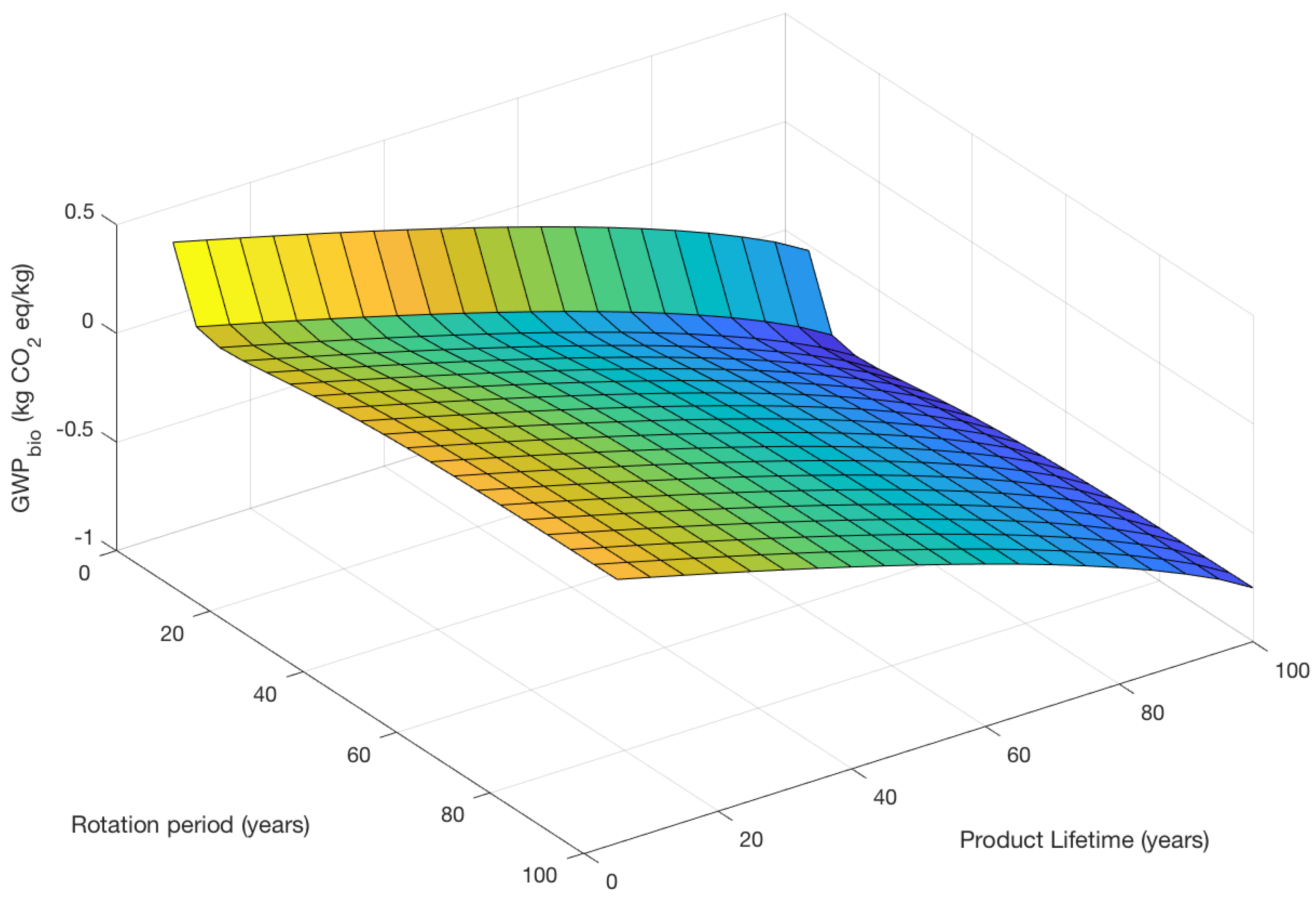
Figure 1 is the central figure of the study and summarizes the main results that have been obtained. It shows a surface plot representation of GWP_bio for 5 kg of cleft timber in terms of its biomass forest rotation period and the product lifetime. The x and y axes represent these two parameters, respectively. The z axis shows the value for GWP_bio, the GWP of the cleft timber’s embodied carbon. This number is taken from the BCFC-HWP and corresponds to the sum of the two following terms: the GWP_{bio, forest}, a term which describes the amount of CO₂ within the different carbon pools of the forest stand as the cleft timber is harvested, and GWP_{bio, storage}, a term for accounting for the storage of CO₂ within the carbon content of the cleft timber HWP. Plotting the sum of GWP_{bio, forest} and GWP_{bio, storage} as a function of biomass forest rotation period and product lifetime results in the surface shown in Figure 1.

This surface plot shows a decreasing trend in GWP_bio with respect to y for all x values. Furthermore, the profile of this decrease in GWP_bio with respect to y seems constant for all x, suggesting it is independent of the x variable. These graphical features indicate that the GWP_bio of the analyzed cleft timber product decreases with respect to the product lifetime, and that the form of this decrease is independent of the rotation period of the biomass raw material used.

Looking now at the evolution of the GWP_bio surface with respect to the x axis, a seemingly constant profile can again be observed for all y. This profile appears as having an initial steep decrease, followed by a more gradual increase. This pattern seems identical for all y, suggesting that it is independent of the y variable. The deductions which can be reasoned from these graphical observations are that, on the one hand, the GWP_bio of the analyzed cleft timber product is neither constantly decreasing nor constantly increasing with respect to the biomass rotation period, and that, on the other hand, the observed decreasing-then-increasing pattern of GWP_bio is independent of the lifetime of the product.

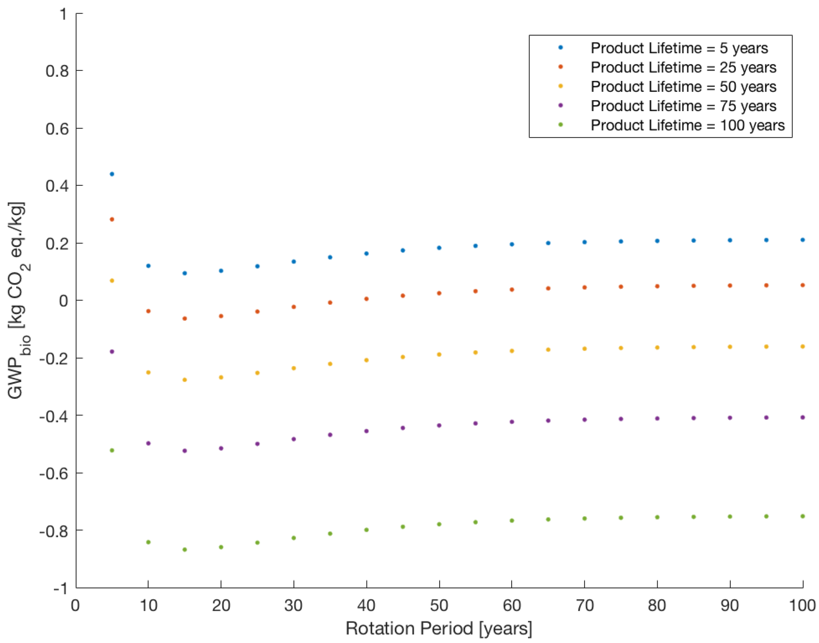
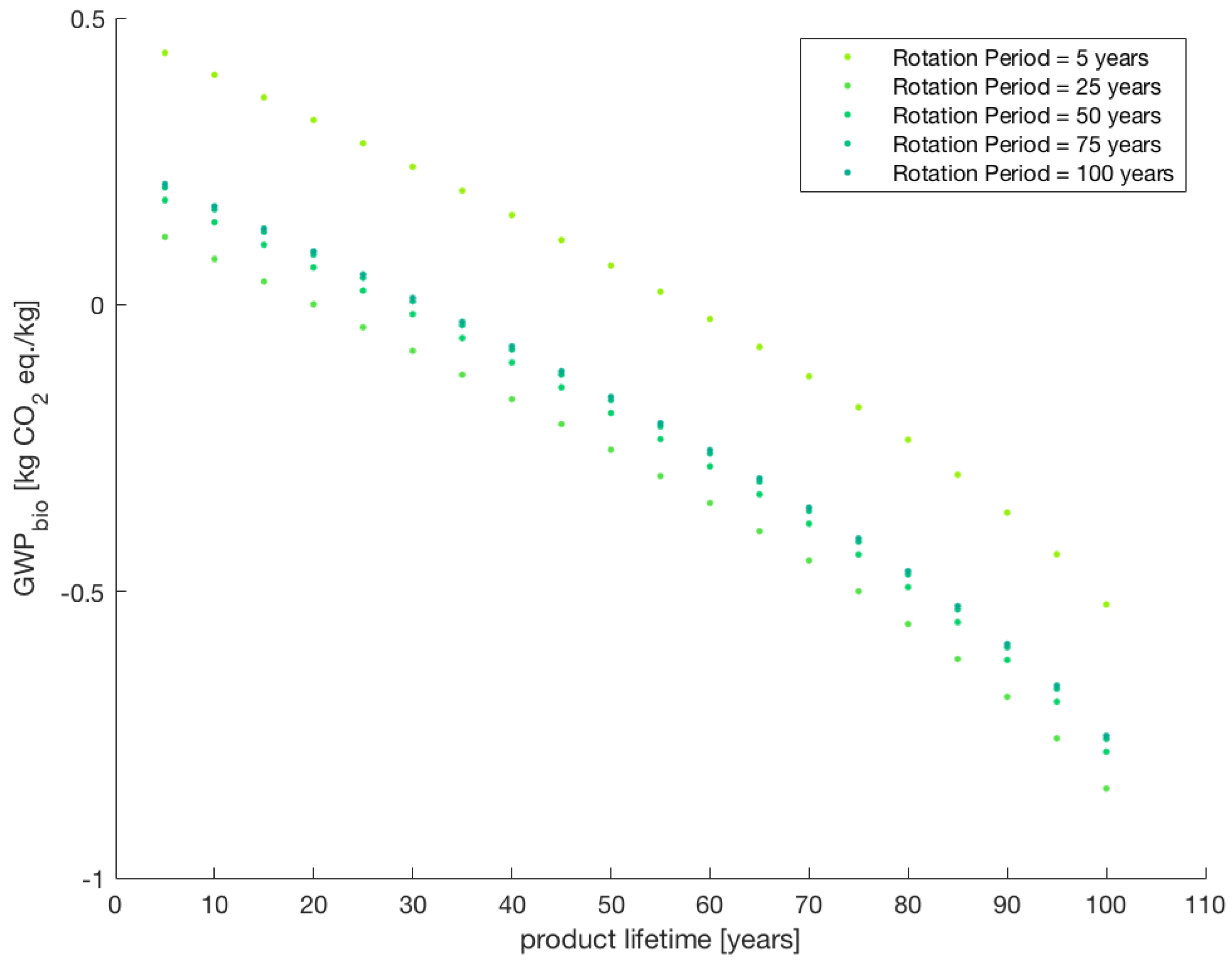
Figure 2 and Figure 3 show similar information to Figure 1, only the plots are organized into overlays. In order not to overcrowd the figure, only certain scenarios were included in either plot. These plots highlight the trends already observed in Figure 1. In Figure 2, the consistency in the profile of GWP_bio vs. the rotation period as the product lifetime increases is seen. In addition, Figure 2 brings to light the fact that the value of GWP_bio itself decreases as the product lifetime is increased: the GWP_bio vs. rotation period curves of a similar profile are successively below each other for increasing product lifetimes. In fact, Figure 2 reveals an additional feature concerning the evolution of the value of GWP_bio with respect to the product lifetime: seen graphically as an increase in the space between the stacked GWP_bio vs. rotation period curves, this feature is due to the fact that GWP_bio not only decreases with respect to the product lifetime, but that this decrease is itself intensified as the product lifetime extends. This last feature can also be observed graphically in Figure 1 through the steeping in the slope of all GWP_bio vs. product lifetime curves.

As for Figure 3, it also echoes the trends that were noted when observing Figure 1. Notably, it shows the constant profile of GWP_bio’s evolution with respect to the product lifetime as the biomass rotation period is modified. These identical profiles, however, have an arrangement which attests for the evolution in GWP_bio with respect to the forest rotation period: the highest curve (shown in blue) corresponds to a short forest rotation period (5 years) while the following curves, which correspond to biomass rotation periods of 25, 50, 75 and 100 years, respectively, are below it but sequentially above one another, suggesting that theses curves have a lower but progressively increasing GWP_bio: this graphical arrangement of curves echoes the fact that GWP_bio is initially high for early rotation periods but then drops and gradually increases.

It is not straightforward to draw conclusions based on the observations made in Figure 1, Figure 2 and Figure 3. The evolution in GWP_bio with respect to product lifetime (clearly visible in each overlay curve in Figure 3) shows a consistent decrease whereas the evolution of GWP_bio with respect to rotation period (the overlays of Figure 2) shows an irregular trend of an initial decrease then increase. Therefore, the relative effect of increasing the product lifetime versus decreasing the biomass rotation period cannot be readily computed and resolutions as to which of the two strategies should be followed cannot reliably be made. On the other hand, if only GWP_bio’s evolution with respect to the product lifetime is considered, one can affirm that, based on this specific case of a 5 kg cleft timber product, increasing the product lifetime is an advantageous strategy that can be followed for improving an HWP’s climate effect.

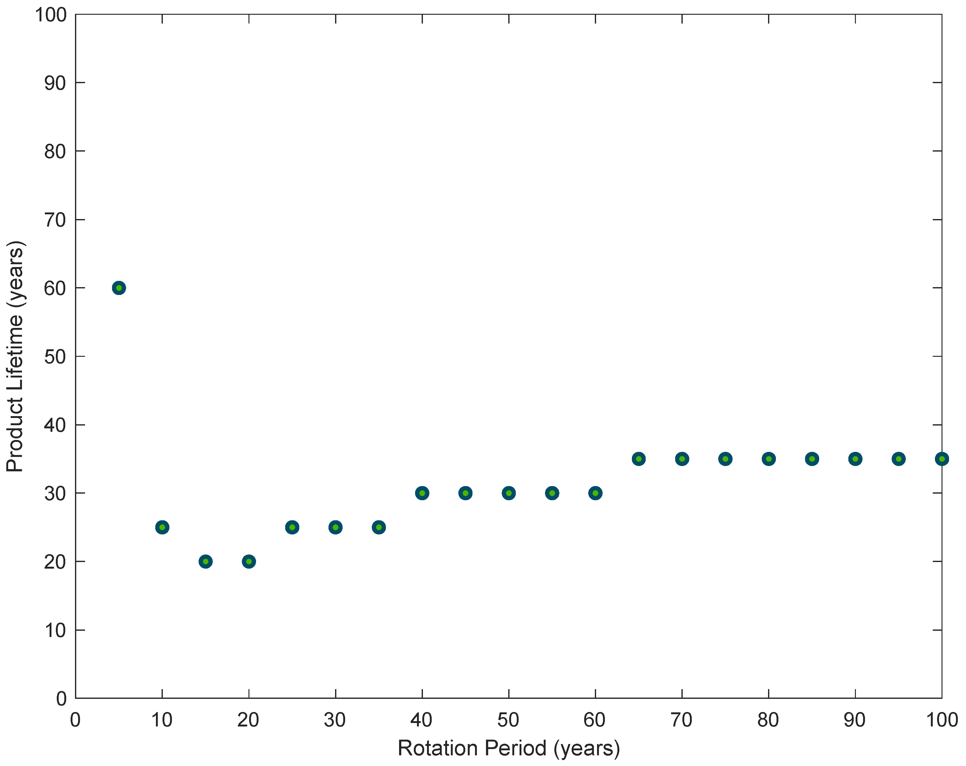
In addition to observing the effects that the biomass forest rotation period and product lifetime have on the potential climate benefits of an HWP, the results obtained through this study also allow for observing the points of climate neutrality. Climate neutrality is reached when the product’s GWP_bio is equal to zero; when the GWP_bio is a positive number, this means the product is contributing positively to the warming of the climate and when its GWP_bio is negative, this, in turn, means that the HWP is contributing negatively to the warming of the planet. In Figure 4, the points at which the cleft timber HWP becomes climate neutral are shown with respect to the forest rotation period of the biomass. This information is plotted as the product lifetime necessary for the cleft timber to show climate neutrality as a function of the biomass rotation period. In reality, since a non-continuous set of GWP_bio values was used, Figure 4 plots the product lifetimes necessary for a first negative GWP_bio: i.e., the first product lifetime at which the product begins to contribute negatively to the warming of the planet.

A similar trend to the one observed in Figure 1 concerning the evolution of GWP_bio with respect to the forest rotation period is observed here. This is expected as the evolution of GWP_bio dictates the storage required for reaching a negative GWP_bio.

4. Conclusions

The present study looked to compare the relative climate benefits associated with two climate mitigation strategies: increasing the storage time of carbon within the anthroposphere, on the one hand, and hastening the time for carbon recapture by biomass on the other. It used a biogenic carbon accounting tool, the BCFC-HWP by Quantis, in order to make observations on the relative importance of these two strategies. An analysis was performed on the two following parameters: the rotation period of the biomass source and the length of the wood product’s lifetime.

The results of the study, however, show the complexity of the two analyzed strategies in mitigating climate change. Nonetheless, lessons could be obtained from the observations made on the evolution of GWP_bio with respect to the product lifetime and the biomass rotation period. The results showed that while GWP_bio followed a consistent decrease with respect to the product lifetime parameter, it showed a non-consistently evolving trend with respect to the biomass rotation period, first decreasing then increasing. The evolution with respect to the product lifetime appeared to be a decreasing one, making the following deduction possible: increasing the lifetime of HWPs is an effective strategy in decreasing the climate warming effect of this HWP. It can thus be concluded that strategies which prolong the material lifetime such as the re-use of products are advantageous resolutions in decreasing the effect which an HWP has on the warming of the planet.