Article

Estimation Method of Short-Circuit Current Contribution of Inverter-Based Resources for Symmetrical Faults

by
Murillo Cobe Vargas
1,*,
Oureste Elias Batista
2 and
Yongheng Yang
3
1
Federal Institute of Espirito Santo, Al. Francisco Vieira Simões, 720, Guarapari 29216-795, Brazil
2
Electrical Engineering Department, Federal University of Espirito Santo, Av. Fernando Ferrari 514, Vitoria 29075-910, Brazil
3
College of Electrical Engineering, Zhejiang University, Zheda Rd. 38, Xihu, Hangzhou 310027, China
*
Author to whom correspondence should be addressed.
Energies 2023, 16(7), 3130; https://doi.org/10.3390/en16073130
Submission received: 19 February 2023 / Revised: 13 March 2023 / Accepted: 24 March 2023 / Published: 30 March 2023
(This article belongs to the Topic Power System Protection)

Abstract

:
This paper proposes a practical approach to estimate the symmetrical short-circuit current (SCC) levels in overcurrent protection devices (OCPDs) installed on radial feeders for any penetration level of inverter-based distributed energy resources (DERs). The proposed method restores the lost phase protection coordination by estimating SCC values and changing the TMS of OCPDs accordingly. The method is validated by comparing the results with simulations on the IEEE 34-Node Test Feeder using MATLAB/Simulink, which shows an average error of 1.5% and a maximum error of 3.0%. For a 100% penetration level, the SCC variation through OCPDs installed on the main fault trunk (MFT) exceeds ± 10%, leading to compromised phase protection coordination. The SCC flowing reversely through OCPDs on lateral branches and the fault on the MFT could cause improper tripping. Higher SCC levels are estimated and measured for fault impedances equal to zero. The phase protection is restored by changing the TMS of OCPDs using the estimated values. The study proposes two phase protection schemes to accommodate inverter-based DERs injecting 1.2 pu and 2.0 pu of SCC for a 100% penetration level. This study contributes to improving the protection coordination of distribution networks with high penetration levels of DERs. The findings have practical implications for distribution system operators and planners to maintain safe and reliable operation of distribution feeders.

1. Introduction

Electric power systems are facing challenges with the fast installations of distributed energy resources (DERs) [1]. In this scenario, electronically-coupled resources, such as inverter-based resources (IBRs), are rapidly increasing power and quantity. Despite the small power capacities and SCC contribution from IBRs, their contribution could significantly change the SCC level of the feeeder [2], affecting the traditional distribution system’s protection scheme [2,3,4].
The behavior of IBRs is quite different from the rotating machines during faults [5]. Their SCC contribution is limited by an internal logic control due to the low thermal withstanding capability of the employed semiconductors and components. The SCC contribution could be 1.06–1.2 pu on IBR’s base rating, according to the “rule of thumb” and experimental tests [3,6,7,8], or 1.1–1.5 pu [9,10]. Moreover, this SCC envelope decay is fast and is divided in two parts: the first one with an initial spike with only a few hundred microseconds or less, in which the current may be higher than 2.0 pu on the IBR’s base rating; the second with a regulation period of a few hundred milliseconds, varying from the technology and control embedded by the manufacturer [11]. Furthermore, IBRs are grid-following, not controlled by the distribution grid operator (DNO) or consumer unit and are usually associated with a variable source of renewable energy, e.g., photovoltaics (PV) and wind power. Therefore, IBRs present several challenges to predict their behavior correctly [12].
Additionally, updated grid codes, e.g., the IEEE 1547-2018 [13], require the DERs to withstand voltage and frequency variations exchanging active and/or reactive power with the grid, and that they have different operation modes such as: Volt-Watt, Volt-VAR, Watt/VAR, constant power factor and constant reactive power. Those requirements aim to help the post-fault grid recovery to avoid severe power outages. However, they become a challenge for the feeder protection coordination [14].
Accordingly, the fault characteristics of the IBRs combined with their aggregated SCC contribution, could affect the power system in different ways as follows [3,9,12,15,16,17,18,19,20,21]:
  • The change in the fault current level, whose value is applied to adjust the coordination time interval (CTI) between adjacent overcurrent protection devices (OCPDs);
  • The coordination loss, highlighting the blind protection, sympathetic tripping and fuse protection philosophy (fuse-blow and fuse-saving);
  • The change in the load current, whose value is used to adjust the sensitivity of the OCPDs.
Furthermore, if the SCC contribution from energy sources is not correctly predicted and considered during studies of power system protection, network planning, maintenance and operation, then the distribution network (DN) and its stakeholders may face a decrease in financial income, reliability, resiliency and robustness, as well as an increase in maintenance costs, time and frequency interruption [22]. In this context, one of the main challenges is to estimate or compute the SCC contribution by each IBRs dispersed in the DN, within a variety of possible DER integration scenarios, and how this affects the DN protection coordination [9].
Estimation of the SCC contribution can be approached by mathematical equations, computer simulations or through laboratory experiments that test commercial smart inverters under faulty scenarios. As the IBRs limit its output current by internal controllers, the inverter should be modeled as an internally limited or unlimited current source for an SCC analysis [22]. Thus, it should be considered a current source inverter (CSI) [23,24,25].
Transient IBR models incorporate complicated methods to calculate the SCC contribution, as the d-q axis, in addition to being modeled at the dynamic level, which require many variables and small time steps, making the simulations time- and computational consuming [26]. Moreover, the efforts for implementing simulations of large feeders with many dispersed IBRs are significant. This approach may not be necessary for a steady-state SCC contribution calculation.
The estimation of the SCC contribution has been proposed and studied in other transient and steady-state SCC papers. In [2], the output current of a small-scale PV generator, modeled using Simulink in MATLAB, was limited up to 2.0 pu. The SCC contribution magnitude through OCPDs was considered relevant and capable to affect the coordination and selectivity of the power system protection. The work of [4] analyzes recorded fault events, showing that the SCC contribution in steady-state was less than the rated output current. On the other hand, a considerable reduction in fault currents seen by the upstream relay was noticed, making it necessary to review the relay settings. In [7], a series of experimental tests was done with commercial inverters. The results reported by the authors showed an insignificant or minimal SCC contribution of IBRs for low penetration levels of DERs. However, that effect may become invalid in high penetration scenarios. In [27], a practical methodology to analyze the SCC contribution of various DETs during shunt faults, has been proposed for use in advanced distribution management systems. These previous studies highlight that an inaccurate modeling of the IBR or its consideration for an SCC analysis could compromise the reliable and safe DER integration in DN and power systems.
A series of SCC calculations in steady-state, using current injection matrices, for balanced and unbalanced situations with the presence of IBRs, was proposed by I. Kim [22,28,29]. New equations were derived to estimate the SCC flowing from IBRs. However, the impacts on the protection coordination of a power system were not presented and discussed.
In previous works [30,31], an accurate power flow calculation method for active networks in sequence-domain considered two SCC contribution control strategies from IBRs, compared with other existing methods that do not fit these source elements. The method proposed in [31] calculates the SCC contribution for any SCC conditions, without predefined boundary conditions. The SCC contribution of the IBRs is calculated depending on the pre-fault current condition and voltage at the node where the IBR is connected. Using this method, a novel relay protection coordination was proposed by [32], which considers the DER disconnection for fault ride-through and the relay operating times need to be recalculated every time the DER is disconnected from the network.
Finally, the work of L.G.R. Tonini et al. [33] from the authors’ research group, proposes a load flow and SCC method based on the backward/forward sweep method and hybrid impedance matrix, respectively, considering the operating modes of IBRs, based on IEEE 1547–2018, and considering each of the renewable sources as a voltage-controlled current source. Once more, modifications to the system protection based on the found values were not proposed.
Therefore, the motivation of this paper was the lack of studies to reconfigure the DN protection coordination with a single adjustment considering the change in SCC level of the DN with the massive presence of IBRs, as well as the lack of SCC calculation methods that are easier to understand and apply, especially for industry professionals who are not up to date or not very familiar with the complex mathematics of power flow and short circuit calculation methods. Current methods, as presented previously, take into account many IBR control variables that may not be necessary to estimate the feeder SCC level from the overcurrent protection perspective.
In light of the above, this paper proposes a simple and practical approach to estimate the steady-state SCC contribution in a balanced DN, dominated by IBRs during symmetrical faults. This approach is not intended to be extremely accurate, but to return an approximate value for evaluating the feeder when it has high DER penetration. The approach considers the IBR as a limited current source and its relative electrical distance on the feeder in relation to OCPD and substation. The study also proposes a phase protection coordination methodology, which uses the estimated SCC in extreme situations, to ensure the feeder protection coordination for a wide penetration range of IBRs, without or with the minimum need to replace the installed OCPDs.
In other words, a simple and practical method that can be applied on a daily basis to verify whether the SCC level of a given feeder, which can be dominated by IBRs, can reach critical values. In the affirmative case, we propose a single adjustment to the feeder protection coordination to accommodate these new inverter-based DERs. The assertiveness and effectiveness of the approaches were validated through MATLAB/Simulink simulations.
The remainder of the paper is organized as follows. In Section 2, the proposed approach to estimate the SCC contribution is presented, and the sensitivity analysis of the equations is made in Section 3. A protection coordination scheme for IBR-dominated power systems is presented in Section 4. A case study on the IEEE 34-Node Test Feeder is performed in Section 5 with the application of the approach to estimate the SCC, the impacts on SCC level and protection coordination, as well as the change in the OCPDs settings, followed by a discussion of the applications. Conclusions are drawn in Section 6.

2. Estimating the Short-Circuit Current Contribution for Symmetrical Faults

Currently, distribution feeders are being dominated by IBRs that can be installed along it at many different locations with different power ratings, and consequently, affecting the fault current level through the installed OCPDs. Accordingly, an analysis must be performed for situations with high integration and high penetration level (PL) of IBRs, i.e., several IBRs installed at different locations.

2.1. Distribution Feeder without Lateral Branches

Figure 1 shows a radial distribution feeder, without lateral branches, dominated by IBRs installed on the main fault trunk (MFT) of the feeder. The distribution feeder has balanced impedances and no loads connected, while a purely faulty network is considered.
For a three-phase line-to-ground (3LG) fault at point F, downstream from all protection devices, without the IBRs, the currents per phase through OCPD1 and OCPD2 are given by Equation (1) [34].
i o c p d 1 = i o c p d 2 = i f = v s z t + z l i n e + z f = v s z l f
where i f is the fault current contribution from the substation, i o c p d 1 and i o c p d 2 are the fault currents through OCPD1 and OCPD2, respectively, v s is the pre-fault voltage at substation, z t is the substation transformer short-circuit impedance, z l i n e is the total impedance of the line between the substation and the fault point, z f is the fault impedance, and z l f is the sum of z t , z l i n e and z f . All variables are given in the per unit (pu) system.
When the IBRs are located only downstream from OCPD1 and OCPD2 (IBRk, IBR(k+1), …, IBRm, from Figure 1), considering the same 3LG fault discussed previously, the currents through the OCPDs are the same and given by Equation (2).
i o c p d 1 = i o c p d 2 = 1 z l f v s + k = 1 m i i b r k ( z i b r k + z t z l f )
where i i b r k is the output current of the kth IBR located downstream from the protection devices, z i b r k is the electrical distance between the kth IBR and the substation, and m is the total of IBRs installed between OCPD2 and the fault point F.
When the IBRs are located only upstream from OCPD1 (IBRj, IBR(j+1), …, IBRw, from Figure 1), taking into consideration the previous fault condition, the currents through OCPD1 and OCPD2 are the same as presented in Equation (3).
i o c p d 1 = i o c p d 2 = 1 z l f v s + j = 1 w i i b r j ( z i b r j + z t )
where i i b r j is the output current of the jth IBR located upstream from OCPD1, z i b r j is the impedance between the jth IBR and the substation, and w is the total of the IBRs installed upstream from OCPD1.
Finally, when the IBRs are located only between OCPD1 and OCPD2 (IBRi, IBR(i+1), …, IBRn, from Figure 1), the currents through OCPD1 and OCPD2 are different and given by Equations (4) and (5), respectively.
i o c p d 1 = 1 z l f v s + i = 1 n i i b r i ( z i b r i + z t z l f )
i o c p d 2 = 1 z l f v s + i = 1 n i i b r i ( z i b r i + z t )
where i i b r i is the output current of the ith IBR located between the protection devices, z i b r i is the impedance between the ith IBR and the substation, and n is the total of the IBRs installed between OCPD1 and OCPD2.

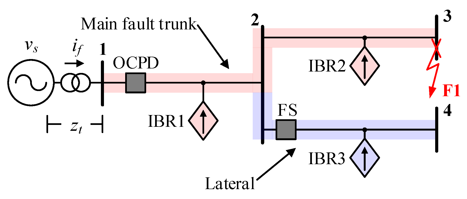
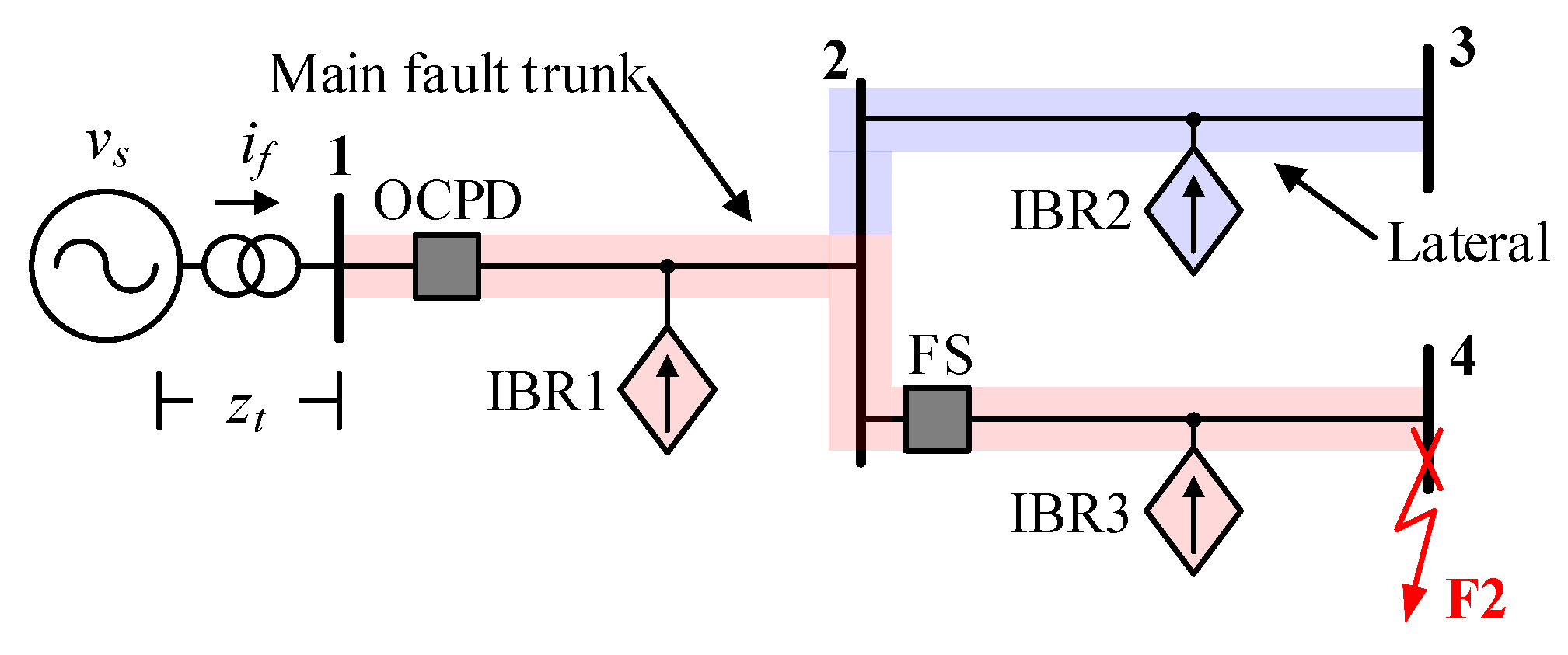
2.2. Distribution Feeder with Lateral Branches

A real radial distribution feeder has several lateral branches, with IBRs installed, and these laterals are mostly protected by fuses. Figure 2 and Figure 3 show a simple radial distribution feeder with three IBRs and two branches: 2–3 and 2–4. Branch 2–4 is protected by a fuse (FS). The feeder has balanced impedances and no loads connected.

2.2.1. Fault without IBRs

Considering the Figure 2 and Figure 3, for a 3LG fault at point F1 and F2, without the connection of IBRs, the currents through the OCPD ( i o c p d ) and the fuse ( i f u s e ) are given by Equations (6) and (7) for Figure 2 and Equation (8) for Figure 3, where z 12 , z 23 , and z 24 represent the impedance between buses 1–2, 2–3 and 2–4, respectively, and z f the fault impedance, also in pu.
i f u s e = 0
i o c p d = v s z t + z 12 + z 23 + z f
i o c p d = i f u s e = v s z t + z 12 + z 24 + z f

2.2.2. Fault with IBRs

Taken Figure 2 into consideration, the MFT comprehends branches 1–2–3 and the lateral branch 2–4. Considering the connection of IBR1 and IBR2, only, the currents through the devices are given by
i f u s e = 0
i o c p d = 1 z l f 13 [ v s + i i b r 1 ( z i b r 1 + z t z l f 13 ) + i i b r 2 ( z i b r 2 + z t z l f 13 ) ]
where z l f 13 = z t + z 12 + z 23 + z f . This case represents the situation where the fault occurs on the MFT and the IBRs are installed on it.
When only IBR3 is connected, the currents through the devices are different. In this case, IBR3 will contribute with an SCC to the fault point F1, and a reverse fault current will flow through the fuse. Therefore, the currents through the devices can be given by
i f u s e = i i b r 3
i o c p d = 1 z l f 13 [ v s + i i b r 3 ( z 12 + z t z l f 13 ) ]
where z 12 is the electrical distance of the lateral 2–4 to the substation. The location of the IBR in the lateral, i.e., beginning or end, does not influence the current through the upstream OCPD and the fuse.
Now, taking Figure 3 into consideration, the MFT comprehends the branches 1–2–4, and the lateral branch 2–3. Considering the connection of IBR1 and IBR3, the currents through the devices are given by
i o c p d = 1 z l f 124 [ v s + i i b r 1 ( z i b r 1 + z t z l f 124 ) + i i b r 3 ( z i b r 3 + z t z l f 124 ) ]
i f u s e = 1 z l f 14 [ v s + i i b r 1 ( z i b r 1 + z t ) + i i b r 3 ( z i b r 3 + z t z l f 14 ) ]
where z l f 14 = z t + z 12 + z 24 + z f . This case represents the situation where the fault occurs on the MFT and the IBRs are installed on it.
When only IBR2 is connected, the currents through the devices are different and can be given by
i o c p d = 1 z l f 124 [ v s + i i b r 2 ( z 12 + z t z l f 124 ) ]
i f u s e = 1 z l f 124 [ v s + i i b r 2 ( z 12 + z t ) ]
where z 12 is the electrical distance of the lateral branch to the substation. In this case, IBR2 will contribute with an SCC to the fault point F2, injecting its current through the point of connection of the lateral. As discussed, and according to Equation (12), the location of the IBR in the lateral branch does not influence the current through the upstream OCPD and the downstream fuse.

2.2.3. Feeder Dominated by IBRs

In the case of Equations (12), (15) and (16), the position of the IBR on the lateral branch does not influence on the current through the upstream and downstream OCPDs. Thus, the electrical distance from the point of interconnection of the lateral branch with the MFT is the variable of interest.
For a radial distribution feeder with lateral branches and IBRs installed only on them, the current through any OCPD can be given by
i o c p d = 1 z l f v s Substation + i = 1 n i i b r i ( z b r a n c h i + z t ) Upstream   lateral   with   IBRs + 1 z l f k = 1 m i i b r k ( z b r a n c h k + z t z l f ) Downstream   lateral   with   IBRs
where z l f is the sum of z t , z f and the impedance between the substation and the fault point, and z b r a n c h i and z b r a n c h k are the electrical distance of the ith and kth branch from the substation upstream or downstream from the OCPD, respectively.
The general equation that describes when the IBRS are connected on a lateral branch, downstream of the OCPD that protects that side, and there is a 3LG fault on the MFT, is given by:
i o c p d = i = 1 n i i b r i
where the negative signal means the reverse current flows through the device, i.e., the SCC contribution flows from the lateral branch to the MFT.

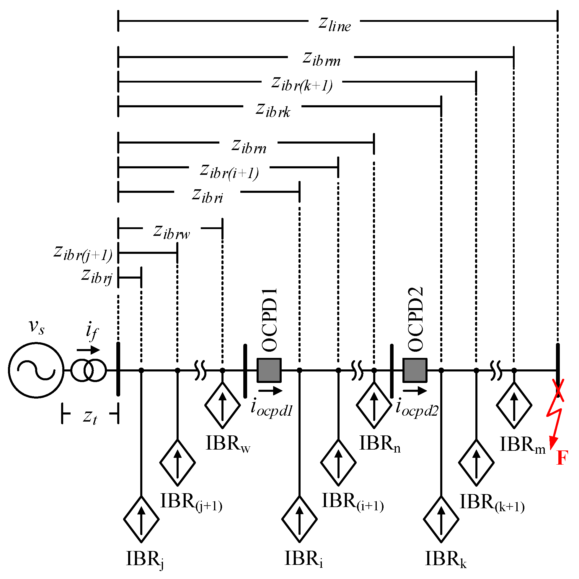
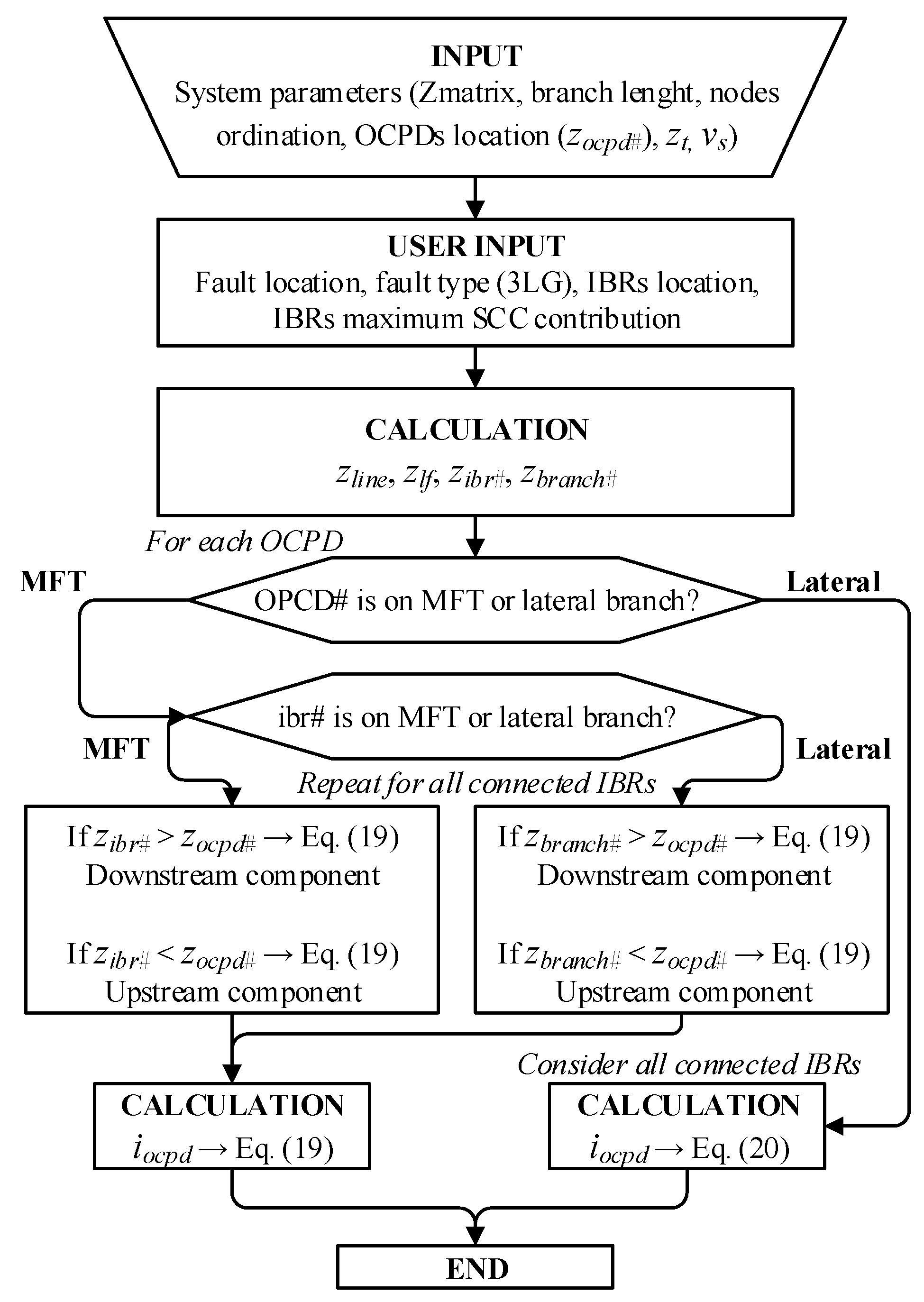
2.3. A General Equation

The 3LG fault current through any OCPD in any distribution feeder with the integration of IBRs can be determined by the relation between the SCC contribution from three different sources:
  • The substation;
  • The IBRs located upstream seen from the perspective of the OCPD;
  • The IBRs located downstream seen from the perspective of the OCPD.
The fault current through any OCPD installed on the MFT can be given by Equation (19), where z l f is the sum of z t , z f and the impedance between the substation and the fault point. For IBRs installed upstream from the OCPD, the current through it increases its value. On the other hand, when the IBRs are installed downstream from the OCPD, the current decreases.
When the OCPD is installed on a lateral branch with IBRs installed downstream of the OCPD and the fault occurs on the MFT, the current through this OCPD is given by Equation (20), where the negative signal means the reverse flow of the current through it. The block-diagram of the proposed SCC calculation is presented in Figure 4.
i = 1 z l f [ v s + i = 1 n i i b r i ( z i b r i + z t ) + k = 1 r i i b r k ( z b r a n c h k + z t ) Upstream   IBRs - increase   fault   current + l = 1 p i i b r l ( z i b r l + z t z l f ) + m = 1 q i i b r m ( z b r a n c h m + z t z l f ) Downstream   IBRs - decrease   fault   current ]
i = u = 1 t i i b r u

3. Sensitivity Analysis of the General Equations

It is important to understand the behavior and know the extreme fault current cases in which the OCPDs are subjected to under scenarios of a high integration of IBRs. Under those extreme scenarios, it is possible to highlight the maximum and minimum currents through an OCPD for each fault type.
As shown in Figure 5, for example, each OCPD can experience a wide variation of fault currents and tripping times due to the presence of the IBRs. These extreme situations can be provided to DNOs, which is important to verify the robustness and reliability of the current protection scheme for a scenario of a high PL of DERs.
When there are no IBRs connected to the grid, the coordination time interval (CTI) between two OCPDs can be determined using the classic method because, in this situation, i o c p d 1 = i o c p d 2 for a pure fault circuit. However, when IBRs are connected to any point of the feeder, the current through OCPD1 and OCPD2 can be at its maximum ( i o c p d 1 m a x and i o c p d 2 m a x ) or minimum ( i o c p d 1 m i n and i o c p d 2 m i n ).
Therefore, it is essential to analyze the sensitivity of the variables in Equations (19) and (20) concerning the maximum and minimum fault currents through the OCPDs. In other words, it is necessary to identify which cases and variables of interest determine the maximum or minimum current through the OCPDs.

3.1. OCPD Installed on Main Fault Trunk

As discussed previously, the fault current through an OCPD in the presence of an IBR is influenced by three components. Therefore, an analysis will be carried out considering only upstream IBRs and, subsequently, only downstream IBRs.

3.1.1. Upstream IBRs

When there are only IBRs installed upstream from the OCPD, Equation (19) can be rewritten as Equation (21) for a 3LG fault.
i o c p d = v s z l f I + i = 1 n i i b r i ( z i b r i + z t ) z l f II + k = 1 r i i b r k ( z b r a n c h k + z t ) z l f III
Component I represents the substation contribution, which is the main source of the short-circuit capacity. The fault current value depends on z l f , which is composed of the impedance components of the substation power transformer, the line, and the fault impedance. Component II represents the IBRs installed in the MFT. By analyzing this component independently, the value of i i b r i during a severe fault may be considered constant, within the range of 1.06 to 1.20 pu (as stated in Section 1), and also the value of z t and z l f , independent of the IBR location. Thus, the value that can be changed is the electrical distance of the IBR, z i b r i . In terms of the distance of the IBR from the OCPD, it can only be less than or equal to the electrical distance of the OCPD from the substation ( z o c p d ) to guarantee that the IBRs are upstream from the OCPD. Thus, the value of component II will be maximum when z i b r i = z o c p d because it is the maximum electrical distance at which the IBR can be installed to be upstream from the OCPD. Making a similar analysis for component III, its value will be maximum when z b r a n c h k = z o c p d .
Accordingly, the maximum fault current through an OCPD will occur when the power of the IBRs, and consequently, the SCC injection, is installed right before the OCPD, either in the MFT or in a lateral.

3.1.2. Downstream IBRs

When there are only IBRs installed downstream from the OCPD, Equation (19) can be rewritten as Equation (22) for a 3LG fault.
i o c p d = v s z l f I + i = 1 n i i b r i ( z i b r i + z t z l f ) z l f II + k = 1 r i i b r k ( z b r a n c h k + z t z l f ) z l f III
Component I is the same as discussed in the previous subsection. Component II represents the IBRs installed in the MFT. Making an independent analysis of this component, the value of i i b r i during a severe fault may be considered constant, within 1.06–1.20 pu, as stated in Section 1, and the values of z t and z l f are also constant. Therefore, the only variable that can be changed is the electrical distance of the IBR, z i b r i . In terms of the distance of the IBR from the OCPD, it can only be equal to or greater than z o c p d , ensuring that IBRs are downstream from the OCPD. Thus, the value of component II will be maximum when z i b r i = z o c p d because it is the minimum electrical distance that the IBR can be installed to be downstream from the OCPD. Similarly, for component III, its value will be maximum when z b r a n c h k = z o c p d .
Therefore, the minimum fault current through an OCPD will occur when the sum of the power of the IBRs, and consequently, the SCC injection, is installed right after the OCPD, either in the MFT or in a lateral.

3.2. OCPD Installed on a Lateral of the Main Fault Trunk

In this case, the current through the OCPD will flow in reverse when there are IBRs installed downstream from the OCPD, as previously presented in Equation (20).

3.3. Intermediate Remarks

If the OCPD is a non-directional element, such as a fuse or a relay, it may trip improperly. Therefore, it is necessary to analyze coordination cases between fuses and relays, because:
  • The OCPD may be affected by the minimum fault at the end of the lateral;
  • The reverse fault current through the OCPD may be greater than in the case without IBRs;
  • The load current can be greater than in the case without IBRs.
Therefore, it is important to carry out an analysis of the impacts of this variation on the short-circuit level on the distribution system protection.
Using Equations (19) and (20), it is possible to estimate the penetration scenarios of IBRs in terms of the SCC injected by the generators. The IBRs can be positioned anywhere on the feeder. The worst-case scenarios can be estimated by aggregating the total power of the IBRs right before and after the OCPD for downstream or upstream faults. With these estimated values, changes in the classical OCPD coordination can be made to accommodate the IBRs for any penetration level.

4. Protection Coordination in Distribution Networks Dominated by IBRs

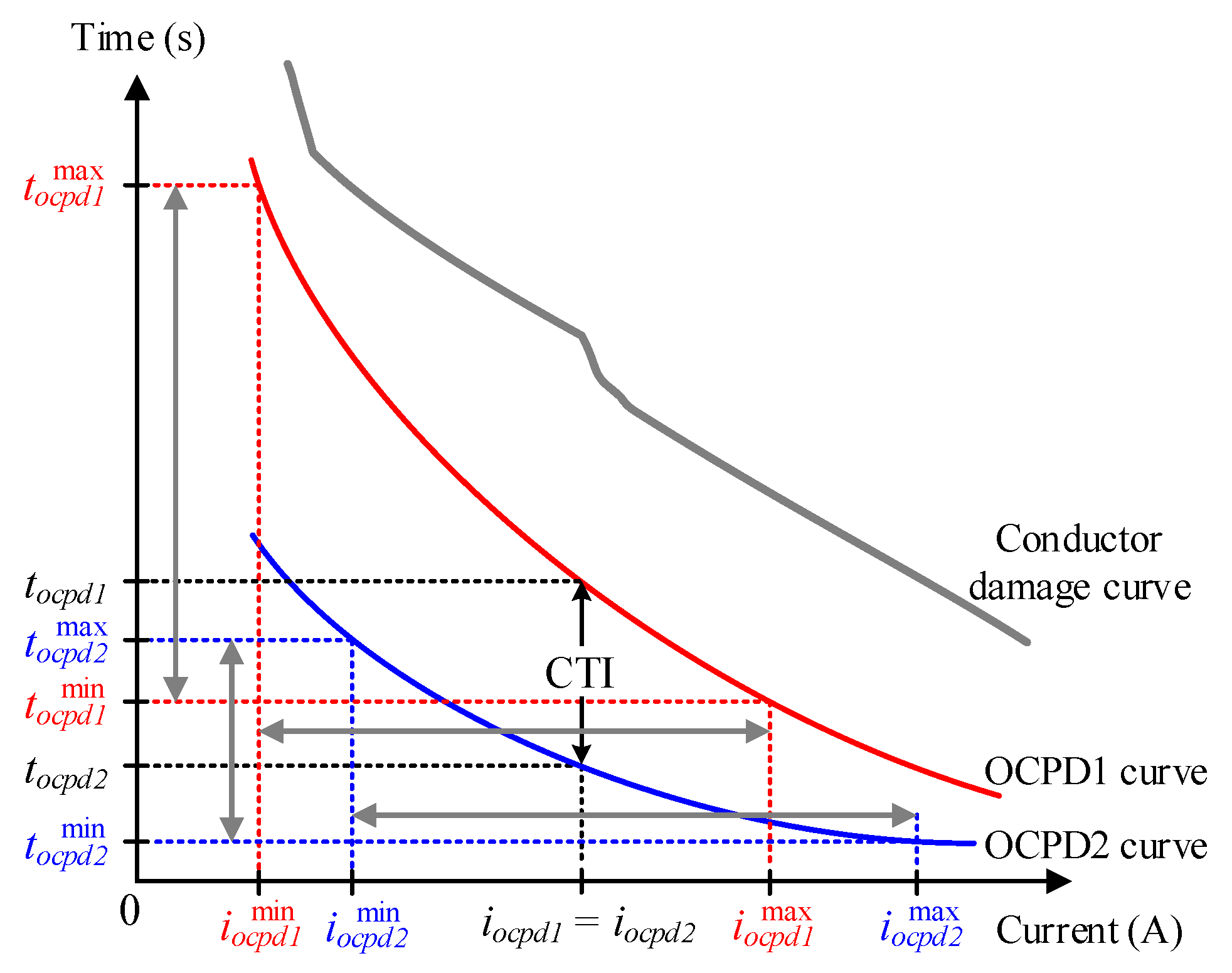
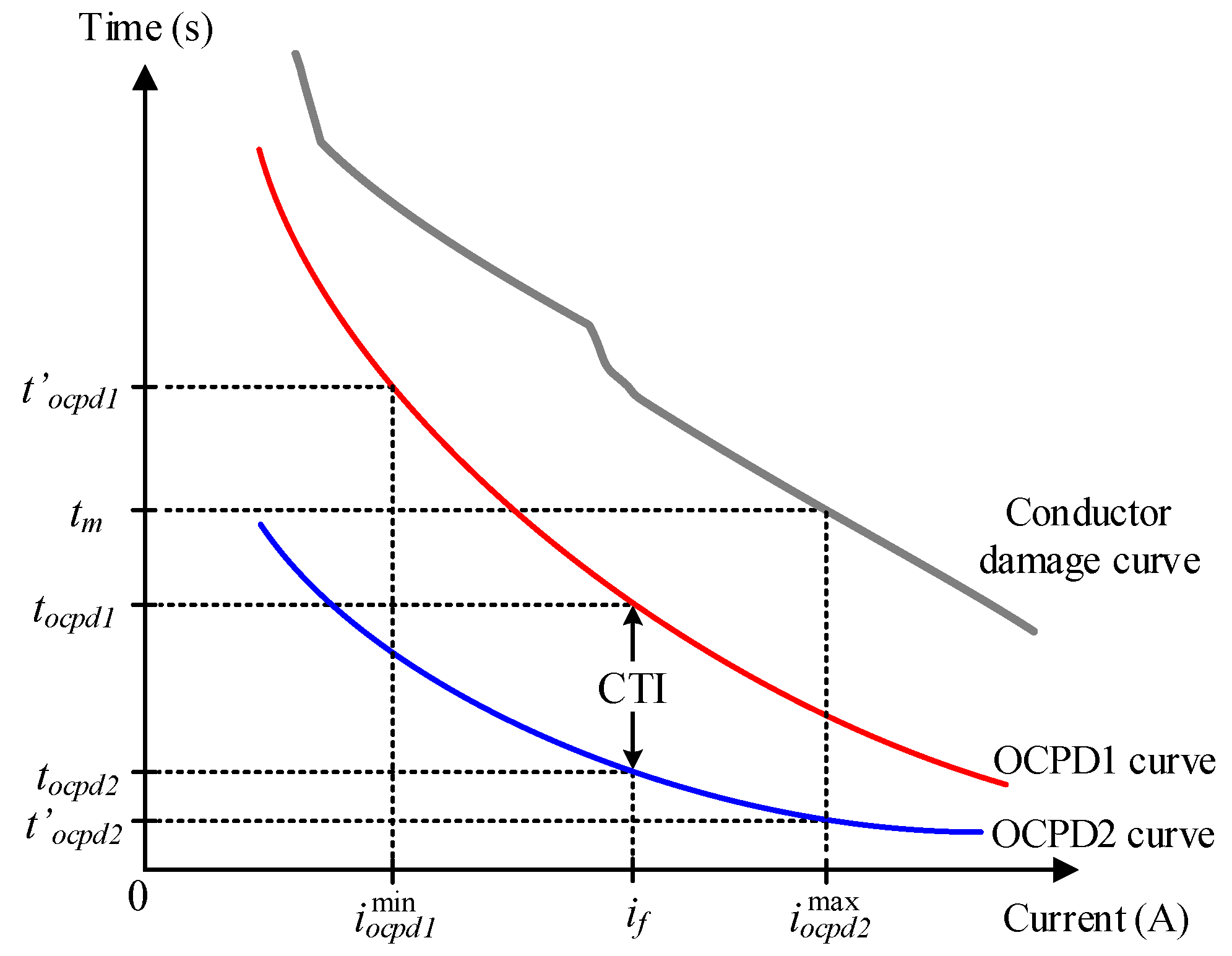
4.1. Classical Protection Coordination

To restore protection coordination between the curves when the conductor’s melting time ( t m ) is not exceeded, and the IBRs are located between the OCPDs, the classical protection coordination scheme can be used [35,36,37,38].
The maximum 3LG fault at the main relay, which is also detected by the backup relay, is used to coordinate the two OCPDs. This maximum fault occurs when the IBRs are upstream from both OCPDs, just before the backup relay or substation relay, as discussed in Section 3. In Section 5, we demonstrate how this value is determined using Equation (19) by considering the extreme scenarios for a high PL of IBRs.

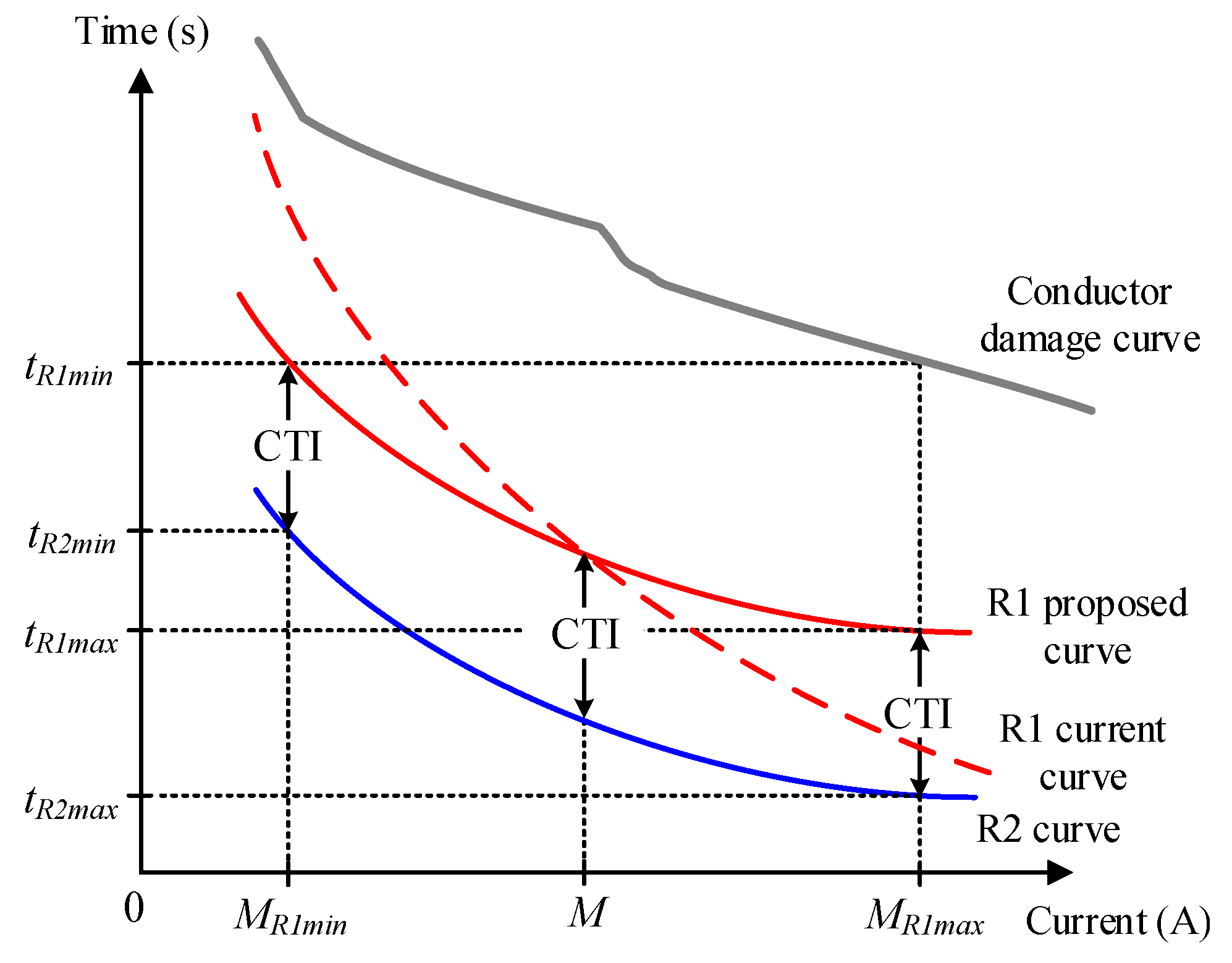
4.2. Changing the Slope of the Characteristic Curves

When the IBRs are connected between the OCPDs, as shown in Figure 1, the operation time of OCPD1 is delayed, and that of OCPD2 is faster than when there are no IBRs. Although this setup appears to improve protection coordination, for a certain SCC injected by the IBRs, the operation time of OCPD1 may exceed the allowable limit for the conductor damage curve, t m , thus disrupting the protection system operation. According to Equation (19), the current through OCPD1 decreases and that through OCPD2 increases when the PL of the IBRs increases. For the maximum SCC contribution from the IBRs, the current through OCPD1 is at a minimum ( i o c p d 1 m i n ), and that through OCPD2 is at a maximum ( i o c p d 2 m a x ), causing them to operate at t o c p d 1 and t o c p d 2 , respectively, as illustrated in Figure 6.
At i o c p d 2 m a x , the maximum fault clearing time must be smaller than t m to protect the feeder’s conductors. If OCPD2 fails to operate at t o c p d 2 , then OCPD1 will only operate at t o c p d 1 , which is greater than t m . Thus, the characteristic curves of OCPD1 and OCPD2 need to be adjusted so that the maximum operation time for the backup relay is less than t m for i o c p d 1 m i n and for coordinating a proper CTI with the downstream relay, ensuring the protection coordination with the integration of IBRs.
Therefore, the slopes of the OCPDs’ curves must be changed. The approach proposed by Fani et al. [39] is presented with adaptations.
With the SCC contribution from the IBRs, the settings of the relays and reclosers must be adjusted for this new scenario. According to IEC [40], the overcurrent relay curve can be obtained using Equation (23).
t = T M S A M P 1
where TMS stands for Time Multiplies Settings, and M is the ratio I m e a s u r e d / I p i c k u p .
The value of the TMS is associated with the coordination–time dial, and the value of M depends on the TMS. The dependency of TMS and the pickup current is that they both affect the tripping characteristics of the OCPD. Increasing the TMS will increase the time delay before the OCPD trips, which can help prevent nuisance tripping but may also delay the tripping response in the event of a fault. Similarly, decreasing the TMS will reduce the time delay before the OCPD trips, which can improve the response time but may also increase the risk of nuisance tripping. Considering that TMS and M are constant, the parameters A and P can be used to change the curve characteristics. Therefore, it is possible to coordinate the backup relay with the main relay of a distribution feeder dominated by IBRs.
In the absence of IBRs, the coordination curves between two relays, backup (R1) and main (R2), are presented in Figure 7 by the current curve R1 (dashed in red) and the curve R2 (in blue), respectively. Under this scenario, the fault currents through the devices are identical, represented as M, with a proper CTI.
However, in the presence of IBRs, the current through the OCPDs may change in a range of maximum and minimum currents, depending on the IBRs’ location and power rating. In these extreme scenarios, the CTI between the OCPDs can assume values below the recommended limit, and tripping times beyond the conductor damage curve. Therefore, the backup relay curve needs to be adjusted, as shown in Figure 7, to be the proposed curve R1, guaranteeing that the two restrictions are fulfilled.
To determine the new parameters for the proposed curve, a suitable CTI must be introduced between the tripping times of the relays for the maximum and minimum values of M. Thus, for t R 1 m i n and t R 1 m a x , as per Equation (23):
t R 1 m i n = T M S A M R 1 m i n P 1
t R 1 m a x = T M S A M R 1 m a x P 1
Rearranging the equations, gives
A · T M S = t R 1 m i n ( M R 1 m i n P 1 )
A · T M S = t R 1 m a x ( M R 1 m a x P 1 )
To ensure the minimum CTI between R1 and R2, a proper CTI is added between the tripping times of the relays as
t R 1 m a x = t R 2 m a x + C T I
t R 1 m i n = t R 2 m i n + C T I
where the value of t R 1 m i n must be less than the melting time of the conductor ( t m ) for the M R 1 m a x and less than the maximum operation time of the distribution substation relay, whichever is less.
The new value of P can be calculated following
t R 1 m i n · M R 1 m i n P t R 1 m a x · M R 1 m a x P + ( t R 1 m a x t R 1 m i n ) = 0
Therefore, the value of A can be found as
A = t R 1 m i n T M S ( M R 1 m i n P 1 )
A = t R 1 m a x T M S ( M R 1 m a x P 1 )
The values of M R 1 m i n and M R 1 m a x are given by Equations (19) or (20), considering the extreme scenarios for a high PL of IBRs, to be determined. This method may be more suitable for main and backup relays with different inverse-time characteristic curves, when it is necessary to change the slopes.

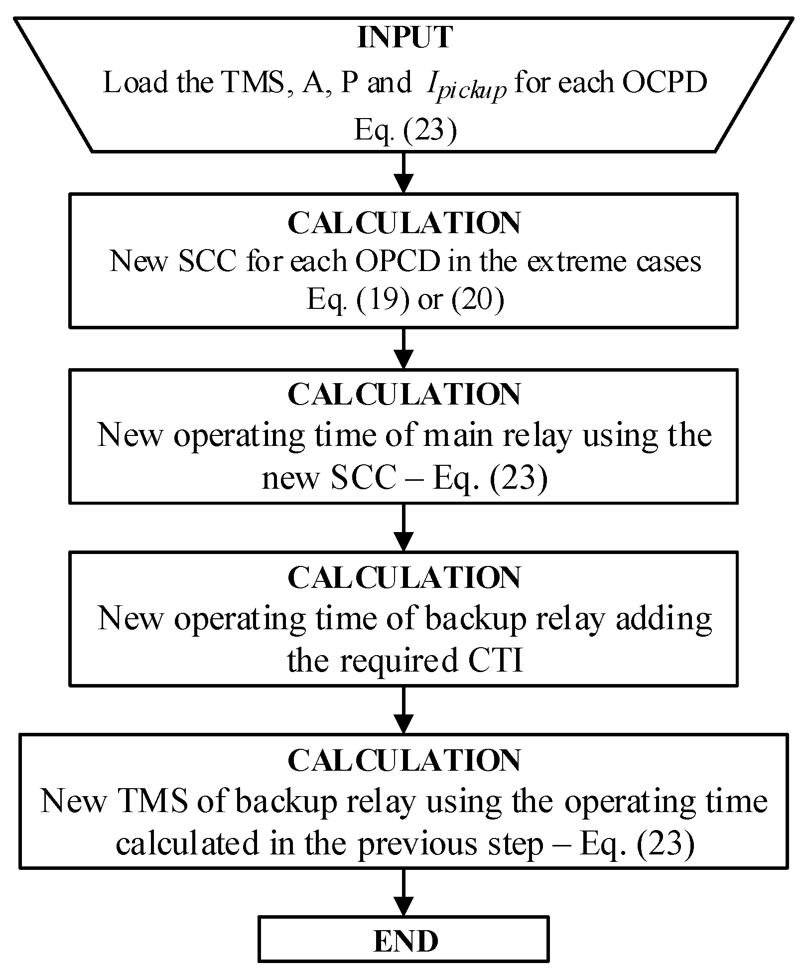
4.3. Adjustment of TMS

Another possible solution for the situation presented previously is to change the value of TMS. If the main and backup relays have the same inverse-time characteristic curve, the TMS of the backup relay can be increased to accommodate the minimum CTI between the devices for the new SCC level through them. The block diagram of this method is presented in Figure 8.
This method can also be applied to fuse–relay, relay–relay–relay, or fuse–relay–relay coordination, or in cases where it is possible to adjust the characteristic curve of the backup devices.

5. Case Study

To verify the proposed SCC estimation, the IEEE 34-Node Test Feeder was considered in this case study. This feeder was selected because it has similar characteristics to a real distribution feeder: unbalanced, extensive and single-phase laterals and connected distributed loads. Firstly, a classical overcurrent protection is proposed in this case study, including OCPD placement, relay and fuse settings, without considering the installation of IBRs. Subsequently, the contribution of SCC with IBRs is studied, and the results are compared with Simulink simulations. Additionally, the coordination of phase protection is evaluated, and a modification of the OCPD parameters is proposed.
The impacts on earth and fuse protection, reverse power flow and changes in the neutral current are beyond the scope of this work due to their complexity, and they may be addressed in future studies.

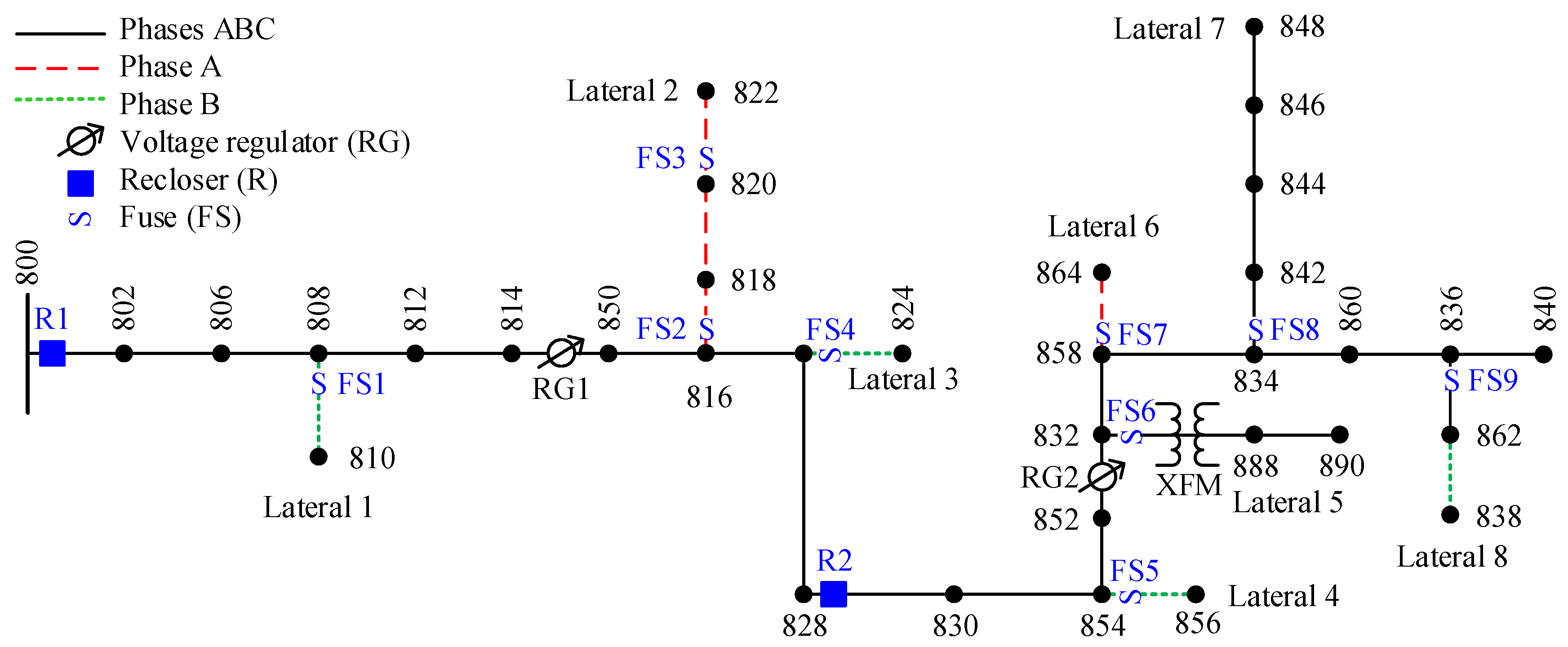
5.1. Overcurrent Protection for IEEE 34-Node Radial Test Feeder

5.1.1. Placing the OCPDs

Due to the characteristics of the feeder, two relays were utilized: R1, located near the substation (node 800), and R2 (node 828), situated 35.09 km from the substation. All the laterals were equipped with fuses (F#) at the beginning of the branch. The location of the OCPDs is shown in Figure 9. The OCPD parameters were determined using the data from the IEEE report, including the nominal and steady-state short-circuit currents. The conductors used were ACSR 1/0 bare conductors from node 800 to 814, and ACSR #2 6/1 bare conductors from node 814 to 840.

5.1.2. Fuse Settings

The fuses were determined using the following relations
i f u s e 1.5 I l o a d m a x
i f u s e 1 4 I p h m i n
where i f u s e represents the nominal fuse current, i l o a d m a x is the maximum load current that flows through the device on the installation site and I p h m i n represents the line-to-ground fault at the end of the protected lateral branch with a fault resistance of 20 Ω. Table 1 summarizes these values and presents the corresponding fuse links. Type K links were used for all lateral branches.

5.1.3. Relay Settings

Since both relays protect the fuses, they both have an extremely inverse (EI) curve characteristic, in accordance with IEC 60255 [40]. Table 2 summarizes the values of the maximum load current, maximum and minimum three-phase, double-phase and single-phase faults and neutral current flowing through R1 and R2.
The pickup currents for phase and earth faults ( I p u p h a s e and I p u e a r t h , respectively) can be given by
f g · I l o a d m a x < I p u p h a s e < I 2 p h m i n f s
I n < I p u e a r t h < I p h m i n
where f g is the growing demand factor (assumed to be 1.0), I 2 p h m i n is the minimum double line-to-line fault current, f s is the safety factor, which may vary from 1.5 up to 2.0 (assumed to be 2.0), I n is the neutral current and I p h m i n is the minimum phase-to-ground fault current. Therefore, the pickup currents for phase and earth protection must be between 51.56 A and 235.85 A, and 11.13 A and 135.3 A for relay R1; and 37.77 A and 108.15 A, and 4.55 A and 94.0 A for relay R2, respectively.
For phase protection, relay R2 must coordinate with the maximum fault current for the highest fuse downstream from it. The maximum fault current for fuse FS8-25K is 203.4 A, and its maximum clearing time is approximately 433.7 ms (according to S&C Electric Company’s “K” Speed Positrol Fuse Links Time-current Characteristics Curves). A CTI of 400 ms was chosen between the relay and fuse [41]. Therefore, for 203.4 A, R2 must operate at 833.7 ms. The appropriate pickup current for R2 must be at least three times the highest fuse downstream from it, which is 25 A. Therefore, the pickup current for R2 is equal to 75 A. For an EI curve, the TMS value is
0.8337 = T M S 80 203.4 75 2 1 T M S = 0.066
Then, the nearest available setting on the relay, TMS = 0.07, is used. Relay R1 needs to coordinate with R2 for a maximum current of 292.8 A through R2. R2 operates at 393.2 ms, so the pickup current of R1 should be equal to 90 A (120% of R2’s pickup) to ensure proper coordination between the relays. The appropriate CTI between R1 and R2 will be 300 ms [41]. Therefore, R1 must operate at 693.2 ms for 292.8 A. For an EI curve, the TMS value is
0.6932 = T M S 80 292.8 90 2 1 T M S = 0.083
Accordingly, TMS = 0.09 was considered. The coordination curves for phase protection are presented in Figure 10.
For earth fault protection, relay R2 must coordinate with the maximum fault current through fuse FS8, which is 158.3 A, and the maximum clearing time for this current is 722.8 ms. Thus, R2 must operate at 1122.8 ms, adding the appropriate CTI of 400 ms. For earth fault protection, the pickup current is typically set to 30–40% of the phase pickup. Therefore, the pickup current for R2 is 30 A. In this situation, for an EI curve, the TMS value would be
1.1228 = T M S 80 158.3 30 2 1 T M S = 0.376
TMS is then selected as 0.38. The relay R1 must coordinate with FS2-25 K for a fault current of 254.9 A, where the maximum clearing time for this current is 278.3 ms. Therefore, R1 must operate at 678.3 ms, considering the proper CTI of 400 ms. The pickup current for R1 is 40 A. In this scenario, for an EI curve, the TMS value is
0.6783 = T M S 80 254.9 40 2 1 T M S = 0.336
Considering the relay settings, TMS = 0.34 was selected. The coordination curves for earth fault protection are presented in Figure 11.
Table 3 provides a summary of the relay settings for the overcurrent protection of the IEEE 34-node test feeder, while Table 4 presents the coordination time intervals (CTIs) between relays and the highest fuses for both phase and earth protection. It is worth noting that the minimum CTIs of 300 ms between relays and 400 ms between relays and fuses have been observed.

5.2. Estimation of the Short-Circuit Current Contribution

Case studies were conducted on the IEEE 34-node test feeder to analyze a 3LG fault on the MFT and on lateral branches with integrated IBR. The results obtained from the proposed estimation method were compared with simulations in the MATLAB/Simulink environment using the IBR model suggested in previous studies [24,42,43,44]. The maximum SCC contribution of the IBR was set to 1.2 pu based on its base rating.

5.2.1. IBRs on the Main Fault Trunk

A 3LG fault was applied at node 840 of the IEEE 34-node test feeder (Figure 9), with Z f equal to 0 Ω and 20 Ω , and the currents were estimated and measured at R1 and R2 using the proposed estimation method and Simulink, respectively. This fault point was chosen to maintain the IBR connected during simulations because the adopted IBR model disconnects for points of common coupling (PCC) voltages under 0.1 pu of the nominal voltage.
According to IEEE data, the IEEE 34-node test feeder has a total power of 1769 kW of connected loads. Five situations of IBR penetration were evaluated: 0%, 25%, 50%, 75% and 100% of this total power, where 0% PL is used as a base for comparison. This total power was aggregated on a single three-phase IBR positioned at four different locations, including extremes, to evaluate the proposed estimation method.
  • IBR upstream R1 (right before)—Case 1;
  • IBR between R1 and R2 (righ after R1)—Case 2;
  • IBR between R1 and R2 (right before R2)—Case 3;
  • IBR downstream R2 (right after)—Case 4.
For each situation mentioned above, the currents on R1 and R2 were both estimated and measured for the two different values of Z f . The currents were then measured for the five different levels of IBR penetration. All the results are presented in Table 5.
For the base case (PL 0%), the average error between the Z f values was 1.5%, and this relative error decreased as the value of Z f increased. The errors were greater for R2 because the estimation method considers a pure fault circuit where the currents through R1 and R2 are equal, as presented in Section 2. On the other hand, the Simulink case considers the magnetic coupling, capacitance effect between the phases/neutral, the loads and capacitors connected, as well as the impact of single- and double-phase lateral branches. However, even under this scenario, the average error was within an acceptable range, according to the best knowledge of the authors.
For the cases with IBR penetration, on average, the error was 0.8%, and it was greater for Z f = 0 Ω (1.3%) and lower for Z f = 20 Ω (0.2%). The greatest errors between all the results were 3.2% (PL 100%, Case 4, R2, Z f = 0 Ω , Table 5) and −2.4% (PL 100%, Case 1, R1, Z f = 20 Ω , Table 5). The errors were within an acceptable range for protection studies, considering current transformer saturation.
Analyzing the current values, and comparing the cases with IBR penetration to the base, the greatest variations occurred for the 100% PL. For each PL analyzed, the highest and lowest currents for R1 occurred at Cases 1 and 2, respectively, and the highest and lowest for R2 occurred at Cases 3 and 4, respectively, as discussed in the sensitivity analysis in Section 3. These extreme values were also observed in Simulink simulations.
Even with a small SCC contribution (1.2 pu on the IBR’s base rating), the IBR can significantly change the current through the OCPDs. For example, for Z f = 0 Ω , Case 2, PL 100%, the current through R1 was −16.3% and −17.7% of the base for the estimation method and Simulink, respectively. For Case 3, under the same previous conditions, the current through R2 was 10.4% and 13.8% of the base for the estimation method and Simulink, respectively. Therefore, a high penetration of IBR caused a large current variation through the OCPDs, which may disrupt the protection of the feeder, depending on the settings, and should be investigated further.
For other scenarios, current variations greater than ±10% were also observed. Such variations outside of this range require attention in protection studies because they exceed the error range of devices, such as protection current transformers, and may impact the selectivity and coordination among the OCPDs. For instance, coordination may be lost due to a backup relay failing to trip (blind protection), tripping with a CTI lower than the minimum value (resulting in a higher SCC than without IBRs), or tripping faster than expected (disrupting a fuse-saving scheme and leading to a fuse-blow scheme).

5.2.2. IBRs on Lateral

In this case, the same 3LG fault was applied at node 840 of the IEEE 34-Node Test Feeder, with two different values of Z f , and for each case, five different levels of IBR penetration were considered: 0%, 25%, 50%, 75% and 100%. The 0% penetration level was used as the base case for comparison. Unlike the previous study, a single three-phase IBR was positioned at two different locations on Lateral 7 (refer to Figure 9):
  • IBR right after fuse FS8—Case Begin;
  • IBR at node 848—Case End.
With this, it is possible to evaluate whether the proposed equation for faults on the MFT for IBRs on laterals is suitable. Additionally, it can be seen whether the current value through FS8, in this case, is independent of the position of the IBR on the lateral branch and only dependent on the SCC value of the total amount of the IBRs downstream from it. Moreover, it is possible to evaluate whether the electrical distance of the lateral branch to the substation, according to the proposed estimation method, is sufficient to estimate the current through the OCPDs on the MFT (R1 and R2, in this case). All results are presented in Table 6, and all currents through FS8 flow reversely.
For the base case (PL 0%), the average error was 1.5%, and the difference between the current values of R1 and R2 is due to simulation characteristics, as explained previously. For the same reason, there is a difference between the estimation method and Simulink for currents through FS8: the method estimates a zero current through FS8 (because there is no IBR installed downstream of it), while Simulink returns a small value for all Z f values.
Considering only R1 and R2, for the cases with IBR penetration, there is a similar behavior when compared to the case only with an IBR on the MFT. The average error is greater for Z f = 0 Ω and decreases for Z f = 20 Ω , and as the PL increases, the average error decreases. For all these cases, the average error was 1.1%, showing good accuracy of the estimation method. The highest errors were 2.1% (PL 25%, Case Begin and End, R2, Z f = 0 Ω , Table 6) and −2.5% (PL 100%, Case Begin, R1, Z f = 20 Ω , Table 6). There was almost no difference in current values through R1 and R2 between the proposed estimation method and Simulink when the IBRs were installed at the beginning or end of the lateral branch, for all PLs and Z f . This supports the claim about the SCC contribution from IBRs on laterals while the fault is on the MFT.
Considering only FS8, for the cases with IBR penetration, the results were quite interesting. For all PLs with Z f = 0 Ω , the errors were extremely high because the IBR, in Simulink, was disconnected from the feeder due to the voltage sag at its PCC. For Z f = 20 Ω , the errors were high, but less than those for Z f = 0 Ω , and they decreased as the PL increased because the IBR remained connected during the fault with an SCC.
In this context, it should be noted that a reverse current through these devices in the case of a fault in the MFT may appear unexpectedly, and the estimation method can be a good alternative to estimate it—since, in the simulation, the IBR can be disconnected. Despite the high errors, the method estimates the worst current that can flow through an OCPD. If this current is higher than the current supported by the OCPD, changes may be made to ensure the coordination and reliability of the protection scheme.

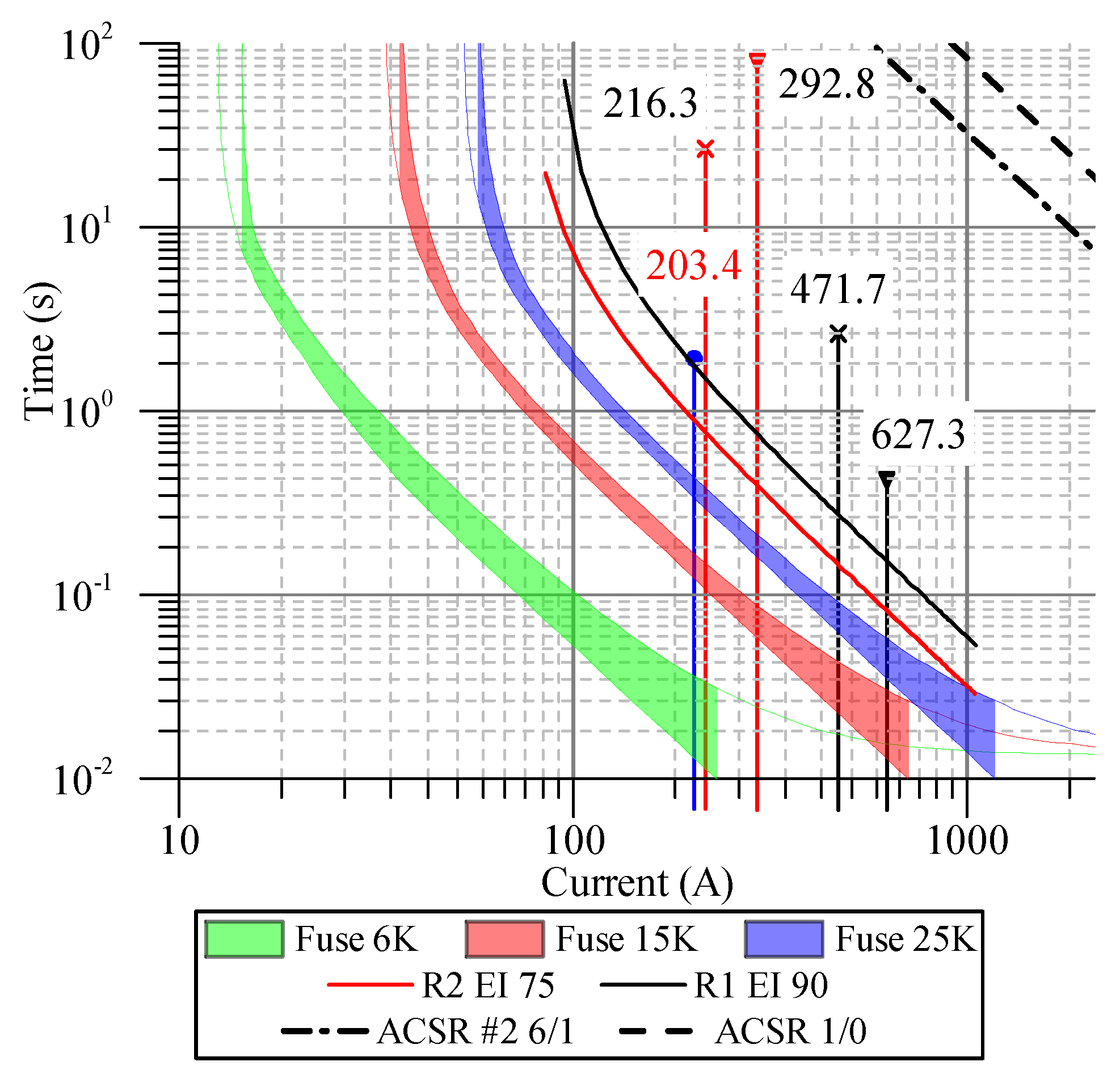
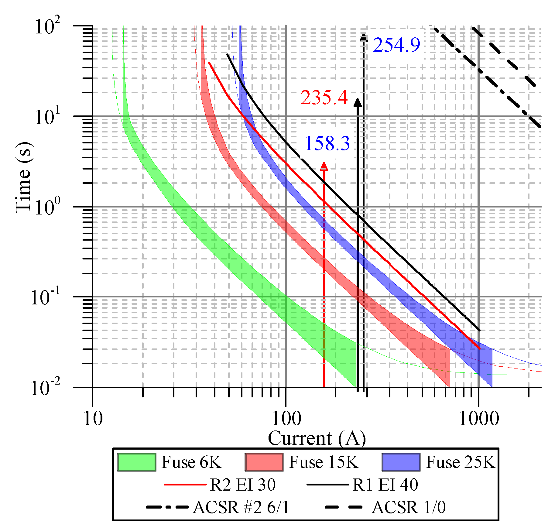
5.3. Impacts on the Actual Phase Protection Coordination Scheme

The impacts on the actual phase protection coordination scheme were analyzed for phase protection based on the CTI between devices for situations involving coordination between R1, R2 and FS8, considering a 100% PL of IBRs. Additionally, the impacts were evaluated considering that IBRs can inject an SCC of 1.2 pu and a maximum of 2.0 pu, given that some manufacturers are developing inverters with a higher magnitude and duration of the SCC contribution [9].
When the fault occurred at node 828, the CTI between R1 and R2 (Δt) without IBRs was equal to 329 ms, as presented in Table 7. For both values of the SCC contribution, the CTI between the devices decreased only for Case 1 due to the increase in SCC, but it remained above the minimum CTI of 300 ms. However, for an SCC of 2.0 pu, it was only 13 ms higher than the minimum CTI. This may impact the correct coordination between the devices on a real feeder. For Cases 2 and 3, with IBR between the devices, the CTIs were within an acceptable range, and the melting time of the conductors was not reached when the current was maximum for R2 and minimum for R1, as can be observed by comparing the values of the currents and the conductor curves in Figure 10.
When the fault occurred at node 834, the CTI between R2 and FS8 (the highest fuse downstream from R2) without IBRs was equal to 472 ms, as presented in Table 8. Case 5 represents the scenario when the IBR is located right before FS8, and Case 6 when the IBR is located right after FS8. Cases 1 to 4 are the same as before. The coordination was lost between R2 and FS8 for Case 3 for both SCC contributions. For 1.2 pu, the CTI reached 365 ms, and for 2.0 pu, it was 309 ms, below the minimum CTI of 400 ms. For the other cases, the CTI between R2 and FS8 was within an acceptable range, not disrupting the melting time of the conductor.
Since coordination was lost, an adjustment to the actual coordination scheme must be made for phase protection, starting with the coordination of R2 and FS8 for a fault at node 834 and then for R1 and R2 for a fault at node 828.

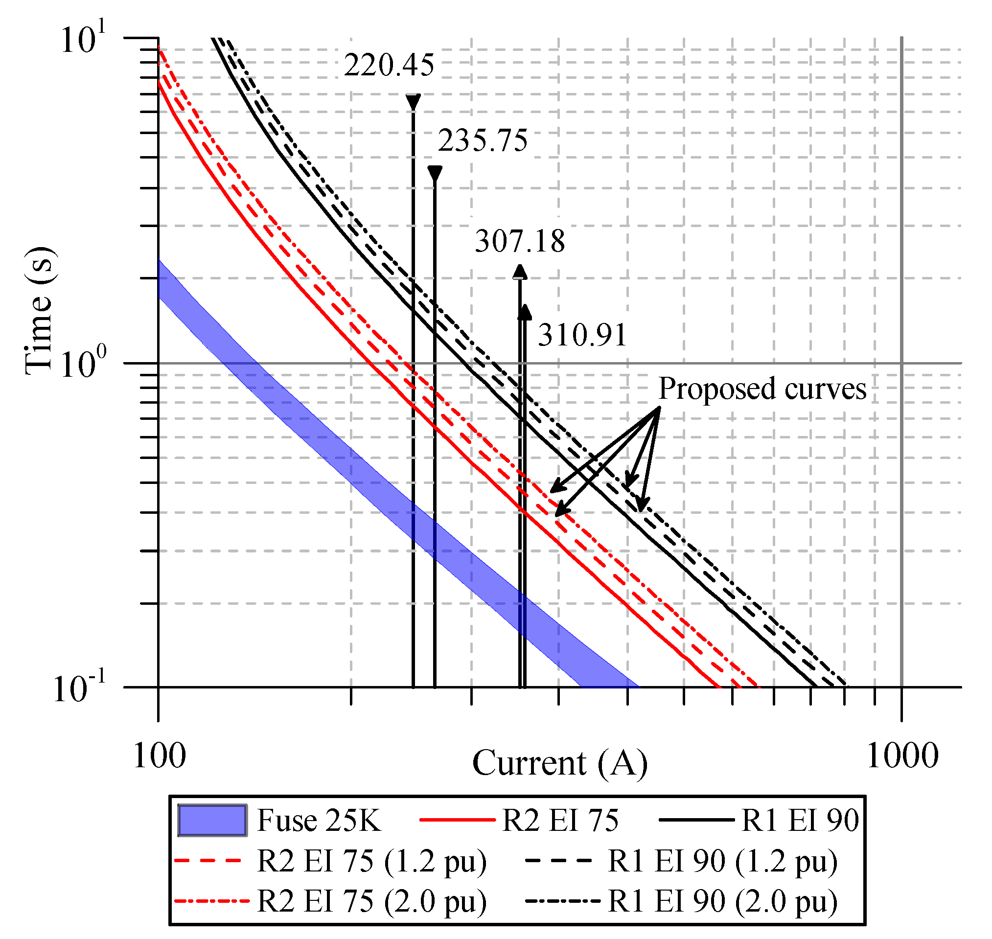
5.4. Changing the Actual Phase Protection Scheme

For this adjustment, the slope of the R1 and R2 curves was maintained. The change will be made to the TMS setting according to the block-diagram presented in Figure 8 since the conductor’s melting time was not reached for any cases with IBRs between the OCPDs. The new settings are presented in Table 9.
For an SCC contribution of 1.2 pu, the maximum current through R2 and FS8 was 220.45 A. For this current, FS8 operates at 365 ms, and to ensure a minimum 400 ms CTI, R2 must operate at 770 ms, considering the same previous EI characteristic curve and pickup current. Then, the new TMS was equal to 0.08. Between R1 and R2, the maximum current was 307.18 A. For this current, R2 operates at 406 ms, and to ensure the minimum 300 ms CTI, R1 must operate at 706 ms, considering the same previous EI characteristic curve and pickup current. Then, the new TMS was equal to 0.1. Note that both TMS values were higher than before, causing the curves to move upward graphically, delaying their operation for the previous maximum fault currents.
For 2.0 pu, the new TMS was 0.09 for R2 and 0.11 for R1, higher than for 1.2 pu SCC contribution. The proposed curves are presented in Figure 12.

5.5. Assertiveness of the New Phase Protection Scheme

The results for the new protection scheme at coordination currents are presented in Table 10. As can be seen, the CTI between R2 and FS8 increased from 365 ms (Table 8—Case 3) to 470 ms for 1.2 pu of SCC contribution, and from 309 ms (Table 8—Case 3) to 489 ms for 2.0 pu of the SCC contribution. Additionally, between R1 and R2, the CTI increased from 321 ms (Table 7—Case 1) to 346 ms, and from 313 ms (Table 7—Case 1) to 360 ms for 1.2 pu and 2.0 pu of SCC contribution, respectively, thereby ensuring a good operation margin between the devices than before.
The proposed changes have increased the reliability of the phase protection of the feeder, ensuring its protection up to 100% of PL from IBRs. Furthermore, choosing values for the 2.0 pu of the SCC contribution may offer a good operation margin for the OCPDs, considering that there are SCC contributions from loads and capacitor banks, which are outside the scope of this method.
The impacts on the OCPDs installed on the MFT and those installed on laterals, with the presence of IBRs, were analyzed, and the accuracy of the method was within an acceptable range for the current error. Moreover, the method aims to estimate the worst SCC contribution to perform a protection coordination between adjacent devices. For SCC contributions below the worst estimated contribution, the OCPDs will be coordinated.
Additionally, the proposed methodologies can be extended to other feeders and serve as an evaluation tool for DNOs to plan the grid operation in the design phase. They can also be used by teachers and in protection courses to illustrate the impacts on the SCC of a feeder in a more simplified and didactic way. The present study contributes to the enhancement of protection coordination in distribution networks with high penetration levels of IBRs. The practical implications and findings of this research hold significant relevance for distribution system operators and planners who are committed to ensuring the safety and reliability of distribution feeders.

6. Conclusions

This paper proposes a practical methodology to estimate the contribution of SCC on distribution feeders with IBRs. The results show an average error of 1.5% in estimating SCCs through OCPDs installed on the MFT and on lateral branches, considering the IBRs installation location and a penetration level up to 100%. The maximum error of the method was 3.0% for OCPDs installed on the MFT when the IBRs are installed on the MFT or lateral branches. For OCPDs installed on lateral branches, a reverse SCC was observed, resulting in larger errors. However, the values were still within an acceptable range for the phase coordination objective. Additionally, for a high PL, the small SCC contribution of IBRs disrupted the phase protection coordination of the feeder. A methodology to restore the lost phase protection coordination was proposed by using the estimated SCC values to adjust the TMS of the OCPDs. A proposal was made to restore the phase protection for an SCC of 1.2 pu and 2.0 pu from IBRs. These methodologies can be used by Distribution Network Operators (DNOs) to estimate the critical SCC values of a feeder and adjust the phase protection coordination to avoid a miscoordination or malfunction of the system protection. This research contributes to enhancing the protection coordination of distribution networks with high penetration levels of IBRs. The practical implications and findings of this study are relevant to distribution system operators and planners who aim to ensure the safety and reliability of distribution feeders.

Author Contributions

Conceptualization, M.C.V.; methodology, M.C.V.; software, M.C.V.; validation, M.C.V.; formal analysis, M.C.V.; investigation, M.C.V.; data curation, M.C.V.; writing—original draft preparation, M.C.V.; writing—review and editing, M.C.V., O.E.B. and Y.Y.; supervision, O.E.B. and Y.Y.; project administration, M.C.V. All authors have read and agreed to the published version of the manuscript.

Funding

This study was supported in part by the Coordenação de Aperfeiçoamento de Pessoal de Nível Superior-Brazil (CAPES)-Finance Code 001. This work was carried out with the support of the Espírito Santo Research and Innovation Support Foundation (Fapes).

Data Availability Statement

The data presented in this study are available on request from the corresponding author.

Acknowledgments

M.C. Vargas thanks Federal Institute of Espirito Santo (IFES) for the financial and institutional support during the completion of the doctorate course in electrical engineering.

Conflicts of Interest

The authors declare no conflict of interest.

Abbreviations

The following abbreviations are used in this manuscript:
3LGThree-phase line-to-ground
ACSRAluminium-conductor steel-reinforced
CTICoordination time interval
CSICurrent source inverter
DERsDistributed energy resources
DNDistribution network
DNODistribution network operator
EIExtreme inverse
FSFuse
IBRsInverter-based resources
MFTMain fault trunk
OCPDsOvercurrent protection devices
PCCPoint of common coupling
PLPenetration level
PVPhotovoltaic
SCCShort-circuit current
TMSTime multiplies settings

References

  1. Lew, D.; Asano, M.; Boemer, J.; Ching, C.; Focken, U.; Hydzik, R.; Lange, M.; Motley, A. The Power of Small: The Effects of Distributed Energy Resources on System Reliability. IEEE Power Energy Mag. 2017, 15, 50–60. [Google Scholar] [CrossRef]
  2. Vargas, M.C.; Mendes, M.A.; Batista, O.E. Fault Current Analysis on Distribution Feeders with High Integration of Small Scale PV Generation. In Proceedings of the 2019 IEEE Power & Energy Society General Meeting (PESGM), Atlanta, GA, USA, 4–8 August 2019; pp. 1–5. [Google Scholar] [CrossRef]
  3. Meskin, M.; Domijan, A.; Grinberg, I. Impact of distributed generation on the protection systems of distribution networks: Analysis and remedies-review paper. IET Gener. Transm. Distrib. 2020, 14, 5944–5960. [Google Scholar] [CrossRef]
  4. Kou, G.; Chen, L.; Vansant, P.; Velez-Cedeno, F.; Liu, Y. Fault Characteristics of Distributed Solar Generation. IEEE Trans. Power Deliv. 2020, 35, 1062–1064. [Google Scholar] [CrossRef]
  5. Barker, P.P.; De Mello, R.W. Determining the impact of distributed generation on power systems. I. Radial distribution systems. In Proceedings of the 2000 Power Engineering Society Summer Meeting, Seattle, DC, USA, 16–20 July 2000; Volume 3, pp. 1645–1656. [Google Scholar] [CrossRef]
  6. Baran, M.E.; El-Markaby, I. Fault Analysis on Distribution Feeders with Distributed Generators. IEEE Trans. Power Syst. 2005, 20, 1757–1764. [Google Scholar] [CrossRef]
  7. Keller, J.; Kroposki, B. Understanding Fault Characteristics of Inverter-Based Distributed Energy Resources; Technical Report; National Renewable Energy Laboratory (NREL): Golden, CO, USA, 2010. [Google Scholar] [CrossRef] [Green Version]
  8. Dugan, R.C.; McDermott, T.E. Distributed generation. IEEE Ind. Appl. Mag. 2002, 8, 19–25. [Google Scholar] [CrossRef]
  9. Reno, M.J.; Brahma, S.; Bidram, A.; Ropp, M.E. Influence of Inverter-Based Resources on Microgrid Protection: Part 1: Microgrids in Radial Distribution Systems. IEEE Power Energy Mag. 2021, 19, 36–46. [Google Scholar] [CrossRef]
  10. Manson, S.; McCullough, E. Practical Microgrid Protection Solutions: Promises and Challenges. IEEE Power Energy Mag. 2021, 19, 58–69. [Google Scholar] [CrossRef]
  11. IEEE Power & Energy Society. PES-TR67.r1—Impact of IEEE 1547 Standard on Smart Inverters and the Applications in Power Systems; Technical Report August; IEEE PES: Piscataway, NJ, USA, 2020. [Google Scholar]
  12. Bhagavathy, S.; Pearsall, N.; Putrus, G.; Walker, S. Performance of UK Distribution Networks with single-phase PV systems under fault. Int. J. Electr. Power Energy Syst. 2019, 113, 713–725. [Google Scholar] [CrossRef]
  13. IEEE Std 1547–2018; IEEE Standard for Interconnection and Interoperability of Distributed Energy Resources with Associated Electric Power Systems Interfaces. IEEE: Piscataway, NJ, USA, 2018; pp. 1547–2018. [CrossRef]
  14. Key, T.; Kou, G.; Jensen, M. On Good Behavior: Inverter-Grid Protections for Integrating Distributed Photovoltaics. IEEE Power Energy Mag. 2020, 18, 75–85. [Google Scholar] [CrossRef]
  15. Blaabjerg, F.; Yang, Y.; Yang, D.; Wang, X. Distributed Power-Generation Systems and Protection. Proc. IEEE 2017, 105, 1311–1331. [Google Scholar] [CrossRef] [Green Version]
  16. Mendes, M.A.; Vargas, M.C.; Simonetti, D.S.L.; Batista, O.E. Load Currents Behavior in Distribution Feeders Dominated by Photovoltaic Distributed Generation. Electr. Power Syst. Res. 2021, 201, 107532. [Google Scholar] [CrossRef]
  17. Nassif, A.B. An Analytical Assessment of Feeder Overcurrent Protection with Large Penetration of Distributed Energy Resources. IEEE Trans. Ind. Appl. 2018, 54, 5400–5407. [Google Scholar] [CrossRef]
  18. Razavi, S.; Rahimi, E.; Javadi, M.S.; Nezhad, A.E.; Lotfi, M.; Shafie-khah, M.; Catalão, J.P.S. Impact of distributed generation on protection and voltage regulation of distribution systems: A review. Renew. Sustain. Energy Rev. 2019, 105, 157–167. [Google Scholar] [CrossRef]
  19. Haddadi, A.; Farantatos, E.; Kocar, I.; Karaagac, U. Impact of Inverter Based Resources on System Protection. Energies 2021, 14, 1050. [Google Scholar] [CrossRef]
  20. Chae, W.; Lee, J.H.; Kim, W.H.; Hwang, S.; Kim, J.O.; Kim, J.E. Adaptive Protection Coordination Method Design of Remote Microgrid for Three-Phase Short Circuit Fault. Energies 2021, 14, 7754. [Google Scholar] [CrossRef]
  21. Simic, N.; Strezoski, L.; Dumnic, B. Short-Circuit Analysis of DER-Based Microgrids in Connected and Islanded Modes of Operation. Energies 2021, 14, 6372. [Google Scholar] [CrossRef]
  22. Kim, I. Steady-state short-circuit current calculation for internally limited inverter-based distributed generation sources connected as current sources using the sequence method. Int. Trans. Electr. Energy Syst. 2019, 29, e12125. [Google Scholar] [CrossRef]
  23. Plet, C.A.; Green, T.C. Fault response of inverter interfaced distributed generators in grid-connected applications. Electr. Power Syst. Res. 2014, 106, 21–28. [Google Scholar] [CrossRef]
  24. Mendes, M.A.; Vargas, M.C.; Batista, O.E.; Yang, Y.; Blaabjerg, F. Simplified Single-phase PV Generator Model for Distribution Feeders with High Penetration of Power Electronics-based Systems. In Proceedings of the 2019 IEEE 15th Brazilian Power Electronics Conference and 5th IEEE Southern Power Electronics Conference, COBEP/SPEC, Santos, Brazil, 1–4 December 2019; pp. 1–7. [Google Scholar] [CrossRef]
  25. Dash, P.P.; Kazerani, M. Dynamic modeling and performance analysis of a grid-connected current-source inverter-based photovoltaic system. IEEE Trans. Sustain. Energy 2011, 2, 443–450. [Google Scholar] [CrossRef]
  26. Seuss, J.; Reno, M.J.; Broderick, R.J.; Grijalva, S. Determining the Impact of Steady-State PV Fault Current Injections on Distribution Protection; Technical Report; Sandia National Laboratories (SNL): Golden, CO, USA, 2017. [Google Scholar] [CrossRef]
  27. Cho, N.; Yun, S.; Jung, J. Shunt fault analysis methodology for power distribution networks with inverter-based distributed energy resources of the Korea Electric Power Corporation. Renew. Sustain. Energy Rev. 2020, 133, 110140. [Google Scholar] [CrossRef]
  28. Kim, I. Short-Circuit Analysis Models for Unbalanced Inverter-Based Distributed Generation Sources and Loads. IEEE Trans. Power Syst. 2019, 34, 3515–3526. [Google Scholar] [CrossRef]
  29. Kim, I. A calculation method for the short-circuit current contribution of current-control inverter-based distributed generation sources at balanced conditions. Electr. Power Syst. Res. 2021, 190, 106839. [Google Scholar] [CrossRef]
  30. Strezoski, L.; Prica, M.; Loparo, K.A. Generalized δ-Circuit Concept for Integration of Distributed Generators in Online Short-Circuit Calculations. IEEE Trans. Power Syst. 2017, 32, 3237–3245. [Google Scholar] [CrossRef]
  31. Strezoski, L.; Prica, M.; Loparo, K.A. Sequence Domain Calculation of Active Unbalanced Distribution Systems Affected by Complex Short Circuits. IEEE Trans. Power Syst. 2018, 33, 1891–1902. [Google Scholar] [CrossRef]
  32. Strezoski, L.; Stefani, I.; Bekut, D. Novel method for adaptive relay protection in distribution systems with electronically-coupled DERs. Int. J. Electr. Power Energy Syst. 2020, 116, 105551. [Google Scholar] [CrossRef]
  33. Tonini, L.G.R.; Freire, R.S.F.; Batista, O.E. Load Flow and Short-Circuit Methods for Grids Dominated by Inverter-Based Distributed Generation. Energies 2022, 15, 4723. [Google Scholar] [CrossRef]
  34. IEC 60909-0:2016; Short-Circuit Currents in Three-Phase a.c. Systems—Part 0: Calculation of Currents. 2016. Available online: https://webstore.iec.ch/publication/24100#:~:text=IEC%2060909%2D0%3A2016%20is,50%20Hz%20or%2060%20Hz (accessed on 18 February 2023).
  35. IEEE Std 242-2001; IEEE Recommended Practice for Protection and Coordination of Industrial and Commercial Power Systems. IEEE: Piscataway, NJ, USA, 2001.
  36. Anderson, P.M. Power System Protection; McGraw-Hill: New York, NY, USA, 1999; p. 1307. [Google Scholar]
  37. Horowitz, S.; Phadke, A.; Henville, C. Power System Relaying; Wiley: Hoboken, NJ, USA, 2022. [Google Scholar]
  38. Gers, J.; Holmes, E. Protection of Electricity Distribution Networks, 2nd ed.; IET: London, UK, 2004. [Google Scholar]
  39. Fani, B.; Bisheh, H.; Sadeghkhani, I. Protection coordination scheme for distribution networks with high penetration of photovoltaic generators. IET Gener. Transm. Distrib. 2018, 12, 1802–1814. [Google Scholar] [CrossRef]
  40. IEC 60255-151:2009; Measuring Relays and Protection Equipment—Part 151: Functional Requirements for over/under Current Protection. IEEE: Piscataway, NJ, USA, 2009.
  41. Systems, C.P. Electrical Distribution-System Protection: A Textbook and Practical Reference on Overcurrent and Overvoltage Fundamentals, Protective Equipment and Applications; Cooper Power Systems: Pewaukee, WI, USA, 2005. [Google Scholar]
  42. Vargas, M.C.; Mendes, M.A.; Tonini, L.G.R.; Batista, O.E. Grid Support of Small-scale PV Generators with Reactive Power Injection in Distribution Systems. In Proceedings of the 2019 IEEE PES Innovative Smart Grid Technologies Conference—Latin America (ISGT Latin America), Washington, DC, USA, 15–18 September 2019; IEEE: Gramado, Brazil, 2019; pp. 1–6. [Google Scholar] [CrossRef]
  43. Ferraz, R.S.F.; Ferraz, R.S.F.; Rueda-Medina, A.C.; Batista, O.E. Genetic optimisation-based distributed energy resource allocation and recloser-fuse coordination. IET Gener. Transm. Distrib. 2020, 14, 4501–4508. [Google Scholar] [CrossRef]
  44. Matos, S.P.S.; Vargas, M.C.; Fracalossi, L.G.V.; Encarnação, L.F.; Batista, O.E. Protection philosophy for distribution grids with high penetration of distributed generation. Electr. Power Syst. Res. 2021, 196, 107203. [Google Scholar] [CrossRef]
Figure 1. Single-line diagram of a radial distribution feeder, with two OCPDs, dominated by IBRs, and a three-phase line-to-ground fault at point F.
Energies 16 03130 g001
Figure 2. Radial distribution feeder with the integration of IBRs and a 3LG fault (F1) at bus 3.
Energies 16 03130 g002
Figure 3. Radial distribution feeder with the integration of IBRs and a 3LG fault (F2) at bus 4.
Energies 16 03130 g003
Figure 4. Block-diagram of the proposed SCC calculation method.
Energies 16 03130 g004
Figure 5. Hypothetical extreme situations for fault currents through OCPDs in a high penetration scenario of IBRs.
Energies 16 03130 g005
Figure 6. Overcurrent protection coordination between OCPD1 and OCPD2 with only IBRs between.
Energies 16 03130 g006
Figure 7. Strategy to restore the protection coordination between two OCPDs in a distribution feeder dominated by IBRs.
Energies 16 03130 g007
Figure 8. Block-diagram of the proposed TMS adjustment.
Energies 16 03130 g008
Figure 9. Single-line diagram of the IEEE 34-node test feeder with OCPDs.
Energies 16 03130 g009
Figure 10. Phase fault protection coordination for R1 (in black), R2 (in red) and fuses 6 K, 15 K and 25 K. The vertical lines represent fault currents: downwards triangle is a 3LG fault, X is a phase-to-phase fault and circle is the maximum fault through the highest fuse for R2. The SCC damage curves for ACSR 1/0 and #2 6/1 bare conductors are also represented.
Energies 16 03130 g010
Figure 11. Earth fault protection coordination for R1 (in black), R2 (in red) and fuses 6 K, 15 K and 25 K. The vertical lines represent fault currents: upwards triangle is a line-to-earth fault. The SCC damage curves for ACSR 1/0 and #2 6/1 bare conductors are also represented.
Energies 16 03130 g011
Figure 12. Modified phase fault protection coordination for R1 (in black), R2 (in red) and fuse 25 K, considering a 100% PL of IBRs and different SCC contribution capacities on IBR’s base rating. The continuous curves represent the protection coordination without IBRs.
Energies 16 03130 g012
Table 1. Maximum load currents, minimum line-to-ground faults and fuse link to protect laterals on the IEEE 34-node test feeder.
Max. Load
Current (A)
Min. Line-to-Ground
Fault (A)
Fuse Link
FS11.22298.006 K
FS213.02135.3025 K
FS310.62135.3015 K
FS43.10190.406 K
FS50.31148.006 K
FS611.7094.0020 K
FS70.14139.406 K
FS816.30133.6025 K
FS92.09131.406 K
Table 2. Load and fault currents through R1 and R2 on the IEEE 34-node test feeder.
Max. Load
Current
(A)
Max. Three
Phase Fault
(A)
Max. Double
Phase Fault
(A)
Max. Single
Phase Fault
(A)
Min. Three
Phase Fault
(A)
Min. Double
Phase Fault
(A)
Min. Single
Phase Fault
(A)
Neutral
Current
(A)
R151.56627.3543.3655.2439.9471.7135.311.13
R237.77292.8253.8235.4221.0216.3131.44.55
Table 3. Relays settings.
Phase
Protection
Earth
Protection
R1Pickup (A)9040
Curve – IEC 60255EIEI
TMS0.090.34
R2Pickup (A)7530
Curve – IEC 60255EIEI
TMS0.070.38
Table 4. CTI between relays and fuses FS2 and FS8 for maximum and minimum fault types on the IEEE 34-node test feeder.
ABFault (A)
3LG
A Tripping
Time (ms)
B Tripping
Time (ms)
CTI (ms)
(A–B)
Fault (A)
2L
A Tripping
Time (ms)
B Tripping
Time (ms)
CTI (ms)
(A–B)
R1R2Max.292.8751.2393.2358.0Max.253.81035.6535.8499.8
Min.221.01431.5728.9702.6Min.216.31507.5765.3742.2
R2FS8Max.203.4881.2433.7447.5Max.175.01260.0588.1671.9
Min.159.31594.8714.0880.8Min.152.81777.4779.7997.6
ABFault (A)
LG (start)
A Tripping
Time (ms)
B Tripping
Time (ms)
CTI (ms)
(A–B)
Fault (A)
LG (end)
A Tripping
Time (ms)
B Tripping
Time (ms)
CTI (ms)
(A–B)
R1R2Max.235.4808.7501.9306.8Max.150.72061.51254.4807.1
Min.194.01207.7744.8462.9Min.131.42778.01671.81106.2
FS2Max.254.9686.7278.3408.4Max.157.31880.5731.61148.8
Min.207.91045.6416.3629.3Min.135.32605.01020.11584.9
R2FS8Max.158.31132.5722.8409.7Max.154.01199.2765.7433.4
Min.137.01531.1992.0539.1Min.133.61614.31048.1566.1
Table 5. Currents Through R1 and R2 for a 3LG Fault at Node 840 on the IEEE 34-Node Test Feeder and IBR Located on the MFT for Different Penetration Levels (PL) and Fault Resistances ( Z f ).
Z f = 0 Ω Z f = 20 Ω Error (%)
PLCase Method Simulink Method Simulink Method/
Current Current Current Current Simulink
(A)%(A)%(A)%(A)% 0 Ω 20 Ω
0%R1199.91-197.66-164.41-164.42-1.1%0.0%
R2199.91-195.20-164.41-161.08-2.4%2.1%
25%1R1200.360.2%199.671.0%164.790.2%166.381.2%0.3%−1.0%
R2200.360.2%196.640.7%164.790.2%162.460.9%1.9%1.4%
2R1191.53−4.2%189.23−4.3%154.71−5.9%155.38−5.5%1.2%−0.4%
R2200.360.2%196.640.7%164.790.2%162.460.9%1.9%1.4%
3R1195.86−2.0%194.16−1.8%158.27−3.7%159.23−3.2%0.9%−0.6%
R2204.832.5%202.373.7%168.462.5%167.103.7%1.2%0.8%
4R1195.86−2.0%194.16−1.8%158.27−3.7%159.23−3.2%0.9%−0.6%
R2195.86−2.0%191.09−2.1%158.27−3.7%155.25−3.6%2.5%1.9%
50%1R1200.870.5%200.771.6%165.210.5%167.221.7%0.0%−1.2%
R2200.870.5%197.731.3%165.210.5%163.281.4%1.6%1.2%
2R1183.30−8.3%180.13−8.9%145.14−11.7%145.51−11.5%1.8%−0.3%
R2200.870.5%197.731.3%165.210.5%163.281.4%1.6%1.2%
3R1191.84−4.0%189.85−4.0%152.15−7.5%152.97−7.0%1.0%−0.5%
R2209.945.0%209.117.1%172.665.0%172.537.1%0.4%0.1%
4R1191.84−4.0%189.85−4.0%152.15−7.5%152.97−7.0%1.0%−0.5%
R2191.84−4.0%186.71−4.3%152.15−7.5%148.90−7.6%2.7%2.2%
75%1R1201.440.8%201.822.1%165.670.8%168.022.2%−0.2%−1.4%
R2201.440.8%198.761.8%165.670.8%164.061.9%1.3%1.0%
2R1175.24−12.3%171.24−13.4%135.72−17.5%135.88−17.4%2.3%−0.1%
R2201.440.8%198.761.8%165.670.8%164.061.9%1.3%1.0%
3R1187.83−6.0%185.59−6.1%146.04−11.2%146.70−10.8%1.2%−0.4%
R2215.247.7%215.7010.5%177.027.7%177.8810.4%−0.2%−0.5%
4R1187.83−6.0%185.59−6.1%146.04−11.2%146.70−10.8%1.2%−0.4%
R2187.83−6.0%182.40−6.6%146.04−11.2%142.56−11.5%3.0%2.4%
100%1R1202.061.1%202.822.6%166.191.1%168.772.6%−0.4%−1.5%
R2202.061.1%199.752.3%166.191.1%164.792.3%1.2%0.8%
2R1167.38−16.3%162.62−17.7%126.50−23.1%126.52−23.0%2.9%0.0%
R2202.061.1%199.752.3%166.191.1%164.792.3%1.2%0.8%
3R1183.85−8.0%181.40−8.2%139.96−14.9%140.43−14.6%1.4%−0.3%
R2220.7010.4%222.1513.8%181.5210.4%183.1413.7%−0.7%−0.9%
4R1183.85−8.0%181.40−8.2%139.96−14.9%140.43−14.6%1.4%−0.3%
R2183.85−8.0%178.15−8.7%139.96−14.9%136.22−15.4%3.2%2.7%
The % on each Z f refers to each base case (0%). The % of relative errors on error columns are given comparing the respective values of the estimation method with Simulink simulation at each Z f : Case 1—IBR upstream R1 (right before); Case 2—IBR between R1 and R2 (righ after R1); Case 3—IBR between R1 and R2 (right before R2); Case 4—IBR downstream R2 (right after).
Table 6. Currents Through R1 and R2 for a 3LG Fault at Node 840 on IEEE 34-Node Test Feeder and IBR Located on the Lateral 7 for Different Penetration Levels (PL) and Fault Resistances ( Z f ).
Z f = 0 Ω Z f = 20 Ω Error (%)
PLCase Method Simulink Method Simulink Method/
Current Current Current Current Simulink
(A)%(A)%(A)%(A)% 0 Ω 20 Ω
0%R1199.91-198.51-164.41-165.49-0.7%−0.6%
R2199.91-195.50-164.41-161.59-2.3%1.7%
FS80.00-0.41-0.00-3.55-−100.0%−100.0%
25%BeginR1199.60−0.2%198.510.0%161.35−1.9%163.22−1.4%0.5%−1.1%
R2199.60−0.2%195.500.0%161.35−1.9%159.27−1.4%2.1%1.3%
FS812.31-0.410.0%12.31-9.78175.2%2938.0%25.9%
EndR1199.60−0.2%198.510.0%161.35−1.9%163.22−1.4%0.5%−1.1%
R2199.60−0.2%195.500.0%161.35−1.9%159.27−1.4%2.1%1.3%
FS812.31-0.410.0%12.31-9.77175.0%2938.0%25.9%
50%BeginR1199.30−0.3%198.510.0%158.28−3.7%160.88−2.8%0.4%−1.6%
R2199.30−0.3%195.500.0%158.28−3.7%156.87−2.9%1.9%0.9%
FS824.61-0.410.0%24.61-21.72511.3%5975.9%13.3%
EndR1199.30−0.3%198.510.0%158.28−3.7%160.86−2.8%0.4%−1.6%
R2199.30−0.3%195.500.0%158.28−3.7%156.86−2.9%1.9%0.9%
FS824.61-0.410.0%24.61-21.71510.9%5975.9%13.4%
75%BeginR1199.00−0.5%198.510.0%155.22−5.6%158.46−4.2%0.2%−2.0%
R2199.00−0.5%195.500.0%155.22−5.6%154.41−4.4%1.8%0.5%
FS836.92-0.410.0%36.92-33.77850.5%9013.9%9.3%
EndR1199.00−0.5%198.510.0%155.22−5.6%158.42−4.3%0.2%−2.0%
R2199.00−0.5%195.500.0%155.22−5.6%154.36−4.5%1.8%0.6%
FS836.92-0.410.0%36.92-33.75849.9%9013.9%9.4%
100%BeginR1198.69−0.6%198.510.0%152.15−7.5%155.98−5.7%0.1%-2.5%
R2198.69−0.6%195.500.0%152.15−7.5%151.87−6.0%1.6%0.2%
FS849.22-0.410.0%49.22-45.851190.4%12,051.8%7.4%
EndR1198.69−0.6%198.510.0%152.15−7.5%155.90−5.8%0.1%−2.4%
R2198.69−0.6%195.500.0%152.15−7.5%151.79−6.1%1.6%0.2%
FS849.22-0.410.0%49.22-45.821189.6%12,051.8%7.4%
The % on each Z f are refereed to each base case (0%). The % on relative errors on error columns are given comparing the respective values of estimation method with Simulink simulation at each Z f .
Table 7. Tripping Times for R1 and R2 for a Fault at Node 828 of the IEEE 34-Node Test Feeder with 100% of Penetration Level of IBRs.
IBR
SCC
CaseR1
(A)
R2
(A)
R1
(ms)
R2
(ms)
Δt
(ms)
0 pu-303.91303.91692363329
1.2 pu1307.18307.18676355321
2277.86307.18844355489
3300.63332.07709301408
4300.63300.63709372337
2.0 pu1310.91310.91659346313
2261.33310.91969346623
3298.45352.93720265455
4298.45298.45720377343
Case 1—IBR upstream R1 (right before); Case 2—IBR between R1 and R2 (righ after R1); Case 3—IBR between R1 and R2 (right before R2); Case 4—IBR downstream R2 (right after).
Table 8. Tripping Times for R1, R2 and FS8 for a Fault at Node 834 of the IEEE 34-Node Test Feeder with 100% Penetration Level of IBRs.
IBR
SCC
CaseR1
(A)
R2
(A)
FS8
(A)
R1 Trip
(ms)
R2 Trip
(ms)
FS8 Trip
(ms)
Δt (R1-R2)
(ms)
Δt (R2-FS8)
(ms)
0 pu-199.68199.68199.681836920448916472
1.2 pu1201.83201.83201.831787897439890458
2167.14201.83201.8329408974392043458
3183.59220.45220.4522787333681545365
4183.59183.59220.45227811223681156754
5198.41198.41236.291865934321932613
6198.41198.41198.411865934455932479
2.0 pu1203.77203.77203.771745878432867446
2147.37203.77203.7742838784323405446
3173.10235.75235.7526676313222037309
4173.10173.10235.75266712943221373972
5197.56197.56262.711885943263942680
6197.57197.57197.571885943459942484
Table 9. Relay Settings for Phase Protection of the IEEE 34-Node Test Feeder with 100% PL of IBRs.
IBR with SCC
of 1.2 pu
IBR with SCC
of 2.0 pu
R1Pickup (A)9090
Curve-IEC 60255EIEI
TMS0.100.11
R2Pickup (A)7575
Curve-IEC 60255EIEI
TMS0.080.09
Table 10. Tripping times and CTI Between R1, R2 and FS8 for the New Adjustments for Phase Protection of the IEEE 34-Node Test Feeder with 100% PL of IBRs.
IBR
SCC
ABFault (A)
3LG
A Trip
(ms)
B Trip
(ms)
A-B
(ms)
1.2 puR1R2307.18751406346
R2FS8220.45838368470
2.0 puR1R2310.91805445360
R2FS8235.75811322489
Disclaimer/Publisher’s Note: The statements, opinions and data contained in all publications are solely those of the individual author(s) and contributor(s) and not of MDPI and/or the editor(s). MDPI and/or the editor(s) disclaim responsibility for any injury to people or property resulting from any ideas, methods, instructions or products referred to in the content.

