Impact of Reactive Current and Phase-Locked Loop on Converters in Grid Faults

Abstract

The precise control of output power by grid-connected converters relies on the correct identification and tracking of a grid voltage’s phase at the converter terminal. During severe grid faults, large disturbances cause the converter’s operating point to move away from the stable equilibrium point during normal operation. This leads to oscillations of both the active and reactive power fed into the grid. Using large-signal modelling, this study investigated the converter’s dynamic processes during and after such fault situations. The investigation considered the influence of the converter’s phase-locked loop (PLL), responsible for phase tracking, as well as that of the DC link on the converter-grid system, which has a major influence on the active power exchange with the grid. On this basis, this study also focused on the reactive current reference’s influence during and after fault clearing. Furthermore, an easily implementable strategy for reactive current injection, leading to minimum power oscillations, was presented. The results and the optimized strategies were validated via controller hardware-in-the-loop tests.

1. Introduction

Full-size converters are widely used in various renewable energy generation and power transmission equipment [1,2,3,4]. Only the active power and not the reactive power from the energy source side can be transferred to the grid via the DC link of the full-size converter. Most control schemes of full-size converters rely on adjusting the grid side current or the voltage’s phase to control the output reactive power [5]. In addition, grid codes [6,7,8] require the converter to inject reactive current during voltage dips. The accurate output of active or reactive power relies on the correct identification of the grid voltage’s phase, and the precise control of the output current’s phase. Therefore, the phase synchronization unit has an important position in the cascaded control structure of the converter [9].

The converter’s injected reactive current helps to maintain the grid voltage during faults, and enhances the grid’s voltage stability performance [10]. The requirements for reactive current injection by converters during low-voltage-ride-through (LVRT) are defined in various grid connection codes [6,7,8]. The amount of reactive current injection usually is related to the residual voltage at the point of common coupling (PCC) during the voltage dip. For example, in [8], when the voltage was lower than 0.9 p.u., the converter was required to inject 2% of the nominal current as reactive current into the grid for each 1% of voltage reduction. The converter’s active current output should be reduced if the converter’s limited current-carrying capacity is reached [11]. The injected reactive current contributes to the grid’s stability during grid faults. In [12,13], a study was conducted on the low-frequency oscillation phenomenon between the grid-side converter and the transmission line. The investigation in the literature found that the injection of appropriate reactive currents through suitable control can contribute to the small-signal stabilization of the system.

However, the injected reactive current may have a negative impact on a converter’s stability [14,15,16,17,18]. Large disturbances may cause the converter to operate far from its stable equilibrium point, or even cause the stable equilibrium point to become nonexistent [12]. Therefore, for a nonlinear system [19], the investigation of the PLL’s transient stability during large disturbances must be based on large-signal modeling.

In this study, the methods used to investigate the transient stability of PLLs were the pseudo-trajectory analysis method [19] and the phase portrait method [20]. The pseudo-trajectory analysis method is a graphical analysis method that uses the input and output signals as variables to describe the operating trajectory of the control deviation [19]. This trajectory can determine whether there is a stable equilibrium point (SEP) [14], and then make a preliminary investigation about the PLL’s transient stability. However, even if an SEP exists, the system may become destabilized due to its initial state as well as the control parameters used [20]. Therefore, the phase portrait method was used to further investigate the system’s transient performance. The system’s differential equations were deduced employing large-signal modeling. The PLL’s phase and its derivative were used as variables to depict the operating trajectory. The specific operating trajectory was obtained using the iterative solution of a specific initial state through time-domain simulations [21,22]. Analysis of the trajectory can determine whether the system can converge to an SEP. The quantitative dynamic performance indicators, such as the damping coefficients [20] and the settling time, can also be obtained.

This research contributes a combination of the pseudo-trajectory analysis method and the phase portrait method. This combination allows for a more concise and focused analysis of the dynamic performance of PLL-based converters. The pseudo-trajectory analysis method used in this research allows for a quick determination of the operating conditions, as well as fault ride-through (FRT) strategies, that lead to a non-SEP situation. It also provides guidance on the optimization of the LVRT strategy accordingly. A phase portrait method based on sum-of-square programming [23] is used to provide a basis for further optimization of the PLL’s control parameters. The adjustment of the PLL’s parameters and current references during a fault can effectively change the converter’s stability performance. If the SEP is missing during a fault, the trajectory of the PLL angle moves away from the stable region. We refer to this behavior as divergence of the trajectory. A complete [24] or partial [19] freeze of the PLL’s phase can suppress the divergence, in order to maintain the system’s stability. An adaptive algorithm [25] enhances the system robustness by varying the integral gain based on the PLL’s output frequency to enhance the system damping. The literature [26] proposes that the PLL’s bandwidth be reduced during a fault, in order to enhance the small-signal stability. The above methods of changing the PLL’s control parameters can improve the synchronization performance of the converter without an SEP, while adjusting the current reference, as proposed in this study, allowing an SEP to still exist during a fault. Adjusting the current reference can be based on the instantaneous grid impedance [27,28,29], or on the PLL’s output signal [30,31,32]. However, obtaining the instantaneous grid impedance relies on there being an additional observer. The implementation of current reference adjustment based on the PLL’s output signal also requires an additional control loop. These additional control loops introduce new instability sources. Moreover, the reactive current obtained by the control loop often does not meet the grid code requirements.

This research contributes to the relationship between the reactive current and the stability reference on the basis of the pseudo-trajectory analysis method. This relationship is used to obtain a reactive current reference which is stable in most practical cases, without introducing additional control loops, and also satisfies the grid code requirements for reactive current injection.

After fault clearing, the grid voltage recovers, and if the converter cannot be stabilized quickly, the power oscillation will reach its full rated value. Deviations in the cascade control system have a serious impact on the grid infeed, and on the converter itself. Therefore, the stability investigation of the converter in this study focused not only on the behavior during the fault, but also on the behavior after fault clearing.

In the literature mentioned above, the converter’s DC link is simplified as a constant DC voltage source. Therefore, the impact on the DC link cannot be investigated properly with such a simplified model. During and after the fault, active power oscillations affect the DC link’s power balance, thus destabilizing the DC link voltage, which can lead to tripping the converter. In order to carry out a detailed transient stability analysis during faults, the converter’s DC link should be modeled as a constant power source, together with DC link capacitors and a chopper circuit. Taking a multilevel converter [33] as an example, when an asymmetric voltage drop occurs, the negative sequence voltage generates negative active power, which causes the converter to backfill active power from the grid to the DC link. This causes a voltage surge into the DC link, triggering hardware protection and tripping the converter. When the PLL loses synchrony, the converter’s output current cannot track the current reference. Therefore, the converter’s power flow direction may also be reversed, leading to a further reduction in the grid voltage due to the absorption of reactive power from the grid; alternately, it can lead to an unstable DC link voltage [14,21] due to the absorption of active power from the grid to the DC link. Therefore, in this research, the investigation performed took into account the DC link, in order to include such effects.

The contributions of this study are outlined as follows:

• Integrated the pseudo-trajectory analysis method and phase portrait methods to achieve a concise evaluation of the dynamic performance of PLL-based converters, during and after a fault.
• Developed a relationship for deriving reactive current references which ensured stable LVRT behavior.
• Determined the impact of the PLL’s loss of synchronization on active power at the converter terminals, and thus on the DC link voltage.
• Proposed a comprehensive LVRT strategy, in alignment with the aforementioned contributions, in order to facilitate stable operation during faults, and also to prompt recovery following faults.

The subsequent sections of this study are organized as follows: Section 2 performs a large-signal modeling of the converter-grid system containing a phase-locked loop, and obtains the second-order nonlinear differential equations that describe the system dynamics. Section 3 investigates the dynamics of the large-signal model using the pseudo-trajectory method, as well as the phase portrait method. The investigation includes the phase-locked loop dynamic processes, during and after the fault, as well as the effect of different reactive current injection strategies. Section 4 investigates the reactive current exit strategies after fault clearing, and provides an optimization strategy that can be easily implemented. 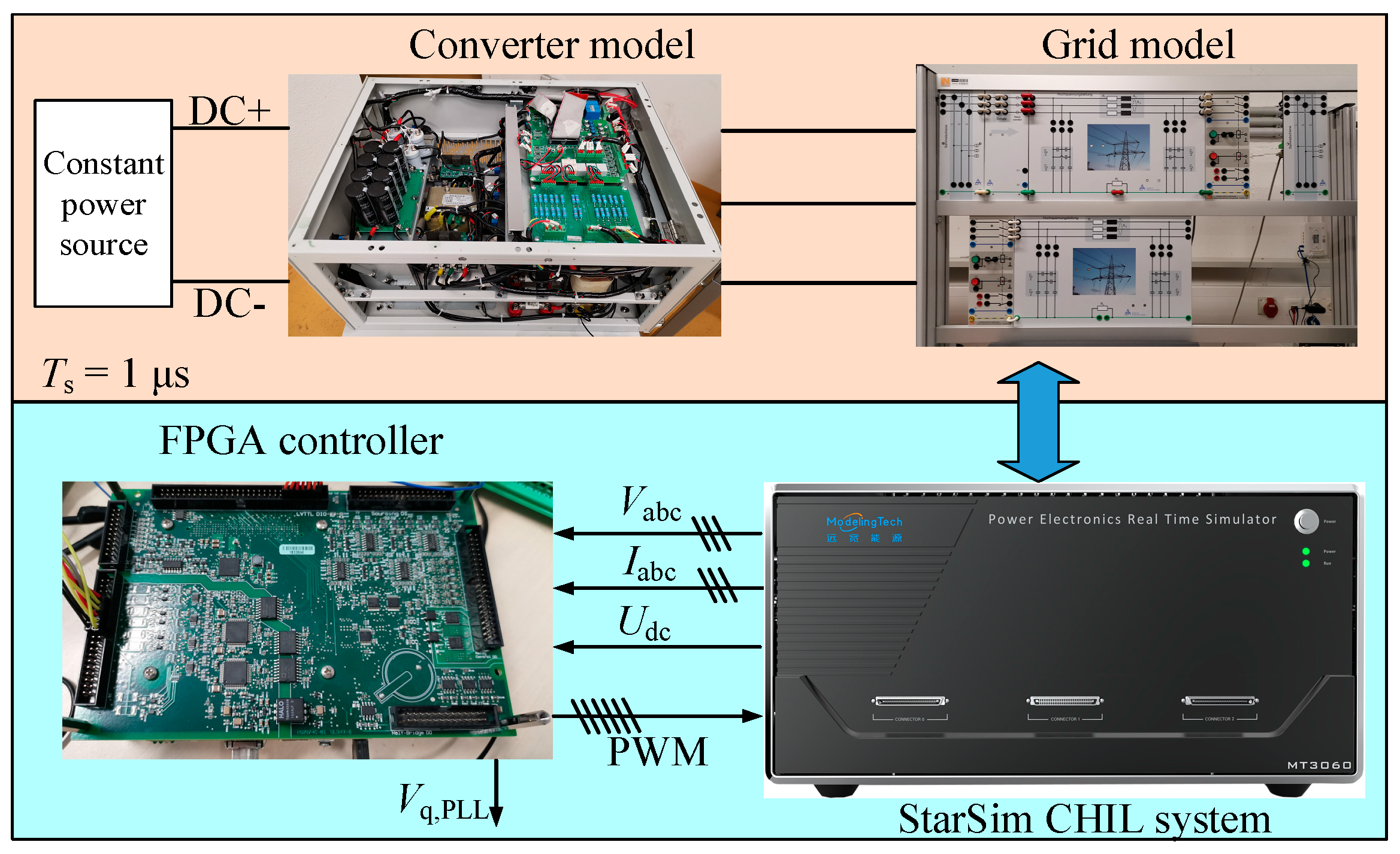Section 5 validates the above findings based on controller hardware-in-the-loop tests. Section 6 concludes the study with a summary of the most important findings.

2. System Modeling

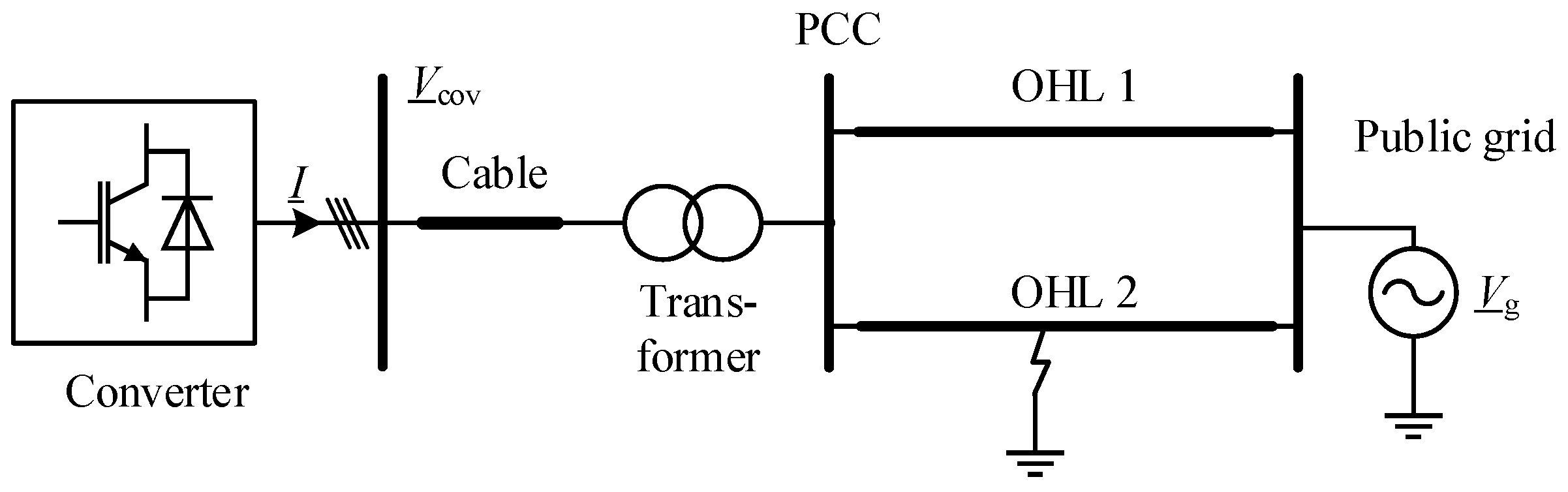
A simple equivalent circuit diagram of a common model of a converter connected to the grid is shown in Figure 1. A three-phase converter is connected to an infinite bus system by a double transmission line (overhead line OHL) [14]. Since the converter must be able to withstand any possible fault, the worst-case situation concerning the stability of a three-phase fault was investigated further.

In Figure 1, the converter is approximated as an ideal current source (I) [14], since the output current tracks the grid voltage’s phase. The expression for the converter terminal’s voltage can be derived as follows:

$${\underset{\_}{V}}_{\mathrm{cov}}=\underset{\_}{Z}\underset{\_}{I}+\underset{\_}{K}{\underset{\_}{V}}_{\mathrm{g}}$$

(1)

where I is the converter’s output current; Z represents the impedance between the converter and the infinite bus system; K can be interpreted as the transfer factor between the grid voltage and converter terminal voltage, and depends on the grid’s topology.

The converter was modeled as an ideal current source, since the control time constants of the outer control loops, such as the PLL, the reactive power control loop and the DC link voltage control loop, are at least one magnitude larger, and thus hardly affect the stability of the inner loop control [20].

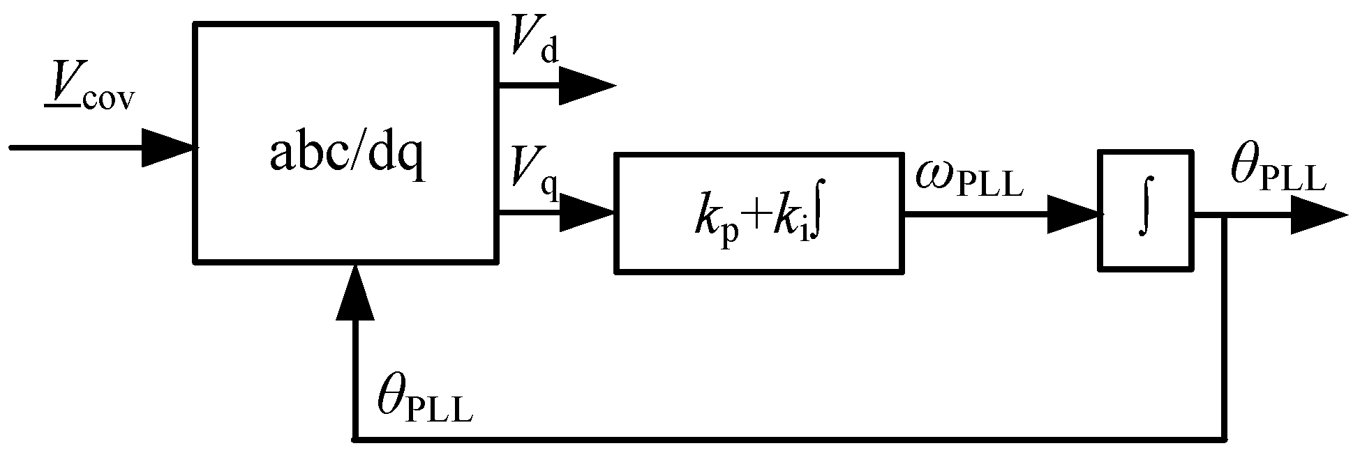
A synchronous reference frame phase-locked loop (SRF PLL) [23] was used to determine the converter terminal voltage’ phase, as shown in Figure 2.

V_cov is converted into its dq-components utilizing Park’s transformation [23]. The PLL uses the q-axis component of the grid voltage V_q as the set point. During steady-state, when the Park’s transformation’s output voltage space vector rotates synchronously with the grid voltage space vector, if V_cov is aligned with the d-component, V_q vanishes.

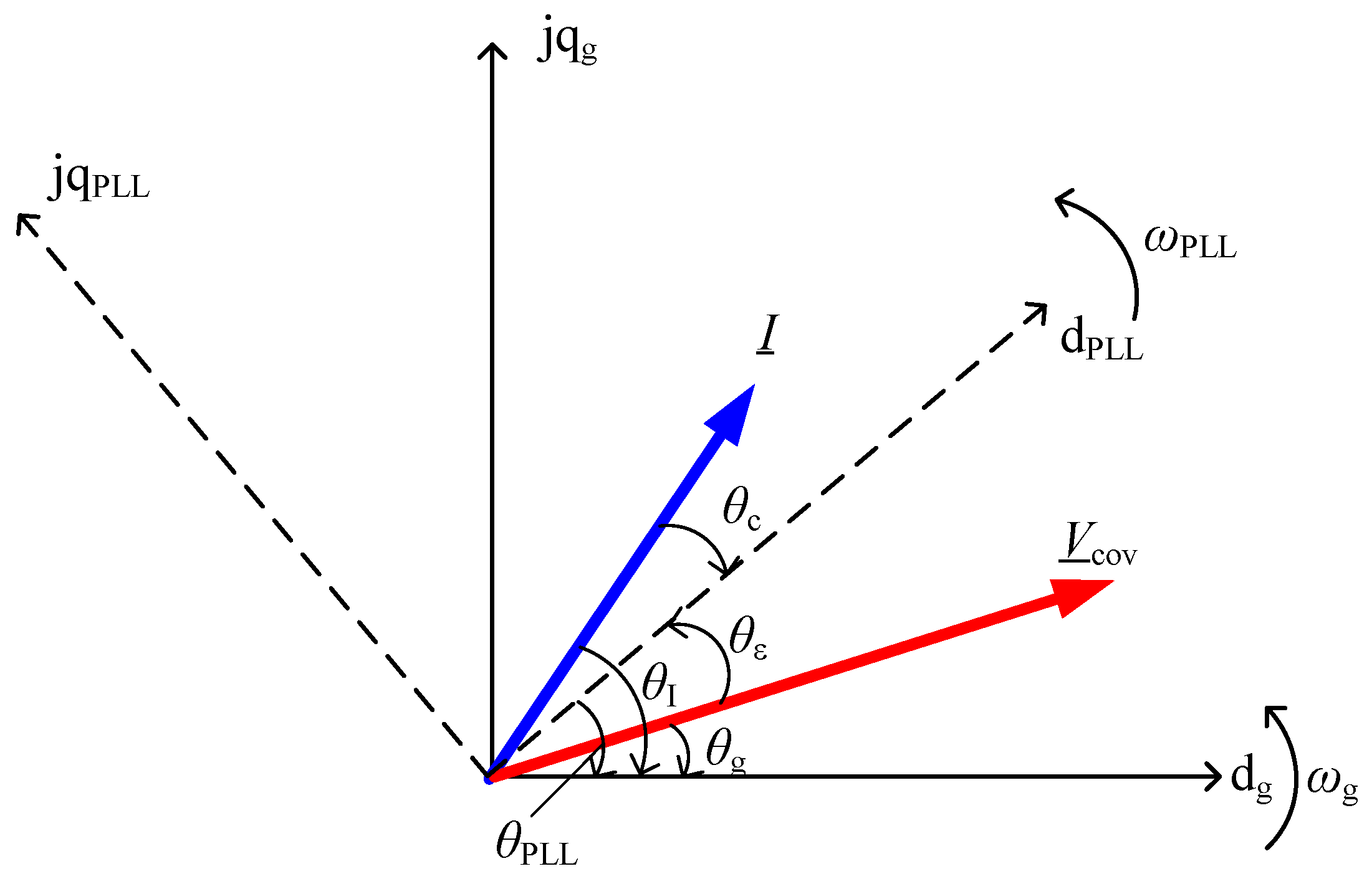
As shown in Figure 3, due to a control deviation of the PLL, the rotating frame of the converter d_PLL-q_PLL (dashed line in Figure 3) and of the grid d_g-q_g (solid line in Figure 3) rotate at different angular velocities, ω_g and ω_PLL.

The PLL’s output is the phase θ_PLL; the grid voltage’s phase V_cov is θ_g. The PLL’s deviation is θ_ε = θ_g − θ_PLL. θ_I is the grid current’s phase and θ_C is the phase of the current reference for the converter’s current control loop.

Assuming that the grid voltage forms a symmetrical three-phase system, the q-axis component of the grid voltage takes the form of [14]:

$$V_{\mathrm{q}}=m_{\mathrm{c}}-m_{\mathrm{g}}\sin \left({\theta }_{\mathrm{PLL}}-{\theta }_{\mathrm{K}}\right),$$

(2)

$$\{\begin{array}{l}{m}_{\mathrm{c}}=\left|\underset{\_}{Z}\right|\left|\underset{\_}{I}\right|\sin \left({\theta }_{\mathrm{Z}}+{\theta }_{\mathrm{C}}\right)\\ m_{\mathrm{g}}=\left|\underset{\_}{K}\right|\left|{\underset{\_}{V}}_{\mathrm{g}}\right|\end{array}.$$

(3)

3. Dynamic Behavior Investigation during and after Fault with Reactive Current Reference

In the investigation of grid faults, the grid states are classified into three stages: pre-fault, during fault, and post-fault. After the faulty line has tripped, the post-fault’s grid impedance changes with respect to the pre-fault’s impedance. However, this change in impedance is much smaller than the difference between the pre-fault’s and fault’s change in impedance. Thus, in this research, the pre-fault’s and post-fault’s grid impedances were assumed to be identical.

This section presents a pseudo-trajectory analysis of a PLL-based converter. In accordance with (2), we first specified the criteria for the existence of an SEP. Then, the criteria were used to derive the relationship between the reactive current reference and PLL stability during a fault.

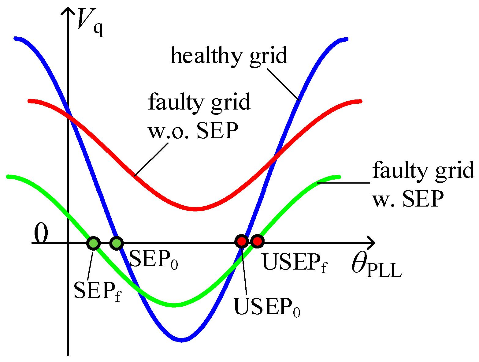
Similar to the classical analysis method of the swing equation widely used in power systems analysis [30], the pseudo-trajectory analysis method can be used for the investigation of the inherent dynamic behavior of the system when the PLL’s control parameters are unknown. According to (2), the trajectory of the systems is illustrated in Figure 4.

In Figure 4, the abscissa and ordinate represent the PLL’s output phase θ_PLL and input V_q of the PLL, respectively. The PLL’s operation point moves along the trajectory (blue, green or red curves in Figure 4). The intersections of the trajectories and the abscissa are the equilibrium points. In Figure 4, two equilibrium points on the blue and green curves exist, with the left one being a stable equilibrium point (SEP₀) and the one at the right representing an unstable equilibrium point (USEP₀) [14]. No equilibrium point exists on the red curve, which implies that the operation point moving along the red curve diverges.

According to (2), when the following occurs:

$$\left|m_{\mathrm{c}}\right|\le m_{\mathrm{g}}$$

(4)

the trajectory has intersection points with the abscissa, i.e., the equilibrium points. The system can converge to its SEP. When (6) is not satisfied, the trajectory has no equilibrium point, and the system diverges.

Applying classical stability analysis to the Jacobian of the system (2) [14] shows that the equilibrium point on the right side of the Figure 4 is a stable equilibrium point (SEP). The left point is an unstable equilibrium point (USEP). The stable equilibrium points’ expression is the following:

$$\mathrm{SEP}={\theta }_{\mathrm{K}}+\arcsin \left(m_{\mathrm{c}}/m_{\mathrm{g}}\right)+2n\mathsf{\pi },n\in \mathbb{Z}$$

(5)

where the n in the (5) implies that the SEP exists periodically [23].

When a fault occurs, criterion (4) may not be satisfied, due to a change in grid impedance as well as a change in |K|, so that the trajectory has no equilibrium point, as depicted in Figure 4’s red curve. The operating point jumps from the original SEP₀ to the red solid line, and then moves continuously to the right in the direction of increasing angle θ_PLL along the red curve.

When criterion (4) is satisfied during a fault, an SEP_f exists, as shown in the green curve in Figure 4. The operating point jumps from the original SEP₀ to the green curve, and then moves during the fault to the left along the green curve to the temporary stable equilibrium point SEP_f. After fault clearing, the operating point jumps from the SEP_f back to the blue curve, and then moves along the blue curve to the original SEP₀.

Further investigation of (5) allows a quantitative stability based on the grid’ parameters and the converter’s active power reference. The expressions for the short-circuit ratio (SCR) of the grid and the converter current are as follows:

$$\{\begin{array}{l}SCR=\frac{{\left|{\underset{\_}{V}}_{\mathrm{g}}\right|}^2}{P_{}^{\ast }\left|\underset{\_}{Z}\right|}\\ \left|\underset{\_}{I}\right|=\frac{P_{}^{\ast }}{\left|{\underset{\_}{V}}_{\mathrm{g}}\right|}\end{array}$$

(6)

where P* is the power reference in per unit.

Substituting (6) into (3) yields the following expression for |m_c|:

$$\left|m_{\mathrm{c}}\right|=\frac{\left|{\underset{\_}{V}}_{\mathrm{g}}\right|}{SCR}\left|\sin \left({\theta }_{\mathrm{Z}}+{\theta }_{\mathrm{C}}\right)\right|$$

(7)

Based on criteria (4) and (3), the critical SCR that stabilizes the PLL can be derived as follows:

$$SCR\ge \frac{1}{\left|\underset{\_}{K}\right|}\left|\sin \left({\theta }_{\mathrm{Z}}+{\theta }_{\mathrm{C}}\right)\right|$$

(8)

When the grid impedance is dominated by its reactance, the impedance’s phase θ_Z is close to π/2, which is the usual condition for transmission grids. If the converter operates at a unity power factor, the current reference’ phase θ_C is 0, so |sin(θ_C + θ_Z)| ≈ 1. In this case, (8) can be further simplified to the following:

$$SCR\ge \frac{1}{\left|\underset{\_}{K}\right|}$$

(9)

|K| is close to 1 in a healthy grid, so the critical SCR in the sense of PLL stability becomes 1. A lower |K| in a faulty grid leads to a higher critical SCR and causes the system to be susceptible to transient instability.

If (10) is met, as follows:

$${\theta }_{\mathrm{C}}=-{\theta }_{\mathrm{Z}}$$

(10)

then |m_c| in (3) constantly equals zero. Therefore, criterion (4) is satisfied for any combination of voltage and grid impedance. In some fault-ride-through strategies [30], (5) can be satisfied by adjusting the phase of the current reference θ_C, which is equivalent to adjusting the ratio of current reference $I_{\mathrm{d}}^{\ast }$ and $I_{\mathrm{q}}^{\ast }$.

During a fault, θ_Z can be obtained by an online estimation algorithm [27,28,29]. In addition, the current reference’s phase can also be controlled adaptively to satisfy (7). For example, V_q or ω_PLL is used as a set point to adjust the θ_C = arctan($I_{\mathrm{q}}^{\ast }$/$I_{\mathrm{d}}^{\ast }$) [5,31]. That is, if $I_{\mathrm{q}}^{\ast }$ = −1.0 p.u. and $I_{\mathrm{d}}^{\ast }$ = 0 p.u., then θ_C = −π/2, which means that the converter delivers the maximum possible reactive power and zero active power into the grid.

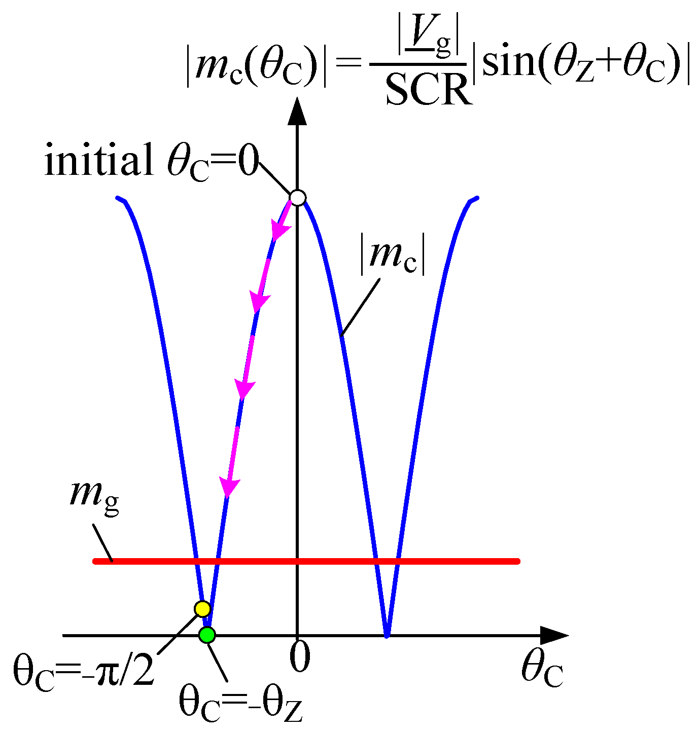
Figure 5 depicts the relationship between the current reference’ phase θ_C and |m_c| and m_g. The abscissa represents θ_C. The blue and red curves represent |m_c| and m_g, respectively. According to criterion (4), |m_c| ≤ m_g, if the operating point lies below the red curve, an SEP exists, e.g., the operating point located at the green point θ_C = −θ_Z or the yellow point θ_C = −π/2. If the operating point moves to the right in the direction of increasing phase, this implies an absorption of reactive power from the grid during the fault. Such behavior of the converter is forbidden during a fault according to grid codes. Therefore, this research only investigated the case in which the operating point moves to the left.

As a fault occurs, the initial operation point is located at the white point, i.e., θ_C = 0. When fault ride-through control [27,28,29,30,31,32,33] is activated, the operation point moves to the left along the blue trajectory with magenta arrows in Figure 5. Neither an online grid impedance estimation algorithm nor an adaptive controller loop can immediately place the operation point in the region m_g, in order to meet criterion (4). Therefore, the SEP’s existence cannot be ensured until θ_C is stabilized, and may even deteriorate the stability performance during this process.

A lower residual voltage implies that the red curve is closer to the abscissa, so a precise fault ride-through control is needed to stabilize the operating point below the red curve as soon as possible, which can be difficult during a fault.

Furthermore, according to grid codes [6], the following are determined:

$$\{\begin{array}{l}{I}_{\mathrm{q}}^{\ast }=k\Delta V_{\mathrm{g}}\begin{array}{cc}& \left|\Delta V_{\mathrm{g}}\right|>0.1 \mathrm{p}.\mathrm{u}.\end{array}\\ I_{\mathrm{q}}^{\ast }=0\begin{array}{cc}\begin{array}{cc}& \end{array}& \end{array} \left|\Delta V_{\mathrm{g}}\right|\le 0.1 \mathrm{p}.\mathrm{u}.\end{array}$$

(11)

in which, ΔV_g is the change in grid voltage and k is the slope of the reactive current, which is often chosen as 2.

When the residual voltage is lower than 0.4 p.u., the converter should inject the maximum reactive current into the grid, i.e., θ_C should be −π/2. However, when adaptive fault ride-through control is activated, the converter injects less reactive current into the grid than required by the grid code in most cases, even if the operating point is at the green point, i.e., θ_C = −θ_Z, due to the resistive part of the grid impedance, θ_Z < π/2.

During a fault, if the grid impedance is dominated by its reactance, then θ_Z approaches π/2, and sin(θ_C + θ_Z) becomes negative and close to zero. This makes |m_c| in the criterion (6) smaller, which will make the system more robust against a loss of stability.

θ_K is close to −π/2 during a fault. If the converter has an SEP due to the injection of reactive currents, the SEP_f is located in the interval (−π/2,0), and lies to the left of the original SEP, as shown in Figure 5.

4. Investigation of Reactive Current Exit Behavior after Fault Clearing

4.1. Reactive Current Exit Behavior

According to grid codes [6,7,8], the requirements for the recovery of reactive and active currents to their pre-fault states after fault clearing are not strictly defined. From the grid operator’s point of view, the converter should reduce its reactive power and boost its active power as soon as possible after fault clearing. However, this is not beneficial for the stability of the converter in all cases, and this phenomenon will be investigated subsequently in this section.

In grid codes [6,7], the reactive and active currents are required to be restored to their pre-fault states within one second. Therefore, manufacturers have developed different reactive current exit strategies.

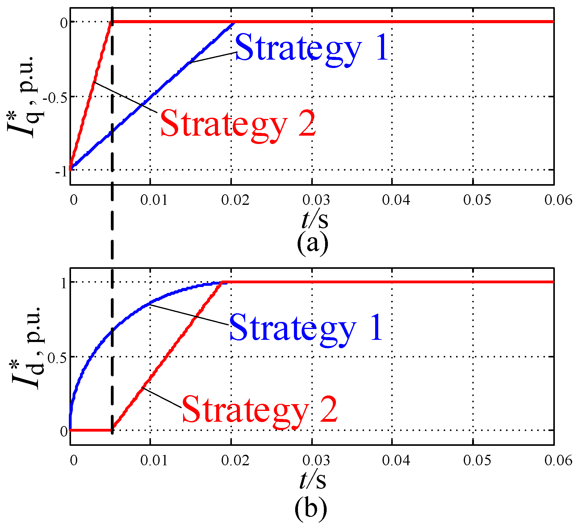
During low residual voltage faults (e.g., |V_g| < 0.4 p.u.), the reactive current reference $I_{\mathrm{q}}^{\ast }$ was set to −I_max, and the active current reference $I_{\mathrm{d}}^{\ast }$ was set to 0, in order to meet requirements of the grid codes, as explained in the previous section. After fault clearing, different strategies exist for returning the reactive current to its pre-fault set point. Upon summarizing our test results from existing commercial converters, we identified two reactive current exit strategies after fault clearing, as shown in Figure 6.

Strategy 1: The reactive current reference $I_{\mathrm{q}}^{\ast }$ changes from −I_max to 0, while the active current reference $I_{\mathrm{d}}^{\ast }$ gradually increases to its pre-fault value. The current references should meet the constraint of (12) to avoid overcurrent [31].

$$I_{\mathrm{d}}^{\ast 2}+I_{\mathrm{q}}^{\ast 2}\le {\left|{\underset{\_}{I}}_{\max }\right|}^2$$

(12)

Strategy 2: In the first stage, the reactive current reference $I_{\mathrm{q}}^{\ast }$ changes from −I_max to 0. The second stage starts after $I_{\mathrm{q}}^{\ast }$ reaches 0, and then the active current reference $I_{\mathrm{d}}^{\ast }$ increases to its pre-fault value.

The curves in Figure 6a are the reactive current references, while the curves in Figure 6b show the active current references. The blue and red curves represent strategy 1 and strategy 2, respectively.

Strategy 1’s reactive current reference is a slope. Constrained by (12), the active current reference is, therefore, not a straight line. In strategy 2, the reactive current reference goes to zero before the active current starts to rise in slope.

The relationship between the actual output current, the current reference and the phase deviation θ_ε is given by the following:

$$\{\begin{array}{l}{I}_{\mathrm{d}}=I_{\mathrm{d}}^{\ast }\cos \left({\theta }_{\mathsf{\epsilon }}+{\theta }_{\mathrm{g}}\right)-I_{\mathrm{q}}^{\ast }\sin \left({\theta }_{\mathsf{\epsilon }}+{\theta }_{\mathrm{g}}\right)\\ I_{\mathrm{q}}=I_{\mathrm{q}}^{\ast }\cos \left({\theta }_{\mathsf{\epsilon }}+{\theta }_{\mathrm{g}}\right)+I_{\mathrm{d}}^{\ast }\sin \left({\theta }_{\mathsf{\epsilon }}+{\theta }_{\mathrm{g}}\right)\end{array},$$

(13)

Correspondingly, the relationship between the actual output power and the phase deviation is given by the following:

$$\{\begin{array}{l}P=-\left|{\underset{\_}{V}}_g\right|I_{\mathrm{q}}^{\ast }\sin \left({\theta }_{\mathsf{\epsilon }}\right)+\left|{\underset{\_}{V}}_g\right|I_{\mathrm{d}}^{\ast }\cos \left({\theta }_{\mathsf{\epsilon }}\right)\\ Q=-\left|{\underset{\_}{V}}_g\right|I_{\mathrm{d}}^{\ast }\sin \left({\theta }_{\mathsf{\epsilon }}\right)-\left|{\underset{\_}{V}}_g\right|I_{\mathrm{q}}^{\ast }\cos \left({\theta }_{\mathsf{\epsilon }}\right)\end{array},$$

(14)

If the phase deviation θ_ε ≠ 0, the actual output current does not match the calculated output current in the controller; therefore, the actual output power does not match the controller’s setting.

If $I_{\mathrm{q}}^{\ast }$ = −I_max and $I_{\mathrm{d}}^{\ast }$ = 0 when the fault is cleared and the phase deviation at this time instant is denoted by θ_ε, then the actual output active power is given by the following:

$$P=-\left|{\underset{\_}{V}}_g\right|\left|I_{\max }\right|\sin \left({\theta }_{\mathsf{\epsilon }}\right),$$

(15)

That is, if the operating point is located left of the SEP (θ_ε < 0), then the actual output active power is negative. The converter draws power from the grid and transfers it into its DC link. If the phase deviation θ_ε is π/2, then the actual output power of the converter is −|V_g||I_max|, i.e., the maximum output power that the converter will backfill from the grid to the converter’s DC Link.

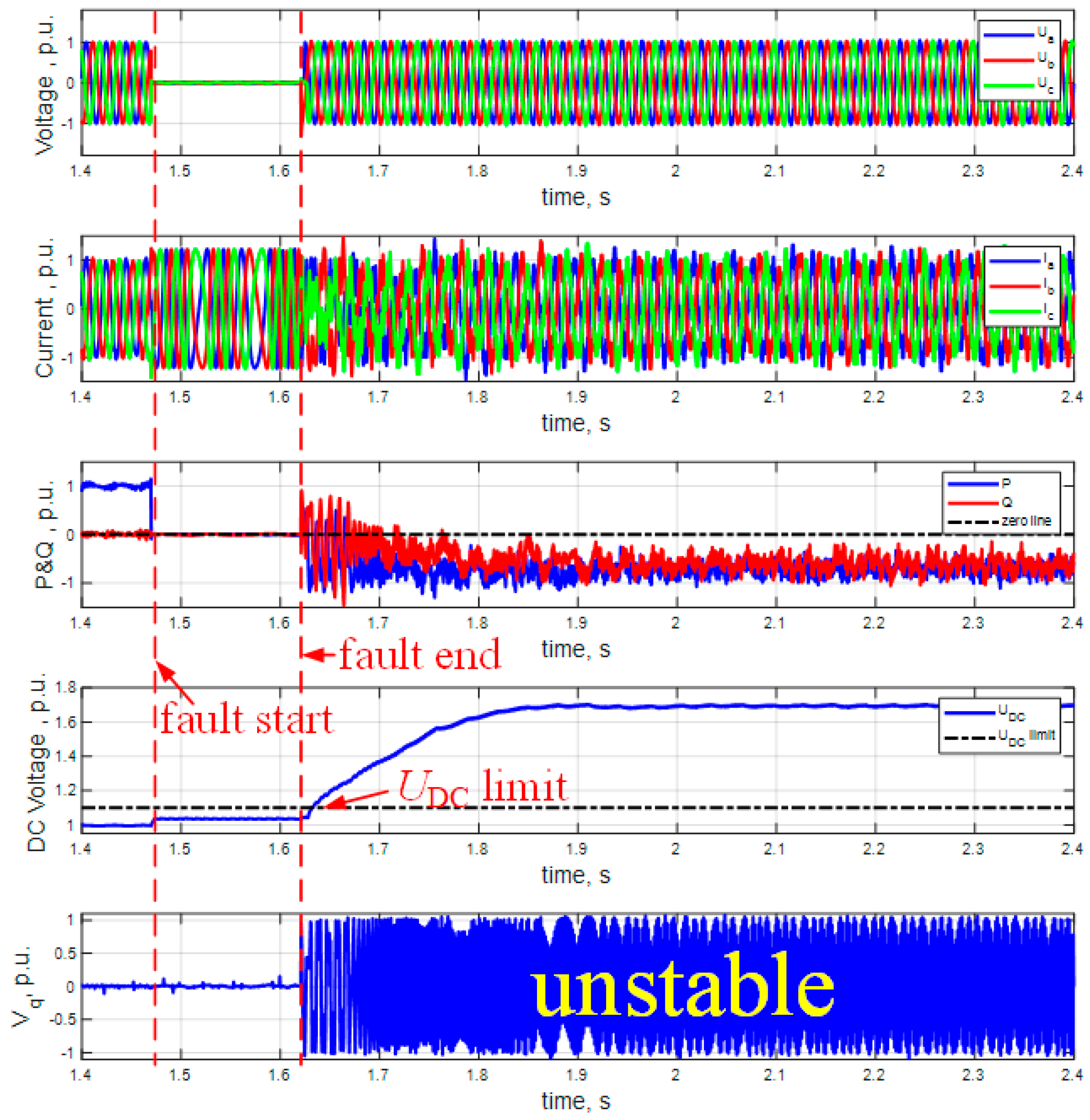
After a fault occurs, the low grid voltage limits the active power output. The DC link’s power balance cannot be met. Thus, the surplus energy is injected into the DC capacitor and causes the DC link voltage to rise [14]. In order to keep the DC link voltage below a specific threshold, the chopper circuit is activated to absorb the excess energy. After fault clearing, if the output active power is negative, the chopper resistor, which is designed for the converter’s rated power, may be unable to further absorb the active power from both the source and the grid side. This results in the DC link voltage crossing its upper limit, and so triggering the protection and initiating the converter’s tripping. This behavior has to be avoided under all fault situations.

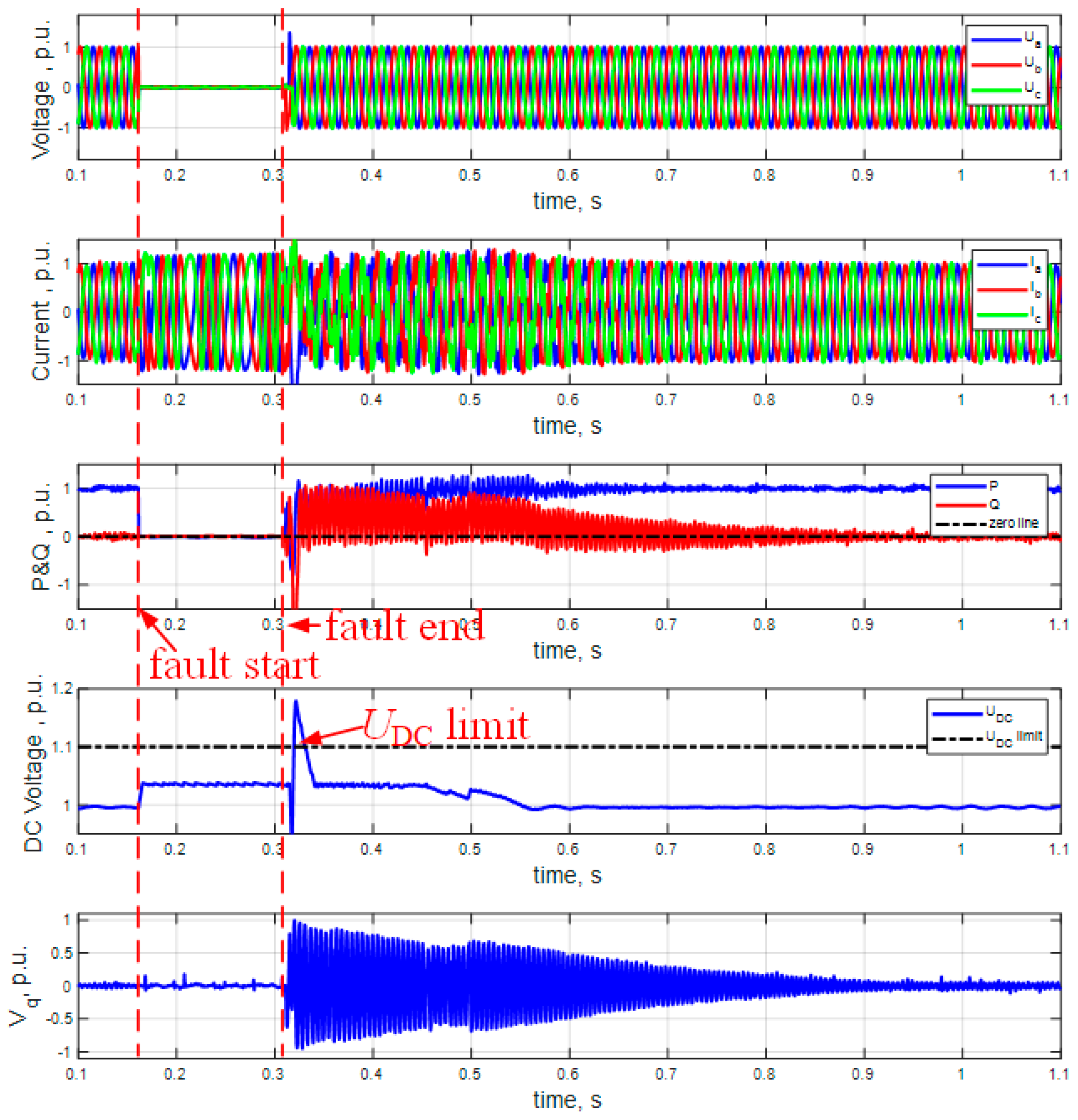
The reduction in $I_{\mathrm{q}}^{\ast }$ after fault clearing and the reduction in θ_ε due to the stabilization of the PLL allows the actual output power to be finally stabilized at a value that is consistent with the DC link’s power balance. However, the PLL’s dynamics and the different strategies of $I_{\mathrm{d}}^{\ast }$ reduction lead to a complex dynamic process of the converter at the post-fault stage. The power may oscillate between positive and negative output, thus jeopardizing the stability of the converter, and even the grid’s operation.

In summary, a reactive current exit strategy should meet the following three requirements:

• Reduces negative active power magnitude;
• Reduces power oscillations;
• Increases active power as soon as possible while satisfying 1 and 2.

In the time-domain simulation presented in this section, the control parameters of the phase-locked loop were K_pPLL = 0.32, K_iPLL = 0.32 1/s. The rate of reactive current exit used in the simulation was 5 p.u./s.

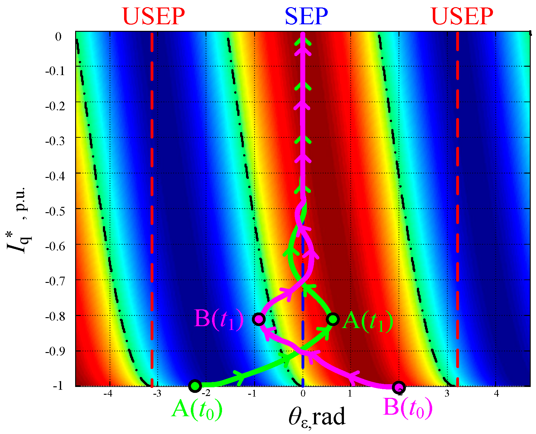
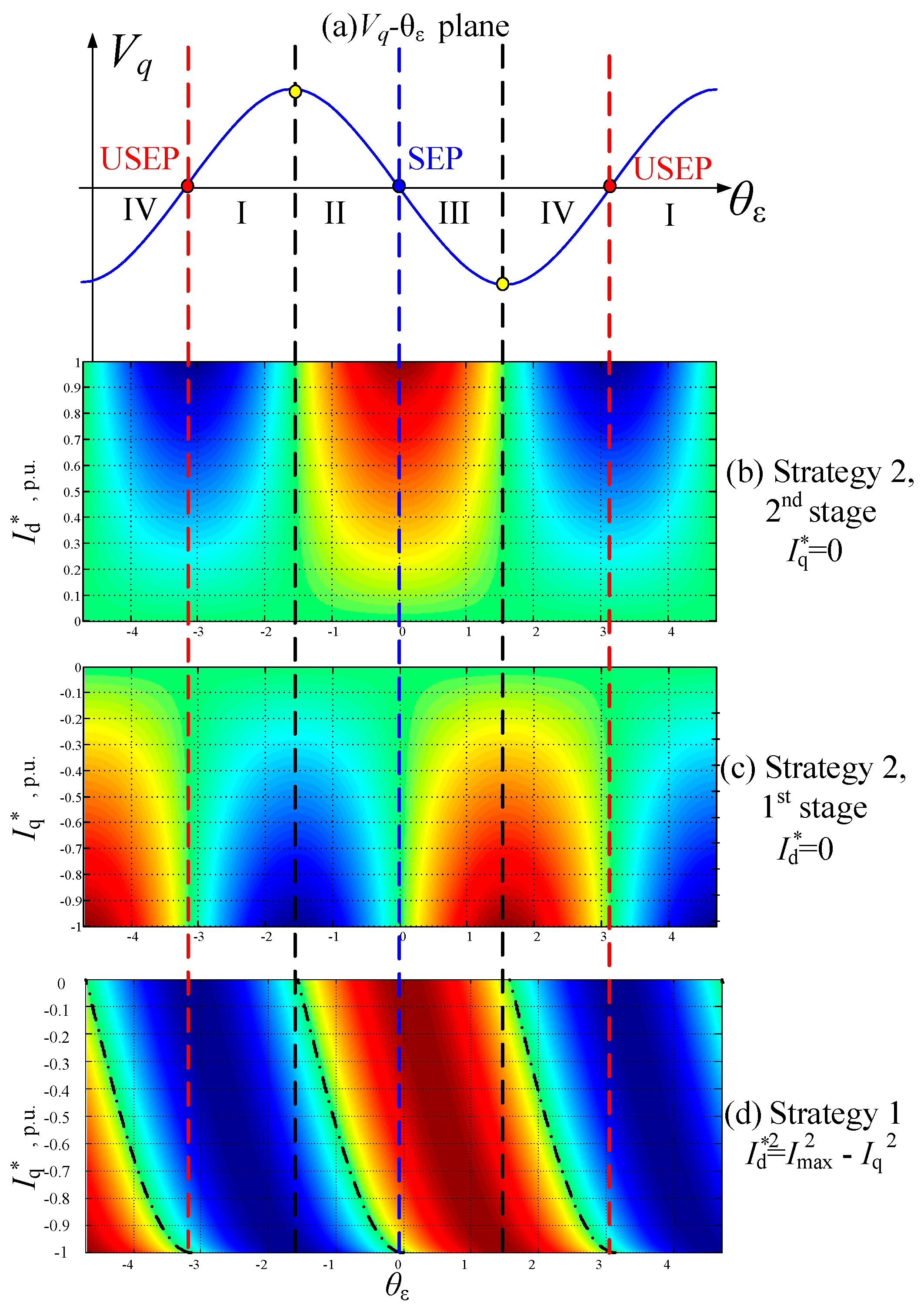
Figure 7 shows how the actual output active power was affected by the phase deviation θ_ε for a reactive current reference. The abscissa represents the phase deviation between the converter frame and grid frame; the ordinate is the reactive current reference, and the colors represent the actual output active power. As the active power approached 1.0 p.u., the area’s color turned closer to dark red. As the active power approached −1.0 p.u., there existed an active power flow from the grid into the converter, and the area’s color turned closer to dark blue. The black dashed lines denote the boundaries between positive and negative active power. The following example serves as further explanation.

Based on (14), the expressions for the boundaries of positive and negative active power are the following:

$$\{\begin{array}{l}P\le 0,\begin{array}{cc}& \end{array}\arctan \left(I_{\mathrm{d}}^{\ast }/I_{\mathrm{q}}^{\ast }\right)\le {\theta }_{\mathsf{\epsilon }}\le \arctan \left(I_{\mathrm{d}}^{\ast }/I_{\mathrm{q}}^{\ast }\right)+n\mathsf{\pi }\\ P>0,\begin{array}{cc}& \end{array}\arctan \left(I_{\mathrm{d}}^{\ast }/I_{\mathrm{q}}^{\ast }\right)-n\mathsf{\pi }<{\theta }_{\mathsf{\epsilon }}<\arctan \left(I_{\mathrm{d}}^{\ast }/I_{\mathrm{q}}^{\ast }\right)\end{array},$$

(16)

in which n ∈ $\mathbb{Z}$.

The position of the initial point after a fault depends on the fault duration and the phase trajectory dynamics of the operating point during the fault. Here, two arbitrary post-fault initial points, A(t₀) and B(t₀), were located to the left and right of the SEP, respectively, in Figure 7. The two trajectories depicted in green and magenta show the course of the phase deviation with increasing time as a function of the reference value of I^*. It was noted that the initial point was defined by the fault configuration as well as the fault time, and could only slightly be influenced by converter control during a no SEP fault. After fault clearing, the PLL rapidly reduced the phase deviation, while A and B moved closer to the SEP. A and B experienced an overshoot after passing the SEP. At t₁, the phase deviations of A and B reached their respective maxima after passing the SEP.

As |$I_{\mathrm{q}}^{\ast }$| decreased, point A moved from the dark blue region towards the light blue as well as the red regions, i.e., the actual output power changed from negative to positive at t₁, whereas B moved from the dark red area to the blue area, i.e., the actual output power changed from positive to negative.

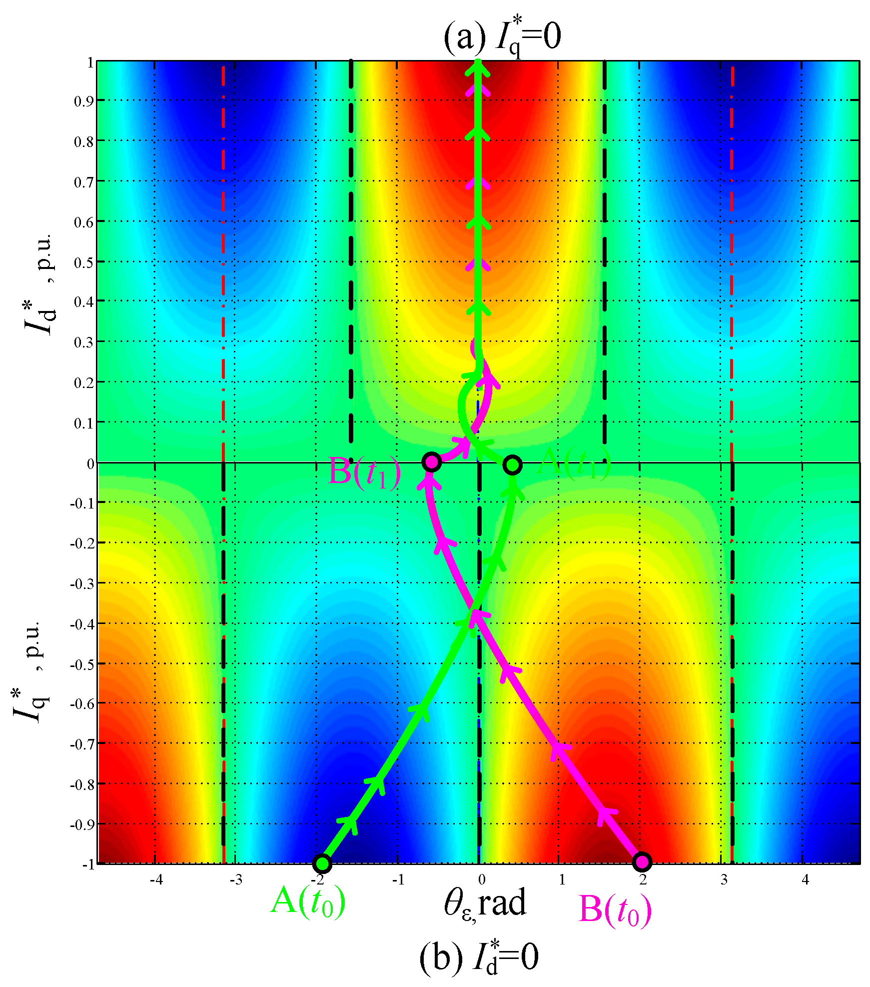
Figure 8 presents the actual output active power, as affected by the phase deviation θ_ε for the reactive current reference of strategy 2. Figure 8b illustrates the heat map of strategy 2’s first stage (t₀ < t < t₁), with $I_{\mathrm{d}}^{\ast }$ = 0 and the active power varying with $I_{\mathrm{q}}^{\ast }$ and the PLL’s phase deviation. Figure 8a shows the heat map of strategy 2’s second stage (t > t₁), with $I_{\mathrm{q}}^{\ast }$ = 0 and the active power varying with the phase deviation and $I_{\mathrm{d}}^{\ast }$.

Based on (14), the boundaries’ expressions of positive and negative active power of strategy 2’s first stage (t₀ < t < t₁) and second stage (t > t₁) in Figure 8 are as follows:

$$\{\begin{array}{l}P>0,\begin{array}{cc}& \end{array}0+2n\mathsf{\pi }<{\theta }_{\mathsf{\epsilon }}<\mathsf{\pi }+2n\mathsf{\pi }\\ P<0,\begin{array}{cc}& \end{array}-\frac{\mathsf{\pi }}{2}+2n\mathsf{\pi }<{\theta }_{\mathsf{\epsilon }}<\frac{\mathsf{\pi }}{2}+2n\mathsf{\pi }\end{array},$$

(17)

In Figure 8b, |$I_{\mathrm{q}}^{\ast }$| rapidly went to zero in the first stage. A and B overshot after passing the SEP. At t₁, the |$I_{\mathrm{q}}^{\ast }$| corresponding to points A and B were zero, and then entered the second stage: the $I_{\mathrm{d}}^{\ast }$ gradually increased, as shown in Figure 8a.

Due to the different positions of the initial points, A and B had different output active power in the first stage, as depicted in Figure 8b. In the second stage, the actual power outputs of A and B were always positive after the second stage, and continued to grow towards the set value, as illustrated in Figure 8a.

Due to the dynamics of $I_{\mathrm{q}}^{\ast }$ and the PLL’s phase deviation, the actual active power output experienced oscillations between positive and negative values, since the trajectories passed the dashed black power limit lines several times. The oscillations in active power compromised the stability of the converter and power system. The active power oscillations could be suppressed by adjusting the current reference and phase deviation.

4.2. Adjustment Strategy for the Current Reference after Fault Clearing

The above investigations show that the initial phase deviation after fault clearing has a strong influence on the active power. In order to improve the active power’s dynamics, the initial phase deviations after fault clearing were classified into four areas in one cycle of V_q (θ_ε), as illustrated in Figure 9.

In order to determine the phase deviation θ_ε, i.e., the position of the initial point after a fault in Figure 7 or Figure 8, this research used V_q and dV_q/dt to determine the area where its phase deviation θε is located, as presented in Figure 9a.

Area I is located between the left USEP and V_q’s maximum. When the initial phase deviation was located in area I, with strategy 1 (Figure 9d), during the approach to the SEP, the operating point passed through the dark blue region, i.e., the negative maximum active power, regardless of how the curve of $I_{\mathrm{q}}^{\ast }$ was changed. If strategy 2 (Figure 9c) was used, at strategy 2’s first stage, it was possible to keep the operating point in the light green or light blue region most of the time as it approached the SEP, i.e., the active power being close to 0. At strategy 2’s second stage, after $I_{\mathrm{q}}^{\ast }$ went to zero, raising $I_{\mathrm{d}}^{\ast }$, as provided in Figure 9b, allowed the output active power to remain at a small negative value, or always positive, as the operating point approached the SEP.

Area II locates between V_q’s maximum and the SEP. According to the investigations in Section 3, the SEP_f during the fault was in this area. Therefore, this area was the most likely area for initial phase deviation after fault clearing. Using either strategy 1 (Figure 9d) or strategy 2 (Figure 9c) caused the operating point to pass through the dark blue region, regardless of how the $I_{\mathrm{q}}^{\ast }$ was changed. However, a rapid reduction in $I_{\mathrm{q}}^{\ast }$ minimized the duration of the blue region.

Area III locates between the SEP and V_q’s minimum. With strategy 1 or strategy 2, the operating point was always in the red area, i.e., the converter always delivered active power into the grid. This allowed the DC link voltage to stabilize quickly after fault clearing.

Area IV locates between the V_q’s minimum and the right USEP. With strategy 1, the operating point could pass through the blue and red areas as it approached the SEP, i.e., a rapid oscillation of the active power from positive to negative. With strategy 2, the operating point was always in the red or light green area as it approached the SEP, i.e., the active power was always positive, or to a lesser negative value.

The converter could use V_q and d V_q/dt to determine the area where the operating point was located, as shown in

Table 1. Adjustment strategy for the current reference after fault clearing.

Area	Vq	dVq/dt	${\mathit{I}}_{\mathbf{q}}^{\mathbf{*}}$	${\mathit{I}}_{\mathbf{d}}^{\mathbf{*}}$
I	≥0	≥0	Rapidly decreasing	Increase after Vq ≈ 0
II	≥0	<0	Rapidly decreasing	$I_{\mathrm{d}}^{\ast 2}={\left|I_{\max }\right|}^2-I_{\mathrm{q}}^{\ast 2}$
III	<0	≥0	Rapidly decreasing	$I_{\mathrm{d}}^{\ast 2}={\left|I_{\max }\right|}^2-I_{\mathrm{q}}^{\ast 2}$
IV	<0	<0	Rapidly decreasing	Increase after Vq ≈ 0

. This information could be used to adjust the current reference dynamically.

In addition, enhancing the PLL’s dynamics can also improve the behavior in a way to more rapidly reduce the phase deviation. This can also dampen the oscillations of the output power more efficiently. The actual active power can be controlled as desired, regardless of the area in which the initial phase deviation lies, if the operating point can be stabilized rapidly at the SEP, as shown in Figure 7 and Figure 8, and with (14).

The literature [23] proposes that temporarily increasing the PLL’s cut-off frequency after fault clearance, while guaranteeing small-signal stability, can expand the domain of attraction, and also accelerate the PLL’s recovery to stability.

5. Experimental Verification

5.1. Experimental Setup

In this section, the investigation results and the improvements from the above section were validated through a controller hardware-in-the-loop (CHIL) test [14,23]. When a real converter encounters a dramatically changing grid, a loss of synchronization can easily lead to an overcurrent or overvoltage, and activate its hardware protection, resulting in tripping. Deactivating the hardware protection in order to investigate the full failure process can jeopardize the converter’s hardware. Performing CHIL tests on the controller can avoid damaging the hardware, while investigating the full failure process during and after a fault. In this study, the controller hardware-in-the-loop test setup is shown in Figure 10.

In the test setup, the hardware part of the converter under test as well as the grid model are shown in Figure 1. They were simulated in real-time with a 1 μs time step in Starsim CHIL’s control hardware-in-the-loop system. A Xilinx Zynq-7020 FPGA-based converter controller acquired the grid voltage, output current and DC link voltage signals from the CHIL system, and controlled the IGBTs and the chopper circuit in the CHIL system.

In the CHIL test, the parameters of the 10 kW converter were as follows: the filter inductance was 9.6 mH, the filter capacitance was 10 μF, the DC link capacitance was 1600 μF, and the chopper resistance was 58 Ω. The control parameters in the FPGA were as follows: current control parameter K_pc = 5, K_ic = 300 1/s, DC control parameter K_pdc = 0.1, K_idc = 100 1/s, and phase-locked loop control parameters K_pPLL = 0.32, K_iPLL = 0.32 1/s. The upper limit of current amplitude was 1.2 p.u. The grid side voltage was 400 V, SCR was 5, and the X/R ratio was 7. The reactive current exit strategy 1 in Figure 6 was used to improve the recovery rate of output active power.

5.2. Inject Reactive Current to Improve the Stability Performance of the PLL

Table 2. Test cases.

Figure	Residual Voltage	Rate of Reactive Current Reduction	Variable PLL Parameter
Figure 11	0.05	No reactive current injection	No
Figure 12	0.05	80 p.u./s	No
Figure 13	0.47	5 p.u./s	No
Figure 14	0.47	80 p.u./s	No
Figure 15	0.47	5 p.u./s	Yes

shows the test cases used in the experiments and the figure numbers of the test results.

In the experimental results in Figure 11 and Figure 12, the fault impedance was set to result in a residual voltage of 0.05 p.u. and a fault duration of 150 ms.

In Figure 11, the grid voltage was reduced to approximately 0.05 p.u. after the fault occurred. During the fault, the converter was configured to not inject reactive current into the grid. Since there was no SEP in the system during the fault, the PLL’s operating point moved continuously away from the original SEP. This resulted in rapid oscillations in the current’s frequency and phase, as well as small oscillations in V_q. At the moment of fault clearing, the operating point lay outside of the domain of attraction, so the system diverged and V_q oscillated continuously. The active power (blue curve) oscillated due to the loss of synchronization, causing the converter to inject power from the grid into the DC link, resulting in a peak in the DC link voltage. A converter will stop operation after a rapidly increasing DC link voltage, since the hardware protection is triggered.

In Figure 12, the converter was configured to inject reactive current into the grid at 10 ms after the fault. The operating point tended to converge to the new SEP during the fault, so its operating range in the phase plane was bounded. After fault clearing, the operating point should lie within the domain of attraction, so the operating point converged after the oscillation. The system was able to restore stability. As shown in Figure 12, V_q converged to 0 after the oscillation, and the active power (blue curve) oscillations were properly damped and stabilized at 1.0 p.u. At the moment of fault clearing, the initial phase deviation and the reactive current reference led to a negative active power peak, which caused the DC link voltage to rise rapidly.

Experiments on the effect of the reactive current exit strategy on the converter were carried out below.

5.3. Fast Reactive Current Exit Strategy

In the results of Figure 13 and Figure 14, the fault impedance was set to result in a residual voltage of about 0.47 p.u. and a fault duration of 150 ms. The rates of reactive current reduction in the experiments of Figure 13 and Figure 14 were 5 p.u./s and 80 p.u./s, respectively.

In Figure 13, 10 ms after the fault, the converter injected a reactive current of 1.2 p.u. into the grid, and the reactive power (red curve) was about 0.5 p.u. during the fault, while the active power dropped to 0. After fault clearing, the magnitude as well as the duration of the negative active power were larger, resulting in a larger energy feedback from the grid to the DC link, which caused the DC link voltage to surge to 1.15 p.u. Although the chopper circuit was activated, it could not reduce the DC link voltage. This triggered a hardware protection of the converter.

5.4. Fast Reactive Current Exit Strategy but Not Fast System Stabilization

In Figure 14, after fault clearing, the peaks in the negative active power were very small in magnitude as well as duration, due to the very fast reduction in $I_{\mathrm{q}}^{\ast }$, resulting in a very small amount of energy feedback from the grid into the DC link. Therefore, the peaks in the DC link voltage were not significant after the fault clearing.

In Figure 14, after fault clearing, $I_{\mathrm{q}}^{\ast }$ decreased rapidly, while the $I_{\mathrm{d}}^{\ast }$ rose rapidly. However, since the phase-locked loop was still oscillating after fault clearing, the actual active and reactive currents did not quickly track their commands, due to the output angle’s deviation. The reactive and active power oscillated around the desired value, resulting in the converter not being able to quickly increase the active power output.

5.5. Variable PLL Parameters Will Speed up System Stabilization

In the experimental results in Figure 15, the fault impedance was set to cause a residual voltage of about 0.47 p.u. and a fault duration of 150 ms. The reactive current reduction rates were 5 p.u./s, which was the same setup as in Figure 13. After fault clearing, the dynamic performance of the phase-locked loop was temporarily boosted to allow the operating point to converge quickly near the SEP, and then the dynamic performance of the loop was restored to its original values.

After the fault clearing, the fluctuations in V_q were very small, and then immediately stabilized at 0. Comparing Figure 13 with Figure 15, the active and reactive power curves (red and blue curves) are smooth, and do not show pronounced oscillations, and are able to decrease or increase at the desired rate. Thus, there were no obvious peaks in the DC link voltage either.

Therefore, it was verified that the dynamical setting of the PLL parameters led to improved transient stability behavior; thus, a proper setting of these parameters can avoid a tripping of the converter in the case of severe grid faults.

6. Conclusions

In this study, a grid-side converter connected to a power system via double transmission lines was modeled by employing large-signal models.

Based on the mathematical description of this model, this study investigated the fault dynamics of the converter-grid system and obtained a stability criterion. It was derived and verified that during a severe grid fault, the injection of reactive current into the grid enhanced the stability of the converter’s phase-locked loop circuit, and thus improved the stable performance of the whole converter system during the fault. The study also investigated the exit strategy of a reactive current after fault clearing. Due to phase deviations from a phase-locked loop, reactive current may cause the converter to backfill power from the grid to the DC link; the power balance of the DC then becomes unbalanced, and can lead to tripping the converter due to DC link voltage limitations. To address this phenomenon, various exit strategies for reactive current were proposed. The strategies used in this study were to increase the active current reference while quickly reducing the reactive current reference value after fault clearing. The control time constant of the PLL was also increased instantaneously after the fault, in order to expand the DOA and speed up the PLL’s convergence. Finally, the role of reactive currents during the fault and different exit strategies of the reactive current were verified in the controller hardware-in-the-loop tests.