A WGAN-GP-Based Scenarios Generation Method for Wind and Solar Power Complementary Study

Abstract

The issue of renewable energy curtailment poses a crucial challenge to its effective utilization. To address this challenge, mitigating the impact of the intermittency and volatility of wind and solar energy is essential. In this context, this paper employs scenario analysis to examine the complementary features of wind and solar hybrid systems. Firstly, the study defines two types of complementary indicators that distinguish between output smoothing and source-load matching. Secondly, a novel method for generating wind and solar output scenarios based on improved Generative Adversarial Networks is presented and compared against the conventional Monte Carlo and Copula function methods. Lastly, the generated wind and solar scenarios are employed to furnish complementary features. The testing results across eight regions indicate the proposed scenario generation method proficiently depicts the historical relevance as well as future uncertainties. This study found that compared to the Copula function method, the root mean square error of the generated data was reduced by 4% and 3.4% for independent and hybrid systems, respectively. Moreover, combining these two resources in most regions showed that the total output smoothness and source-load matching level cannot be enhanced simultaneously. This research will serve as a valuable point of reference for planning and optimizing hybrid systems in China.

1. Introduction

With the global environmental pollution and energy crisis, variable renewable energy (VRE), such as solar and wind power, plays an increasingly important role in energy production [1,2,3,4]. Development and utilization of wind and solar energy is not just an alternative traditional energy resource, but also an obligation and urgent necessity in order to achieve sustainable development [5]. However, the output power of VRE is usually strongly fluctuant due to the intermittency and volatility of solar and wind energy. As a result, large-scale solar and wind energy integration would bring new challenges to the power grid [6,7]. The accommodation problem is particularly prominent, and wind and solar curtailment occasionally occur. Taking Qinghai Province in China as an example, the wind and solar curtailment ratio in 2021 reached 10.7% and 13.8%, respectively, far exceeding the national average level. This problem can be partially overcome by utilizing wind and solar power’s synergy and complementary characteristics on different temporal and spatial scales. Research in other locations shows that the combination of wind and solar energy could improve the stability of power systems. Therefore, it is essential to study the complementary attributes of VRE to enhance the system’s ability to peak shaving and valley filling [8,9].

In the past, the correlation study of two variables mainly focused on calculating the correlation coefficient between random variables directly to reflect the degree of their correlation [10].

Table 1. Details of complementary study.

Article	Location	Data Resolution	Correlation Coefficient
Cantão et al. [13]	Brazil	Hourly, monthly	Pearson, Spearman
Kapica et al. [14]	global	Daily	Kendall
Couto et al. [15]	Portugal	Hourly, daily	Pearson, capacity factor
Frank et al. [16]	European countries	Daily	Pearson
Lv et al. [17]	China	Daily	Spearman
Dirk et al. [18]	Germany	Daily, seasonal	Kendall
Hoicka et al. [19]	Canada	Hourly	Kendall
Jurasz et al. [20]	Poland	15-min, hourly	Capacity factor
Sterl et al. [21]	Africa	Hourly	Proposed one index
Prasad et al. [22]	Australia	Hourly	Proposed two indexes
Bett et al. [23]	the United Kingdom	6-hourly, Daily	Pearson
Shaner et al. [24]	the United States	Hourly	Kendall
Costoya et al. [25]	North America	Hourly	Proposed two indexes

shows the details of the correlation study of wind and solar in different studies. The time-domain energy complementarity between wind and solar energy has been assessed in many sites, and correlation coefficients such as Pearson, Kendall, and Spearman are the most commonly used indexes in quantifying and evaluating the complementary properties between wind and solar power. It is easy and convenient to calculate the correlation coefficient directly, but there are drawbacks to this approach. For instance, the most commonly used Pearson correlation coefficient only reflects the linear relation [11]. Furthermore, the correlation coefficient still needs to be further justified from a physical or mathematical viewpoint [12]. The copula method is often applied to avoid this situation. It is used as a link function of the marginal cumulative distribution functions of the wind speed and the radiation intensity. The Kendal correlation coefficient is indirectly calculated to describe the correlation. Xu et al. combined the Copula and Gaussian kernel functions to establish a dependency model for wind and solar energy. They applied the resulting Kendall correlation coefficient for wind and solar complementary research [11].

The scenario generation approach can effectively express the randomness and interdependence of VREs output [26]. The method is also developed to estimate how large-scale wind and solar energy productions could be potentially involved to complement each other. The scenario approach can be considered as generating a variety of time trajectories that can represent inherent stochastic characteristics. Currently, the most commonly used scenario-generation methods are based on statistical models. Firstly, to fit a probability model from historical data, it is sampled to generate new scenarios [27,28], such as the Monte Carlo method (MC) [29], the Copula function method (Copula), etc. [30,31,32]. At the same time, these methods typically assume that the VRE output meets a particular probability distribution. Monforti et al. used the MC random sampling method to study the complementary characteristics of wind and solar resources [33]. Additionally, unsupervised learning methods such as the machine learning clustering method [10] and principal component analysis method [34] can also generate typical scenarios to capture the correlation between solar and wind power. Zhang et al. used the principal component analysis method to evaluate the complementary effects of wind and solar energy [35]. However, the uncertainty of VRE output encompasses complex temporal-spatial and meteorological correlations [36], and there may be some unknown correlations. It is difficult for shallow algorithms to fully exploit the information and features contained in the output data.

Compared with traditional algorithms, data-driven deep learning methods can mine the high-dimensional nonlinear characteristics of historical data, thereby improving the accuracy of the description of VRE uncertainty characterizations. Chen et al. generated the wind and solar output scenarios by using Generative Adversarial Networks (GAN) [37], and Zhang et al. generated the amount of wind resource output by using the Wasserstein GAN-Gradient Penalty (WGAN-GP) [38]. Zhu et al. generated single-location and multi-location scenarios for wind power by using the WGAN-GP [39]. Tang et al. generated scenarios for newly built wind farm by using the RAC-GAN [40]. However, the method of scenario generation based on deep learning is mainly applied in power system scheduling analysis, and there are few studies on the correlation of wind and solar output to the best of our knowledge.

In summary, the relevant researchers have conducted meaningful research on wind and solar power systems and achieved some significant results. However, the following two aspects remain to be addressed:

• In complementary characteristics of VRE research, most studies only focus on the complementary performance of wind and solar resources, while the matching degree of the combined output to the load is usually ignored. Moreover, the impact of the volatility of VRE output itself is overlooked by correlation coefficients, which only pay attention to the wholeness of data.
• The traditional probabilistic model does not fully consider wind and solar resources’ historical and unknown relationship. In addition, these methods require a prior assumption that the data obeys a specific probability distribution, such as a Weibull distribution, Beta distribution, etc. However, the actual environment is complex, and the assumed distribution may not fit the real condition. On the other hand, existing research based on deep learning lacks relevant research on the complementary properties of new energy sources.

Taking the eight regions of Haixi, Qinghai province, as examples, contributions to solve the above problems in this paper are concluded as follows:

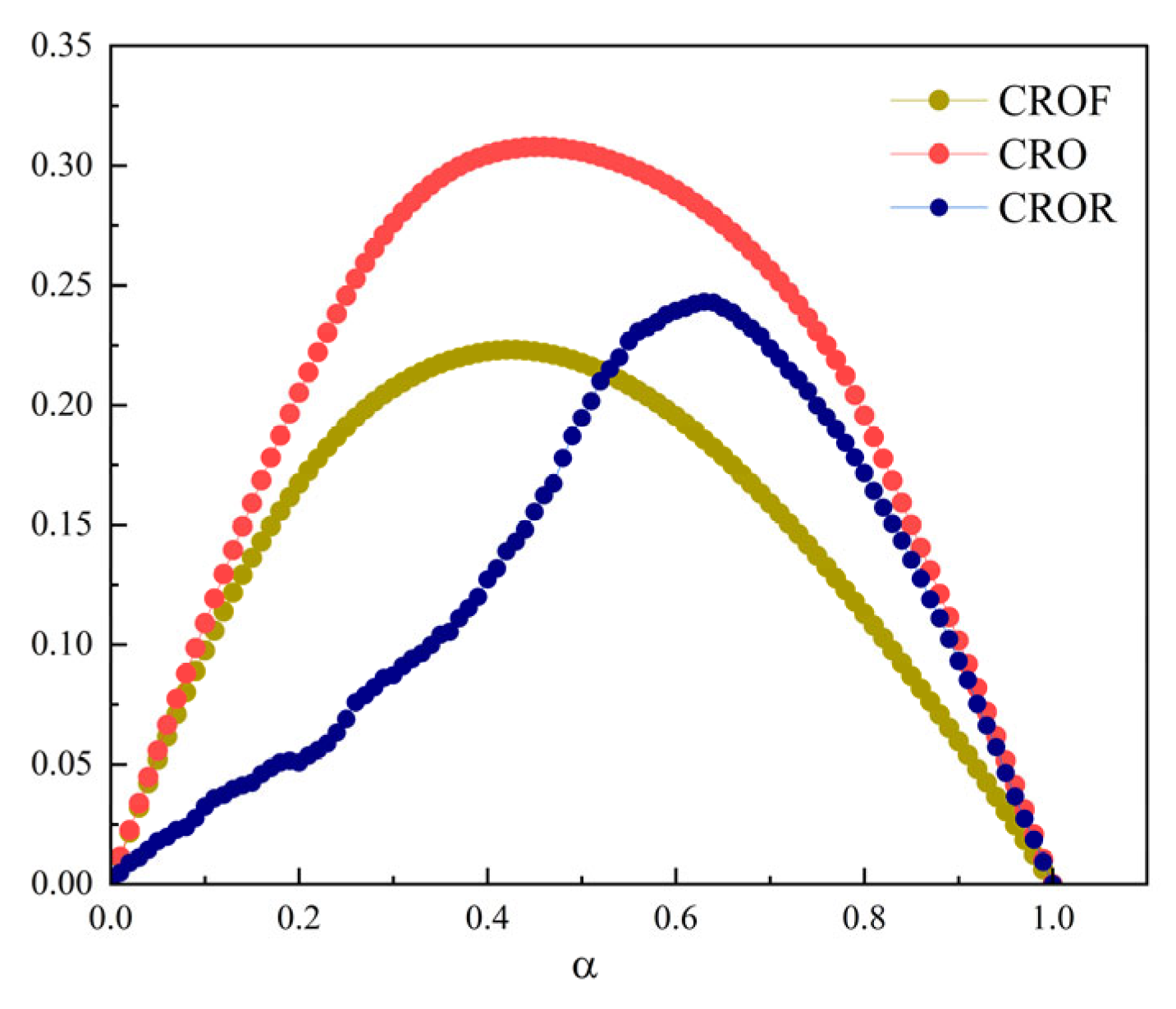
• Two types of complementary indicators are defined, aiming at total output smoothing and source-load matching, respectively. The significance of two types of complementary indicators in different regions is studied. Moreover, the complementary rate of fluctuation (CROF), complementary rate of ramp (CROR), and complementary rate of offset (CRO) are added to the correlation analysis to consider the volatility of VRE output itself. The photovoltaic capacity ratio corresponding to the maximum CROF is proposed as the basis for the hybrid system’s capacity allocation to stabilize the wind and solar output volatility.
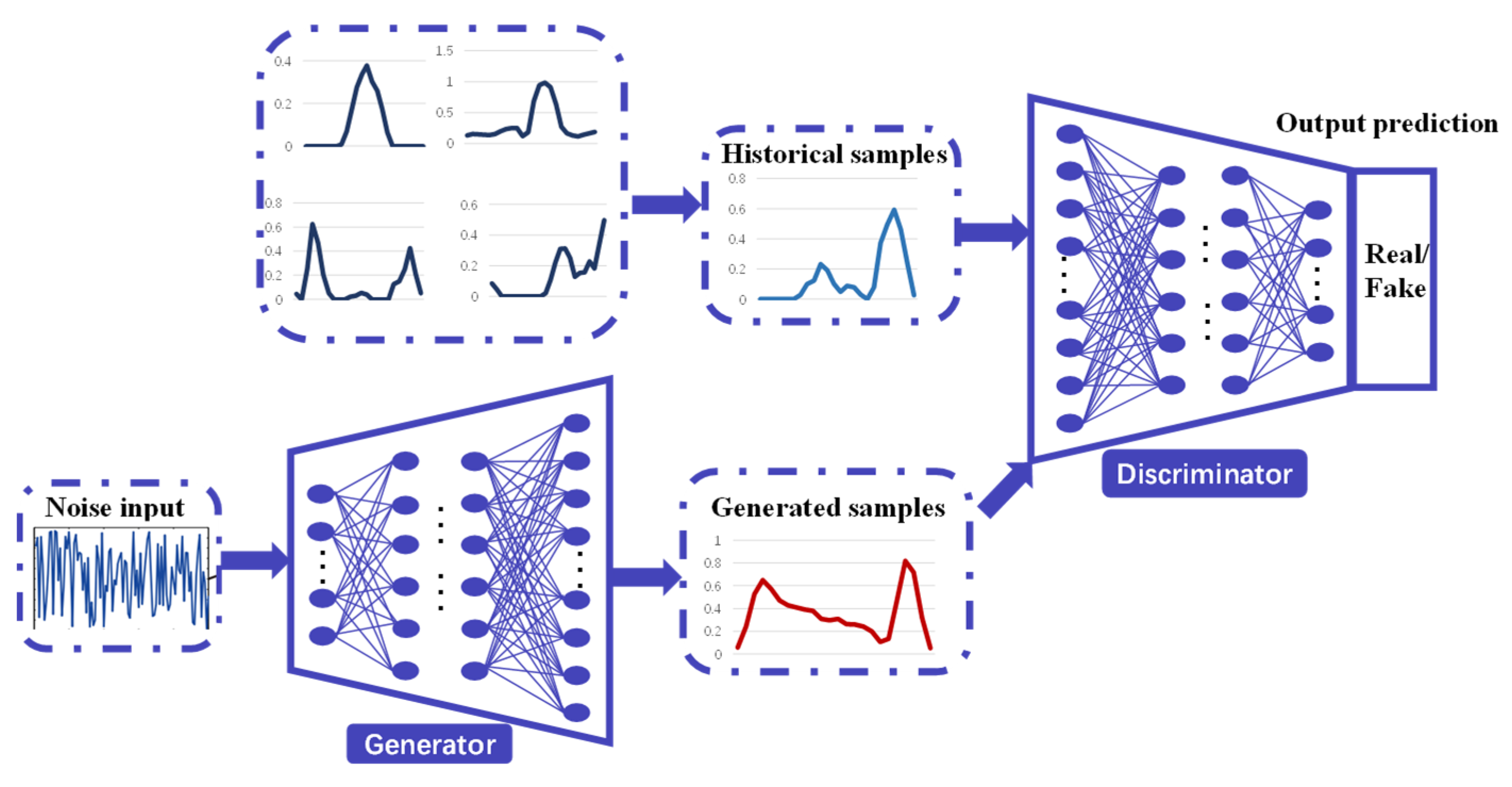
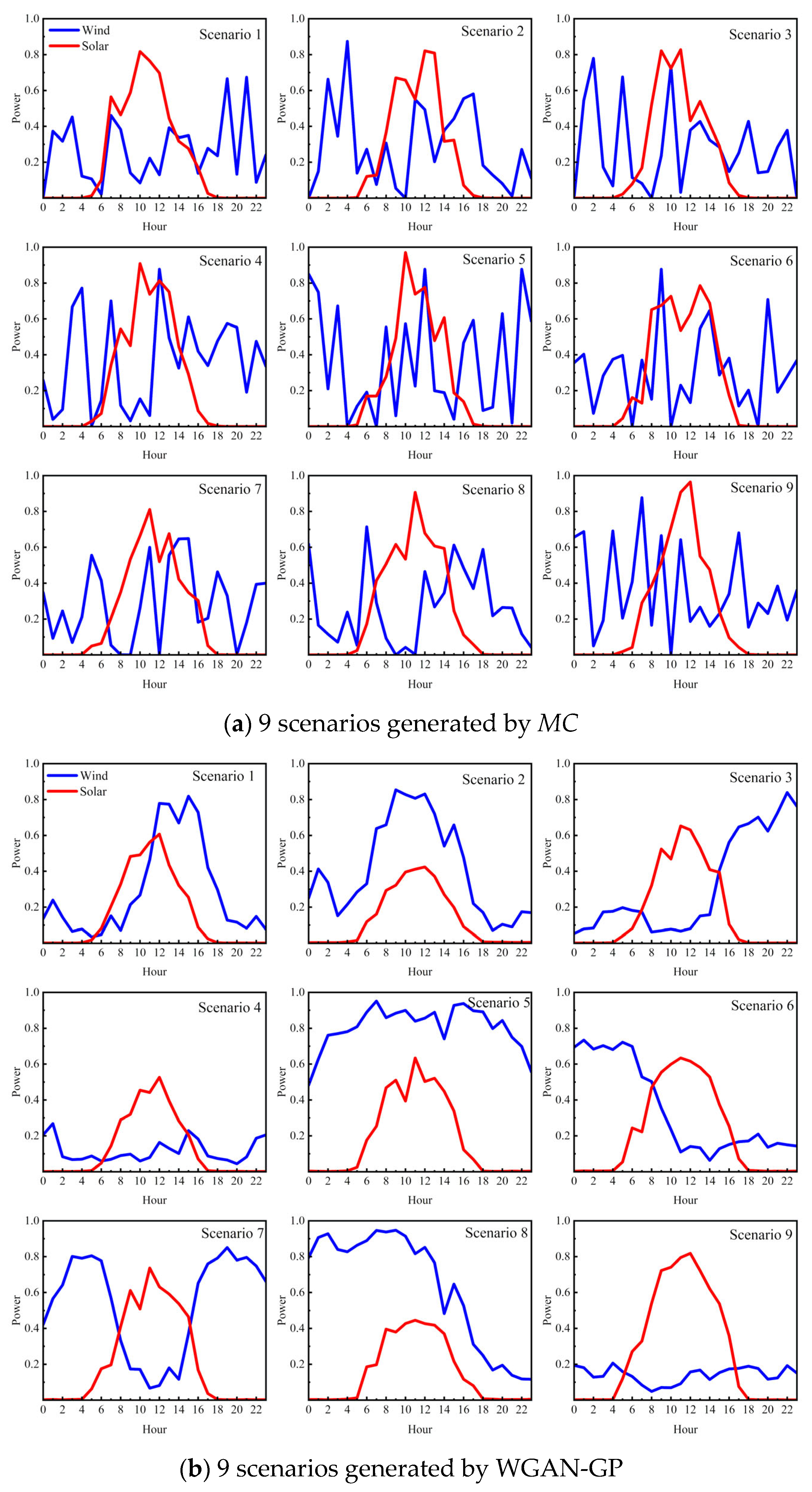
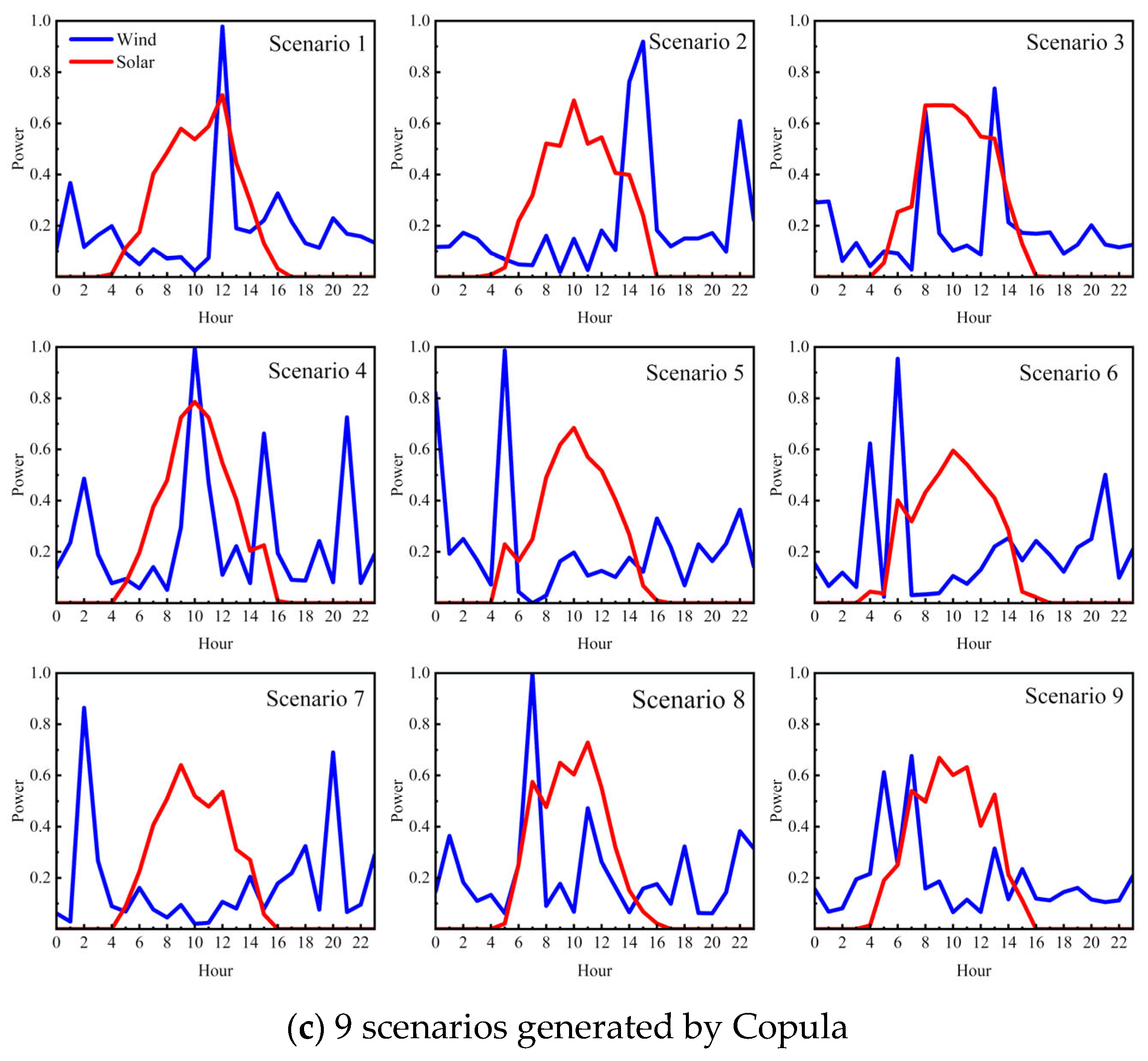
• WGAN-GP, based on a data-driven deep learning method, is used for wind and solar scenario generation, and an unsupervised k-means clustering method is used for scenario reduction. At the same time, we compared the traditional statistical methods of MC and Copula, and the results showed that WGAN-GP generated scenarios could be applied to the VRE output complementary study, which may balance the relevance of the historical with the uncertainty in future production.

The rest of this paper is organized as follows. In Section 2, complementary indicators are illustrated. In Section 3, the study on complementary characteristics of wind and solar energy in wide areas in Haixi, Qinghai, is conducted. Section 4 applies the data-driven and traditional scenario generation methods to the complementary analysis in the chosen regions. Conclusions are drawn in Section 5.

2. Complementary Indicators of Wind and Solar Hybrid System

2.1. Two Types of Complementary Indicators

The complementary characteristics of wind and solar energy in this paper are studied using the energy correlation and the hybrid system’s source-load correlation. We define the correlation coefficient between the output curves of two new energy stations as the first type of complementary indicator, notated as $\tau$. The more negative and smaller the τ indicator is, the more evident it is that the two trends have opposite patterns, indicating a stronger level of complementarity of the first type. The total output curve should closely align with the load demand curve to achieve the best complementary wind and solar hybrid systems strategy. Therefore, the inverse of the correlation coefficient between the total output curve of the hybrid system and the load demand curve is defined as the second type of complementary indicator, denoted as ${\tau }_L$. Smaller and more negative values of ${\tau }_L$ suggest a stronger association between the output curve and load demand curve, indicating a higher level of complementarity of the second type.

2.2. Correlation Coefficient

2.2.1. Pearson Correlation Coefficient

The Pearson correlation coefficient applies to continuous variables, requiring them to conform to a normal distribution, calculated as follows:

$$r_p=\frac{{\sum }_{i=1}^n\left(x_i-\overline{x}\right)\left(y_i-\overline{y}\right)}{\sqrt{{\sum }_{i=1}^n{\left(x_i-\overline{x}\right)}^2}\sqrt{{\sum }_{i=1}^n{\left(y_i-\overline{y}\right)}^2}}$$

(1)

where n is the sample size, $x_i$, and $y_i$ are the individual sample points indexed with $i$, $\overline{x}$ is the sample mean, and analogously for $\overline{y}$.

2.2.2. Spearman Correlation Coefficient

The Spearman correlation coefficient measures the strength and direction of the association between two ranked variables, computed as follows:

$$r_s=1-\frac{6\sum d_i^2}{n\left(n^2-1\right)}$$

(2)

where $d_i=R\left(x_i\right)-R\left(y_i\right)$ is the difference between the two ranks of each observation.

2.2.3. Kendall Correlation Coefficient

The Kendall correlation coefficient is a statistic used to measure the ordinal association between two measured quantities:

$${\tau }_k=\frac{C_{\tau }-D_{\tau }}{{\displaystyle \frac{1}{2}}n\left(n-1\right)}$$

(3)

where $C_{\tau }$ is the number of concordant pairs, and $D_{\tau }$ is the number of discordant pairs.

The above three correlation coefficients all fall within the range [−1, 1], and the closer the result is to 1, the stronger the positive correlation between the two variables. The closer the result is to −1, the stronger the complementarity between the two variables.

2.2.4. Complementary Rate of Fluctuation (CROF)

To quantitatively describe the fluctuations in the adjacent moments of wind speed time series over a while, the corresponding change in wind speed at the adjoining point is defined as one fluctuation. The complementary rate of fluctuation is quantified based on the fluctuation rate of the hybrid system:

$$CROF=1-\frac{{\sum }_{i=1}^n\left|{\alpha }_1{\gamma }_i^1+{\alpha }_2{\gamma }_i^2+\cdots +{\alpha }_k{\gamma }_i^k\right|}{{\alpha }_1{\sum }_{i=1}^n\left|{\gamma }_i^1\right|+{\alpha }_2{\sum }_{i=1}^n\left|{\gamma }_i^2\right|+\cdots +{\alpha }_k{\sum }_{i=1}^n\left|{\gamma }_i^k\right|}$$

(4)

where ${\gamma }_i^k$ represents the volatility rate of the kth VRE power system at point $i$, and ${\alpha }_k$ is the kth VRE capacity ratio in the hybrid system. The value range of CROF is $\left[0, 1\right]$. The greater the value, the better the hybrid system’s complementary.

2.2.5. Complementary Rate of Ramp (CROR)

To quantitatively describe the fluctuation in the non-adjacent moments of the wind speed time series over a while, the process of wind speed extremum in the time series to the next extremum and the two extreme points at the non-adjacent time is defined as a single ramp. The ramp process refers to the continuous ascent or continuous descent characteristic of the output power curve of the hybrid system over a continuous time window, calculated as follows:

$$CROR=1-\frac{RROC}{{\alpha }_{1}R{R}^1+{\alpha }_{2}R{R}^2+\cdots +{\alpha }_{k}R{R}^k}$$

(5)

where RROC is the ramp rate of the hybrid system, and $R{R}^k$ is the ramp rate of the kth VRE power system. The value range of CROR is $\left[0, 1\right]$. The greater the value, the more pronounced the ramp complementarity of the hybrid system is.

2.2.6. Complementary Rate of Offset (CRO)

Offset refers to the deviation between the actual output power of VRE and the average output from moment to moment, similar to other complementary rate calculations, also calculated by offset rate between the hybrid system and single VRE power system:

$$CRO=1-\frac{{\displaystyle \frac{1}{n}}{\sum }_{i=1}^n{\displaystyle \frac{\left|P_j^i-{\overline{P}}_j\right|}{{\overline{P}}_j}}}{{\alpha }_1{\epsilon }^1+{\alpha }_2{\epsilon }^2+\cdots +{\alpha }_k{\epsilon }^k}$$

(6)

where $P_j^i$ is the output power of the hybrid system at point $i$, ${\overline{P}}_j$ is the average of the hybrid system, and ${\epsilon }^k$ is the offset rate of the kth VRE power system.

3. Study on Complementary Characteristics of Wind and Solar

3.1. Data

We have collected reanalysis data for five years, from 2015 to 2020, in eight regions of Haixi, including wind speed, wind direction, temperature, and solar irradiation. The data were recorded hourly. For Part 3 of the study, we utilized the 2020 data, while the 2015–2019 data were used in Part 4 for scenario generation research. As shown in

Table 2. The basic information about the selected regions.

Region	Location	Longitude	Latitude	Mean Solar Irradiance (W/m2)	Mean Wind Speed (m/s)
1	Wulan	99.20 E	36.34 N	203.64	5.04
2	Dachaidan	95.11 E	37.35 N	223.65	6.02
3	Delingha	97.24 E	37.06 N	202.91	6.56
4	Dulan	96.25 E	36.22 N	219.64	6.24
5	Golmud	95.5 E	36.23 N	220.47	5.86
6	Mangnai	92.48 E	37.95 N	221.83	5.71
7	Lenghu	93.27 E	35.54 N	208.59	5.30
8	Tianjun	98.49 E	37.22 N	199.13	5.35

, the average annual wind speed in the eight regions is above 5 m/s, and the mean solar irradiation intensity is above 200 W/m², except for region 8. The average monthly and yearly peak sunshine hours (PSH) in Haixi are presented in

Table 3. Peak sunshine hours in Haixi.

Month	1	2	3	4	5	6	7	8	9	10	11	12	Mean
PSH (h)	3.20	4.13	5.17	6.11	6.29	6.06	5.99	5.71	5.01	4.49	3.50	2.89	4.88

, and the annual mean PSH is 4.88 h, the highest in Qinghai Province. Moreover, the Gobi Desert area, which is situated in Haixi, contains the most wind and solar energy-rich regions that require low operation and maintenance costs, thereby highlighting the benefits of wind and solar energy potential in Haixi.

3.2. Data-Processing

3.2.1. Output Power of Photovoltaic (PV) Power Station

The optimal slope angle of the PV power station is 38° in Haixi, and the azimuth angle of the array is taken to be south, i.e., 0°. We assume the installed capacity is 100 MW in each PV power station. Thus, the PV power station output power calculation model is as follows:

$$P_{sj}={\sum }_{i=1}^n \frac{G_T^i}{G_{STG}}\times P_{cs}\times R_{PV}$$

(7)

where $P_{sj}$ is the output power of the PV power station at the jth region, $G_T^i$ is the total radiation of the slanted plane at point $i$, W/m², G_STG is the standard irradiance, 1000 W/m², P_cs is the installed capacity of the PV power station, and R_PV is the comprehensive efficiency of the PV power station, 0.81.

3.2.2. Output Power of Wind Farm

In this case, we have utilized the power curve of a 3.0 MW wind turbine to convert wind speed data into wind power data. The chosen wind turbine has a cut-in wind speed, rated wind speed, and cut-out wind speed of 3 m/s, 11.5 m/s, and 25 m/s, respectively, with a hub height of 100 m. Assuming an installed capacity of 100 MW in each wind farm, the wind farm output power calculation model is as follows:

$$P_{wj}={\sum }_{i=1}^n \frac{P_T^i}{P_{WG}}\times P_{cw}\times R_V$$

(8)

where $P_{wj}$ is the output power of the wind farm at the jth region, $P_T^i$ is the actual output power of a single wind turbine at point $i$, P_WG is the rated capacity of the wind turbine, P_cw is the installed capacity of the wind farm, and R_V is the comprehensive efficiency of the wind farm, 0.7.

3.2.3. Normalization

Normalizing the wind and solar output data is necessary to eliminate the dimensional influence, and this paper uses the max-min value method for normalization.

$$P_{ns}^i=\frac{P_S^i-P_S^{min}}{P_S^{max}-P_S^{min}}$$

(9)

$$P_{nw}^i=\frac{P_W^i-P_W^{min}}{P_W^{max}-P_W^{min}}$$

(10)

where $P_S^i$, $P_W^i$ is the output power of the PV power station and wind farm at a specific moment. $P_S^{max}$, $P_S^{min}$ is the maximum and minimum of the output power of the PV power station at the time series, respectively. $P_W^{max}$, $P_W^{min}$ is the maximum and minimum of the output power of the wind farm at the time series, respectively. $P_{ns}^i$, $P_{nw}^i$ is the normalized values of the PV power station and the wind farm output power, respectively. The output data would be in the range of [0, 1] after normalization.

3.2.4. Output Power of the Hybrid System

Assume the photovoltaic capacity ratio in the wind and solar hybrid system is $\alpha$, and the wind energy capacity ratio is $\left(1-\alpha \right)$. The total theoretical output power of the hybrid system is calculated as follows:

$$P_j={\sum }_{i=1}^n\left[\alpha P_{ns}^i+\left(1-\alpha \right)P_{nw}^i\right]$$

(11)

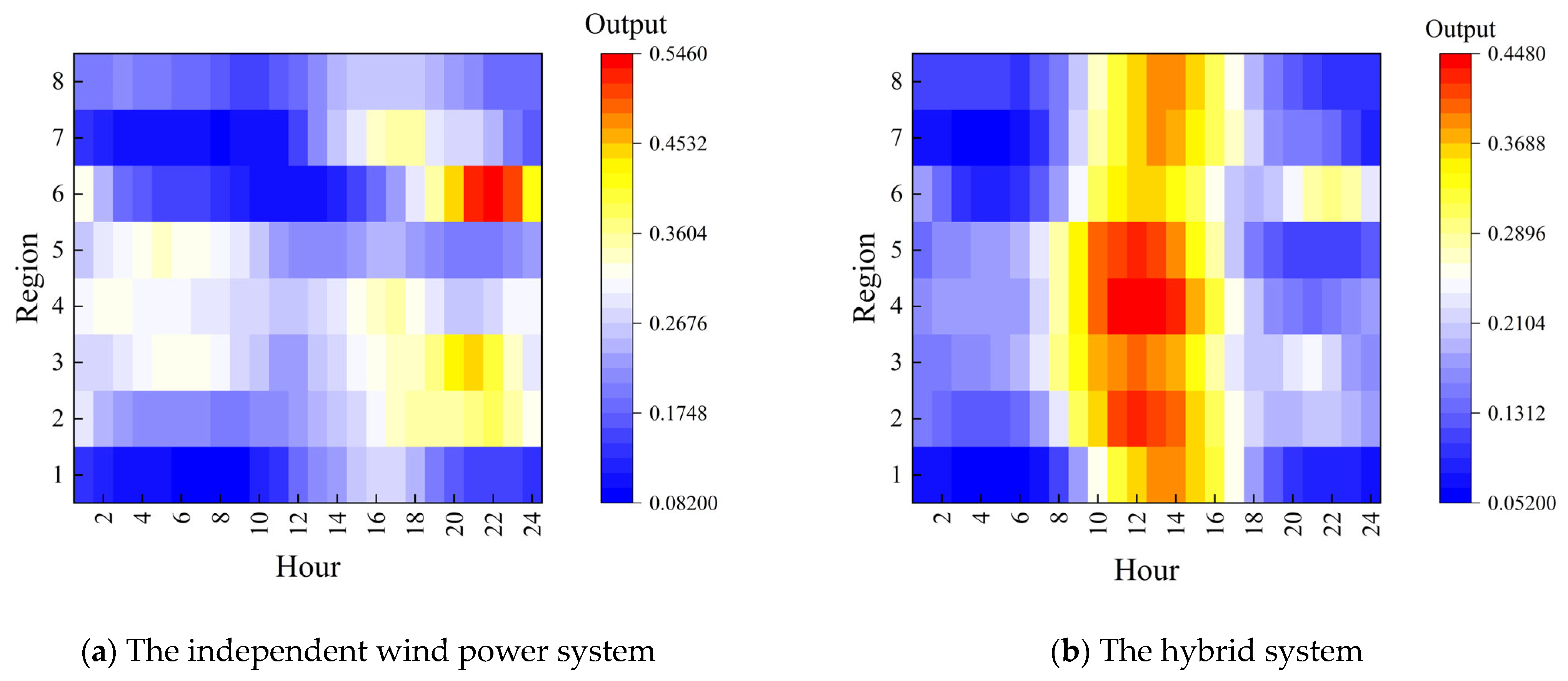
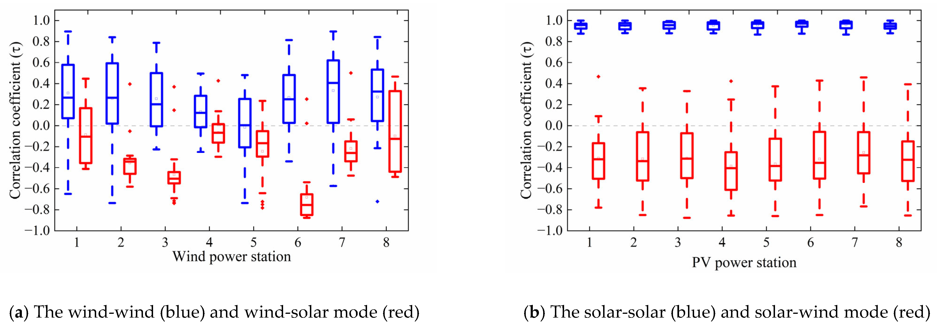
3.3. The First Type of Complementarity

The first type of complementarity defined in this paper pertains to the complementarity between wind and solar resources. Figure 1 displays the annual photovoltaic and wind power output in Region 3. However, the regularity of the wind and solar output complementarity is not evident. Additionally, the volatility and intermittency of the two resources are observed, as well as in other regions. Hence, analyzing the synergistic effects of wind and solar resource output at various temporal and spatial scales is necessary.

Firstly, the complementarity of wind and solar energy resources at the exact spatial location is analyzed. The Kendall, Spearman, and Pearson correlation coefficients of wind and solar resources in eight regions of Haixi are calculated in

Table 4. The correlation coefficient in the selected regions.

Region	Kendall	Spearman	Pearson
1	0.0392	0.1051	0.0281
2	−0.0966	−0.0643	−0.0706
3	−0.1042	−0.1139	−0.0754
4	−0.0255	−0.0348	−0.0184
5	−0.0089	−0.0488	−0.0068
6	−0.2956	−0.2772	−0.2184
7	−0.1214	−0.0727	−0.0878
8	0.0625	−0.0050	0.0452

.

Figure 2 depicts the degree of wind and solar energy complementarity with the deeper green, indicating higher complementarity levels. Conversely, deeper red represents stronger positive correlations between the two VREs. The complementarity of wind and solar in Mangnai is significant. Furthermore, positive correlations exist between wind and solar in Tianjun and Wulan. However, the complementarity between different VREs is not limited to the exact spatial location, especially considering the development of large-scale wind and solar bases across China. Hence, this paper also examines wind and solar complementarity at different spatial sites, including four scenarios: wind-wind, wind-solar, solar-solar, and solar-wind.

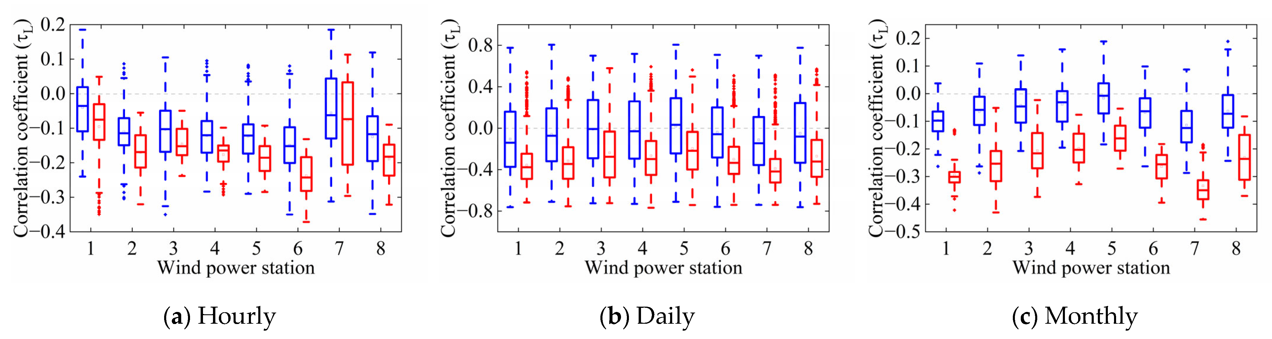
3.3.1. Wind-Wind and Wind-Solar Mode

Eight selected regions were studied to evaluate the complementarity between wind power in a specific location and wind (solar) power in different spatial areas. Figure 3 shows box charts of the first type of complementary indicator on the hourly, daily, and monthly scales.

We can conclude that the wind-solar mode could enhance complementarity across different time scales, particularly when total output smoothing is prioritized. In addition, the first type of complementarity in the selected area is most significant on the daily scale. Therefore, the complementarity of wind and solar can eliminate inverse peak regulation characteristics and improve the accommodation of new energy resources.

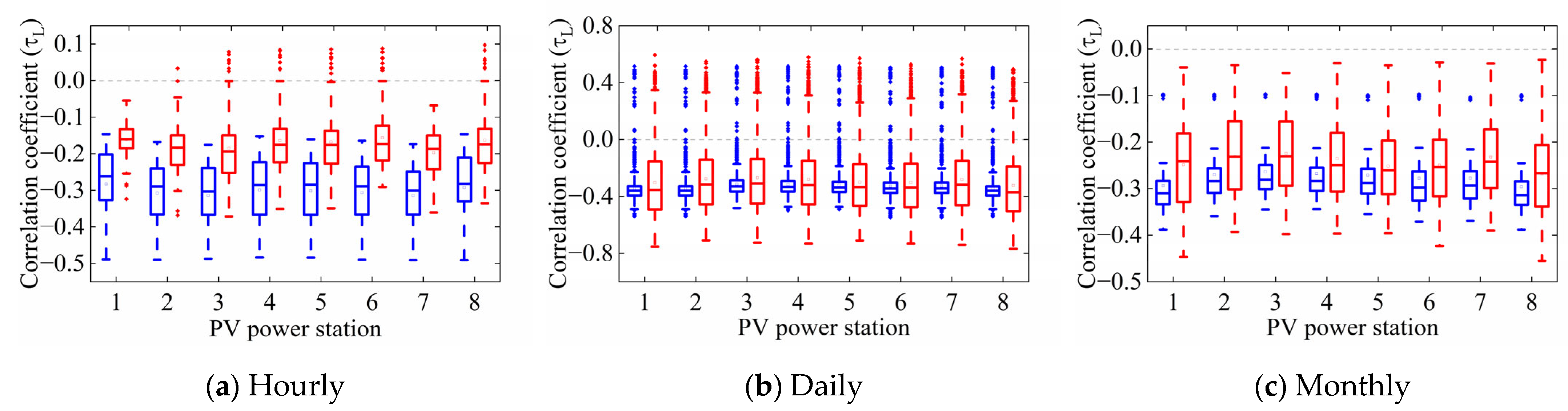
3.3.2. Solar-Solar and Solar-Wind Mode

Figure 4 shows box charts of the first type of complementary indicator on the hourly, daily, and monthly scales.

Figure 4 illustrates that the solar resources in Haixi are highly correlated. This is due to Haixi’s location in the Qaidam Basin, which is primarily composed of desert and wasteland, resulting in no discernible differences in radiation intensity and PSH. When striving for total output smoothing, the solar-wind complementary mode has a more significant effect than the solar-solar complementary mode. Specifically, the first type of complementarity in the solar-wind mode is more pronounced. Regarding the timescale of the solar-wind mode, the correlation intensity varies from strong to weak in the following order: daily, monthly, and hourly. The stable output of PV power stations at the daily scale can be significantly improved through solar-wind complementation, particularly when there is zero output at night. Climate mainly affects the output power of PV power stations at a monthly scale, which makes it easy to summarize the regularity. Solar-wind complementation can help improve low output levels during winter. Solar energy production fluctuates wildly at the hourly scale, and the regularity is weak. Therefore, the complementary effect of wind and solar is not very significant.

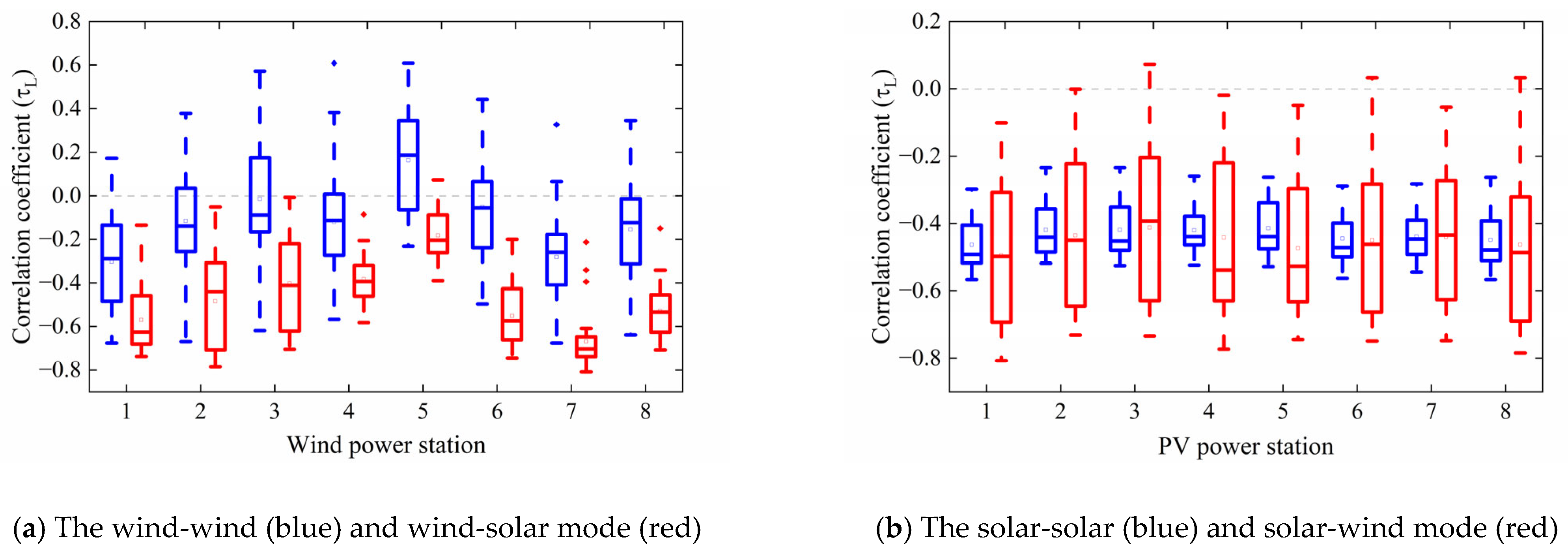
3.4. The Second Type of Complementarity

In the operation of wind and solar hybrid systems, it is often necessary to dynamically adjust the capacity ratio according to load requirements to achieve the optimal complementary operating effect. By Formulas (4)–(6), in addition to the volatility of the resource, the photovoltaic capacity ratio is also a factor affecting complementary results. Figure 5 shows the trend of CROF, CRO, and CROR with photovoltaic capacity ratio $\alpha$.

Figure 5 shows that the three complementary indicators in the operation stage tend to increase first and decrease later as the photovoltaic capacity ratio gradually increases to one. Still, the $\alpha$ values corresponding to the peak point are different. Among them, the peak point of CROR corresponds to the most considerable $\alpha$ value, indicating that solar energy contributes more to offset complementarity. The peak point of CROF corresponds to the smallest $\alpha$ value, meaning that wind energy is more sensitive to volatility. In this paper, the individual output of wind resources in each region and the combined output of wind and solar hybrid systems are calculated, respectively. The $\alpha$ value of the hybrid system is determined according to the peak point of CROF in each region. The results are shown in Figure 6.

Figure 6 shows that wind power support capability is weak during the morning peak hours, photovoltaics has almost no output during the evening peak hours, and the output level of new energy is limited. It is tough to ensure a power supply in extreme weather, such as in extreme heat and in no-wind conditions. Wind resource output shows inverse peak regulation characteristics in most regions except a few. However, when combining wind and solar energy in the same area, the total output power of all regions is higher during the day than at night. The maximum output occurs between 11 o’clock and 15 o’clock, which compensates for zero solar production at night, meets the load demand, and is easier to consume.

3.4.1. Wind-Wind and Wind-Solar Mode

Figure 7 displays box charts for the second type of complementary indicator on hourly, daily, and monthly scales. When the goal is to meet the load requirements as much as possible, the second type of complementarity of wind-solar is more significant than wind-wind mode on all three timescales. Moreover, in 8 different regions, this complementarity is most prominent on a daily scale.

3.4.2. Solar-Solar and Solar-Wind Mode

Figure 8 displays box charts for the second type of complementary indicator on hourly, daily, and monthly scales. In terms of matching energy sources with load requirements, the second type of complementarity of solar-wind mode is not as evident as the first type, especially when considering hourly fluctuations.

To summarize, the study on the first type of complementary characteristics showed that both the wind-solar and solar-wind modes could enhance the overall smoothness of energy output. Meanwhile, the study on the second type of complementary characteristics showed that the wind-solar mode proved beneficial for matching sources to load requirements, but the same could not be said for the solar-wind mode. In fact, the solar-solar complementary mode performed better in meeting load requirements, with the most significant improvement being observed on a daily scale.

Furthermore, Section 3.3 and Section 3.4 led us to the following conclusions. Firstly, the best complementary outcome for wind-solar mode was found in region six concerning the first type of complementarity. Conversely, the wind-solar mode’s most significant impact in relation to the second type of complementarity was observed in both region six and region seven. Moreover, statistical data indicated that the most substantial impact in the first type of complementarity occurs when wind energy from region six is combined with solar energy from region seven, forming a hybrid system. On the other hand, the second type of complementarity was most evident when wind energy from region seven was combined with solar energy from region three.

4. Scenario Generation and Complementary Analysis Based on WGAN-GP

4.1. Scenario Generation of Wind and Solar Output Based on WGAN-GP

Accurately constructing VRE output scenarios is significant for promoting VRE’s accommodation and optimal operation in multi-energy power systems. Traditional scenario generation methods based on the probabilistic model do not consider various correlations and unknown relationships of VRE output. At the same time, finding a model widely applicable to actual complexities is difficult. GAN [41] is a generative model based on the adversarial theory, mainly consisting of the generator and discriminator. The input of the discriminator is the real samples and the generated samples, and the task of the discriminator is to separate the real samples from the fake samples. Finally, the model finds the smallest value of the cost function of the generator and discriminator to achieve the Nash equilibrium. The objective function of the GAN to complete adversarial training is as follows, and the entire optimization process can be considered a maximum-minimization problem:

$$\underset{G}{min}\underset{D}{max} V\left(D,G\right)=E_{x\sim p_r}\left[logD\left(x\right)\right]+E_{z\sim p_g}\left[log\left(1-D\left(G\left(z\right)\right)\right)\right]$$

(12)

where $P_r$ is the probability distribution of real data, and $P_g$ is the probability distribution of generated data.

However, there is a problem with the original GAN. If the discriminator is too powerful, the generator may face the problem of gradient disappearance and make the loss function unable to converge. Furthermore, if the generator is too well trained, the discriminator may face the problem of gradient explosion. Therefore, WGAN [42] introduces the Wasserstein distance into the model to ensure gradient smoothness. When the real data has little or no overlap with generated data, the distance between the two can still be measured to provide meaningful gradient information. The Wasserstein distance is defined as follows:

$$W\left(P_r,P_g\right)=\underset{\gamma ~\prod \left(P_r,P_g\right)}{inf}{E}_{\left(x,y\right)~\gamma } \left[\parallel x-y\parallel \right]$$

(13)

where $\prod \left(P_r,P_g\right)$ denotes the set of all joint distributions $\gamma \left(x,y\right)$ whose marginals are $P_r$ and $P_g$, respectively. Intuitively, $\gamma \left(x,y\right)$ indicates how much “mass” must be transported from $x$ to $y$ to transform the distributions $P_r$ into the distribution $P_g$.

Although WGAN training does not require the generator and discriminator to achieve Nash equilibrium, the generator can generate good samples so long as the discriminator is well-trained to avoid gradient explosions. However, weight clipping in WGAN, which limits the parameters in the model to a specific range, will weaken the modeling capability and may cause the gradient explosion again when the clipping range approaches the limit value. To avoid this problem effectively, the WGAN-GP model [43] introduces gradient penalty (GP) terms to improve the influence of weight clipping constraint parameters used in WGAN to satisfy 1-Lipschitz continuity conditions on the network. The gradient penalty is defined as follows:

$$GP=\lambda E_{\widehat{x}~\chi }{\left[\parallel {\nabla }_{\widehat{x}}D\left(\widehat{x}\right){\parallel }_2-1\right]}^2$$

(14)

where $\lambda$ is the gradient penalty coefficient, $\chi$ sampling uniformly along straight lines between pairs of points sampled from the data distribution $P_r$ and the generator distribution $P_r$. The objective function is as follows:

$$L=E_{\tilde{x}~p_g}\left[D\left(\tilde{x}\right)\right]-E_{x~p_r}\left[D\left(x\right)\right]+\lambda E_{\widehat{x}~\chi }{\left[\parallel {\nabla }_{\widehat{x}}D\left(\widehat{x}\right){\parallel }_2-1\right]}^2$$

(15)

This paper selected five years of data (from 1 January 2015 to 31 December 2019) from eight Haixi, Qinghai Province regions as the database. The temporal resolution is 1 h, and 24 sets of wind and solar output data were used as a single sample, with a total of 14,608 samples. The basic structure is shown in Figure 9. Algorithm 1 shows the Pseudocode of WGAN-GP. The WGAN-GP model was built using the Pytorch deep learning framework and accelerated via a CUDA parallel computing on a GPU in the simulation. The computer employed an Intel Xeon E5-2678 v3 2.50 GHz CPU with 128 GB memory, and a NVIDIA GeForce RTX 2080 Ti GPU with 11 GB of graphics memory (The server is rented on the website: https://matgo.cn/). The case study first validated the effectiveness of the proposed method for generating scenarios, and then performed a simulation comparison between the WGAN-GP method and the traditional scenario generation methods.

Figure 9. The architecture of GAN used for wind/solar scenario generation.

Figure 9. The architecture of GAN used for wind/solar scenario generation.

Algorithm 1: Pseudo-code of WGAN-GP

Algorithm WGAN-GP. We use default values of $\lambda =10$, $n_{critic}=5$, $\alpha =0.0002$, ${\beta }_1=0.5$, ${\beta }_2=0.999$

Require: The gradient penalty coefficient $\lambda$, the number of critic iterations per generator iteration $n_{critic}$, the batch size $m$, Adam hyperparameters $\alpha$, ${\beta }_1$, ${\beta }_2$.

Require: initial critic parameters ${\omega }_0$, initial generator parameters ${\theta }_0$

1: While $\theta$ has not converged do

2:    for $t=1,\dots , n_{critic}$do

3:      for $i=1,\dots , m$ do

4:         Samples real data $x~P_r$, latent variable $z~p\left(z\right)$, a random number $ϵ~U\left[0, 1\right]$

5:         $\tilde{x}\leftarrow G_{\theta }\left(z\right)$

6:         $\widehat{x}\leftarrow ϵx+\left(1-ϵ\right)\tilde{x}$

7:         $L^{\left(i\right)}\leftarrow D_{\omega }\left(\tilde{x}\right)-D_{\omega }\left(x\right)+\lambda {\left(\parallel {\nabla }_{\widehat{x}}{D}_{\omega }\left(\widehat{x}\right){\parallel }_2-1\right)}^2$

8:      end for

9:      $\omega \leftarrow Adam\left({\nabla }_{\omega }\frac{1}{m}{\sum }_{i=1}^m{L}^{\left(i\right)},\omega , \alpha , {\beta }_1, {\beta }_2\right)$

10:    end for

11:    Sample a batch of latent variables ${\left\{z^{\left(i\right)}\right\}}_{i=1}^m~p\left(z\right)$

12:    $\theta \leftarrow Adam\left({\nabla }_{\theta }\frac{1}{m}{\sum }_{i=1}^m-D_{\omega }\left(G_{\theta }\right)), \theta , \alpha , {\beta }_1, {\beta }_2\right)$

13: end while

4.2. Scenario Generation Results by Three Methods

Part 3 provides a detailed analysis of wind and solar energy complementarity in the Haixi region. The study found the optimum combination of the first and second types of complementarity. However, the results are based on data from a single year and are significantly impacted by the unpredictability of wind and solar energy output. In order to enhance the research on wind and solar complementarity, this study utilizes a scenario analysis method. Firstly, a large number of wind and solar output scenarios are generated using WGAN-GP, with scenario reduction completed using k-means clustering.

Furthermore, the study also analyzes scenario generation methods based on statistics, including the Monte Carlo (MC) and Copula function (Copula), to compare results obtained using WGAN-GP. Figure 10 shows the scenario generation results for Region 4. However, this paper does not include the results for other regions due to space limitations.

The root mean square error (RMSE) and mean absolute error (MAE) of the generated most probable output data are calculated to test the results of scenario generation, as shown in

Table 5. The error of the generated data.

	WGAN-GP		Copula		MC
	RMSE	MAE	RMSE	MAE	RMSE	MAE
$P_{s1}$	0.036	0.024	0.089	0.059	0.112	0.059
$P_{w1}$	0.091	0.079	0.100	0.083	0.321	0.214
$P_{s2}$	0.056	0.033	0.109	0.065	0.167	0.090
$P_{w2}$	0.158	0.150	0.172	0.154	0.251	0.212
$P_{s3}$	0.041	0.027	0.112	0.068	0.085	0.049
$P_{w3}$	0.172	0.139	0.170	0.155	0.325	0.267
$P_{s4}$	0.047	0.026	0.092	0.053	0.084	0.047
$P_{w4}$	0.190	0.182	0.204	0.181	0.207	0.163
$P_{s5}$	0.086	0.054	0.113	0.069	0.126	0.061
$P_{w5}$	0.134	0.122	0.172	0.134	0.245	0.208
$P_{s6}$	0.065	0.044	0.073	0.048	0.140	0.068
$P_{w6}$	0.088	0.079	0.191	0.151	0.153	0.116
$P_{s7}$	0.024	0.015	0.075	0.049	0.113	0.059
$P_{w7}$	0.095	0.068	0.159	0.100	0.213	0.149
$P_{s8}$	0.039	0.023	0.082	0.051	0.092	0.053
$P_{w8}$	0.091	0.078	0.137	0.128	0.263	0.207
mean	0.088	0.071	0.128	0.097	0.181	0.126
$\Delta$			0.040	0.026	0.093	0.055

.

Table 6. The error of the hybrid system with generated data.

		WGAN-GP		Copula		MC
	$\mathit{\alpha }$	RMSE	MAE	RMSE	MAE	RMSE	MAE
$P_1$	0.35	0.065	0.056	0.085	0.065	0.205	0.132
$P_2$	0.46	0.097	0.090	0.124	0.101	0.165	0.139
$P_3$	0.56	0.085	0.072	0.113	0.095	0.153	0.126
$P_4$	0.42	0.117	0.110	0.134	0.113	0.124	0.099
$P_5$	0.43	0.107	0.091	0.127	0.092	0.147	0.129
$P_6$	0.44	0.039	0.031	0.112	0.090	0.096	0.071
$P_7$	0.45	0.058	0.043	0.097	0.064	0.120	0.085
$P_8$	0.47	0.046	0.038	0.095	0.082	0.139	0.108
mean	0.45	0.077	0.066	0.111	0.088	0.144	0.111
$\Delta$				0.034	0.022	0.067	0.045

shows the hybrid system’s RMSE and MAE composed of the generated wind and solar data. $P_{sj}$, $P_{wj}$ represents the photovoltaic output and wind power output in each region, respectively. $P_j$ denotes the total output after the combination in each region. $\Delta$ represents the error difference between the proposed method and Copula, MC.

The results in Table 5 and Table 6 show that the generated scenarios by WGAN-GP are closer to the actual results than those generated by the traditional statistics-based methods. Furthermore, the effect of Copula is superior compared to the MC method. Additionally, compared with the Copula function method, the RMSE of generated output using the proposed methodology decreased by 4% and 3.4% in independent renewable energy systems and hybrid power systems, respectively. Compared with the MC method, the value comes to 9.7% and 6.7%.

4.3. Complementary Analysis Based on Scenario Generation

In this paper, the generated scenarios with the highest probability generated by WGAN-GP are close to the measured data. At the same time, the data with a lower chance can also characterize the uncertainty and unknowability of the future output. Figure 11 and Figure 12 are box charts of the first and second types of complementarity indicators for WGAN-GP generated data under different complementary modes, respectively.

The WGAN-GP-generated data has led to the following conclusions: Firstly, combining wind and solar energies can significantly improve the first and second types of complementarity. Secondly, the solar-wind complementary mode has been found to improve the first type of complementarity. Although there is a slight deviation from the measured results, it can also somewhat improve the second type of complementarity. However, the effectiveness of this improvement is limited. Nonetheless, it can bolster the measured data’s complementary findings and enhance the overall robustness of the results. Thirdly, wind resources in region six pair best with other regions’ solar energy for total output smoothing, while wind resources in region seven pair best with other regions’ solar energy for source-load matching. Additionally, a positive correlation exists between wind and solar resources in region one and eight, as shown in Figure 3. The generated data can partially restore this feature.

5. Conclusions

This paper explores the complementarity of wide-area wind and solar resources in Haixi from two perspectives: total output smoothing and source-load matching. It defines the first and second types of complementary indicators and analyzes four complementary modes: wind-wind, wind-solar, solar-solar, and solar-wind. Moreover, the study proposes a deep learning-based scenario generation method to comprehensively analyze wind and solar resource complementarity, improving the results’ robustness. The main conclusions are as follows:

• This paper focuses on wind and solar complementarity in Haixi, Qinghai. It proposes using the deep learning method WGAN-GP for complementary studies, which shows that the proposed method can comprehensively analyze the correlation of resource contributions and improve the robustness of the results. This proposed method has a high coverage rate for measured values, which can accurately describe the uncertainty of renewable energy output. In addition, the proposed methodology reduces the RMSE of the generated output by 4% and 3.4% in independent renewable energy systems and hybrid power systems, respectively, compared to the Copula function method. Additionally, compared to the MC method, the RMSE decreases to 9.7% and 6.7%.
• In the first type of complementarity study, wind-solar and solar-wind modes significantly enhance the overall output’s smoothness and stabilize fluctuations in hybrid systems. In the second type of complementarity study, the wind-solar mode also significantly improves source-load matching, making it easier to integrate wind and solar resources to accommodate. However, the solar-wind mode’s improvement effect is less pronounced than that of the first complementarity type.
• In this paper, we found that combining wind energy from region six with solar power from region three showed the best complementary effects in the first type of study. Similarly, combining wind energy from region seven with solar energy from region three yielded the best results in the second type of complementarity study.

References

1. Han, S.; Zhang, L.; Liu, Y.; Zhang, H.; Yan, J.; Li, L.; Lei, X.; Wang, X. Quantitative Evaluation Method for the Complementarity of Wind–Solar–Hydro Power and Optimization of Wind–Solar Ratio. Appl. Energy 2019, 236, 973–984. [Google Scholar] [CrossRef]
2. Weschenfelder, F.; de Novaes Pires Leite, G.; Araújo da Costa, A.C.; de Castro Vilela, O.; Ribeiro, C.M.; Villa Ochoa, A.A.; Araújo, A.M. A Review on the Complementarity between Grid-Connected Solar and Wind Power Systems. J. Clean. Prod. 2020, 257, 120617. [Google Scholar] [CrossRef]
3. Temiz, M.; Dincer, I. Development and Assessment of an Onshore Wind and Concentrated Solar Based Power, Heat, Cooling and Hydrogen Energy System for Remote Communities. J. Clean. Prod. 2022, 374, 134067. [Google Scholar] [CrossRef]
4. Oh, M.; Kim, B.; Yun, C.; Kim, C.K.; Kim, J.-Y.; Hwang, S.-J.; Kang, Y.-H.; Kim, H.-G. Spatiotemporal Analysis of Hydrogen Requirement to Minimize Seasonal Variability in Future Solar and Wind Energy in South Korea. Energies 2022, 15, 9097. [Google Scholar] [CrossRef]
5. El-kenawy, E.-S.M.; Ibrahim, A.; Bailek, N.; Bouchouicha, K.; Hassan, M.A.; Jamei, M.; Al-Ansari, N. Sunshine Duration Measurements and Predictions in Saharan Algeria Region: An Improved Ensemble Learning Approach. Theor. Appl. Climatol. 2022, 147, 1015–1031. [Google Scholar] [CrossRef]
6. François, B.; Borga, M.; Creutin, J.D.; Hingray, B.; Raynaud, D.; Sauterleute, J.F. Complementarity between Solar and Hydro Power: Sensitivity Study to Climate Characteristics in Northern-Italy. Renew. Energy 2016, 86, 543–553. [Google Scholar] [CrossRef]
7. Bird, L.; Lew, D.; Milligan, M.; Carlini, E.M.; Estanqueiro, A.; Flynn, D.; Gomez-Lazaro, E.; Holttinen, H.; Menemenlis, N.; Orths, A.; et al. Wind and Solar Energy Curtailment: A Review of International Experience. Renew. Sust. Energy Rev. 2016, 65, 577–586. [Google Scholar] [CrossRef] [Green Version]
8. Widén, J.; Carpman, N.; Castellucci, V.; Lingfors, D.; Olauson, J.; Remouit, F.; Bergkvist, M.; Grabbe, M.; Waters, R. Variability Assessment and Forecasting of Renewables: A Review for Solar, Wind, Wave and Tidal Resources. Renew. Sust. Energy Rev. 2015, 44, 356–375. [Google Scholar] [CrossRef]
9. dos Anjos, P.S.; da Silva, A.S.A.; Stošić, B.; Stošić, T. Long-Term Correlations and Cross-Correlations in Wind Speed and Solar Radiation Temporal Series from Fernando de Noronha Island, Brazil. Physica A 2015, 424, 90–96. [Google Scholar] [CrossRef] [Green Version]
10. Jani, H.K.; Kachhwaha, S.S.; Nagababu, G.; Das, A. Temporal and Spatial Simultaneity Assessment of Wind-Solar Energy Resources in India by Statistical Analysis and Machine Learning Clustering Approach. Energy 2022, 248, 123586. [Google Scholar] [CrossRef]
11. Xu, L.; Wang, Z.; Liu, Y. The Spatial and Temporal Variation Features of Wind-Sun Complementarity in China. Energy Convers. Manag. 2017, 154, 138–148. [Google Scholar] [CrossRef]
12. Guo, Y.; Ming, B.; Huang, Q.; Yang, Z.; Kong, Y.; Wang, X. Variation-Based Complementarity Assessment between Wind and Solar Resources in China. Energy Convers. Manag. 2023, 278, 116726. [Google Scholar] [CrossRef]
13. Cantão, M.P.; Bessa, M.R.; Bettega, R.; Detzel, D.H.M.; Lima, J.M. Evaluation of Hydro-Wind Complementarity in the Brazilian Territory by Means of Correlation Maps. Renew. Energy 2017, 101, 1215–1225. [Google Scholar] [CrossRef]
14. Kapica, J.; Canales, F.A.; Jurasz, J. Global Atlas of Solar and Wind Resources Temporal Complementarity. Energy Convers. Manag. 2021, 246, 114692. [Google Scholar] [CrossRef]
15. Couto, A.; Estanqueiro, A. Assessment of Wind and Solar PV Local Complementarity for the Hybridization of the Wind Power Plants Installed in Portugal. J. Clean. Prod. 2021, 319, 128728. [Google Scholar] [CrossRef]
16. Frank, C.; Fiedler, S.; Crewell, S. Balancing Potential of Natural Variability and Extremes in Photovoltaic and Wind Energy Production for European Countries. Renew. Energy 2021, 163, 674–684. [Google Scholar] [CrossRef]
17. Lv, A.; Li, T.; Zhang, W.; Liu, Y. Spatiotemporal Distribution and Complementarity of Wind and Solar Energy in China. Energies 2022, 15, 7365. [Google Scholar] [CrossRef]
18. Schindler, D.; Behr, H.D.; Jung, C. On the Spatiotemporal Variability and Potential of Complementarity of Wind and Solar Resources. Energy Convers. Manag. 2020, 218, 113016. [Google Scholar] [CrossRef]
19. Hoicka, C.E.; Rowlands, I.H. Solar and Wind Resource Complementarity: Advancing Options for Renewable Electricity Integration in Ontario, Canada. Renew. Energy 2011, 36, 97–107. [Google Scholar] [CrossRef]
20. Jurasz, J.; Beluco, A.; Canales, F.A. The Impact of Complementarity on Power Supply Reliability of Small Scale Hybrid Energy Systems. Energy 2018, 161, 737–743. [Google Scholar] [CrossRef]
21. Sterl, S.; Liersch, S.; Koch, H.; van Lipzig, N.P.M.; Thiery, W. A New Approach for Assessing Synergies of Solar and Wind Power: Implications for West Africa. Environ. Res. Lett. 2018, 13, 094009. [Google Scholar] [CrossRef]
22. Prasad, A.A.; Taylor, R.A.; Kay, M. Assessment of Solar and Wind Resource Synergy in Australia. Appl. Energy 2017, 190, 354–367. [Google Scholar] [CrossRef]
23. Bett, P.E.; Thornton, H.E. The Climatological Relationships between Wind and Solar Energy Supply in Britain. Renew. Energy 2016, 87, 96–110. [Google Scholar] [CrossRef] [Green Version]
24. Shaner, M.R.; Davis, S.J.; Lewis, N.S.; Caldeira, K. Geophysical Constraints on the Reliability of Solar and Wind Power in the United States. Energy Environ. Sci. 2018, 11, 914–925. [Google Scholar] [CrossRef] [Green Version]
25. Costoya, X.; deCastro, M.; Carvalho, D.; Gómez-Gesteira, M. Assessing the Complementarity of Future Hybrid Wind and Solar Photovoltaic Energy Resources for North America. Renew. Sustain. Energy Rev. 2023, 173, 113101. [Google Scholar] [CrossRef]
26. Hu, J.; Li, H. A Transfer Learning-Based Scenario Generation Method for Stochastic Optimal Scheduling of Microgrid with Newly-Built Wind Farm. Renew. Energy 2022, 185, 1139–1151. [Google Scholar] [CrossRef]
27. Wang, Y.; Ma, H.; Wang, D.; Wang, G.; Wu, J.; Bian, J.; Liu, J. A New Method for Wind Speed Forecasting Based on Copula Theory. Environ. Res. 2018, 160, 365–371. [Google Scholar] [CrossRef] [PubMed]
28. Ma, X.-Y.; Sun, Y.-Z.; Fang, H.-L. Scenario Generation of Wind Power Based on Statistical Uncertainty and Variability. IEEE Trans. Power Syst. 2013, 4, 894–904. [Google Scholar] [CrossRef]
29. Li, J.; Zhou, J.; Chen, B. Review of Wind Power Scenario Generation Methods for Optimal Operation of Renewable Energy Systems. Appl. Energy 2020, 280, 115992. [Google Scholar] [CrossRef]
30. Camal, S.; Teng, F.; Michiorri, A.; Kariniotakis, G.; Badesa, L. Scenario Generation of Aggregated Wind, Photovoltaics and Small Hydro Production for Power Systems Applications. Appl. Energy 2019, 242, 1396–1406. [Google Scholar] [CrossRef] [Green Version]
31. Yang, M.; Liu, W.; Yin, X.; Cui, Z.; Zhang, W. A Two-Stage Scenario Generation Method for Wind-Solar Joint Power Output Considering Temporal and Spatial Correlations. In Proceedings of the 2021 6th Asia Conference on Power and Electrical Engineering (ACPEE), Chongqing, China, 8–11 April 2021; pp. 415–423. [Google Scholar]
32. Wang, Z.; Wang, W.; Liu, C.; Wang, Z.; Hou, Y. Probabilistic Forecast for Multiple Wind Farms Based on Regular Vine Copulas. IEEE Trans. Power Syst. 2018, 33, 578–589. [Google Scholar] [CrossRef]
33. Monforti, F.; Huld, T.; Bódis, K.; Vitali, L.; D’Isidoro, M.; Lacal-Arántegui, R. Assessing Complementarity of Wind and Solar Resources for Energy Production in Italy. A Monte Carlo Approach. Renew. Energy 2014, 63, 576–586. [Google Scholar] [CrossRef]
34. Densing, M.; Wan, Y. Low-Dimensional Scenario Generation Method of Solar and Wind Availability for Representative Days in Energy Modeling. Appl. Energy 2022, 306, 118075. [Google Scholar] [CrossRef]
35. Zhang, H.; Cao, Y.; Zhang, Y.; Terzija, V. Quantitative Synergy Assessment of Regional Wind-Solar Energy Resources Based on MERRA Reanalysis Data. Appl. Energy 2018, 216, 172–182. [Google Scholar] [CrossRef]
36. Ren, G.; Wan, J.; Liu, J.; Yu, D. Spatial and Temporal Assessments of Complementarity for Renewable Energy Resources in China. Energy 2019, 177, 262–275. [Google Scholar] [CrossRef]
37. Chen, Y.; Wang, Y.; Kirschen, D.; Zhang, B. Model-Free Renewable Scenario Generation Using Generative Adversarial Networks. IEEE Trans. Power Syst. 2018, 33, 3265–3275. [Google Scholar] [CrossRef] [Green Version]
38. Zhang, Y.; Ai, Q.; Xiao, F.; Hao, R.; Lu, T. Typical Wind Power Scenario Generation for Multiple Wind Farms Using Conditional Improved Wasserstein Generative Adversarial Network. Int. J. Electr. Power Energy Syst. 2020, 114, 105388. [Google Scholar] [CrossRef]
39. Zhu, J.; Ai, Q.; Chen, Y.; Wang, J. Single-Location and Multi-Locations Scenarios Generation for Wind Power Based on WGAN-GP. J. Phys. Conf. Ser. 2023, 2452, 012022. [Google Scholar] [CrossRef]
40. Tang, J.; Liu, J.; Wu, J.; Jin, G.; Kang, H.; Zhang, Z.; Huang, N. RAC-GAN-Based Scenario Generation for Newly Built Wind Farm. Energies 2023, 16, 2447. [Google Scholar] [CrossRef]
41. Goodfellow, I.; Pouget-Abadie, J.; Mirza, M.; Xu, B.; Warde-Farley, D.; Ozair, S.; Courville, A.; Bengio, Y. Generative Adversarial Networks. arXiv 2014, arXiv:1406.2661. [Google Scholar] [CrossRef]
42. Arjovsky, M.; Chintala, S.; Bottou, L. Wasserstein GAN. arXiv 2017, arXiv:1704.00028. [Google Scholar] [CrossRef]
43. Gulrajani, I.; Ahmed, F.; Arjovsky, M.; Dumoulin, V.; Courville, A. Improved Training of Wasserstein GANs. arXiv 2017, arXiv:1701.07875. [Google Scholar] [CrossRef]
Figure 1. Wind and solar output in Region 3.
Energies 16 03114 g001
Figure 2. The Kendall correlation coefficient of wind and solar in Haixi.
Energies 16 03114 g002
Figure 3. The first type of complementary indicator under different time scales (the blue box represents the wind-wind mode, and the red box illustrates the wind-solar mode).
Energies 16 03114 g003
Figure 4. The first type of complementary indicator under different time scales (the blue box represents the solar-solar mode, and the red box illustrates the solar-wind mode).
Energies 16 03114 g004
Figure 5. The relationship between complementary indicators and photovoltaic capacity ratio.
Energies 16 03114 g005
Figure 6. The independent output of the wind farm and the combined output of the hybrid system.
Energies 16 03114 g006
Figure 7. The second type of complementary indicator under different time scales (the blue box represents the wind-wind mode, and the red box illustrates the wind-solar mode).
Energies 16 03114 g007
Figure 8. The second type of complementary indicator under different time scales (the blue box represents the solar-solar mode, and the red box illustrates the solar-wind mode).
Energies 16 03114 g008
Figure 10. Generated scenarios by three methods in Region 4.
Energies 16 03114 g010aEnergies 16 03114 g010b
Figure 11. The first type of complementary indicator of the WGAN-GP-generated data.
Energies 16 03114 g011
Figure 12. The second type of complementary indicator of the WGAN-GP-generated data.
Energies 16 03114 g012