Article

Improving the Efficiency of Hedge Trading Using Higher-Order Standardized Weather Derivatives for Wind Power

1
Faculty of Transdisciplinary Sciences for Innovation, Kanazawa University, Kanazawa 920-1192, Japan
2
Faculty of Business Sciences, University of Tsukuba, Tokyo 112-0012, Japan
*
Authors to whom correspondence should be addressed.
Energies 2023, 16(7), 3112; https://doi.org/10.3390/en16073112
Submission received: 27 February 2023 / Revised: 23 March 2023 / Accepted: 27 March 2023 / Published: 29 March 2023
(This article belongs to the Special Issue Forecasting and Risk Management Techniques for Electricity Markets II)

Abstract

:
Since the future output of wind power generation is uncertain due to weather conditions, there is an increasing need to manage the risks associated with wind power businesses, which have been increasingly implemented in recent years. This study introduces multiple weather derivatives of wind speed and temperature and examines their effectiveness in reducing (hedging) the fluctuation risk of future cash flows attributed to wind power generation. Given the diversification of hedgers and hedging needs, we propose new standardized derivatives with higher-order monomial payoff functions, such as “wind speed cubic derivatives” and “wind speed and temperature cross-derivatives,” to minimize the cash flow variance and develop a market-trading scheme to practically use these derivatives in wind power businesses. In particular, while demonstrating the importance of standardizing weather derivatives regarding market liquidity and efficiency, we propose a strategy to narrow down the required number (or volume) of traded instruments and improve trading efficiency by utilizing the least absolute shrinkage and selection operator (LASSO) regression. Empirical analysis reveals that higher-order, multivariate standardized derivatives can not only enhance the out-of-sample hedge effect but also help reduce trading volume. The results suggest that diversification of hedging instruments increases transaction flexibility and helps wind power generators find more efficient portfolios, which can be generalized to risk management practices in other businesses.

1. Introduction

In the context of achieving carbon neutrality goals, the penetration of wind power, a typical clean energy source, has been steadily increasing worldwide. According to the International Energy Agency [1], the global wind power capacity is increasing at an accelerating rate and this trend is expected to continue. Small wind turbines, which can be installed at residential sites, have especially attracted attention in recent years, and their market is also expected to grow steadily [2]. With these forces in play, the number and types of players in the wind power markets are also expected to increase worldwide. Then, the need to manage the risk of fluctuations in wind power generation revenues becomes increasingly vital for wind power businesses.
With regard to risk management in wind power generation businesses, in addition to avoiding the risk of loss through accurate forecasting, “hedging” approaches play important roles, which involve the various use of financial transactions/contracts to compensate for inevitable loss risks. Risk management through forecasting approaches is often discussed in the context of avoiding imbalance risk due to high-cost imbalance charges imposed on forecast errors; for example, optimizing market transactions as proposed in [3,4]. However, since it is extremely difficult to accurately forecast and compensate for losses, particularly against the long-term ahead horizon, financial hedging transactions may be used to control such cash flow fluctuation risks. Recently, a method combining both approaches has been proposed, such as the use of derivatives based on prediction errors to hedge against losses derived from prediction errors [5]. Thus, for effective risk management in the electricity business, in addition to improving forecast accuracy, risk “hedging” to compensate for financial losses is vitally essential [6], and a variety of hedging products exist in the electricity market [7]; the focus of this study is also on the latter issue: the concept of hedging.
For hedging “price” risk in the wind power business, financial instruments, such as power futures and bilateral contracts, and support measures, including feed-in tariffs (FIT), can be used. However, few financial instruments are available for hedging “volume” risk in practice. For example, even if a wind power generator has a contract to supply a certain amount of electricity at a fixed price, it may incur losses when electricity cannot be generated owing to poor wind conditions. However, few instruments have been devised to hedge these losses, leaving a room or need for research in developing practical and effective trading schemes to manage the volume risks.
As one of the few instruments for treating these volume risks, Wind Power Futures (WPF) have been listed on the European Energy Exchange (EEX; note that this was delisted in 2020) and Nasdaq. WPFs are contracts with a weighted average of area-wide wind power generation in Germany/Austria as the underlying index. As the underlying index is the amount of electricity generated, the WPF may be effective for large-scale wind power generators in the target area. However, more specific and refined products (derivatives or forwards/futures) may be required for individual power producers, including small-scale wind farms or even households (prosumers) with small wind power generators operating in a specific region. For instance, a more effective tool can be a flexible instrument tailored to the specific weather conditions of the generator’s business area using only observed weather values as the underlying index. These weather derivatives can help ensure transparency as a financial instrument since the generator’s individual situation will not affect the underlying index. Here, we propose an approach for using such “weather” derivatives, while emphasizing transparency and flexibility in product design.
Several studies have examined derivatives for wind power, including not only WPF [8,9] but also the European put-type quanto options [10], wind put barrier options [11], and wind call options [12]. Typically, these derivatives have been studied in the context of pricing rather than how effectively they hedge risk. Papers focusing on the hedge effect of wind derivatives, although very limited, include [13], which analyzed the effectiveness of the WPF, and [14], which showed the effectiveness of option-type derivatives on wind speed. In contrast, Yamada [5] proposed a unique derivative for hedging wind power risk and demonstrated its effectiveness based on non-parametric regression using the generalized additive model (GAM) [15]. The implication presented there is the fact that the hedge effect can be enhanced by estimating arbitrary smooth functions as derivative payoffs rather than using linear or conventional option-type functions (see [16] for the original idea and a genealogy of prior works on this). Subsequently, this hedging approach was extended to multivariate models [17] and also to retailers and solar power producers [18,19] and demonstrated that it also has a high hedge effect for them. In these studies, hedgers use non-parametric regression techniques to estimate smooth payoff functions and obtain optimal weather derivatives. However, derivatives estimated by non-parametric regression require bilateral contracts between insurers and hedgers in practice because the optimal payoffs are hedger-specific. Therefore, there remained room to consider the use of market principles from the perspective of improving the trading efficiency. Therefore, while the derivatives proposed in this present study have the same motivation as these series of studies in terms of constructing arbitrary payoff functions, we propose a new unique “market trading scheme” in which weather derivatives of various types and dimensions are introduced in advance and traded by multiple power utilities (hedgers). In other words, instead of trading (contracting) arbitrary payoff functions, by introducing various types (several to a dozen) of “standardized derivatives,” hedgers with different loss functions (dependent on generation output patterns) can combine the necessary instruments and trade them so that every hedger can replicate their own optimal payoff functions. This would also lead to improve trading efficiency through liquid trading by multiple players (details in Section 2).
For specific modeling, this study draws inspiration from previous research on wind power forecasting models. In some previous studies, wind power generation can be generally modeled in the form of a cubic function of wind speed, and temperature is also often taken into account as the next most influential weather variable after wind speed (see Appendix A). Taking this into account, we apply their insights to design weather derivatives based on wind speed and temperature for wind power businesses. In addition to estimating non-parametric payoffs using a two-dimensional tensor product spline function [20] that can capture the complex interaction of wind speed and temperature on wind power generation, and evaluating the hedge effect of previous methods, we introduce new composite and standardized derivatives, such as the “wind speed cubic derivatives” and “wind speed and temperature cross-derivatives,” and demonstrate the effectiveness of derivative portfolios replicated with them.
As noted above, our primary methodological motivation is to design and replicate optimal nonlinear payoffs for effective hedging, and there are relevant studies in this context as well. For example, Oum et al. [21] and Oum and Oren [22] constructed optimal nonlinear payoff functions on electricity prices for volume (demand) risk hedging in electric utilities. Brick and Roncoroni [23] also derived nonlinear payoffs for temperature using a similar approach. These results share analogous ideas with ours that optimal (and effective) payoff functions are searched based on smooth nonlinear shapes and then are replicated using standardized instruments for hedging volume risks. In particular, their methods use the approach proposed by Carr and Madan [24], which showed that any twice-differentiable non-linear payoff function can be replicated by a risk-less asset (the bond), a single risky asset (the stock), and European options on the same underlying asset with any strikes. However, their approach requires infinitely many standardized derivatives (i.e., puts/calls with any strikes) in principle and may not be easy to achieve a sufficient approximation using a restricted number of standardized derivatives (e.g., Oum and Oren [22] present a calculation case where dozens of different options are used simultaneously, despite being univariate). Instead, our approach is to consolidate product types needed to replicate the payoffs by creating new monomial-type derivatives and to propose a trading scheme involving such derivatives rather than being limited to the idea of using existing option-type derivatives. In this respect, this study also illustrates new implications for the methodological motivations and perspectives of previous studies.
Moreover, while our recent studies have addressed the design of refined derivatives for wind power [25,26], this study provides a new perspective by demonstrating the usefulness of our proposed approach not only with respect to its hedge effect but also “trading efficiency.” Simply trying to increase the hedge effect by using various types of derivatives or combinations of products might not be original as an idea in hedge modeling. However, as a new methodological contribution in hedging decision making, we propose the strategy to estimate a hedging model for a standardized derivatives portfolio with the least absolute shrinkage and selection operator (LASSO) regression, which can simultaneously achieve both the hedge effect and the small transaction volume. In particular, we show that adjusting the regularization parameters of LASSO can reduce the number of product types that should be traded by exchanges/hedgers while maintaining hedge effect. We also find that as the variety of derivatives offered by an insurer or exchange for trading increases, hedgers can find more efficient derivatives portfolios using LASSO regression trading strategies. Note that the hedging problem using a statistical approach, especially the most straightforward ordinary least squares (OLS) method, has had several applications since Ederington [27] proposed the method of minimum variance hedging in the futures market, and it has been applied to various empirical studies in the context of cross hedging, etc. (see, e.g., the papers [28,29] and the literature review therein.). Similar studies for the electricity market include [30], which used OLS to estimate a hedging model consisting of temperature (degree days), water flow, and gas prices against electricity spot prices. Other related studies in terms of using LASSO regression include those that applied it to portfolio selection for index tracking in the stock market and examined its performance [31,32]. However, to the best of our knowledge, the idea of using LASSO regression to enhance trading efficiency in hedging problems has not been proposed before (perhaps this is because most existing research on hedging takes as its starting point the idea of using the existing limited types of hedge-related instruments.), and this study provides a new perspective in this context as well. Thus, this study presents multi-layered novel ideas, not only proposing a form of trading market for multiple derivative products in anticipation of future changes, such as the decentralization of the electricity market environment, but also presenting a LASSO regression-based trading strategy at the same time as a solution to the problem of trading costs inherent in the diversification of financial products.
The remainder of this work is structured as follows. In Section 2, while developing our market trading scheme, we also discuss the effects of trading multiple derivatives and then formulate specific hedging models. In Section 3, we use empirical data to verify the estimation results of the model and hedge effect, and in particular we reveal the mechanism that the LASSO regression allows us to construct efficient portfolios out of using multiple derivatives. Finally, Section 4 presents our conclusions.

2. Methods

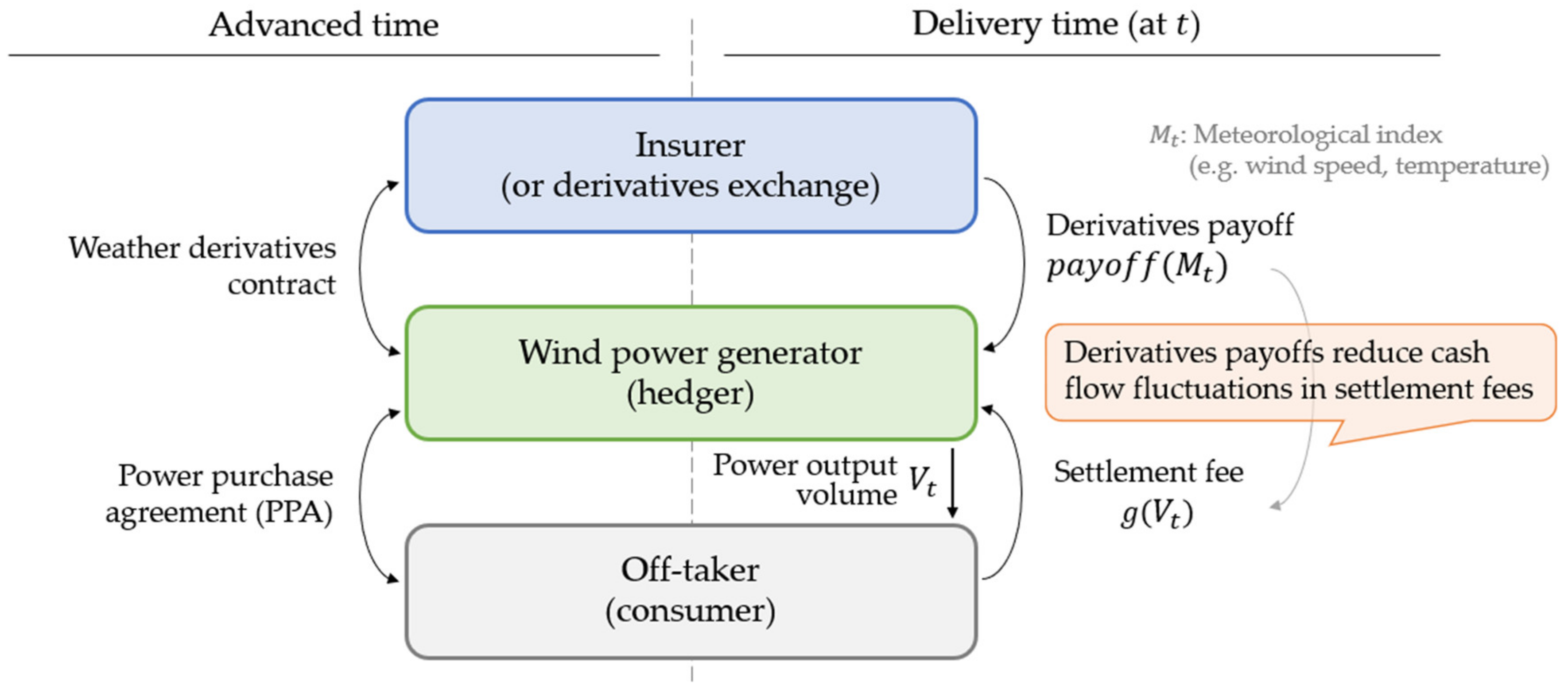
2.1. Market Trading Model

We first develop a market model and discuss possible trading schemes for the proposed weather derivatives. The overall picture of the transaction envisioned in this study is illustrated in Figure 1. Assume that a wind power generator sells the electricity to an off-taker under a power purchase agreement (PPA). The generator enters into a derivative contract with an insurance company (or purchases derivatives on an exchange market) in advance to hedge the risk of fluctuations in future electricity sales. Then, at delivery time t , the generator delivers the volume of power output V t to the off-taker and receives (or pays if negative) a cash flow g V t each time as a settlement fee, where the function g · is predetermined in the PPA. At the same time, due to the pre-contracted weather derivatives, the power generator receives p a y o f f M t that depends on the meteorological index (calculated from the observed values) M t ( M t may include wind speed, temperature, etc., and the function p a y o f f · is predetermined when the derivatives contract), and the generator’s loss is compensated to some extent. In this manner, the power generator can mitigate the risk of cash flow fluctuations.
In designing such weather derivatives, this study deals with two types of derivatives: non-parametric (made-to-order) and standardized derivatives. Figure 2 and Figure 3 provide a conceptual comparison of both derivative schemes, focusing on the market trading models and payoff functions (with the problem to be solved), respectively. Non-parametric derivatives use a bilateral contractual form where each hedger seeks an individual optimal derivative payoff, and both the seller and buyer agree with the transaction. Meanwhile, in the derivative trading scheme of our interest, the seller (i.e., an insurance company) can offer derivatives with standardized payoff functions (i.e., monomials of the weather indexes as the payoff functions) to any buyer, whereas buyers may agree to purchase them and include them in their portfolio. The buyer should choose the types and trading volumes of derivatives based on their own generation patterns and their correlation with the weather indices used. This standardization will allow hedgers (buyers) to trade only those instruments that are necessary according to their own risk tolerance. In addition, unlike non-parametric derivatives where payoffs are determined on a made-to-order basis, standardized derivatives allow multiple players to trade individual products. Similarly, if a sufficient number of sellers sell standardized derivatives, the market principle will help in better and fairer price discovery, and simultaneously many players may participate; this can increase the liquidity of the market. Furthermore, this study also proposes a way to use LASSO regression for decision-making on how to select effective derivative products to be traded in the market (or which and how much products hedgers should trade from the available products) in such a standardized derivatives market trading scheme, as will be discussed in detail in Section 2.5.
Additionally, instead of setting the insurance company as a potential seller, a more efficient trading scheme can be assuming that baseload power generators (who sell baseload power generation in the wholesale market) are the sellers of derivatives (risk underwriters). This is because when the derivatives’ payout is higher (i.e., when wind generation is lower), the baseload generator’s revenue from the wholesale power price also tends to be higher because of the reduced power supply, thereby conveniently offsetting cash flows. (For example, Ketterer [33] showed logically and empirically that an increase (decrease) in the supply of wind power affects the decrease (increase) in electricity prices.) In this transaction scheme, an insurance company can serve as an intermediary rather than a simple seller. Indeed, studies have considered similar schemes [34] for electricity, temperature, and/or solar radiation derivatives. Here, we focus on standardized schemes that are highly applicable to such transactions and that enhance liquidity market trading.
Note non-parametric derivatives are based on smoothing splines whereas standardized derivatives are based on (normal) polynomials, as will be discussed in detail in the next section. The difference is that the former is expressed using a smoothing spline function consisting of highly flexible piecewise (local) polynomials and is estimated by a GAM, a type of non-parametric regression (more precisely, it is expressed as a linear sum of multiple basis functions; see, e.g., [19] for the specific formulas). On the other hand, the latter is represented by a limited number of monomial-type functions. In other words, the former derivatives with payoffs represented by myriad polynomials do not fit into standardization, and to distinguish them from monomial-type standardized derivatives, we refer to them as non-parametric derivatives for convenience.

2.2. Minimum Variance Hedging Problem

In this study, we assume that the hedged risk is only the volume of wind power generated, and we do not consider price risk. Hedging volume risk in electric business is a challenging issue because it is generally difficult to completely hedge [7], and this is why several recent studies, especially in the renewable energy business, have often addressed the hedging problem for volume risk only [5,14,17,35]. These studies suggest that even if price risk is excluded (i.e., even if price risk can be completely hedged), weather derivatives are still effective because the volume risk of renewable energy is heavily linked to weather-related indices. With this in mind, we particularly consider the problem of mitigating cash flow fluctuations derived from power generation variations using derivative payoffs on wind speed and temperature. For example, if the hedger (wind power producer that generates V t at time t ) has a fixed-rate and fixed-quantity supply obligation contract in advance, where any shortage or surplus from the supply obligation amount v is settled at a fixed unit price θ , the profit and loss function to be hedged (i.e., g V t in Figure 1) is θ V t v . Note that this situation of assuming only volume risk corresponds to a power producer that has concluded a PPA with a general contract structure called “pay-as-produced,” and PPAs have been rapidly increasing in recent years as a new alternative to the conventional FITs [36].
Then, the minimum variance hedging problem defined below can be modeled without loss of generality by simply setting the hedge target to the generation volume V t . In this hedging problem (for a detailed exposition, see [34]), the hedger’s primary aim is to minimize the variance of the net cash flows of the electricity sales revenue (wind power generation volume) V t and the derivative payoff, p a y o f f W t ,   T t , composed of wind speed index W t and temperature index T t at each point in time:
minimize :   Var V t p a y o f f W t ,   T t
where the term p a y o f f W t ,   T t refers to the payoff function for non-parametric derivatives or the net payoff of the derivative portfolio in our standardized derivative scheme. The latter corresponds to the problem of finding the “contract volume” of standardized derivatives (detailed in the next subsections). Note that the units of each term in Equation (1) are currencies (e.g., EUR), but in this study, which compares among hedging models (to be constructed in the next and subsequent sections), the conversion of units and scales is not considered because it does not affect the results of the analyses. For example, when the unit price of electricity generation is θ , the payoff function of either model estimated is simply multiplied by θ , and the same results (e.g., hedge effect, which will be discussed later) will be obtained. Note also that Equation (1) has a degree of freedom with respect to the payoff’s location (first-order moment); therefore, it is possible to impose constraints on the mean value. For example, if a zero-mean constraint is imposed on the payoff itself (i.e., p a y o f f W t ,   T t ¯ = 0 ), it can be designed as a derivative with zero expected payoff without requiring an initial payment (or a premium) at contract time.

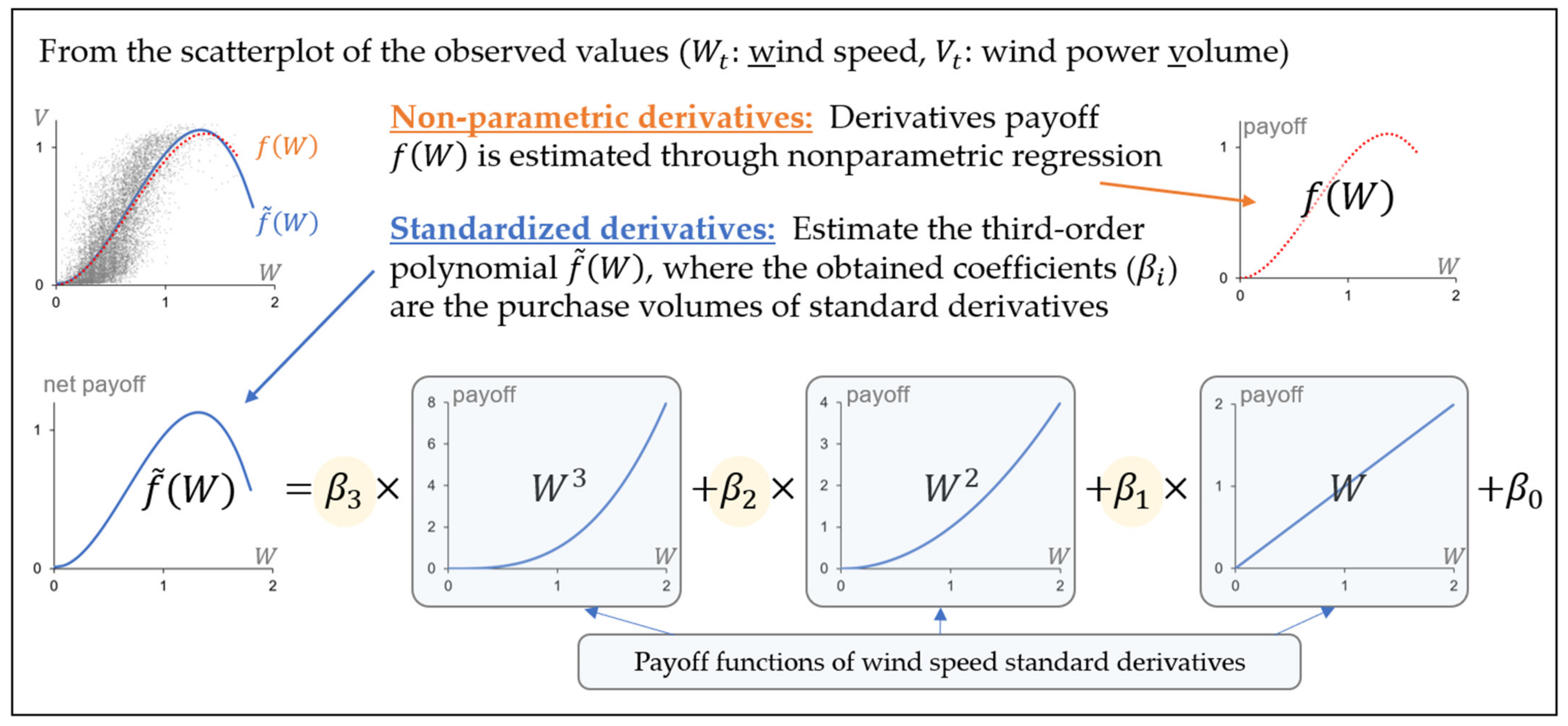
2.3. Non-Parametric Derivatives

In the case of the minimum variance hedging problem with non-parametric derivatives, the problem of optimizing the derivatives’ “payoff function” p a y o f f W t ,   T t f W t ,   T t in Equation (1) corresponds to estimating the following GAM:
V t = f W t ,   T t + ε t
where f is the two-dimensional tensor-product spline function [20] and ε t is the residual with a mean of 0. Because the estimation of GAM involves minimizing the sum of squares of the residual ε t under the smoothing constraint on f , it is synonymous with the variance minimization in Equation (1). Note that in this study, the GAM is estimated using the function gam() in the R package “mgcv” [20].
It is possible to design a “prediction error derivative” (i.e., a derivative with weather prediction errors as the underlying index) by removing the time-dependent trend from the underlying weather index (see, for example, [18]). However, we take an approach that does not remove the time-dependent trend from the underlying index, prioritizing the intuitive and straightforward cross-trend estimation of wind speed and temperature (e.g., the estimated payoff function shown in Section 3.1).

2.4. Standardized Derivatives

Next, in the case of minimum variance hedging problem with standardized derivatives, the problem is to optimize “contract/trading volume” of standardized derivatives based on the idea for approximating the payoff functions of non-parametric derivatives, f W t ,   T t , using simple multivariate polynomials denoted by f ˜ W t ,   T t . We consider the following model:
V t = f ˜ W t ,   T t + ε t ,           f ˜ W t ,   T t : = 0 i I ,   0 j J β i j W t i T t j
where W t i T t j i = 0 , I ;   j = 0 , , J are the payoff functions for different standardized derivatives. By estimating Equation (3) using OLS, hedgers can estimate the optimal (in the context of minimum variance hedging) contract volume β i j for each standardized derivative. Note that when i , j = 0 is a constant, the term can be regarded as a discount bond (with purchase unit β 00 ).
To consider the sufficient orders of derivatives, previous findings on wind power models are helpful (see Appendix A). Wind power output is generally modeled using a third-order formula for the wind speed [37]. In addition, wind turbines tend to reduce their power output when the temperature becomes too hot or too cold owing to a decrease in air pressure or freezing of components. This suggests an inverse U-shaped relationship with respect to temperature (see, e.g., https://www.windturbinestar.com/wind-turbine-annual-output.html, accessed on 15 June 2022). Based on the above considerations, this study adopts I = 3 and J = 2 in the hedging model in Equation (3). Note that the validity of assuming a nonlinear model was also verified by Ramsey’s RESET test [38] using our empirical data (see Appendix B).
Note also that because the average of the observed values with respect to W t and T t is positive, simply using the payoffs of second- or higher-order derivatives (i.e., when i or j is greater than 2) as powers of the observed values may cause unnecessary large variations in W t i or T t j . To avoid this problem, we design the initial (i.e., first-order) underlying indexes by subtracting the historical average from the observed value in advance; that is, W t W o b s ,   t W o b s ,   t ¯ , T t T o b s ,   t T o b s ,   t ¯ . This helps us in making derivatives more manageable and in increasing trading efficiency. The specific mechanism is discussed later (particularly in detail in Appendix D) using empirical data.
A recent study [26] has also shown that when designing hourly wind derivatives, wind speed derivatives at not only the same hour but also an hour before and after are effective. To apply this to our standardized derivative design, we set the wind speed index at each hour as a three-hour average value, including an hour before (lagged) and after (forward). That is, together with the above correction, the wind speed index used here is defined as follows: W t 1 / 3 τ = t 1 τ = t + 1 W o b s ,   τ W o b s ,   τ ¯ .

2.5. Hedge Trading Strategy Using LASSO Regression

The more incorporated the standardized derivatives are, the better replicated the nonlinear payoffs can be. However, using too many of them may reduce the out-of-sample period fit (i.e., hedge effect) due to overfitting. In addition, unnecessarily trading multiple derivatives may lead to trading inefficiencies in the form of increased product management costs or monitoring costs in the derivatives market. Similarly, reducing trading volume may be more desirable for efficient hedging strategies (see Appendix C for this discussion). Therefore, the strategy for estimating Equation (3) with the LASSO regression [39] may be more effective and efficient. It should be noted that, when dealing with conventional hedging problems, the standard OLS regressions were often applied for estimating hedging models since only a limited number of (existing) hedging instruments were mainly considered in the previous study. However, in this study, which introduces a market scheme for multiple derivatives that can be customized for a variety of hedgers, the use of LASSO regression should be particularly effective to ensure robustness and to improve trading efficiency (choice of trading instruments).
In LASSO regressions, the residual sum of squares with the L1 norm constraint on the regression coefficient vector is minimized. That is, each coefficient β is obtained as a solution to the following optimization problem using the regularization parameter λ :
minimize :   t = 1 T V t 0 i I ,   0 j J β i j W t i T t j 2 + λ 0 i I ,   0 j J β i j
Solving (4) allows us to reduce or eliminate less relevant variables [39]. That is, the LASSO regression will help sellers of derivatives (insurers or exchanges) identify products that are inherently in high need. On the other side for the buyers, it would be more efficient if they could select only the necessary (effective) derivatives while considering their risk tolerance and reduce the volume of each derivative. Note that when estimating the LASSO regression, it is desirable to standardize variables (i.e., “z-score” normalization) to provide equivalent penalties for variables with different units; this is also followed in this study. We estimate the LASSO regressions using the R package “glmnet,” where standardization of variables before model estimation and rescaling of coefficients after estimation are automatically performed as default settings [40,41].
For the regularization parameter λ , some values may be specified in advance. However, the cross-validation (CV) approach is an effective rational selection method. The most common way is to select the λ that minimizes the mean CV error ( λ m i n ); another method is to use the “one-standard error rule” (1SE rule: λ 1 s e ). Hastie et al. [40] defined the 1SE rule as a method to choose the most parsimonious model (i.e., the largest λ ), whose error is no more than one standard error above the error of the minimized error model, and suggested using the 1SE rule to select the best model. That is, the 1SE rule allows us to select the simplest model with the same accuracy as the best one [42]. Here, the adoption of this 1SE rule may help us in estimating a more efficient derivatives portfolio; that is, a portfolio with sufficient hedge effect while narrowing down the required number (or volume) of trading instruments as much as possible. Hence, our empirical analysis tests the effectiveness of trading strategies with LASSO regression by using both λ m i n and λ 1 s e , as well as by varying λ continuously.

3. Results

Next, we present the results of estimating the payoff function and calculating the hedge effect. Here, we use the following observed values of wind power generation and weather in Denmark, where wind power is very prevalent.
The estimation (in-sample) and validation periods (out-of-sample) are 2019 and 2020, respectively, using hourly data for all 24 h days from January 1 to December 31. The estimated trends and trading volumes (coefficients) were obtained from the in-sample period data only, whereas the hedge effects were calculated using the out-of-sample period data. Note that this study used data through 2020, which were available at the time the data were obtained, but as of the time of this paper’s submission, the data, including the most recent period, were no longer available to the public on that site.
Considering that sufficient historical data are often not available in practical situations, we estimated the hedge models from only one-year of in-sample data and calculated the hedge effect for the following year; this also helps in checking the robustness of the proposed method. Specifically, the hedge effect uses the variance reduction ratio (VRR) as 1 VRR . VRR is defined as follows:
VRR : = Var V t p a y o f f W t ,   T t / Var V t

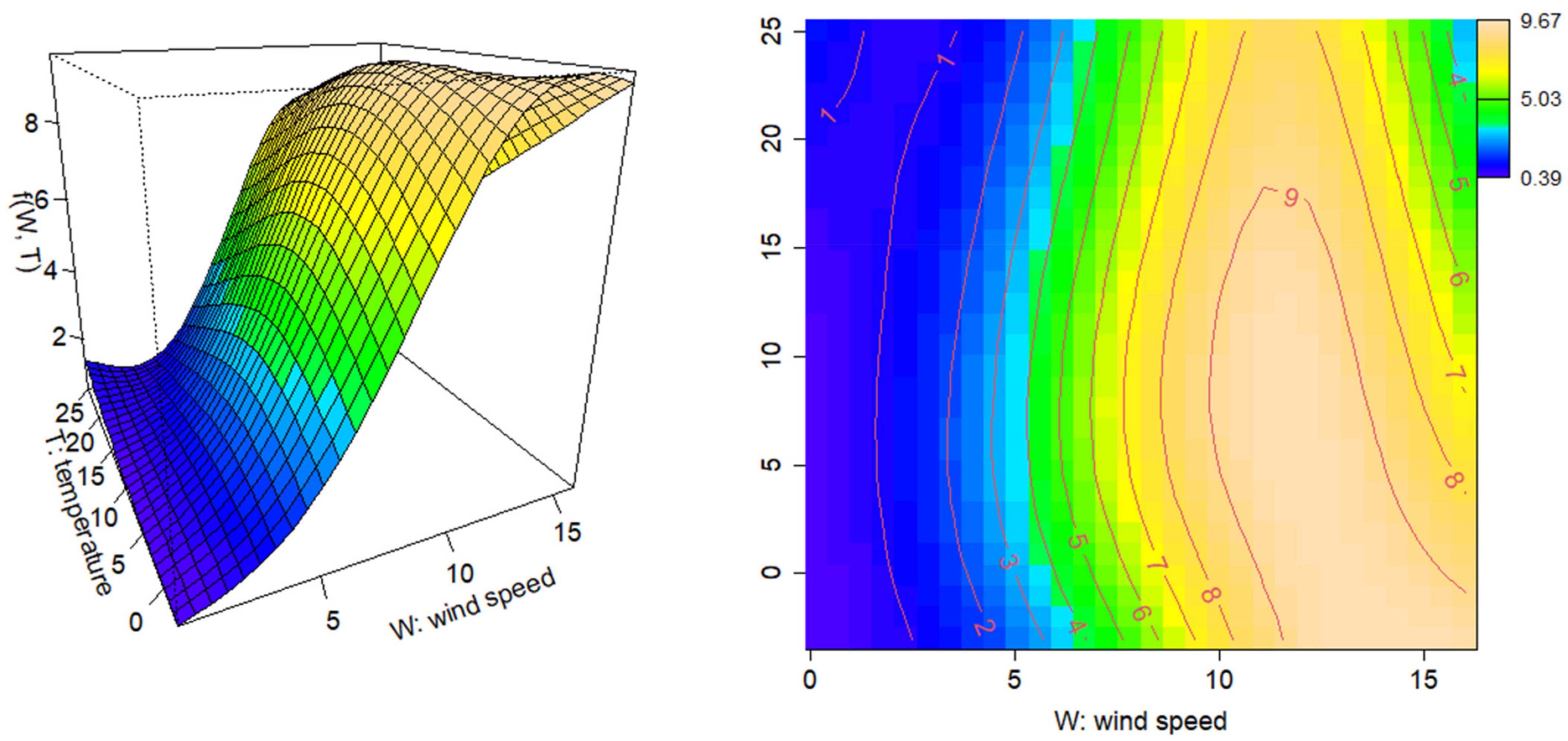
3.1. Estimated Trend (Non-Parametric Derivatives)

The trend of the estimated non-parametric derivative (i.e., f W t ,   T t in Equation (2)) is shown in Figure 4. As mentioned in Section 2.3, a cubic form in the wind speed direction and a near-quadratic form in the temperature direction were observed. For example, the sensitivity of wind power generation to wind speed was low when the wind speed was low, then increased as the wind speed increased, and finally decreased when the wind speed became too high. Meanwhile, the effect of temperature peaked at approximately 5–10 °C, and the power generation decreased at both higher and lower temperatures.

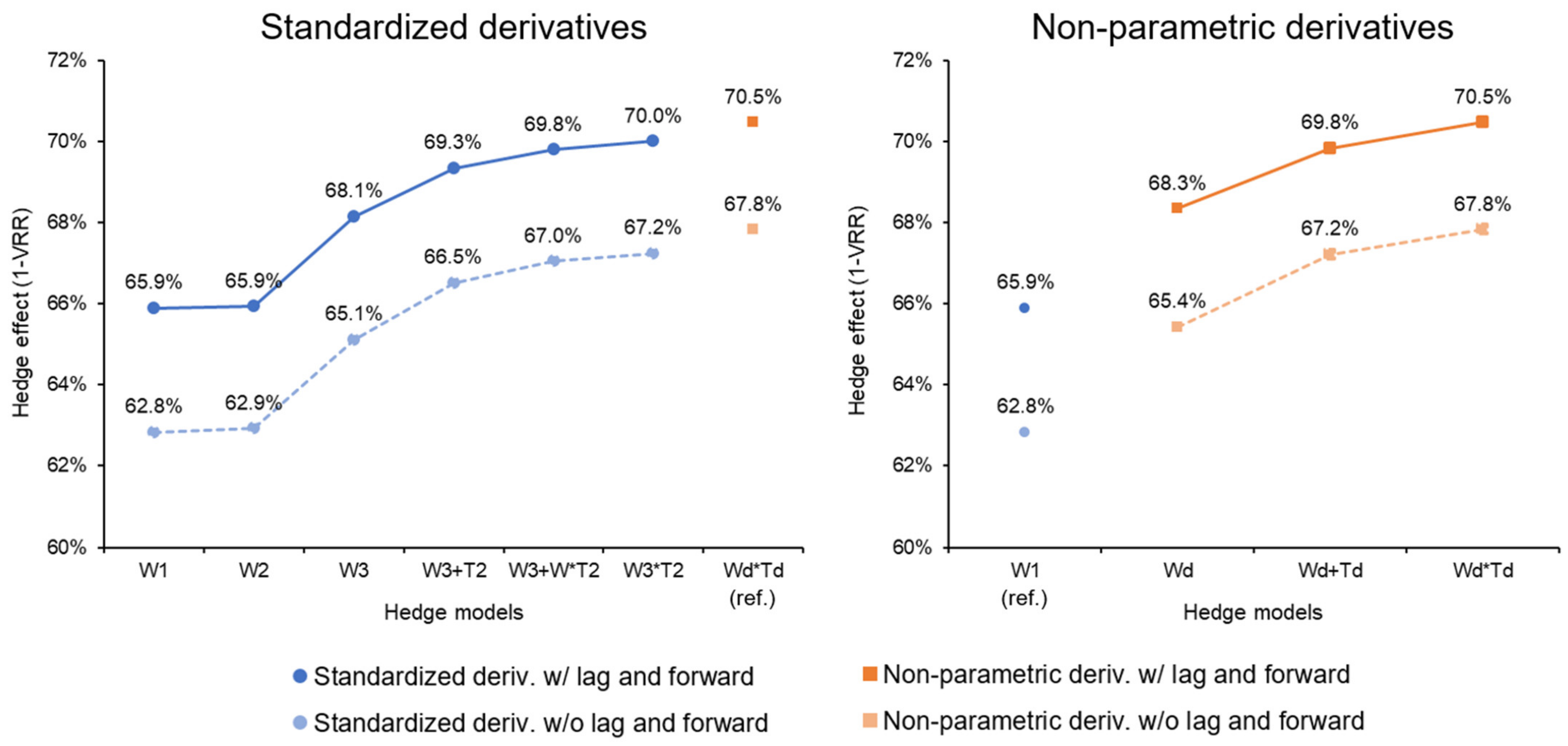
3.2. Measurement of Hedge Effects

Figure 5 plots the cumulative hedge effect, and the hedging products included in each hedging model are shown in Table 1 (note that the operators “+” and “*” are not strictly defined but are used for convenience to correspond intuitively with the long regression equation). The blue (orange) dots indicate the hedge effect of standardized (non-parametric) derivatives. For reference, the light blue and light orange dots are plotted together, showing the case where wind speeds before (lag) and after (forward) one hour are not included in the underlying indexes, as described in Section 2.4. Evidently, including wind speeds at the before and after hours in the underlying index is effective for improving the hedge effects; almost 3% improvements are observed in all hedging models.
Next, for both non-parametric and standardized types, the hedge effects increasd as the number of derivative combinations increased (i.e., the number of non-linear degrees of freedom increased). The hedge effect of using only “wind speed forwards” (W1) was 65.9%, while including “wind speed cubic derivatives” (W3) improved the hedge effect to 68.1% (68.3% for wind speed non-parametric derivatives). For the wind-speed squared derivative (W2), no improvement was observed in the hedge effect when combined with wind speed forwards without wind speed cubic derivatives, indicating that both derivatives are meaningful only when used in combination. The effect of temperature standardized derivatives was similar. The hedge effect can be increased to 69.3% when the “temperature squared derivative” is included (69.8% when temperature non-parametric derivatives are used) and 70% when all “wind speed and temperature cross-derivatives” are included (70.5% when the two-dimensional non-parametric derivative of wind speed and temperature is used).
For confirmation, the actual wind power generation versus payoffs of the derivative portfolio in the W3*T2 model is plotted in Figure 6. Because the payoff of the derivatives may be thought of as the predicted wind power generation (assuming that wind speed and temperature were observed), Figure 6 can be viewed as a fitting plot considering Equation (3) as a forecast model. Notably, the fluctuations of the two were generally consistent, except when power generation was extremely high/low. The wind speed and temperature indices are based on data observed at only one location (Copenhagen Airport); the model’s accuracy may improve by refining the indices.
The results of the above hedge effects are similar, even when viewed by month, as shown in Table 2. Notably, the effect of the “wind speed cubic derivative” improves the hedge effect in most months, and in some months, by more than 10% (e.g., 10.6% in March and 64.2% in August) compared to the case where only wind speed forward was used. While the hedge effect decreased in a few months, this decrease was limited.
The improvement in the hedge effect of “wind speed and temperature cross-derivatives” is particularly pronounced in the summer months. This may be due to the temperature variable successfully explaining the relationship between the continuous decrease in generation output (generation efficiency) with increasing temperature during the summer months, and hence the increased effectiveness of the temperature (cross) derivatives. In particular, August had the strongest non-linearity and interaction; the hedge effect improved by 114.6% when the temperature cross derivatives were included. Thus, the temperature-related derivatives do affect the reduction of wind turbine output (cash flow loss) due to high temperatures. Therefore, applying temperature derivatives or wind speed/temperature cross-derivatives especially for the summer months may provide useful hedges.

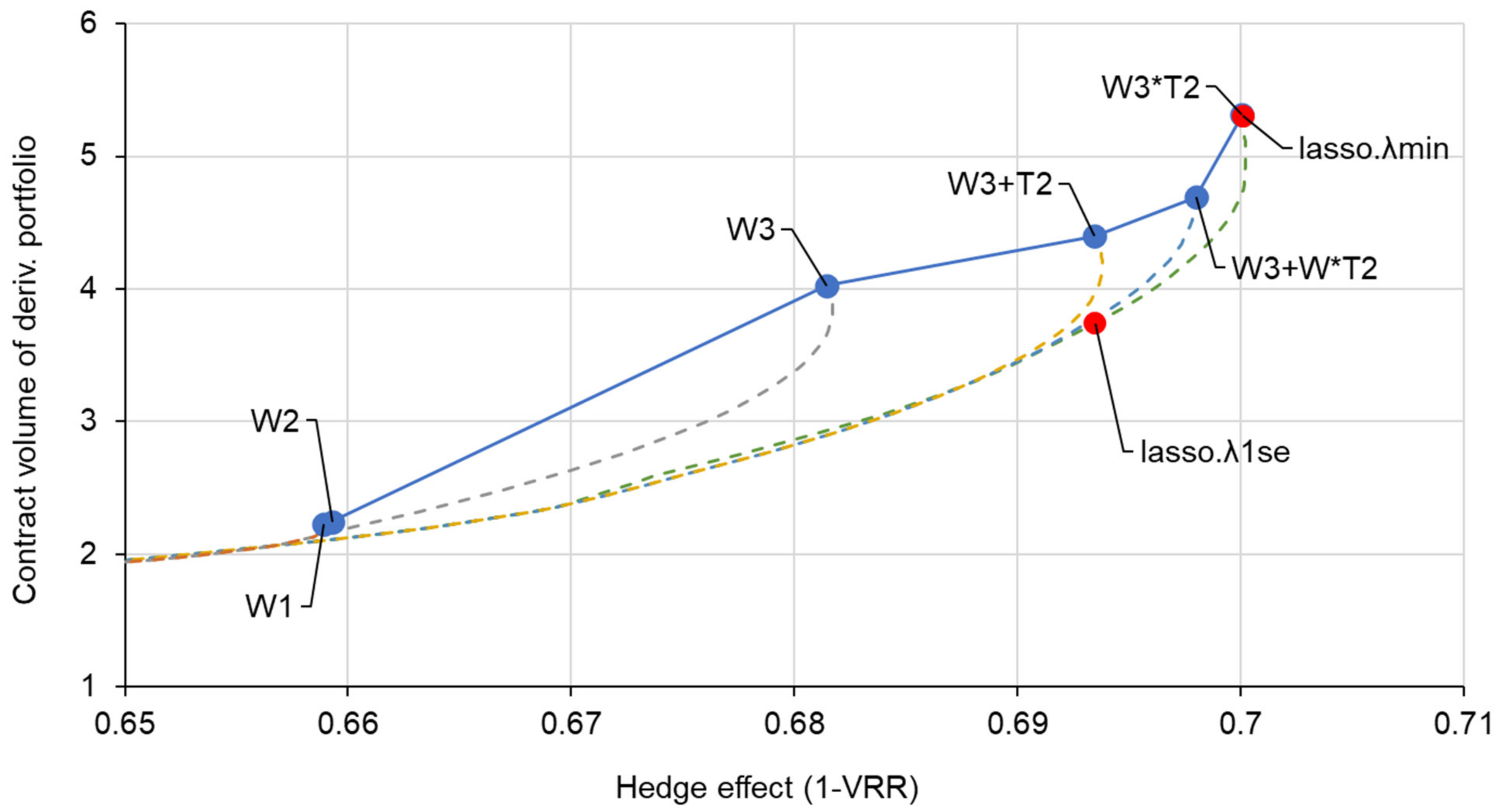
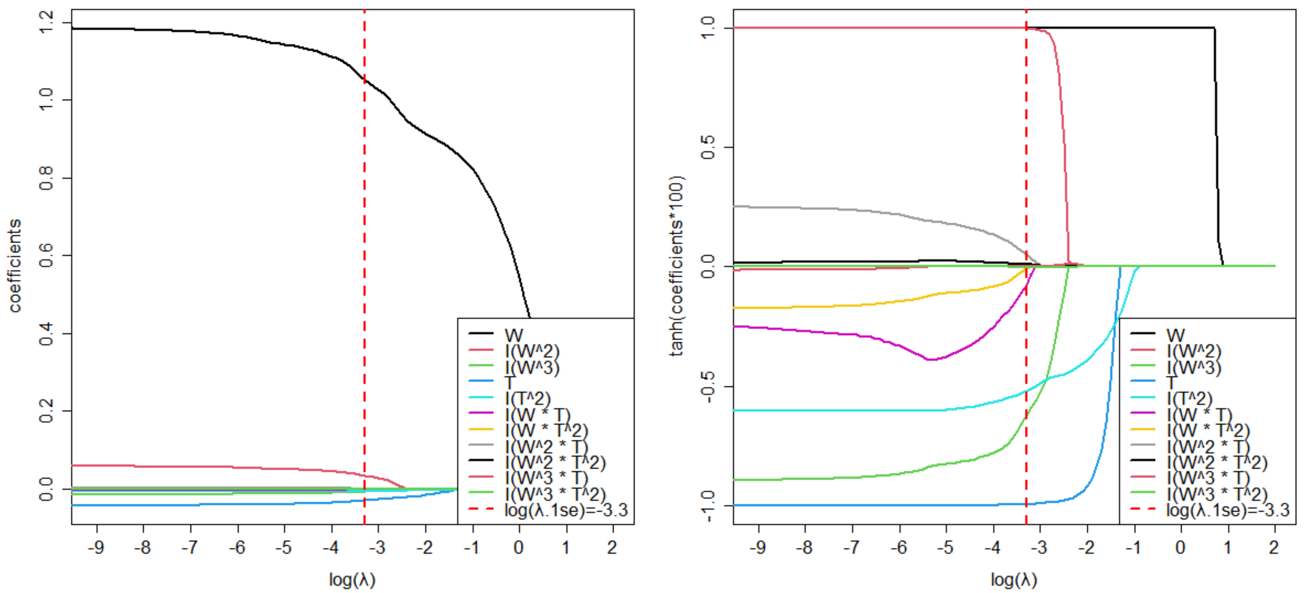
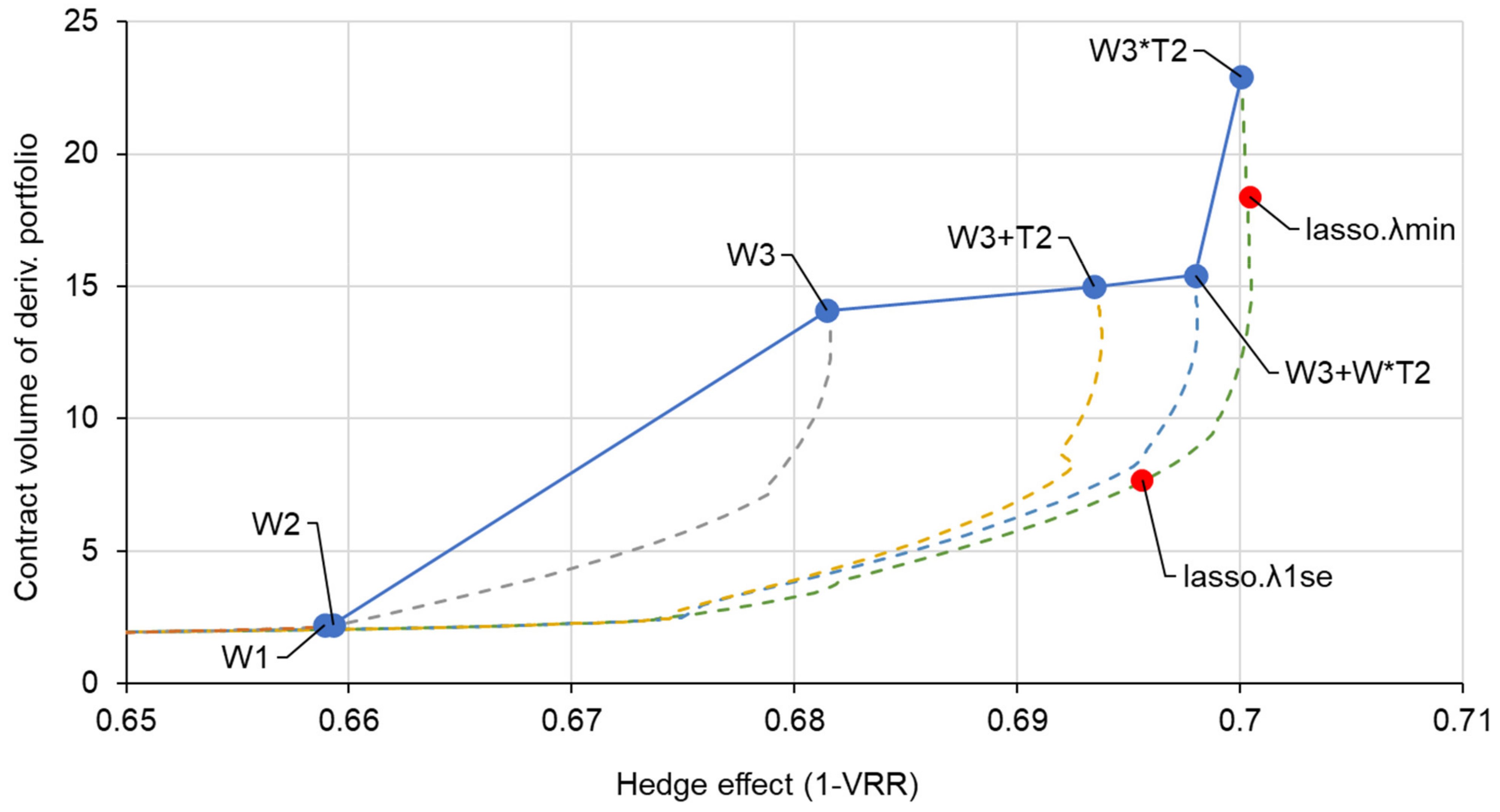
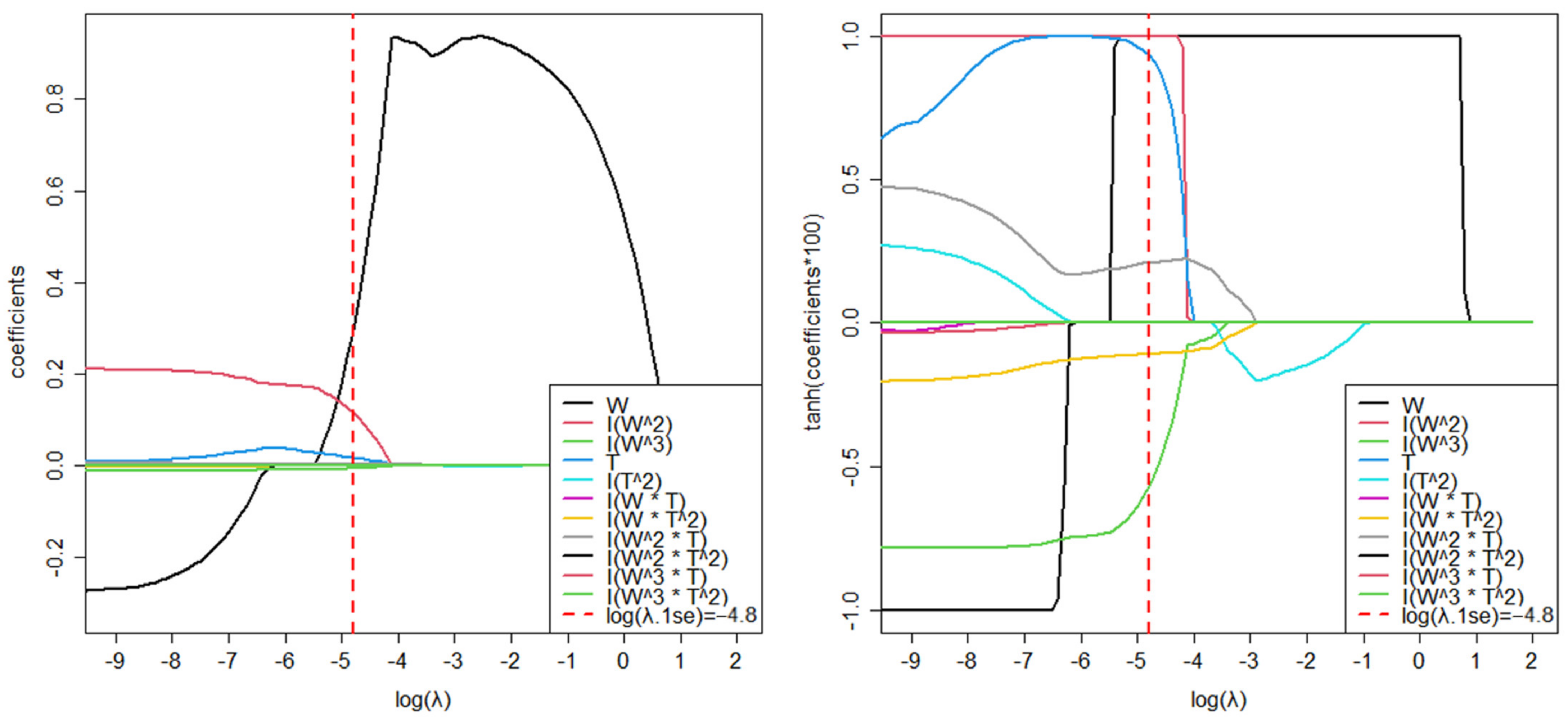
3.3. Trading Efficiency Using LASSO Regression

Finally, we tested the effectiveness of the “trading product selection” strategy of the LASSO regression described in Section 2.3. This strategy seems particularly effective when one intends to trade multiple standardized derivatives. Therefore, here, we take the “W3*T2” model (with an original hedge effect of 70.0%) as an example and estimate this model with a LASSO regression instead of the normal OLS. The regularization parameter λ in the LASSO regression is treated in two ways, λ m i n and λ 1 s e , as described in Section 2.5.
The contract/trading volumes (i.e., absolute values of the coefficients of the explanatory variables) for each derivative estimated by this method, including other hedging models using standardized derivatives, are shown in Table 3. The hedge effects shown in Figure 5 are also described at the bottom of the table. First, comparing the W3*T2 model with the models estimated using the LASSO regression, the hedge effect decreased slightly (by one percentage point) to 69.3% when using Lasso- λ 1 s e and remained virtually unchanged from the original 70.0% when using Lasso- λ m i n . However, there are notable differences in the product selection and volumes of trading, as discussed below.
First, regarding the product selection, we see that the trading volume of W 3 T was zero when Lasso- λ 1 s e is used. This is because the L1 regularization term in LASSO, explained in Section 2.5, reduced the variable’s coefficient (trading volume of the instrument) with the lowest contribution to 0. Note that increasing λ just a bit more makes it possible to further reduce the volume of multiple instruments traded to zero, which is discussed in detail later with a figure at the very end of this section.
In assessing trading volume, we examine not only the “simple sum” of the total trading volume of the derivatives portfolio but also a “weighted sum” weighted by the standard deviation of the payoffs of the individual derivatives. Note that the “weighted sum” is a useful measure of overall trading inefficiency, considering that hedge trading-related costs, such as the risk premium that a seller may demand, can depend on the instrument’s volatility (see Appendix C for more details). In both cases, the total volumes of the derivatives portfolio with LASSO are significantly smaller than those with regular OLS. For instance, the weighted sum using Lasso- λ 1 s e decreased from 5.31 to 3.74, a reduction of approximately 30%.
To verify the effectiveness of the LASSO regression to control trading volume, including the other hedging models (i.e., from W1 to W3+W*T2 models), we plot the relationship between contract volume and the hedge effect using the hedging model in Figure 7; here, the weighted sum in Table 3 is used as the trading volume on the vertical axis. First, as shown by the blue line, the trading volume increased with each additional product type, and simultaneously the hedge effect also increased. This result is consistent with practical intuition, as it suggests a trade-off exists between the hedge effect and its cost. However, the results of the trading strategies in the LASSO regression are more interesting. In Figure 7, they are drawn as dashed curves extending from the plot of each hedging model (i.e., the blue points where the trading volume is estimated by OLS, corresponding to λ = 0 ) to the lower left as λ gradually increases. Notably, the trading strategy estimated by LASSO for the W3*T2 model is generally below the line drawn by other models. That is, the strategy of using LASSO to estimate the trading volume of all derivatives (including higher-order derivatives) creates a “Pareto optimal” portfolio. Furthermore, the “Pareto optimal” frontier extends downward as the number of product types increases. This suggests that the availability of multiple instruments (i.e., trading multiple hedge products) not only increases the hedge effect but also contributes to reducing the hedger’s trading volume. For example, a portfolio with the W3 model (using wind speed derivatives only) would be an effective solution to increase the hedge effect as much as possible in a situation where no temperature-related derivatives were available. However, if temperature derivatives can be traded, one can construct a more efficient mixed portfolio in which only the trading volume can be noticeably reduced with the same hedge effect.
Note that the above analysis results are for the case where the hedging model is estimated using one year of in-sample data for 2019, as stated at the beginning of Section 3. Here, in order to verify the robustness of the results, as reference scenarios, we also calculated the results when using (A) two years of data for 2018–2019 and (B) half a year of data for July-December 2019, as the in-sample period. The pairs of {hedge effect, contract volume (weighted sum)} for the Lasso- λ 1 s e strategy were calculated to be {0.692, 3.819} for Case (A) and {0.682, 3.528} for Case (B). In both cases, the hedge effects were smaller than that of the benchmark case using one year of in-sample data, i.e., 0.693. Even when viewed in a two-dimensional plot that takes into account the trading volume, points A and B are inside the efficient frontier shown in Figure 7. The reason for this may be that taking too long of a learning period has the disadvantage of increasing the impact of changes in generation patterns due to renewal or expansion of generation facilities, while taking too short of a learning period makes robust estimation difficult. In general, for one-year ahead hedging, the use of the most recent one-year in-sample period, as adopted for the benchmark case, is considered appropriate from the perspective of ensuring a hedge effect.
For reference, Figure 8 shows the path diagram of the coefficients when the W3*T2 model is estimated by the LASSO regression with respect to the regularization parameter λ . Notably, increasing λ generally reduces the absolute value of each coefficient (i.e., the volume of each derivative contract). Further, each coefficient shrinks to zero as λ increases owing to the L1-norm penalty of the LASSO regression. If large transaction costs arise depending on the types of products traded (e.g., monitoring costs of price changes by product), then the decision of increasing λ can be made with reference to this path diagram to reduce the number of product types. For example, from the red vertical line in Figure 7, which represents λ 1 s e , some product types can be excluded from the portfolio by adjusting λ to slightly larger values. In any case, if λ is set too large, the coefficients (derivative volume) converge to zero and the hedge effect shrinks. Overall, to construct an efficient portfolio without impairing the hedge effect, the use of the 1SE rule λ is well balanced, as demonstrated above, and may provide an excellent criterion in the hedger’s decision-making process for the trading strategy.

4. Conclusions

This study demonstrated the effectiveness of hedging strategies using portfolios of high-order standardized weather derivatives applied to the wind power generation business. Our main contributions are as follows. First, we proposed new high-order monomial-type standardized derivatives, such as wind speed cubic derivatives and wind speed/temperature cross-derivatives, and demonstrated their effectiveness. Second, while developing a specific market trading scheme, we also showed the practical benefits of standardizing weather derivatives. Third, we proposed a “trading product selection” strategy using LASSO regression and demonstrated its effectiveness in terms of both increasing the efficiency of hedge trading and ensuring the hedge effect. Finally, we visualized the latent mixed trend in wind power generation relative to temperature and wind speed, and we noted the implications in the context of wind power forecasting models.
Essentially, we have shown that the hedge effect can be enhanced by incorporating various underlying hedge instruments and increasing the non-linearity of the portfolio. In particular, our new implication is that constructing a standardized derivatives portfolio is significant not only in hedge effect but also in hedge efficiency. By providing a variety of standardized hedging instruments, insurance companies (or exchanges) can give hedgers more flexible options for building their derivative portfolios. Estimating hedging models using LASSO regressions can help insurers/exchanges make decisions to identify efficient instruments. In addition, if hedgers adopt a trading strategy of LASSO regression, they can find and construct more Pareto-optimal portfolios, which help deal with the trade-off of reducing trading volume (transaction costs) and improving the hedge effect. Importantly, this mechanism may have generalizable implications for risk management practices in other businesses.
The primary idea provided by this study is in the original market scheme using new standardized derivatives for granular risk hedging, which would be increasingly needed in future decentralized electricity markets. Although relatively simple statistical methods such as OLS and LASSO regression were used for the methodology, our approach should have an advantage from the standpoint of practicality and applicability to the real world, i.e., a market scheme on methodologies that are as simple and straightforward as possible are superior. As a first step to examine the potential use of new higher-order standard derivatives, this study deals only with volume risk, but it would be interesting to examine the possibility of simultaneous hedging with price risk, which should be addressed in the future. In addition, the perspective of this research can be versatile, for example, in building a derivatives market for the distributed solar power generation business. The research questions for such applications may include verifying the effectiveness at daily granularity and further refining the hedging model by taking seasonality into account. Furthermore, from the perspective of further reducing transaction costs, methods other than LASSO regression could be used. LASSO regression has the advantage of reducing the number of hedge products due to its ability to shrink the coefficients of variables to zero, but if the costs associated with transaction volume (e.g., risk premiums) are more pronounced than the costs associated with the number of products (e.g., monitoring costs), other regularized regression methods, such as Ridge regression, might be superior. Further investigation of such questions may also be a subject for future work.
Derivatives with finer granularity and more variety, such as those addressed here, may have more demand once infrastructure, such as peer-to-peer power trading platforms, is in place. For instance, a fully digital trading platform will most likely reduce transaction costs. Moreover, a platform based on promising blockchain technology can enable immediate settlement or payment. (For example, the EnergyWeb blockchain has been developed for the energy sector and uses the “Proof-of-Authority” consensus algorithm. This blockchain has transaction rates hundreds to thousands of times higher than the “Proof-of-Work” conventional algorithm used by Bitcoin and other crypto applications, and it allows for instantaneous settlement [43].) Granular derivatives can be particularly useful for small players who wish to minimize fluctuations in their digital wallets. In any case, with the diversification of power resources, the increasing variety of hedging needs is an emerging trend. Then, naturally, hedging products should also be diversified. Given such future changes, the market design concept of diversification of hedging instruments and efficient trading scheme, as presented in this study, could be a potential basic idea to realize the decentralized power trading that will be needed in the future. Design methodologies, standardization schemes, and trading strategies for refined weather derivatives, such as those proposed here, may have useful implications in the electricity market, where transaction granularity is becoming increasingly finer in space and time.

Author Contributions

Conceptualization, T.M. and Y.Y.; methodology, T.M. and Y.Y.; software, T.M.; validation, T.M.; data curation, T.M.; writing—original draft preparation, T.M.; writing—review and editing, Y.Y.; visualization, T.M.; supervision, Y.Y.; project administration, Y.Y.; funding acquisition, T.M. and Y.Y. All authors have read and agreed to the published version of the manuscript.

Funding

Grant-in-Aid for Scientific Research (A) 20H00285, Grant-in-Aid for Challenging Research (Exploratory) 19K22024, and Grant-in-Aid for Young Scientists 21K14374 from the Japan Society for the Promotion of Science (JSPS).

Institutional Review Board Statement

Not applicable.

Informed Consent Statement

Not applicable.

Data Availability Statement

All data used in this study were obtained from the following websites: https://www.nordpoolgroup.com/en/Market-data1 (accessed on 11 January 2021); http://rp5.ru/metar.php?metar=EKCH (accessed on 11 January 2021). Note that the publication of the data on the former website has been terminated as of the time of submission of this paper, but the data for the period covered in this study are available from the first author.

Acknowledgments

This paper is an extension of the one presented at ICEER 2022, and their proceedings are to appear in “Energy Reports” (see Matsumoto and Yamada (2023)). This work was supported by Grant-in-Aid for Scientific Research (A) 20H00285, Grant-in-Aid for Challenging Research (Exploratory) 19K22024, and Grant-in-Aid for Young Scientists 21K14374 from the Japan Society for the Promotion of Science (JSPS).

Conflicts of Interest

The authors declare no conflict of interest.

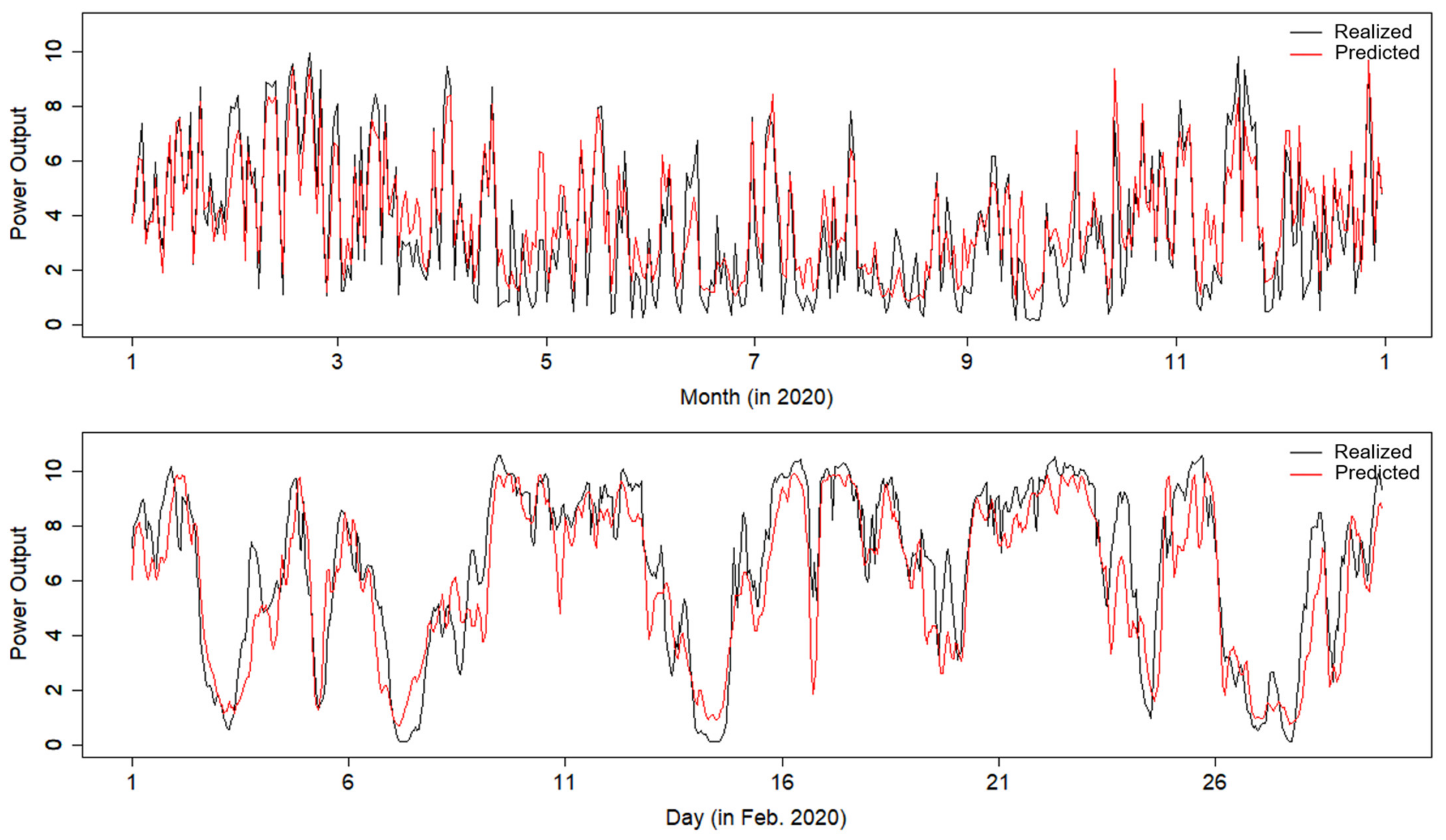
Appendix A. Research on Wind Power Output Forecasting

To develop an elaborate hedging model for wind power projects, we briefly reviewed studies on wind power forecasting. Broadly, wind power forecasting methods can be classified into time-series and exogenous variable models [44]. In recent years, the latter have emerged due to advances in computing technology and artificial intelligence, including several models that use machine learning (ML) methods such as artificial neural networks and deep learning [45]. Wind power generation is strongly correlated with wind speed, where intensity non-linearities exist. The relationship between wind turbine and wind speed has been analyzed in detail, focusing on technical characteristics; for example, in [46,47,48]. In general, the wind power curve is often described in the form of a cube of wind speed [37]. Marčiukaitis et al. [49] also compared and validated various models of non-linear regression with wind speed as an explanatory variable. Temperature is the next most commonly used explanatory variable after wind speed [45]. Some studies have demonstrated the effect of using temperature to improve accuracy using ML methods [50,51,52]; however, these studies do not clarify the structural effects of temperature and wind speed (including their interaction) on wind-power generation. Therefore, we intuitively illustrate the interaction between temperature and wind speed on wind power generation using a three-dimensional plot (Figure 4). This can provide useful insights in the context of wind power forecasting models.

Appendix B. Verification of Non-Linearity by Ramsey’s RESET Test

This study, which proposes the concept of trading schemes and strategies for high order standard derivatives, does not enter into the problem of optimizing the order of polynomial equations (3). That is, it is not the purpose of this study to determine whether third or second order is optimal as a power of wind speed or temperature. However, to verify the assumptions of the nonlinear models, Ramsey’s RESET test [38], a common test for linear regression, was performed on several models. In this test, the order of diagnostic variables for the linear function (null hypothesis) can be specified (see, for example, [53] as an empirical study), and the test was performed using the R package “lmtest” [54]. The results suggest the presence of strong nonlinearities, as shown in Table A1. In other words, it is worthwhile to use derivatives with higher-order monomial payoffs in combination with wind and temperature futures that have linear payoffs.
Table A1. The result of Ramsey’s RESET test.
ModelDiagnostic VariablesF-Statisticp-Value
V ~ Wsquares, cubes264.97 < 2.2 × 10 16
V ~ Tsquares305.21 < 2.2 × 10 16
V ~ W + Tsquares, cubes294.66 < 2.2 × 10 16
Note: this table is calculated using the function resettest() of the R package “lmtest” for the in-sample period data for Denmark presented in Section 3. “Model” is the “formula” of the original linear model and “Diagnostic variables” are the “power” of the fitted values of the linear model [54]. As the table shows, the p-values are essentially zero, meaning that the linear models of the null hypothesis are strongly rejected. For more information on this test, see, for example, “Chapter 9” in [55].

Appendix C. Hedge Trading Related Costs That Can Depend on Trading Volume

In general, an increase in hedging volume may result in an additional cost for a hedger from the following reasons. First, the bid/ask spread (BAS) is often used as a proxy for measuring the direct cost of transactions for market instruments [56]. Since a hedger must pay a BAS-equivalent transaction cost per trading (see, e.g., [57,58]), an increase in the trading volume leads to a rise in such a direct transaction cost. Another potential cost (which, in some cases, may be greater than the BAS) is the “risk premium” that the seller of a derivative contract adds to the selling price. The price of weather derivatives or derivatives (futures) in electricity markets is often formulated as the expected price of the underlying asset plus a risk premium (see, for example, [59] for weather derivatives and [60] for electricity futures), and the risk premium is interpreted as compensation for the seller’s risk burden (see, for example, [61,62]). That is, for the buyer, it corresponds to the cost of lowering his exposure [63]. Thus, curtailing the trading volume reduces this invisible cost corresponding to the risk premium.
In addition, both the BAS and the risk premium tend to increase as the volatility of the asset increases. For example, it has been demonstrated that there is a positive correlation between volatility and BAS [64,65] and volatility and risk premium [66] in various futures markets. In other words, the values calculated in Section 3.3, where the trading volume is weighted by the standard deviation of the payoffs of each instrument, have a certain rationality as an indicator of hedge trading related costs.

Appendix D. The Case of Using Derivatives with No Average Value Correction for the Underlying Index

In Section 2.4, we noted that when designing higher-order standardized derivatives, it is desirable to subtract the mean from the first-order underlying (we refer to this case as a “corrected case”); here, we show the reason for this. First, if such a correction is not made (an “uncorrected case”), the volatility of higher-order derivatives will be unnecessarily large, which will worsen the efficiency of the transaction. Figure 7 in Section 3.3, shows the relationship between trading volume (“weighted sum” considering standard deviation) and hedge effect for the “corrected” derivatives; the corresponding plot for the “uncorrected” case is shown in Figure A1 below. While the absence of the correction has little effect on the hedge effects as they are perfectly consistent in the ordinary least squares (OLS) estimation case, the standard deviation-weighted trading volumes (trading costs) are several times larger than those shown in Figure 7. Although the least absolute shrinkage and selection operator (LASSO) regression strategy is effective in reducing trading volume in this uncorrected case as well (the volume is reduced to approximately 1/3 using the 1SE rule), the volume can be reduced much more when using corrected derivatives. Specifically, even with the 1SE rule, trading volume decreased to 3.74 in the corrected case, while it only decreased to 7.68 in the uncorrected case.
Figure A1. Relationship between contract volume and hedge effect by hedging model (cases in which no mean value correction was made for the underlying indexes). Note: the term “lasso” refers to the W3*T2 model estimated by LASSO regression. Hedge effect is measured in out-of-sample periods. Note: the blue dots represent the estimation results from OLS and the dashed curves represent the estimation results obtained by varying λ in the LASSO regression.
Energies 16 03112 g0a1
The path diagram of the estimated coefficients (derivative volume) from the LASSO regression for the uncorrected case is also shown in Figure A2 (for comparison, see Figure 8 for the corrected case). Note that the coefficients are not stable with respect to the moving λ . For example, the hedger’s position in wind futures has changed significantly from a sell position to zero position and then to a buy position as λ increases. Further, the paths of the other coefficients are also generally not smooth. This is irrational from the perspective of efficient decision making in trading practice. In addition, assuming, for example, that this derivative supported continuous trading, such an unstable volume path can lead to unnecessary rebalancing of trading positions. This is not desirable from a transaction-cost perspective.
Figure A2. Relationship between the regularization parameter λ and the coefficients in LASSO regression (i.e., cases with no mean value correction for the underlying indexes). The graph on the right transforms the scale of the left graph using the hyperbolic tangent function ( t a n h 100 x ) for ease of viewing.
Energies 16 03112 g0a2

References

  1. IEA. Renewables 2021 Analysis and Forecast to 2026. Available online: https://www.iea.org/reports/renewables-2021 (accessed on 15 June 2022).
  2. Market Research Future. Small Wind Power Market. Available online: https://www.marketresearchfuture.com/reports/small-wind-power-market-4568 (accessed on 15 June 2022).
  3. Botterud, A.; Wang, J.; Bessa, R.; Keko, H.; Miranda, V. Risk management and optimal bidding for a wind power producer. In IEEE PES General Meeting; IEEE: Minneapolis, MN, USA, 2010; pp. 1–8. [Google Scholar] [CrossRef]
  4. Bathurst, G.; Weatherill, J.; Strbac, G. Trading wind generation in short term energy markets. IEEE Trans. Power Syst. 2002, 17, 782–789. [Google Scholar] [CrossRef]
  5. Yamada, Y. Optimal Hedging of Prediction Errors Using Prediction Errors. Asia-Pacific Financ. Mark. 2008, 15, 67–95. [Google Scholar] [CrossRef] [Green Version]
  6. Eydeland, A.; Wolyniec, K. Energy and Power Risk Management: New Developments in Modeling, Pricing, and Hedging; John Wiley & Sons: Hoboken, NJ, USA, 2002; Volume 97. [Google Scholar]
  7. Deng, S.; Oren, S. Electricity derivatives and risk management. Energy 2006, 31, 940–953. [Google Scholar] [CrossRef]
  8. Benth, F.E.; Pircalabu, A. A non-Gaussian Ornstein–Uhlenbeck model for pricing wind power futures. Appl. Math. Financ. 2018, 25, 36–65. [Google Scholar] [CrossRef] [Green Version]
  9. Gersema, G.; Wozabal, D. An equilibrium pricing model for wind power futures. Energy Econ. 2017, 65, 64–74. [Google Scholar] [CrossRef]
  10. Benth, F.E.; Di Persio, L.; Lavagnini, S. Stochastic Modeling of Wind Derivatives in Energy Markets. Risks 2018, 6, 56. [Google Scholar] [CrossRef] [Green Version]
  11. Rodríguez, Y.; Pérez-Uribe, M.; Contreras, J. Wind Put Barrier Options Pricing Based on the Nordix Index. Energies 2021, 14, 1177. [Google Scholar] [CrossRef]
  12. Kanamura, T.; Homann, L.; Prokopczuk, M. Pricing analysis of wind power derivatives for renewable energy risk management. Appl. Energy 2021, 304, 117827. [Google Scholar] [CrossRef]
  13. Christensen, T.S.; Pircalabu, A. On the spatial hedging effectiveness of German wind power futures for wind power generators. J. Energy Mark. 2018, 11, 71–96. [Google Scholar] [CrossRef]
  14. Masala, G.; Micocci, M.; Rizk, A. Hedging Wind Power Risk Exposure through Weather Derivatives. Energies 2022, 15, 1343. [Google Scholar] [CrossRef]
  15. Hastie, T.; Tibshirani, R. Generalized Additive Models; Chapman & Hall: Boca Raton, FL, USA, 1990. [Google Scholar]
  16. Yamada, Y. Valuation and hedging of weather derivatives on monthly average temperature. J. Risk 2007, 10, 101–125. [Google Scholar] [CrossRef] [Green Version]
  17. Matsumoto, T.; Yamada, Y. Cross Hedging Using Prediction Error Weather Derivatives for Loss of Solar Output Prediction Errors in Electricity Market. Asia-Pacific Financ. Mark. 2018, 26, 211–227. [Google Scholar] [CrossRef]
  18. Matsumoto, T.; Yamada, Y. Simultaneous hedging strategy for price and volume risks in electricity businesses using energy and weather derivatives. Energy Econ. 2021, 95, 105101. [Google Scholar] [CrossRef]
  19. Matsumoto, T.; Yamada, Y. Customized yet Standardized Temperature Derivatives: A Non-Parametric Approach with Suitable Basis Selection for Ensuring Robustness. Energies 2021, 14, 3351. [Google Scholar] [CrossRef]
  20. Wood, S.N. Generalized Additive Models: An Introduction with R; Chapman and Hall: New York, NY, USA, 2017. [Google Scholar]
  21. Oum, Y.; Oren, S.; Deng, S. Hedging quantity risks with standard power options in a competitive wholesale electricity market. Nav. Res. Logist. 2006, 53, 697–712. [Google Scholar] [CrossRef]
  22. Oum, Y.; Oren, S.S. Optimal Static Hedging of Volumetric Risk in a Competitive Wholesale Electricity Market. Decis. Anal. 2010, 7, 107–122. [Google Scholar] [CrossRef] [Green Version]
  23. Brik, R.I.; Roncoroni, A. Static mitigation of volumetric risk. J. Energy Mark. 2016, 9, 111–150. [Google Scholar] [CrossRef]
  24. Carr, P.; Madan, D. Optimal positioning in derivative securities. Quant. Financ. 2001, 1, 19–37. [Google Scholar] [CrossRef]
  25. Matsumoto, T.; Yamada, Y. Multivariate Weather Derivatives for Wind Power Risk Management: Standardization Scheme and Trading Strategy. Energy Rep. 2023, in press. [Google Scholar]
  26. Yamada, Y.; Matsumoto, T. Construction of Mixed Derivatives Strategy for Wind Power Producers; University of Tsukuba: Tokyo, Japan, 2023; manuscript in preparation. [Google Scholar]
  27. Ederington, L.H. The hedging performance of the new futures markets. J. Financ. 1979, 34, 157–170. [Google Scholar] [CrossRef]
  28. Zainudin, A.D.; Mohamad, A. Cross hedging with stock index futures. Q. Rev. Econ. Finance 2021, 82, 128–144. [Google Scholar] [CrossRef]
  29. Ong, T.S.; Tan, W.F.; Teh, B.H. Hedging effectiveness of crude palm oil futures market in Malaysia. World Appl. Sci. J. 2012, 19, 556–565. [Google Scholar]
  30. Woo, C.-K.; Horowitz, I.; Hoang, K. Cross hedging and forward-contract pricing of electricity. Energy Econ. 2001, 23, 1–15. [Google Scholar] [CrossRef]
  31. Sant’Anna, L.R.; Caldeira, J.F.; Filomena, T.P. Lasso-based index tracking and statistical arbitrage long-short strategies. N. Am. J. Econ. Finance 2020, 51, 101055. [Google Scholar] [CrossRef] [Green Version]
  32. Chen, Q.-A.; Hu, Q.; Yang, H.; Qi, K. A kind of new time-weighted nonnegative lasso index-tracking model and its application. N. Am. J. Econ. Financ. 2022, 59, 101603. [Google Scholar] [CrossRef]
  33. Ketterer, J.C. The impact of wind power generation on the electricity price in Germany. Energy Econ. 2014, 44, 270–280. [Google Scholar] [CrossRef] [Green Version]
  34. Yamada, Y.; Matsumoto, T. Going for Derivatives or Forwards? Minimizing Cashflow Fluctuations of Electricity Transactions on Power Markets. Energies 2021, 14, 7311. [Google Scholar] [CrossRef]
  35. Mosquera-López, S.; Uribe, J.M. Pricing the risk due to weather conditions in small variable renewable energy projects. Appl. Energy 2022, 322, 119476. [Google Scholar] [CrossRef]
  36. RE-Source. Risk Mitigation for Corporate Renewable PPAs. 2017. Available online: https://resource-platform.eu/wp-content/uploads/files/statements/RE-Source%203.pdf (accessed on 3 February 2022).
  37. Ko, W.; Hur, D.; Park, J.-K. Correction of wind power forecasting by considering wind speed forecast error. J. Int. Counc. Electr. Eng. 2015, 5, 47–50. [Google Scholar] [CrossRef] [Green Version]
  38. Ramsey, J.B. Tests for Specification Errors in Classical Linear Least-Squares Regression Analysis. J. R. Stat. Soc. Ser. B (Methodol.) 1969, 31, 350–371. [Google Scholar] [CrossRef]
  39. Tibshirani, R. Regression Shrinkage and Selection Via the Lasso. J. R. Stat. Soc. Ser. B 1996, 58, 267–288. [Google Scholar] [CrossRef]
  40. Hastie, T.; Tibshirani, R.; Friedman, J.H.; Friedman, J.H. The Elements of Statistical Learning: Data Mining, Inference, and Prediction; Springer: New York, NY, USA, 2009; Volume 2, pp. 1–758. [Google Scholar]
  41. Friedman, J.; Hastie, T.; Tibshirani, R.; Narasimhan, B.; Tay, K.; Simon, N.; Qian, J. Package ‘glmnet’. CRAN R Repositary. Available online: https://cran.r-project.org/web/packages/glmnet/index.html (accessed on 15 June 2022).
  42. Krstajic, D.; Buturovic, L.J.; Leahy, D.E.; Thomas, S. Cross-validation pitfalls when selecting and assessing regression and classification models. J. Cheminform. 2014, 6, 10. [Google Scholar] [CrossRef] [PubMed] [Green Version]
  43. Alladi, T.; Chamola, V.; Rodrigues, J.J.P.C.; Kozlov, S.A. Blockchain in Smart Grids: A Review on Different Use Cases. Sensors 2019, 19, 4862. [Google Scholar] [CrossRef] [PubMed] [Green Version]
  44. Foley, A.M.; Leahy, P.G.; Marvuglia, A.; McKeogh, E.J. Current methods and advances in forecasting of wind power generation. Renew. Energy 2012, 37, 1–8. [Google Scholar] [CrossRef] [Green Version]
  45. Hanifi, S.; Liu, X.; Lin, Z.; Lotfian, S. A Critical Review of Wind Power Forecasting Methods—Past, Present and Future. Energies 2020, 13, 3764. [Google Scholar] [CrossRef]
  46. Chaurasiya, P.K.; Kumar, V.K.; Warudkar, V.; Ahmed, S. Evaluation of wind energy potential and estimation of wind turbine characteristics for two different sites. Int. J. Ambient Energy 2021, 42, 1409–1419. [Google Scholar] [CrossRef]
  47. Chaurasiya, P.K.; Ahmed, S.; Warudkar, V. Wind characteristics observation using Doppler-SODAR for wind energy applications. Resour.-Effic. Technol. 2017, 3, 495–505. [Google Scholar]
  48. Werapun, W.; Tirawanichakul, Y.; Waewsak, J. Wind shear coefficients and their effect on energy production. Energy Procedia 2017, 138, 1061–1066. [Google Scholar] [CrossRef]
  49. Marčiukaitis, M.; Žutautaitė, I.; Martišauskas, L.; Jokšas, B.; Gecevičius, G.; Sfetsos, A. Non-linear regression model for wind turbine power curve. Renew. Energy 2017, 113, 732–741. [Google Scholar] [CrossRef]
  50. Aksoy, B.; Selbaş, R. Estimation of Wind Turbine Energy Production Value by Using Machine Learning Algorithms and Development of Implementation Program. Energy Sources Part A Recover. Util. Environ. Eff. 2019, 43, 692–704. [Google Scholar] [CrossRef]
  51. Bilal, B.; Ndongo, M.; Adjallah, K.H.; Sava, A.; Kébé, C.M.; Ndiaye, P.A.; Sambou, V. Wind turbine power output prediction model design based on artificial neural networks and climatic spatiotemporal data. In Proceedings of the 2018 IEEE International Conference on Industrial Technology, Buenos Aires, Argentina, 26–28 February 2020; pp. 1085–1092. [Google Scholar]
  52. De Giorgi, M.G.; Ficarella, A.; Tarantino, M. Assessment of the benefits of numerical weather predictions in wind power forecasting based on statistical methods. Energy 2011, 36, 3968–3978. [Google Scholar] [CrossRef]
  53. Vaona, A. Spatial autocorrelation or model misspecification? The help from RESET and the curse of small samples. Lett. Spat. Resour. Sci. 2009, 2, 53–59. [Google Scholar] [CrossRef]
  54. Hothorn, T.; Zeileis, A.; Farebrother, R.W.; Cummins, C.; Millo, G.; Mitchell, D.; Zeileis, M.A. Package ‘lmtest’. Testing Linear Regression Models. Available online: https://cran.r-project.org/web/packages/lmtest/lmtest.pdf (accessed on 3 February 2023).
  55. Wooldridge, J.M. Introductory Econometrics: A Modern Approach; Cengage learning: Boston, MA, USA, 2015. [Google Scholar]
  56. Demsetz, H. The Cost of Transacting. Q. J. Econ. 1968, 82, 33–53. [Google Scholar] [CrossRef]
  57. Lobo, M.S.; Fazel, M.; Boyd, S. Portfolio optimization with linear and fixed transaction costs. Ann. Oper. Res. 2006, 152, 341–365. [Google Scholar] [CrossRef]
  58. Georgiev, K.; Kim, Y.S.; Stoyanov, S. Periodic portfolio revision with transaction costs. Math. Methods Oper. Res. (ZOR) 2015, 81, 337–359. [Google Scholar] [CrossRef]
  59. Chen, F.Y.; Yano, C.A. Improving Supply Chain Performance and Managing Risk Under Weather-Related Demand Uncertainty. Manag. Sci. 2010, 56, 1380–1397. [Google Scholar] [CrossRef] [Green Version]
  60. Bunn, D.W.; Chen, D. The forward premium in electricity futures. J. Empir. Financ. 2013, 23, 173–186. [Google Scholar] [CrossRef]
  61. Longstaff, F.A.; Wang, A.W. Electricity Forward Prices: A High-Frequency Empirical Analysis. J. Financ. 2004, 59, 1877–1900. [Google Scholar] [CrossRef] [Green Version]
  62. Gagliardini, P.; Ossola, E.; Scaillet, O. Time-Varying Risk Premium in Large Cross-Sectional Equity Data Sets. Econometrica 2016, 84, 985–1046. [Google Scholar] [CrossRef] [Green Version]
  63. Woodard, J. Options and the Volatility Risk Premium; Pearson Education: London, UK, 2011. [Google Scholar]
  64. Batchelor, R.A.; Alizadeh, A.H.; Visvikis, I.D. The relation between bid–ask spreads and price volatility in forward markets. Deriv. Use Trading Regul. 2005, 11, 105–125. [Google Scholar] [CrossRef]
  65. Bryant, H.L.; Haigh, M.S. Bid–ask spreads in commodity futures markets. Appl. Financ. Econ. 2004, 14, 923–936. [Google Scholar] [CrossRef]
  66. Yoo, J.; Maddala, G.S. Risk premia and price volatility in futures markets. J. Futur. Mark. 1991, 11, 165–177. [Google Scholar] [CrossRef]
Figure 1. Overall picture of the transactions assumed in this study (from derivatives contracts to settlements).
Energies 16 03112 g001
Figure 2. Market trading model for wind derivatives. Note: “W” represents wind speed index and “T” represents temperature index.
Energies 16 03112 g002
Figure 3. Conceptual diagram of methods for determining standardized (non-parametric) derivatives’ trading volume (payoff functions). Note: this conceptual diagram is an example of using only wind speed derivatives.
Energies 16 03112 g003
Figure 4. Estimated trends of non-parametric derivatives (left: perspective, right: contour).
Energies 16 03112 g004
Figure 5. Hedge effects of standardized derivatives and non-parametric derivatives.
Energies 16 03112 g005
Figure 6. Realized versus predicted values of wind power generation in the out-of-sample period (Upper: 2020, Lower: February 2020). Note: the upper graph plots daily averaged values for visibility. The realized data are the raw wind production data downloaded from https://www.nordpoolgroup.com/en/Market-data1/ (accessed on 11 January 2021).
Energies 16 03112 g006
Figure 7. Relationship between contract volume and hedge effect by hedging model. Note: the term “lasso” refers to the W3*T2 model estimated by LASSO regression. Hedge effect is measured in out-of-sample periods. Note: the blue dots represent the estimation results from OLS and the dashed curves represent the estimation results obtained by varying λ in the LASSO regression.
Energies 16 03112 g007
Figure 8. Relationship between the regularization parameter λ and the coefficients in LASSO regression. The graph on the right transforms the scale of the left graph using the hyperbolic tangent function ( t a n h 100 x ) for ease of viewing.
Energies 16 03112 g008
Table 1. Components of hedging instruments by hedging model.
Standardized Derivatives ModelNon-Parametric Derivatives Model
W1W2W3W3+T2W3+W*T2W3*T2WdWd+TdWd*Td
Standardized derivatives W
W 2
W 3
T + T 2
W T + W T 2
W 2 T + W 2 T 2 + W 3 T + W 3 T 2
Non-parametric derivatives f W W
f T T
f t e W ,   T
Table 2. Monthly hedge effect and improvement rate against the W1 model.
Monthly Hedge EffectAll
Period
JanFebMarAprMayJunJulAugSepOctNovDec
Hedge effect
(1-VRR)
W168.6%76.1%65.4%59.1%58.7%40.9%66.3%15.4%63.5%62.8%72.8%60.9%65.9%
W367.5%79.4%72.3%59.9%59.5%43.9%69.1%25.3%68.8%62.5%75.9%60.3%68.1%
W3*T268.6%80.7%71.5%59.2%61.1%46.9%74.0%33.0%68.8%63.8%76.0%59.8%69.3%
Improvement rate (to “W1”)W3−1.6%4.4%10.6%1.4%1.4%7.2%4.3%64.2%8.3%−0.4%4.2%−1.1%3.4%
W3*T20.0%6.1%9.3%0.2%4.0%14.7%11.6%114.6%8.4%1.7%4.4%−1.8%5.2%
Note: improvement rate is the ratio of the increase in the hedge effect of each hedging model relative to that of the W1 model; the largest value among the models in each month for both hedge effect and improvement rate is shown in bold.
Table 3. Derivatives contract volume by hedging model, including LASSO regression-based trading strategies.
W1W2W3W3+T2W3+W*T2W3*T2 lasso . λ m i n lasso . λ 1 s e Stdev of Payoffs
Contract volumes of each derivative (absolute values of coefficients)
W0.984650.978951.139051.118141.161141.184861.184261.050632.3
I(W^2)-0.003780.069300.065410.062860.058670.058200.033678.3
I(W^3)--0.014060.013690.013760.014600.014550.0072862.3
T---0.033240.032830.042370.042440.030226.4
I(T^2)---0.005690.006130.006940.006970.0057946.3
I(W * T)----0.003550.002460.002290.0008013.8
I(W * T^2)----0.001130.001800.001770.00006128.2
I(W^2 * T)-----0.002580.002620.0005156.3
I(W^2 * T^2)-----0.000160.000170.00011428.9
I(W^3 * T)-----0.000150.00017.361.8
I(W^3 * T^2)-----0.000040.000040.000032651.4
Contract volumes of derivatives portfolio
Simple sum0.984650.982731.222411.236171.281401.314631.313481.12909
Weighted sum2.228052.246324.025854.400154.692295.312855.305543.74113
Hedge effects of derivatives portfolio
1-VRR0.658920.659290.681460.693430.697970.700060.700090.69348
Disclaimer/Publisher’s Note: The statements, opinions and data contained in all publications are solely those of the individual author(s) and contributor(s) and not of MDPI and/or the editor(s). MDPI and/or the editor(s) disclaim responsibility for any injury to people or property resulting from any ideas, methods, instructions or products referred to in the content.

