The Double Lanes Cell Transmission Model of Mixed Traffic Flow in Urban Intelligent Network

Abstract

The connected and autonomous vehicle (CAV) is promised to ease congestion in the future with the rapid development of related technologies in recent years. To explore the characteristics of mixed-traffic flow and the dynamic transmission mechanism, this paper firstly detailed the car-following model of different vehicle types, establishing the fundamental diagram of the mixed-traffic flow through considering the different penetration rates and fleet size of CAV. Secondly, this paper constructed the lane-changing judgment mechanism based on the random utility theory. Finally, the paper proposed a lane-level dynamic cell transmission process, combined with a lane-changing strategy and cell transmission model. The effectiveness and feasibility of the model are verified using simulation analysis. This model makes a systematic, theoretical analysis from the perspective of the internal operation mechanism of traffic flow, and the lane-level traffic strategy provides a theoretical basis for balancing urban lane distribution and intelligent traffic management and control.

1. Introduction

Urban traffic congestion will not only reduce the traffic efficiency and bring serious environmental pollution, but it will also threaten traffic safety. With the improvement of infrastructure construction, as well as the development of intelligent transportation technology and automatic driving technology, the dynamic characteristics between vehicles are greatly changed, altering the traditional traffic flow within inherent attributes. Therefore, the application of intelligent vehicles is generally accepted as a solution to the traffic congestion problem. However, universal access to intelligent vehicles will not happen overnight, in which case the mixed-traffic flow, composed of traditional human driving vehicles (HVs) and intelligent vehicles, will be normalized, which has made the mixed-traffic flow and dynamic transfer process become a hot spot of research at home and abroad.

Because of the quite different characteristics of traditional HVs and intelligent vehicles, Shladover [1] first took time headway into account in conducting a traffic simulation based on real driving data, studying the impact of adaptive cruise control (ACC) vehicles and cooperative adaptive cruise control (CACC) vehicles under different penetration rates on highway capacity, but there are no details for control strategy and contact between vehicles. Milanes [2] established a car-following model according to the corresponding characteristics of the vehicle longitudinal control system, verifying that CACC vehicles provide a stable chasing response through a small-scale, actual vehicle experiment. Hao Liu [3] constructed a model that accurately describes the behavior of CACC vehicles, reflecting the lane-changing rules based on the lane management and the traffic flow change of the complex road bottleneck area, under the control-mode-switching algorithm.

These studies are more inclined to start with the micro-behavior of individual vehicles, and explore the influence of individual traffic characteristic parameters of intelligent vehicles on traffic flow, without considering the interaction between vehicles. As intelligent vehicles can perceive the surrounding environment and interaction between vehicles through onboard units and roadside units, they have better environmental perception ability [4,5]. Therefore, vehicle formation control has become one of the key technologies of intelligent vehicles. Thus, the influence of intelligent fleets on traffic flow has attracted wide attention recently, including the influence of fleet organization, vehicle market penetration rate, fleet size, and intelligent assisted driving degree [6,7,8,9]. Different driving characteristics of intelligent vehicles and HVs reflect the obvious diversity of free traffic flow, so the mixed-traffic flow composing both of them will be evidently different from the traffic flow composed of the same kind of vehicles in the process of transmission. By analyzing the stability conditions of mixed-traffic flow under the different penetration rates of intelligent vehicles, the mixed-traffic flow fundamental diagram is used to reflect the influence of driving characteristics, such as minimum safe distance, expected headway interval, vehicle delay, and response time, on traffic capacity [10,11,12].

The mixed-traffic flow dynamic transfer mechanism still needs to be clarified. The car-following model is an important microscopic model of traffic flow, which scholars have conducted a lot of research work on that can be described by the optimal velocity (OV) model [13], generalized force (GF) model [14], full velocity difference (FVD) model [15], multiple velocity difference (MVD) model [16], and cellular automata (CA) model [17], etc. The lane-changing model is another kind of important microscopic traffic flow model. Scholars have widely used Gipps, Microscopic traffic simulator (MITSIM), and other models to describe it [18,19]. Recently, the fuzzy logic model, neural network model, and game theory model have been widely used with the rise of sensing technology and artificial intelligence technology [20,21,22,23]. However, the microscopic model has a small modeling scope, which makes it difficult to grasp the overall traffic impact and has low modeling efficiency, limiting the practical implement in urban areas. Compared with the micro-car-following modeling, there is relatively less research on the macro-modeling and meso-modeling of the traffic flow [24].

Using the gas dynamics theory, Ngoduy [25] proposed a macro model for describing the intelligent traffic flow dynamic, proving that CAV fleet can enhance traffic-flow stability in the on-ramp bottleneck area under small perturbations. Delis [26] introduced the relaxation factor, satisfying the space and time interval principle of ACC and CACC systems. Traffic flow will be considered a compressible continuous fluid medium composed of a large number of vehicles, studying the average behavior of the collective. In contrast, the macroscopic traffic-flow model characteristic for individuals is not explicit and is not fine enough to obtain and analyze the quantitative indicators of intersections.

Levin [27] proposed the mesoscopic traffic-flow model to predict the shock wave and road capacity while considering reaction time based on the cell transmission model (CTM). Tiaprasert [28] put forward the multiple-lane CTM to enhance the first-in, first-out (FIFO) character and transmission capacity of CTM, taking the priority of different level vehicles under congestion into account, but not refining the lane-changing strategy at lane level, weakening the possible conflict problem. Thus, the lane-level traffic management strategy based on the incentive of downstream condition is detailed [29], and the first-order lane level CTM was constructed while considering motivation function. While the results of this method are sensitive to the parameters of the traffic-flow fundamental diagram, it ignores the changes caused by the expected behavior of drivers. Namely, it did not show the characteristics of mixed-traffic flow.

To summarize, the existing research focuses more on improving the cell transmission model itself, and independently studies the microscopic driving behavior and macroscopic traffic flow characteristics under the intelligent network environment, which are treated as two separate systems. This paper expects to study them in combination, and build a meso-traffic flow transfer process that can reflect both microscopic car-following and lane-changing behaviors and macroscopic traffic flow analytical characteristics. As a connecting bridge, it can not only capture the discontinuous change of traffic flow, but also better connect with the road network model, which provides a new research idea for traffic dynamic assignment problems and shortens the research distance between road traffic flow and network traffic flow.

The overall structure of this paper is shown in Figure 1.

The structure of this paper is as follows. The second part describes the characteristic analysis of vehicles and considers the impact of penetrance rate and fleet distribution of CAVs on the fundamental diagram of mixed-traffic flow. The third part conducts the lane-changing judgment mechanism, which compares the profits between lanes. The fourth part builds a double-lane CTM, deducing the flow conservation equation count for profits and realizing the lane-level dynamic transmission between cells in intelligent networks. The fifth part is the simulation and the conclusion.

2. Research Methodology

In this paper, we detail the car-following model of different types of vehicles, which build the fundamental diagram of the mixed-traffic flow while considering the different penetration rates and fleet size of CAV. Random utility theory, applied to the lane-changing judgment mechanism combined with CTM, proposes a lane-level dynamic cell transmission process. Thus, the research methodology consists of driving characteristic analysis, along with lane-changing judgment mechanism and simulation analysis, of double-lane CTM.

2.1. The Analysis of Driving Characteristics

Traditional HV generally has no cooperation function. With the integration of intelligent connected technology and automatic driving technology, CAV arises at a historic moment [30]. Additionally, due to communication technology from vehicle to vehicle (V2V), speed, acceleration, distance, and other information can be updated in real time, running under the CACC pattern. When communication equipment is not loaded, the vehicles will run under the ACC pattern, named AV.

2.1.1. Car-Following Model

The Intelligent Driver Model (IDM) is regarded as the car-following behavior model of HV, and the PATH Laboratory of the University of California, Berkeley verified the ACC and CACC model-respecting car-following behavior model of AV and CAV.

• HV car-following model based on IDM

The IDM model is a widely recognized expectation measurement model not based on accident theory, assuming that the expected speed and headway remain constant in the driving process [31]. Due to the ignorance of reaction time at the same section of road on the same lanes in the mesoscopic model of the HV car-following model, as well as the IDM model with the real physical meaning of parameters, the calibrated parameter will be more accessible if it directly reflects the variation of HV driving behavior at the mesoscopic level. The specific expression is as follows:

$${\dot{v}}_{IDM}(t)=a[1-{(\frac{v(t)}{\tilde{v}})}^{\sigma }-{(\frac{\tilde{s}+T_{h}v(t)+\frac{v(t)\Delta v(t)}{2\sqrt{ab}}}{h(t)-l})}^2]$$

(1)

where ${\dot{v}}_{IDM}(t)$ is the acceleration at moment $t$, $v(t)$ is the speed at moment $t$, $\Delta v(t)$ is the difference between the vehicle and the front at moment $t$, $h(t)$ is the distance headway between the vehicle and the front at moment $t$, $\tilde{v}$ is the speed of free traffic flow, $\tilde{s}$ is the minimum safety distance, $a$ is the expected maximum acceleration, $b$ is the expected deceleration, $T_h$ is the expected safe time headway, $\sigma$ is the acceleration index, and $l$ is the length of the vehicle.

• AV car-following model based on ACC

AV monitors the distance from the vehicle in front in real time through radar, infrared sensor and other equipment, calculate the speed, acceleration and additional information of the vehicle in front, to adjust the driving characteristics of the vehicle itself and achieve the purpose of autonomous driving. The PATH Laboratory of the University of California, Berkeley has verified the ACC car-following model under the constant time headway strategy, which conforms to the real dynamic car-following character [7]. The specific expression is as follows:

$${\dot{v}}_{ACC}(t)=k_1[h(t)-T_{a}v(t)-l-\tilde{s}]+k_2\Delta v(t)$$

(2)

where ${\dot{v}}_{ACC}(t)$ is acceleration at moment $t$, $T_a$ is expected safe time headway, $k_1$ is control coefficient 1, $k_2$ is control coefficient 2.

• CAV car-following model based on CACC

Through V2V communication technology, CAVs continuously adjust the error term of actual and expected distance to control the change of the rear vehicle speed in real time, in which case has a shorter response time and a shorter time headway. The PATH laboratory also used real vehicle data to verify the CACC model under the proposed constant time headway strategy. The specific expression is as follows:

$$\left.\begin{array}{l}{v}_{CACC}(t+\Delta t)=v_p(t)+k_{p}e(t)+k_d\dot{e}(t)\begin{array}{c}\end{array}\\ e(t)=h(t)-\tilde{s}-l-T_{c}v(t)\end{array}\right\}$$

(3)

where $\Delta t$ is the control step, $v_{CACC}(t+\Delta t)$ is the speed at moment $t+\Delta t$, $v_p(t)$ is the speed at moment $t$, $e(t)$ is the error between actual and expected spacing at moment $t$, $\dot{e}(t)$ is the differential term of $e(t)$ with respect to $t$, $k_p$ is the control coefficient of vehicle spacing error; $k_d$ is the control coefficient of differential term of vehicle spacing error, $T_c$ is the expected safe time headway.

2.1.2. Vehicle Proportion Allocation

The CAVs realize the cooperative operation between vehicles. Still, when the front vehicle of CAV is not equipped with communication equipment, not satisfying the V2V communication conditions, the CAV at the rear vehicle position will degenerate into AV [32]. Therefore, the fundamental diagram of mixed-traffic flow constructed in this paper is based on the following assumptions:

• AV is only degenerated by CAV following HV.
• When CAV forms a fleet, only the first vehicle of the fleet degenerates to AV.
• The mesoscopic model IDM does not consider the response time of vehicles in the same lane of the same road section.

Suppose that in a fleet with $n$ vehicles, when penetration rate of intelligent vehicles is $p$, the penetration rate of CAV is $p_c$, the penetration rate of AV is $p_a(p_a+p_c=p)$, and the penetration rate of HV is $p_h=1-p$. If the size of the spontaneous CAV fleet is $n_c$, there will be $np/n_c$ CAV fleets on the road. Thus, the probability of a CAV fleet and HV on the road, $P_{CAV}$ and $P_{HV}$, are, respectively:

$$\left.\begin{array}{l}{P}_{CAV}=\frac{p/n_c}{p/n_c+(1-p)}\begin{array}{c}\end{array}\\ P_{HV}=\frac{1-p}{p/n_c+(1-p)}\end{array}\right\}$$

(4)

Then, the probability $P_{AV}$ of AV is:

$$P_{AV}=\frac{p/n_c}{p/n_c+(1-p)}\times \frac{1-p}{p/n_c+(1-p)}=\frac{n_{c}p(1-p)}{{[p+n_c(1-p)]}^2}$$

(5)

2.1.3. Analytical Expression of Traffic Flow

As CAV has the ability to spontaneously form a flexible fleet, there are mainly four forms in car-following situations including fleets: HV follows HV, HV follows CAV fleet, CAV fleet follows HV, and CAV fleet follows CAV fleet, and their proportion is respectively $P_{HV}{P}_{HV}$, $P_{HV}{P}_{CAV}$, $P_{CAV}{P}_{HV}$, $P_{CAV}{P}_{CAV}$.

Assuming the research scope is large enough, the total length of a single-lane road with n vehicles can be expressed as the sum of the equilibrium distance headways of all motorcades. In the mixed-traffic flow, the speed in the equilibrium state is identical. Still, due to different driving characters of CAV, AV, and HV, balanced-distance headways have various performances, and $h_c,h_a,h_h$ respectively represent the headways in CAV, AV, and HV equilibrium states. Therefore, the analytical formula of the density–flow fundamental diagram can be derived from the distance–headway–speed relationship of the equilibrium traffic flow. Distance headway $h$ of the mixed-traffic flow can be expressed as:

$$\begin{array}{l}h=\frac{p+n_c(1-p)}{n_c}\{P_{HV}{P}_{HV}{h}_h+P_{HV}{P}_{CAV}[(n_c-1)h_c+h_h]\\ \hspace{1em}\hspace{1em}\hspace{1em}\hspace{1em}\hspace{1em}\hspace{1em}\hspace{1em}+P_{CAV}{P}_{HV}[h_a+(n_c-1)h_c]+P_{CAV}{P}_{CAV}{n}_c{h}_c\}\end{array}$$

(6)

Then, distance headways of the balanced flow in Equations (1)–(3) are brought into Equation (6). The analytical expression of the mixed-traffic flow density–flow fundamental diagram, including fleet, is:

$$\left.\begin{array}{l}k=\{\frac{p+n_c(1-p)}{n_c}\{P_{HV}{P}_{HV}(\frac{\tilde{s}+T_h{v}_e}{\sqrt{1-{(v_e/\tilde{v})}^4}}+l)\\ \begin{array}{cccc}& & & \begin{array}{cc}& \end{array}\end{array}+P_{HV}{P}_{CAV}[(n_c-1)\left(T_c{v}_e+l+\tilde{s}\right)+(\frac{\tilde{s}+T_h{v}_e}{\sqrt{1-{(v_e/\tilde{v})}^4}}+l)]\begin{array}{c}\end{array}\\ \begin{array}{cccc}& & & \begin{array}{cc}& \end{array}\end{array}+P_{CAV}{P}_{HV}[(T_a{v}_e+l+\tilde{s})+(n_c-1)\left(T_c{v}_e+l+\tilde{s}\right)]\\ \begin{array}{cccc}& & & \begin{array}{cc}& \end{array}\end{array}+P_{CAV}{P}_{CAV}{n}_c\left(T_c{v}_e+l+\tilde{s}\right)\}{\}}^{-1}\\ \\ q=k{v}_e\end{array}\right\}$$

(7)

2.2. Lane-Changing Judgment Mechanism

Free lane changing occurs when guaranteed under the premise of safety and necessity, and predicting lane-changing behavior can earn expected benefits.

2.2.1. Random Utility Theory

For a set of alternative items that are independent of each other, it is believed that items with the most excellent utility will be selected, which is the basis of random-utility theory, called the utility maximization behavior hypothesis [33]. According to random utility theory, the conditions for travelers to select a candidate are:

$$U_i>U_j\begin{array}{cc}& \end{array}i\ne j\begin{array}{cc}& \end{array}i,j\in A$$

(8)

where, $U_i,U_j$ is the utility of candidate $i,j$, and $A$ is the set of all candidate options for travelers.

Each choice made by the candidate is random, so the candidate’s utility consists of fixed and random utility. For simplicity, suppose they are independent and linear, and expressed by the following equation:

$$\left.\begin{array}{l}{U}_i=V_i+{\alpha }_i\\ V_i={\beta }_0+{\displaystyle \sum _{n=1}^N{\beta }_n{X}_{in}\begin{array}{c}\end{array}}\end{array}\right\}$$

(9)

where, utility is composed of observable fixed utility $V_i$ and unobservable random term ${\alpha }_i$. Fixed utility $V_i$ that affects the selection is determined by a characteristic variable $X_{in}$, and ${\beta }_n$ is the coefficient of $X_{in}$, which is a constant. According to utility maximization theory, the probability of selecting a candidate $i$ is:

$$\begin{array}{ll}{P}_i& =\mathrm{Prob}(U_i>U_j;i\ne j;i,j\in A)\\ & =\mathrm{Prob}(V_i+{\alpha }_i>V_j+{\alpha }_j;i\ne j;i,j\in A)\end{array}$$

(10)

where $0\le P_i\le 1,{\displaystyle {\sum }_{i\in A}{P}_i}=1$.

When a random term ${\alpha }_i$ satisfies the same parameter and independent double exponential distribution, the multinomial logit model can be further expressed as:

$$P_i=\frac{\exp (V_i)}{{\displaystyle {\sum }_{j\in A}\exp (V_j)}}\begin{array}{cc}& \end{array}i\in A$$

(11)

2.2.2. Lane-Changing Revenue Model

In the mesoscopic traffic flow model, as shown in Figure 2a, the road is divided into sections of fixed length, and vehicles in each section have a certain probability of changing lanes, resulting in changes in the number of vehicles in different lanes. Thus, the profitability of the free lane-changing behavior is reflected in the difference between the driving benefits of the current road section and the adjacent road section. Because the target lane has more excellent driving conditions, drivers tend to change lanes in pursuit of a better driving environment. For the mesoscopic traffic flow model, the benefits of free lane-changing include time benefits and space benefits. The time benefit is reflected in obtaining more incredible average speed in the road section, and the time to pass the fixed-length section is correspondingly shorter. The space benefit is reflected in smaller average density in the road section, and a better field of vision to further quantify the revenue value of free lane changing. The following revenue model, which is based on random utility theory, is established.

Some vehicles may change lanes between different lanes in the adjacent road section. Using double lanes as an example, it can be abstracted as the situation shown in Figure 2b. Before entering the next section, vehicles can determine whether to change direction or keep going straight according to their current driving status.

Figure 2. The lane-changing scene of (a) mesoscopic traffic flow model, and (b) abstraction of double-lane traffic flow transfer.

Figure 2. The lane-changing scene of (a) mesoscopic traffic flow model, and (b) abstraction of double-lane traffic flow transfer.

where, when entering the next section $i+1$ from the current section $i$, $P_{11}$ is the probability of going straight from the current lane $L_1$, $P_{12}$ is the probability of changing lanes from the current lane $L_1$ to lane $L_2$, $P_{21}$ is the probability of changing lanes from the current lane $L_2$ to lane $L_1$, and $P_{22}$ is the probability of going straight from the existing lane $L_2$.

There are two choices for the vehicles in section $i$ of lane $L_1$: continue straight or change lanes. The probability is respectively:

$$\left.\begin{array}{l}{P}_{11}=\frac{\exp (V_{11})}{\exp (V_{11})+\exp (V_{12})}\\ P_{12}=\frac{\exp (V_{12})}{\exp (V_{11})+\exp (V_{12})}\begin{array}{c}\end{array}\end{array}\right\}$$

(12)

$V_{11}$ is the fixed utility of going straight in lane $L_1$, $V_{12}$ is the fixed utility of changing lanes from $L_1$ to $L_2$. Similarly, there are two choices for vehicles in section $i$ of lane $L_2$–continue straight or change lanes–with probability as follows:

$$\left.\begin{array}{l}{P}_{22}=\frac{\exp (V_{22})}{\exp (V_{21})+\exp (V_{22})}\begin{array}{c}\end{array}\\ P_{21}=\frac{\exp (V_{21})}{\exp (V_{21})+\exp (V_{22})}\end{array}\right\}$$

(13)

$V_{22}$ is the fixed utility of going straight in lane $L_2$, and $V_{21}$ is the fixed utility of changing lanes from $L_2$ to $L_1$.

When making decisions on lane-changing, drivers need to not only consider the current road driving conditions, but also predict the next. Therefore, for the mesoscopic traffic flow model, fixed utility should include the time benefit of the average speed impact of the current section and downstream section, and the space benefit of the average density impact of the current section and downstream section, which can be expressed as follows:

$$V_{mni}=f({\overline{v}}_{mi},{\overline{k}}_{mi},\Delta v_{mni},\Delta k_{mni})\begin{array}{cc}& \end{array}m,n\in \{L_1,L_2\}$$

(14)

where $V_{mni}$ is the fixed utility of section $i$ changing from lane $m$ to lane $n$, $m,n$ within $\{L_1,L_2\}$, ${\overline{v}}_{mi}$ is the average speed of lane $m$ in section $i$, ${\overline{k}}_{mi}$ is the average density of lane $m$ in section $i$, $\Delta v_{mni}$ is the difference in average speed of downstream section $i+1$ changing lanes from $m$ to $n$, $\Delta v_{mni}={\overline{v}}_{ni+1}-{\overline{v}}_{mi+1}$, $\Delta k_{mni}$ is the difference in average density of downstream section $i+1$ changing lanes from $m$ to $n$, $\Delta k_{mni}={\overline{k}}_{ni+1}-{\overline{k}}_{mi+1}$.

When the expected utility is reached and the total inbound flow of straight driving and lane-changing is within the capacity range of the downstream section, it is considered that the vehicle can perform lane-changing behavior.

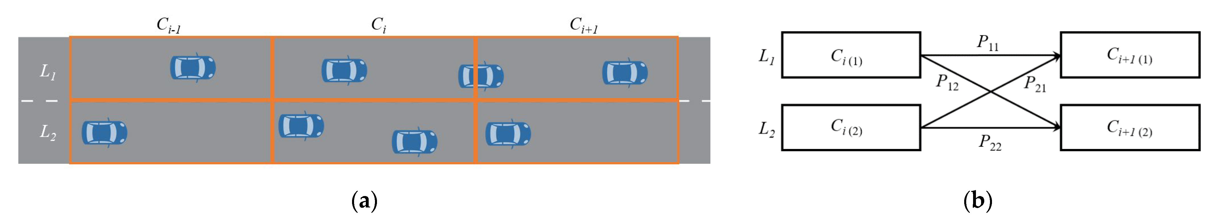
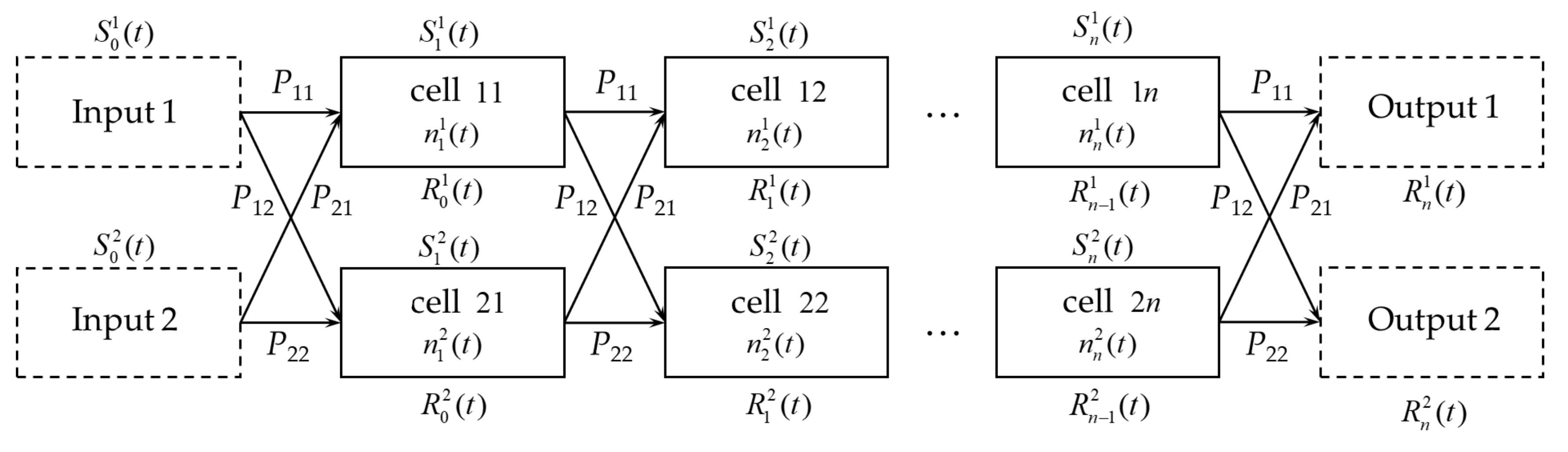
2.3. Double Lanes CTM

Daganzo established the CTM [34] with the concept of cellular automata to discretize time and space, which can describe the formation and dissipation of shock waves and queues and expand the scope of traffic flow mechanic properties from micro- to meso-level. Firstly, divide the time domain, making the research scope large enough to enable all vehicles to pass. Secondly, divide the road into sections according to fixed length, called cells. The cell length should be a distance that a vehicle normally travels in a free-flow state for a time step.

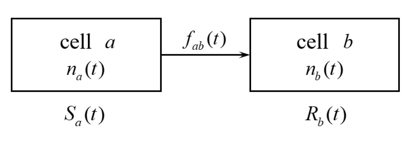
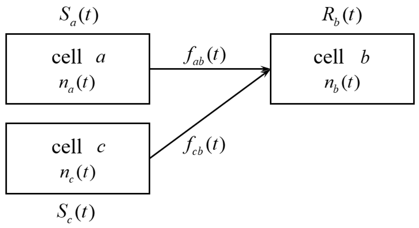
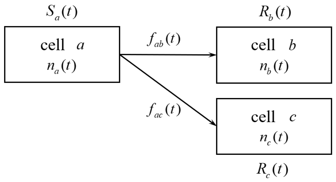
2.3.1. Cell Connection

There are three primary forms of cell connection; namely, direct connection, convergent connection, and divergent connection.

• Normal cell

As shown in Figure 3, for a simple connection between cells, the inbound traffic flow is equal to the outbound traffic flow at a node, and there is no convergence or divergence between cells. Cell $b$ is the downstream cell of cell $a$, $n_a(t)$ is the number of vehicles in cell $a$ on current step $t$, $n_b(t)$ is the number of vehicles in cell $b$ on the current step $t$, $S_a(t)$ is the supply of cell $a$ on the current step $t$, and $R_b(t)$ is the demand of cell $b$ on the current step $t$.

From the perspective of supply and demand, the actual traffic flow $f_{ab}(t)$ from cell $a$ to downstream cell $b$ on time step $t$ is expressed as follows:

$$f_{ab}(t)=\min \{S_a(t),R_b(t)\}$$

(15)

• Convergent cell

As shown in Figure 4, the flow of cell $a$ and cell $c$ converges into cell $b$. $n_c(t)$ is the number of vehicles in cell $c$ on the current step $t$, and $S_c(t)$ is the supply of cell $c$ on the current step $t$.

At this time, the actual traffic flow $f_{ab}(t)$ from cell $a$ to downstream cell $b$ on step $t$ and the existing traffic flow $f_{cb}(t)$ from cell $c$ to downstream cell $b$ on step $t$ are expressed as follows:

$$f_{ab}(t)=\left\{\begin{array}{l}{S}_a(t)\begin{array}{c}\begin{array}{c},\begin{array}{c}\end{array}{S}_a(t)+S_c(t)<R_b(t)\end{array}\end{array}\\ \min \{S_a(t),R_b(t)-S_c(t),(1-\alpha )R_b(t)\},\begin{array}{c}\end{array}else\end{array}\right.$$

(16)

$$f_{cb}(t)=\left\{\begin{array}{l}{S}_c(t)\begin{array}{c}\begin{array}{c},\begin{array}{c}\end{array}{S}_a(t)+S_c(t)<R_b(t)\end{array}\end{array}\\ \min \{S_c(t),R_b(t)-S_a(t),\alpha R_b(t)\},\begin{array}{c}\end{array}else\end{array}\right.$$

(17)

where $\alpha$ is the import rate, $0\le \alpha \le 1$.

• Divergent cell

As shown in Figure 5, the flow of cell $a$ diverges into cell $b$ and cell $c$.

Similarly, from the perspective of supply and demand, the actual traffic flow $f_{ab}(t)$ from cell $a$ to downstream cell $b$ on step $t$, and the actual traffic flow $f_{ac}(t)$ from cell $a$ to downstream cell $c$ on step $t$ are expressed as follows:

$$f_{ab}(t)=\min \{(1-\beta )S_a(t),R_b(t)\}$$

(18)

$$f_{ac}(t)=\min \{\beta S_a(t),R_c(t)\}$$

(19)

where, $\beta$ is divergence rate, $0\le \beta \le 1$.

2.3.2. Dynamic Cell Transfer

The mesoscopic cell transfer process of double lanes is designed as Figure 6 shows.

The flow transferring between cells on current step $t$ on the first lane $f_i^1(t)$, and on the second lane $f_i^2(t)$ are shown as follows, where $f_i^1(t),f_i^2(t),i\in [0,n]$.

$$\begin{array}{l}{f}_i^1(t)=\min \{S_i^1(t)\times P_{11}+S_i^2(t)\times P_{21},R_i^1(t)\}\\ f_i^2(t)=\min \{S_i^2(t)\times P_{22}+S_i^1(t)\times P_{12},R_i^2(t)\}\\ S_i^1(t)=\min \{Q_i^1,v_f^1{k}_i^1(t)\}\\ S_i^2(t)=\min \{Q_i^2,v_f^2{k}_i^2(t)\}\\ R_i^1(t)=\min \{Q_{i+1}^1,w^1(k_{jam}^1-k_{i+1}^1(t))\}\\ R_i^2(t)=\min \{Q_{i+1}^2,w^2(k_{jam}^2-k_{i+1}^2(t))\}\end{array}$$

(20)

Combining Equations (12), (13) and (20), double lanes CTM is obtained.

3. Simulation Experiment Results

The vehicle trajectory data of California I-80 highway in the Next Generation Simulation (NGSIM) data set of the United States is used for analysis, which is 1650 feet in length. To study the dynamic transfer process of traffic flow dominated by free lane-changing in double lanes, we selected lane 1 and lane 2 of I-80 highway, which were least impacted by forced lane-changing. We divided the searching area into a cell by 50 m, and record the number of vehicles, the number of vehicles with free lane-changing, average speed, and average density counted every 2 s in each cell of each lane. In addition, it is necessary to calculate the average speed difference and average density difference of cells between adjacent upstream and downstream cells in different lanes. Finally, normalize the data obtained, unifying variables of different dimensions.

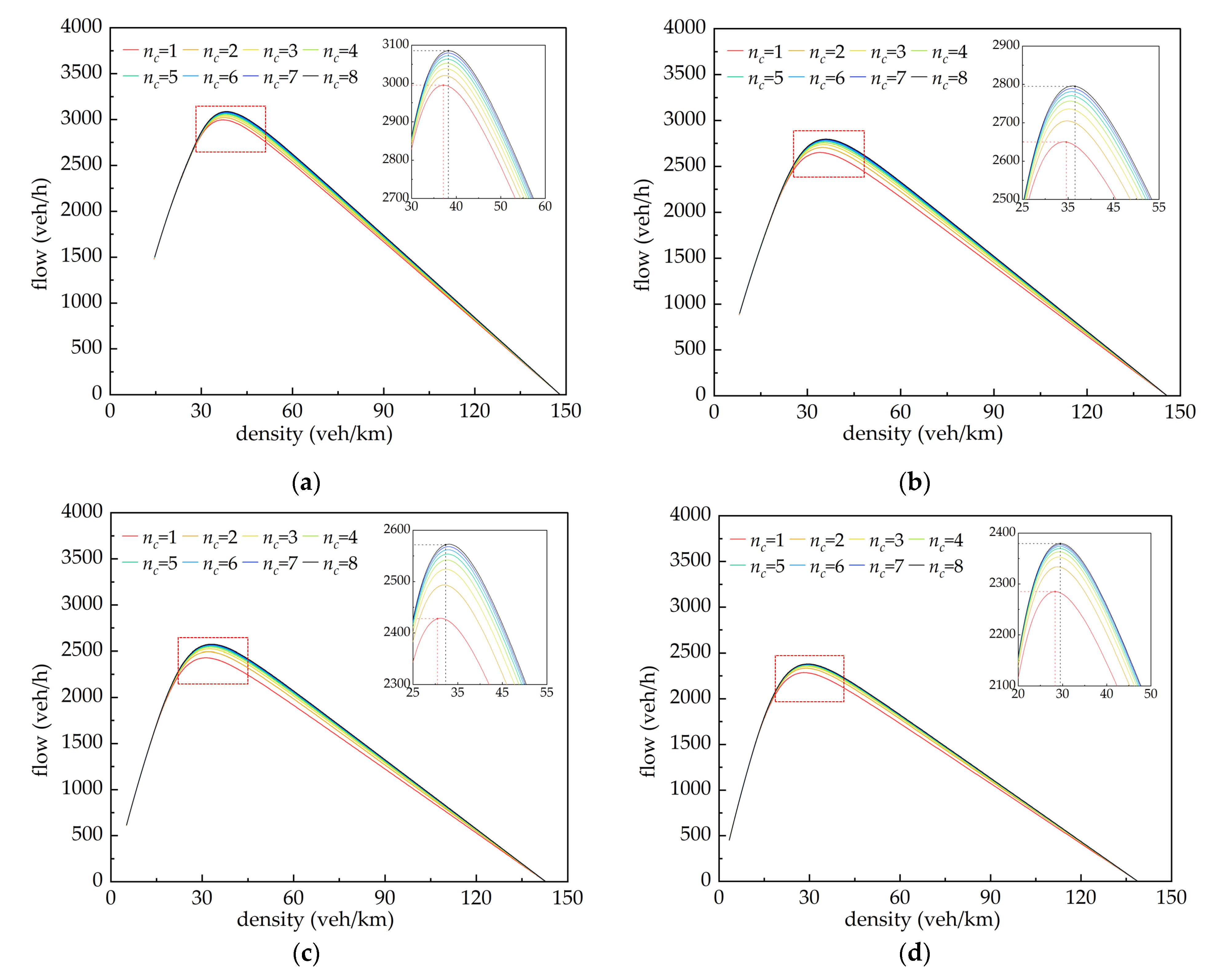
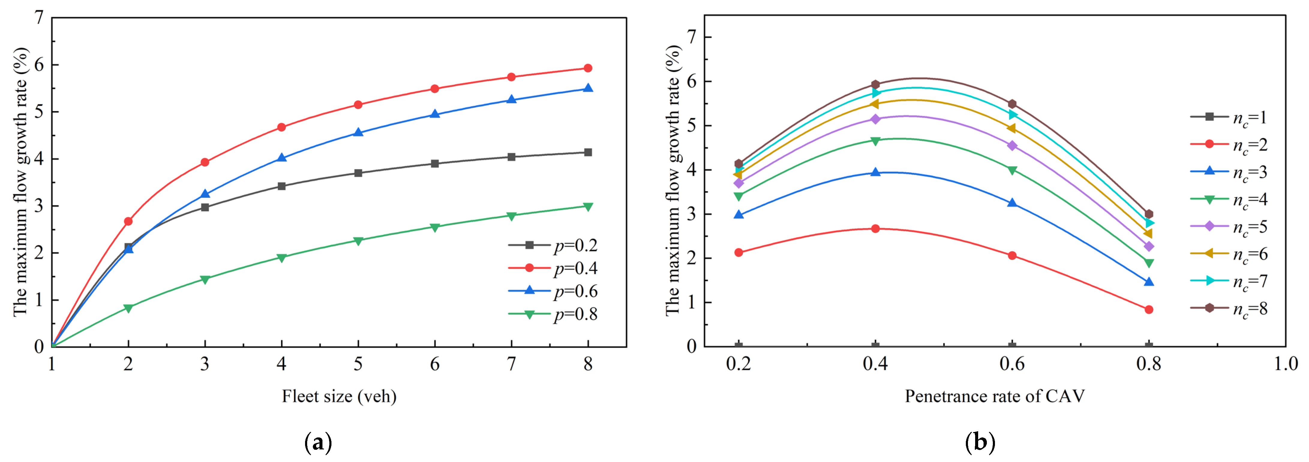
3.1. Mixed-Traffic Flow Fundamental Diagram Considering Fleet

According to Equation (7), the fundamental diagram of mixed-traffic flow with mixed motorcades can be obtained, which is primarily affected by the fleet size and CAV penetration rate. In Figure 7, the length of vehicle is $l=5 \mathrm{m}$, minimum safe distance is $\tilde{s}=2 \mathrm{m}$, free flow speed is $\tilde{v}=33.3 \mathrm{m}/s$, HV expected safe time headway is $T_h=1.5 \mathrm{s}$, AV expected safe time headway is $T_a=1.2 \mathrm{s}$, and CAV expected safe time headway is $T_c=0.6 \mathrm{s}$.

The maximum capacity of mixed-traffic flow gradually increases with the CAV penetrance rate. When fleet size $n_c=1$ and CAV penetrance rate $p=0.8$, the maximum flow increases by 710 veh/h when $p=0.2$. When fleet size $n_c=8$ and CAV penetrance rate $p=0.8$, the maximum flow increases by 706 veh/h when $p=0.2$. With the rise of CAV penetrance rate, critical density and congestion density grows, and road capacity is effectively improved. It is obtained from each diagram that CAV penetrance rate increases with the increase of fleet size; additionally, the maximum traffic capacity increases gradually as well as the critical density, while the congestion density remains the same. According to the fundamental diagram of mixed-traffic flow in Figure 7, the road capacity is analyzed with changes of CAV penetrance rate and fleet size, and intuitively exhibit the growth rate of maximum flow (based on fleet size $n_c=1$).

It can be seen in Figure 8a that when the CAV penetration rate $p=0.4$, the maximum flow growth rate always maintains a relatively high level; that is, the traffic capacity increases fastest. When $p=0.8$, the maximum flow growth rate tends to increase steadily. Therefore, it is believed that the capacity can only improve when the CAV penetration rate is within a certain range. In Figure 8b, when the fleet size $n_c\ge 6$, the maximum flow growth rate is more than $2.5\%$. Therefore, the capacity increases significantly when the fleet size is within $6-8$. In addition, the impact on traffic capacity caused by the continuous increase of fleet size is worth further exploring.

According to the analysis above, characteristic parameters of mixed-traffic flow with CAV penetration rate $p=0.4$ and $p=0.8$ of the fundamental diagram will be taken for comparison and analysis where there are only HVs.

Take traffic flow characteristic parameters when the CAV fleet $n_c=8$, penetrance rate $p=0.4$ and $p=0.8$ of the mixed-traffic flow fundamental diagram, and compare them with where there are only HVs running. The parameters are shown in

Table 1. Mixed-traffic flow characteristic parameters.

Parameter	Unit	CAV Penetration Rate
		$\mathit{p}=0$	$\mathit{p}=0.4$	$\mathit{p}=0.8$
$Q_i$	veh/h	2050	2572	3085
$v_f$	km/h	75.95	79.63	82.65
$w$	km/h	19.08	23.27	27.83
$k_{crit}$	veh/km	26.99	32.30	37.25
$k_{jam}$	veh/km	134.41	142.82	148.11

.

3.2. Utility Function Calibration

After processing, the sample size is balanced, and the data includes whether lane-changing is happening, the average speed and average density of current cells in different lanes, average speed difference, and average density difference between adjacent downstream cells.

We used SPSS to perform binomial logit regression on the processed data to obtain the final fitting result, which is shown in

Table 2. Variables in utility equation changing from lane 1 to lane 2.

	B	S.E.	Wals	df	Sig.
$\overline{k_1}$	3.895	0.563	47.880	1	0.000
$\overline{v_1}$	−4.287	0.544	62.062	1	0.000
$\Delta k_{12}$	−2.643	0.721	13.448	1	0.000
$\Delta v_{12}$	3.279	0.919	12.729	1	0.000
Constant	0.849	0.556	2.329	1	0.000

and

Table 3. Variables in utility equation changing from lane 2 to lane 1.

	B	S.E.	Wals	df	Sig.
$\overline{k_2}$	1.034	0.474	4.753	1	0.029
$\overline{v_2}$	−1.570	0.758	4.293	1	0.038
$\Delta k_{21}$	−2.752	0.686	16.102	1	0.000
$\Delta v_{21}$	3.436	0.924	13.842	1	0.000
Constant	−1.039	0.759	1.877	1	0.000

.

It can be found that the occurrence of free lane-changing between cells mainly depends on current traffic conditions of cells and benefits of adjacent downstream cells. The $p$ values of all parameters in each table are less than 0.05, indicating that these parameters have a significant impact on the utility function. Where lane-changing occurred is represented by 1, which is calculated in the output result, while where lane-changing did not occur is represented by 0. Therefore, the variable coefficients of utility function $V_{11}$ are the opposite of utility function $V_{12}$, the coefficients of utility function $V_{22}$ and utility function $V_{21}$ are the same.

The average density of the current cell has a positive relationship with the utility function, which means that the higher current cell density is, the easier it is to change lanes. The average speed of the current cell has a negative relationship with the utility function, means the lower current cell speed is, the easier it is to change lanes. The correlation of average density difference and average speed difference is also consistent with the actual situation. It can be seen from the classification table that prediction results are about 70% and 60%, as shown in

Table 4. Classification table in utility equation changing from lane 1 to lane 2.

		CL Has Been Predicted		Percentage Correction
		0	1
CL has been predicted	0	203	85	70.5
	1	91	197	68.4
Percentage in total				69.4

and

Table 5. Classification table in utility equation changing from lane 2 to lane 1.

		CL Has Been Predicted		Percentage Correction
		0	1
CL has been predicted	0	165	123	57.3
	1	107	181	62.8
Percentage in total				60.1

, considering the fitting results are acceptable.

Thus, the final utility function can be obtained:

$$V_{12}=3.895{\overline{k}}_1-4.287{\overline{v}}_1-2.643\Delta k_{12}+3.279\Delta v_{12}+0.849$$

(21)

$$V_{21}=1.034{\overline{k}}_2-1.570{\overline{v}}_2-2.752\Delta k_{21}+3.436\Delta v_{21}-1.039$$

(22)

This section may be divided using subheadings. It should provide a concise and precise description of the experimental results and their interpretation, as well as the experimental conclusions that can be drawn.

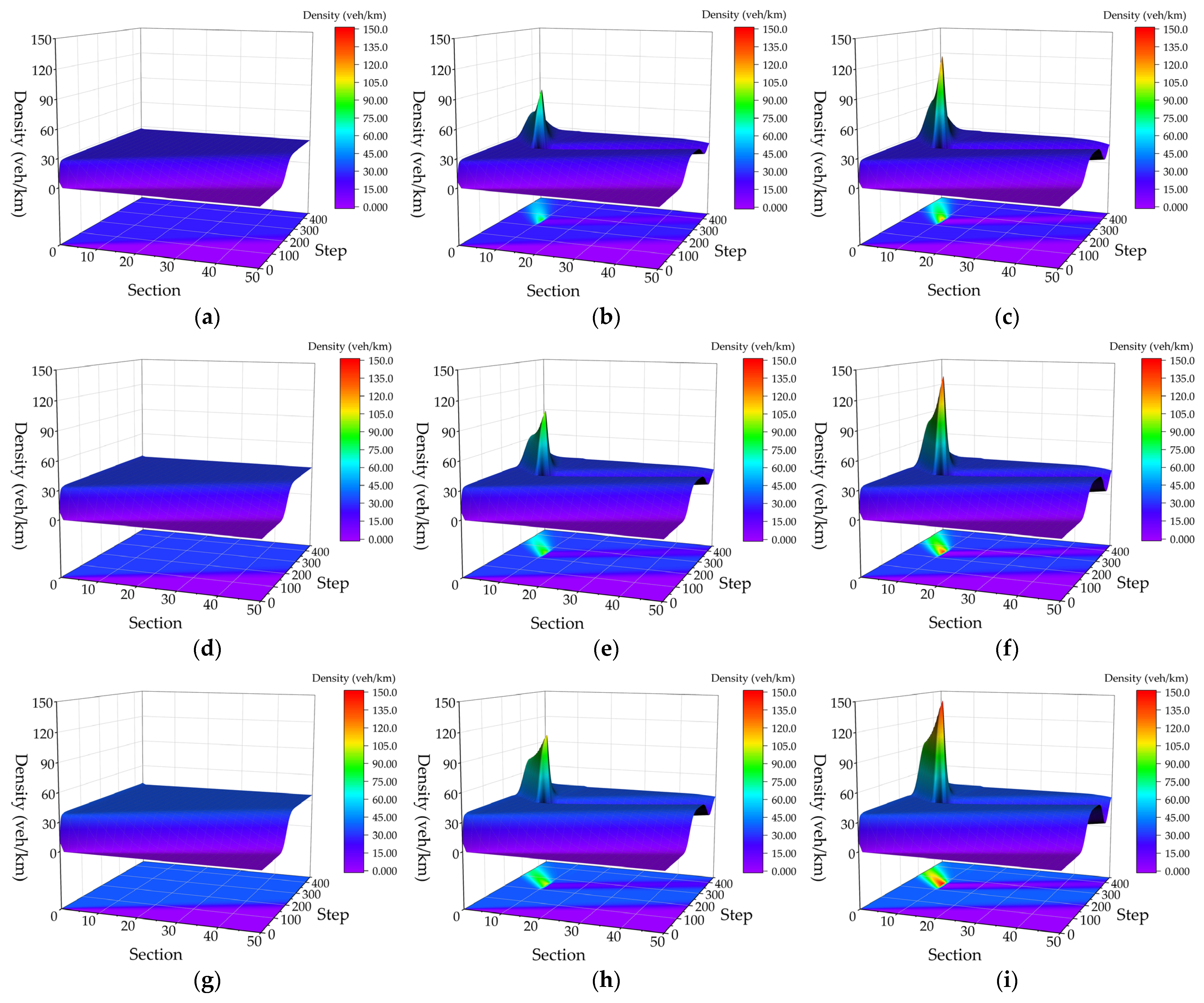
3.3. Dynamic Transmission Effect of Mixed-Traffic Flow

According to the above characteristic parameters of mixed-traffic flow obtained from the fundamental diagram, combined with the established double lanes CTM, shows the thermodynamic diagram of mixed-traffic flow in Figure 9.

With the increase in the CAV penetrance rate and fleet size, the average density of balanced-traffic flow raises for shorter average headway, as well as free-flow speed, transferring to downstream cells becomes faster. In the congestion state, when $L_2$ is closed, congestion occurs in $L_2$ immediately, in which case the lane changes to $L_1$, causing congestion. Upstream of the congested section, as the number of outbound vehicles has not decreased, the number of inbound vehicles is still increasing, congestion spreads forward. The congestion degree upstream of $L_1$ is less than that of $L_2$. Similarly, for the downstream section, leaving vehicles to run normally while the number of entering vehicles decreases, which improves downstream traffic conditions, and the downstream flow of $L_1$ is more stable than $L_2$. The increase of CAV penetration rate and fleet size improves free flow speed and congestion wave speed, leading to faster congestion occurrence and dissipation, which conforms to reality.

4. Conclusions and Discussion

This paper starts by analyzing the driving characteristics of HV, AV, and CAV, considering the distribution of vehicles and the fleet. The analytic expression considering CAV fleet in the equilibrium state is derived, constructing the fundamental diagram of mixed-traffic flow. A lane-changing judgment mechanism based on random utility theory was then developed. Double-lane CTM based on random utility theory was established, realizing dynamic transmission between lane-level cells. Compared with the research of Yu [35] on macro traffic flow, this paper retains the micro-characteristics of vehicles, refines the distribution of vehicles and the arrangement of fleets, and fully considers the influence of the fundamental diagram of mixed-traffic flow combined with vehicle driving characteristics on road capacity at the meso-level. Research of Pan [36] proposed the CTM taking the lane-changing motivation into account, which depends on the setting of multiple combined demand parameters with a specific priority. The lane-changing Judgment Mechanism established in this paper uses actual data to calibrate, and the calculation of lane-changing motivation considering driving revenue is less. The main conclusions are as follows:

(1)

With the increase of CAV penetrance rate $p$ and fleet size $n_c$, the capacity of mixed-traffic flow can be effectively improved, as well as the critical density and maximum flow.

(2)

When CAV penetration rate and fleet size are within a certain range, the capacity can be improved more clearly. When $p=0.4$, the maximum flow growth rate stays at a high level, and when fleet size $n_c$ is 6–8, the maximum flow growth rate is more than 2.5%.

(3)

Through analysis of simulation, it is verified that double lanes CTM established is in line with actual traffic flow change trend, proving effectiveness and feasibility of the model.

The model established in this paper reflects the influence of micro-car-following and lane-changing behavior at the meso-level and details the car-following characteristics of different types of vehicles and lane-changing rules. The random utility theory is applied to the judgment mechanism of free lane-changing, and dynamic double-lane flow transfer is realized by combining the traffic flow fundamental diagram model with CTM. Compared with previous studies, it thoroughly considered the influence of the fundamental diagram with vehicle-driving characteristics on the capacity at the mesoscopic level and developed the rules of lane-changing based on random utility theory in a mesoscopic view, which conforms to the inherent dynamic principle and operation mechanism of traffic flow. Since the mesoscopic traffic flow model only explores the mixed-traffic flow characteristics of double lanes, the characteristics of three lanes and above deserve further exploration and the application of multiple logit models. At the same time, the impact of intelligent vehicles on the road network can be deeply analyzed through the modeling of the urban traffic network and the study of traffic-flow transport mechanisms.

References

1. Shladover, S.E.; Su, D.; Lu, X.Y. Impacts of cooperative adaptive cruise control on freeway traffic flow. Transp. Res. Rec. 2012, 2324, 63–70. [Google Scholar] [CrossRef] [Green Version]
2. Milanes, V.; Shladover, S.E. Modeling cooperative and autonomous adaptive cruise control dynamic responses using experimental data. Transp. Res. Part C Emerg. Technol. 2014, 48, 285–300. [Google Scholar] [CrossRef] [Green Version]
3. Liu, H.; Kan, X.D.; Shladover, S.E.; Lu, X.Y.; Ferlis, R.E. Modeling impacts of cooperative adaptive cruise control on mixed traffic flow in multi-lane freeway facilities. Transp. Res. Part C Emerg. Technol. 2018, 95, 261–279. [Google Scholar] [CrossRef]
4. Lesch, V.; Breitbach, M.; Segata, M.; Becker, C.; Kounev, S.; Krupitzer, C. An overview on approaches for coordination of platoons. IEEE Trans. Intell. Transp. Syst. 2022, 23, 10049–10065. [Google Scholar] [CrossRef]
5. Guo, G.; Li, D. Adaptive sliding mode control of vehicular platoons with prescribed tracking performance. IEEE Trans. Veh. Technol. 2019, 68, 7511–7520. [Google Scholar] [CrossRef]
6. Gong, S.; Du, L. Cooperative platoon control for a mixed traffic flow including human drive vehicles and connected and autonomous vehicles. Transp. Res. Part B Methodol. 2018, 116, 25–61. [Google Scholar] [CrossRef]
7. Davis, L.C. Dynamics of a long platoon of cooperative adaptive cruise control vehicles. Phys. A 2018, 503, 818–834. [Google Scholar] [CrossRef]
8. Lee, W.J.; Kwag, S.I.; Ko, Y.D. The optimal eco-friendly platoon formation strategy for a heterogeneous fleet of vehicles. Transp. Res. Part D Transp. Environ. 2021, 90, 102664. [Google Scholar] [CrossRef]
9. Zhao, W.; Ngoduy, D.; Shepherd, S.; Liu, R.; Papageorgiou, M. A platoon based cooperative eco-driving model for mixed automated and human-driven vehicles at a signalised intersection. Transp. Res. Part C Emerg. Technol. 2018, 95, 802–821. [Google Scholar] [CrossRef] [Green Version]
10. Yao, Z.; Hu, R.; Wang, Y.; Jiang, Y.; Ran, B.; Chen, Y. Stability analysis and the fundamental diagram for mixed connected automated and human-driven vehicles. Phys. A 2019, 533, 121931. [Google Scholar] [CrossRef]
11. Yao, Z.; Gu, Q.; Jiang, Y.; Ran, B. Fundamental diagram and stability of mixed traffic flow considering platoon size and intensity of connected automated vehicles. Phys. A 2022, 604, 127857. [Google Scholar] [CrossRef]
12. Vranken, T.; Schreckenberg, M. Modelling multi-lane heterogeneous traffic flow with human-driven, automated, and communicating automated vehicles. Phys. A 2022, 589, 126629. [Google Scholar] [CrossRef]
13. Bando, M.; Hasebe, K.; Nakayama, A.; Shibata, A.; Sugiyama, Y. Dynamical model of traffic congestion and numerical simulation. Phys. Rev. E 1995, 51, 1035–1042. [Google Scholar] [CrossRef]
14. Helbing, D.; Tilch, B. Generalized force model of traffic dynamics. Phys. Rev. E 1998, 58, 133–138. [Google Scholar] [CrossRef] [Green Version]
15. Peng, G.; Lu, W.; He, H. Nonlinear analysis of a new car-following model accounting for the global average optimal velocity difference. Mod. Phys. Lett. B 2016, 30, 1650327. [Google Scholar] [CrossRef]
16. Li, X.; Qie, L.; Liu, Z.; Dong, Z.; Wei, S. Numerical simulation of car-following model considering multiple-velocity difference and changes with memory. In Proceedings of the 2021 2nd International Conference on Electronics, Communications and Information Technology (CECIT), Sanya, China, 27–29 December 2021; pp. 777–782. [Google Scholar]
17. Wang, E.; Yang, T. Car following behavior analysis of different types of vehicles on ten lane expressway based on cellular automata. In Proceedings of the 2021 6th International Conference on Transportation Information and Safety (ICTIS), Wuhan, China, 22–24 October 2021; pp. 1576–1581. [Google Scholar]
18. Gipps, P.G. A model for the structure of lane-changing decisions. Transp. Res. Part B Methodol. 1986, 20, 403–414. [Google Scholar] [CrossRef]
19. Yang, Q.; Koutsopoulos, H.N. A Microscopic Traffic Simulator for evaluation of dynamic traffic management systems. Transp. Res. Part C Emerg. Technol. 1996, 4, 113–129. [Google Scholar] [CrossRef]
20. Balal, E.; Cheu, R.L.; Sarkodie-Gyan, T. A binary decision model for discretionary lane changing move based on fuzzy inference system. Transp. Res. Part C Emerg. Technol. 2016, 67, 47–61. [Google Scholar] [CrossRef]
21. Peng, J.; Guo, Y.; Fu, R.; Yuan, W.; Wang, C. Multi-parameter prediction of drivers’ lane-changing behaviour with neural network model. Appl. Ergon. 2015, 50, 207–217. [Google Scholar] [CrossRef]
22. Dou, Y.; Yan, F.; Feng, D. Lane changing prediction at highway lane drops using support vector machine and artificial neural network classifiers. In Proceedings of the 2016 IEEE International Conference on Advanced Intelligent Mechatronics (AIM), Banff, AB, Canada, 12–15 July 2016; pp. 901–906. [Google Scholar]
23. Talebpour, A.; Mahmassani, H.S.; Hamdar, S.H. Modeling lane-changing behavior in a connected environment: A game theory approach. Transp. Res. Procedia 2015, 7, 420–440. [Google Scholar] [CrossRef] [Green Version]
24. Hoogendoorn, R.; van Arerm, B.; Hoogendoom, S. Automated driving, traffic flow efficiency, and human factors: Literature review. Transp. Res. Rec. 2014, 2422, 113–120. [Google Scholar] [CrossRef]
25. Ngoduy, D. Platoon-based macroscopic model for intelligent traffic flow. Transp. B Transp. Dyn. 2013, 1, 153–169. [Google Scholar] [CrossRef]
26. Delis, A.I.; Nikolos, I.K.; Papageorgiou, M. Macroscopic traffic flow modeling with adaptive cruise control: Development and numerical solution. Comput. Math. Appl. 2015, 70, 1921–1947. [Google Scholar] [CrossRef]
27. Levin, M.W.; Boyles, S.D. A multiclass cell transmission model for shared human and autonomous vehicle roads. Transp. Res. Part C Emerg. Technol. 2016, 62, 103–116. [Google Scholar] [CrossRef] [Green Version]
28. Tiaprasert, K.; Zhang, Y.; Aswakul, C. Closed-form multiclass cell transmission model enhanced with overtaking, lane-changing, and first-in first-out properties. Transp. Res. Part C Emerg. Technol. 2017, 85, 86–110. [Google Scholar] [CrossRef]
29. Nagalur Subraveti, H.H.; Knoop, V.L.; van Arem, B. First order multi-lane traffic flow model—An incentive based macroscopic model to represent lane change dynamics. Transp. B Transp. Dyn. 2019, 7, 1758–1779. [Google Scholar] [CrossRef] [Green Version]
30. Mahmassani, H.S. Autonomous vehicles and connected vehicle system: Flow and operations considerations. Transp. Sci. 2016, 50, 1140–1162. [Google Scholar] [CrossRef]
31. Zong, F.; Wang, M.; Tang, M.; Li, X.; Zeng, M. An improved intelligent driver model considering the information of multiple front and rear vehicles. IEEE Access 2021, 9, 66241–66252. [Google Scholar] [CrossRef]
32. Qin, Y.; Wang, H.; Wang, W.; Wan, Q. Fundamental diagram model of heterogeneous traffic flow mixed with CACC vehicles and ACC vehicles. China J. Highw. 2017, 30, 127–136. [Google Scholar]
33. Subirana, B.; Perez-Sanchis, M.; Sarma, S. Randomness in transportation utility models: The triangular distribution may be a better choice than the normal and gumbel. In Proceedings of the 2017 IEEE 20th International Conference on Intelligent Transportation Systems (ITSC), Yokohama, Japan, 16–19 October 2017; pp. 1–6. [Google Scholar]
34. Daganzo, C.F. The cell transmission model: A dynamic representation of highway traffic consistent with the hydrodynamic theory. Transp. Res. B Methodol. 1994, 28, 269–287. [Google Scholar] [CrossRef]
35. Yu, H.; Diagne, M.L.; Zhang, L.; Krstić, M. Bilateral boundary control of moving shockwave in LWR model of congested traffic. IEEE Trans. Automat. Contr. 2019, 66, 1429–1436. [Google Scholar] [CrossRef]
36. Pan, T.; Lam, W.H.K.; Sumalee, A.; Zhong, R. Multiclass multilane model for freeway traffic mixed with connected automated vehicles and regular human-piloted vehicles. Transp. A Transp. Sci. 2021, 17, 5–33. [Google Scholar] [CrossRef]
Figure 1. Structure of the paper.
Energies 16 03108 g001
Figure 3. Direct connection between cells.
Energies 16 03108 g003
Figure 4. Convergent connection among cells.
Energies 16 03108 g004
Figure 5. Divergent connection among cells.
Energies 16 03108 g005
Figure 6. Double lanes traffic flow dynamic transfer process.
Energies 16 03108 g006
Figure 7. Fundamental diagram of different CAV fleet size and penetrance rate with (a) p = 0.2 ; (b) p = 0.4 ; (c) p = 0.6 ; (d) p = 0.8 .
Energies 16 03108 g007
Figure 8. Change of maximum flow growth rate with (a) fleet size and (b) CAV penetrance rate.
Energies 16 03108 g008
Figure 9. There are all HVs on the road under (a) the free flow state; (b) the state of L 1 ; (c) the state of L 2 respectively showing the congestion expresses on different lands. When CAV penetration rate is 0.4 under (d) the free flow state; (e) the congestion state of L 1 ; (f) the congestion state of L 2 . Similarly, when CAV penetration rate is 0.8 under (g) the free flow state; (h) the congestion state of L 1 ; (i) the congestion state of L 2 .
Energies 16 03108 g009