Article

Performance Study on an Electrocaloric Heat Pump Based on Ga-Based Liquid Metal

1
School of Mechanical Engineering, Beijing Institute of Technology, Beijing 100081, China
2
State Key Laboratory of Automotive Safety and Energy, Tsinghua University, Beijing 100084, China
3
China North Vehicle Research Institute, Beijing 100072, China
*
Author to whom correspondence should be addressed.
Energies 2023, 16(7), 3104; https://doi.org/10.3390/en16073104
Submission received: 18 February 2023 / Revised: 14 March 2023 / Accepted: 27 March 2023 / Published: 29 March 2023
(This article belongs to the Special Issue Advances in Thermal Energy Storage and Applications)

Abstract

:
A solid-state heat pump using the electrocaloric effect (ECE) provides a new idea for the future development of heat pumps. However, most of the electrocaloric (EC) heat pumps presented in the literature are low in efficiency and use at least one moving part, which significantly reduces the reliability of the heat pump and adds to its complexities. In this context, combining the positive and negative ECEs, we proposed a plate-laminar non-mobile EC heat pump adopting Gallium-based liquid metal as an intermediate medium to guarantee highly efficient heat transfer. Numerical simulation in COMSOL Multiphysics has been performed to investigate the correlation between different operating parameters and the performance of the EC heat pump. Changing the temperature span only, a COP of 8.13 and a UVHP of 746.1 W · d m 3 were obtained at a temperature span of 7 K. It was also found that the UVHP increased by 28.45% and COP increased by 25.46% after adding one layer of EC material. The electric-induced quantity of heat and cooling capacity was found to significantly affect the heating performance. The biggest heating power of 7132.7 W · d m 3 was obtained under 200 M V · m 1 , and the biggest COP of 14.84 was obtained under 150 M V · m 1 at a cyclic period of 8 s. This study provides a highly efficient, non-mobile EC heat pump that employs fluid-thermal conjugated heat transfer, and exploration of the parameters makes the optimization of the heat pump possible by fine-tuning the operation parameters.

1. Introduction

As a kind of renewable energy equipment driven by electricity, heat pumps obtain waste heat and other low-grade energy from environmental mediums to provide available high-grade heat energy. It can yield three times or more heat per portion of the energy consumed, which has greatly improved energy utilization efficiency, and it is also an efficient and energy-saving energy product [1]. The steam compression system is the main application form of the heat pump, but it is complex in structure, large in volume, low in efficiency, and traditional artificial refrigerants such as freon are the main factors leading to global warming. As the Montreal Protocol and its amendments come into effect, countries have tightened controls on refrigerants with strong greenhouse effects [2].
EC refrigeration technology has recently developed and become a research hotspot because of the advent of new EC materials. The energy reversibility of EC materials is high (>90%), and the energy of the actuating electric field can be efficiently recovered and reused (>80%). Other advantages of the EC materials include the simple way to impose the electric field, the light equipment, and the simple system structure [
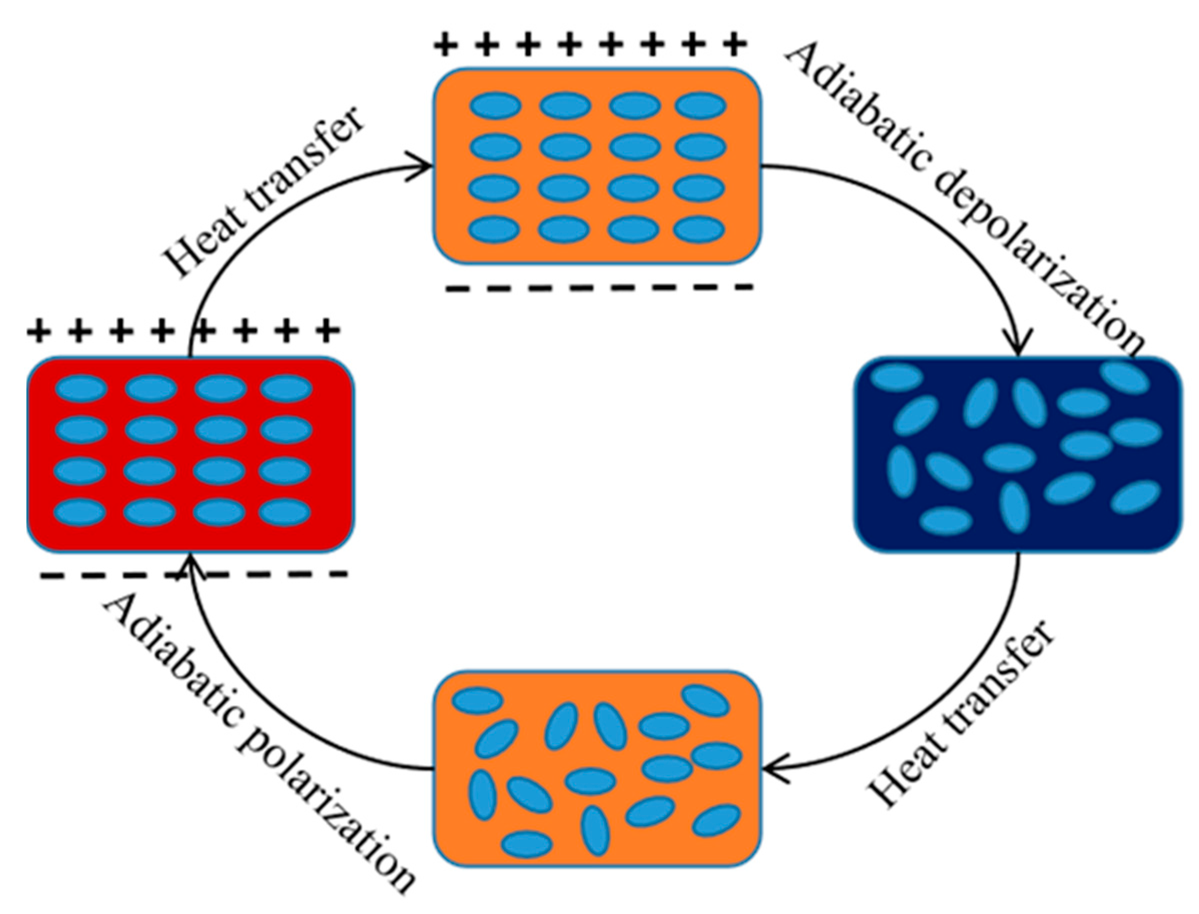
3]. Hence, EC refrigeration or heat pump technology is well known as a promising solid-state refrigeration or heat pump technology. ECE refers to the temperature or entropy change caused by the external electric field in polar materials. An adiabatic temperature change greater than 10 K in EC materials is generally known as the “giant ECE” [4]. Initially, because the ECE in the EC material and its adiabatic temperature change were too small, the development of EC refrigeration technology was seriously limited. It was not until the 21st century that there was some progress in EC materials. Professor Zhang Qiming [5] discovered the giant ECE in ceramic and polymer materials in 2006. Subsequently, Neese [6] found the giant ECE in ferroelectric polymer P(VDF-TrFE-CFE) near room temperature, which laid the foundation for the application of the ECE in the actual refrigeration or heat pump device and thus contributed to the emergence of a series of EC models and devices. Although the ECE has been studied for nearly 20 years, the developed models and numerical investigations proposed in the literature still need to grow. EC devices are divided into different types according to whether there are intermediate heat-carrying mediums and whether the EC module can be moved. The first EC devices have no moving parts or intermediate heat-carrying mediums. Farrukh Najmi [7] first proposed a conceptual prototype of an all-solid heat pump using two layers of EC material without moving parts, and the heat was transferred during three steps theoretically. Since there is no auxiliary heat transfer fluid, the heat exchange of the heat pump completely depends on the EC material itself. Guo et al. [8] proposed the first three-dimensional fluid-based EC refrigeration device, categorized as an intermediate heat-carrying fluid refrigeration device without moving parts. Brahim K et al. [9] also designed an EC device based on different nanofluids. In such immovable EC devices, heat transfer efficiency can be improved effectively by introducing an intermediate heat-carrying medium. The COP reached around 10, and a temperature span of more than 10 degrees was obtained.
The third kind of EC device has moving parts but no intermediate medium. Haiming Gu et al. [10] manufactured and studied an EC oscillatory refrigeration device (ECOR) for chip-level refrigeration, in which the EC module moved from the left side to the right side periodically to transport the heat and establish the temperature gradient within both the EC module and regenerator. Nevertheless, experimental and simulation results showed that the temperature span achieved by the device is no more than 3 K. Moreover, a similar movable EC device was designed by Ma et al. [11]. Laminate sheets of EC material that could be moved up and down were confined between the heat source and heat sink. Then, Yuan Meng et al. [12] designed a cascade EC cooling device with a similar structure in 2020, and the maximum temperature lift (no thermal load) was 8.7 K. These devices cannot obtain a large temperature span because the high thermal interface resistance exists among different pieces of EC solid materials, resulting in low heat transfer efficiency in the EC device. The last kind of EC device has moving parts and intermediate heat-carrying mediums. Yanbing Jia and Y. Sungtaek Ju reported a continuous EC refrigeration cycle with glycerol as a thermal interface to achieve reliable high-contrast thermal switching between an EC material and a heat source/sink [13]. However, due to the limitation of EC materials, the maximum temperature span achieved by the device could only reach about 1 Kelvin, and the mechanical drive increased the instability of the device. Qiang Li et al. designed an efficient rotating ECOR device based on the relaxation ferroelectric polymer P(VDF-TrFE-CFE). The EC parts rotate periodically through the electric field region, and the fluid flows through the EC parts to transfer the heat [14,15]. With the introduction of ferroelectric polymers having the giant ECE, the cooling performance of the device was improved to some extent with COP no more than 8 and a temperature span no more than 10 K. However, the rotating structure greatly increases the complexity and unreliability of the device, making it difficult to conduct experiments practically.
In brief, using a proper intermediate heat-carrying medium would improve heat transfer efficiency, and the immovability of the device would significantly increase the device’s reliability and reduce the device’s complexity, making it easy to apply. Most above-mentioned EC devices are removable, which greatly increases the complexity of the devices, and they have some disadvantages like low temperature spans, small COP, and small power density. Therefore, there is still much space for future progress in the research of highly efficient EC refrigeration or heat pump devices. In particular, EC material with giant ECE and heat transfer intensification are key to achieving the above goal. The former determines the upper limit of the temperature span that the EC device could achieve, which is mainly up to the material’s breakdown electric field strength. The latter may include a suitable configuration of heat transfer mediums, a reasonable structural design, and other factors so that the quantity of the heat and cooling capacity produced by the ECE could be utilized efficiently.
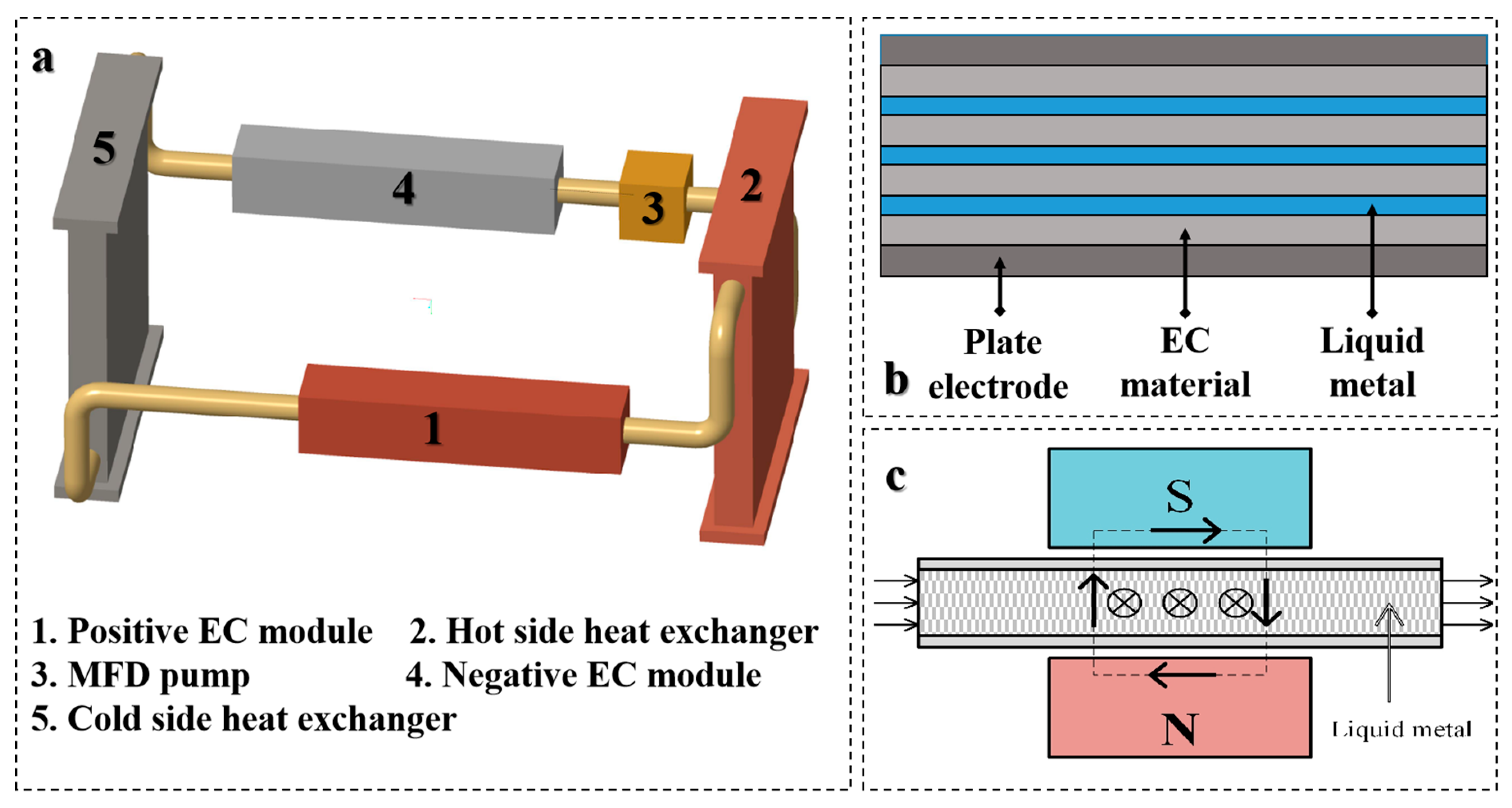
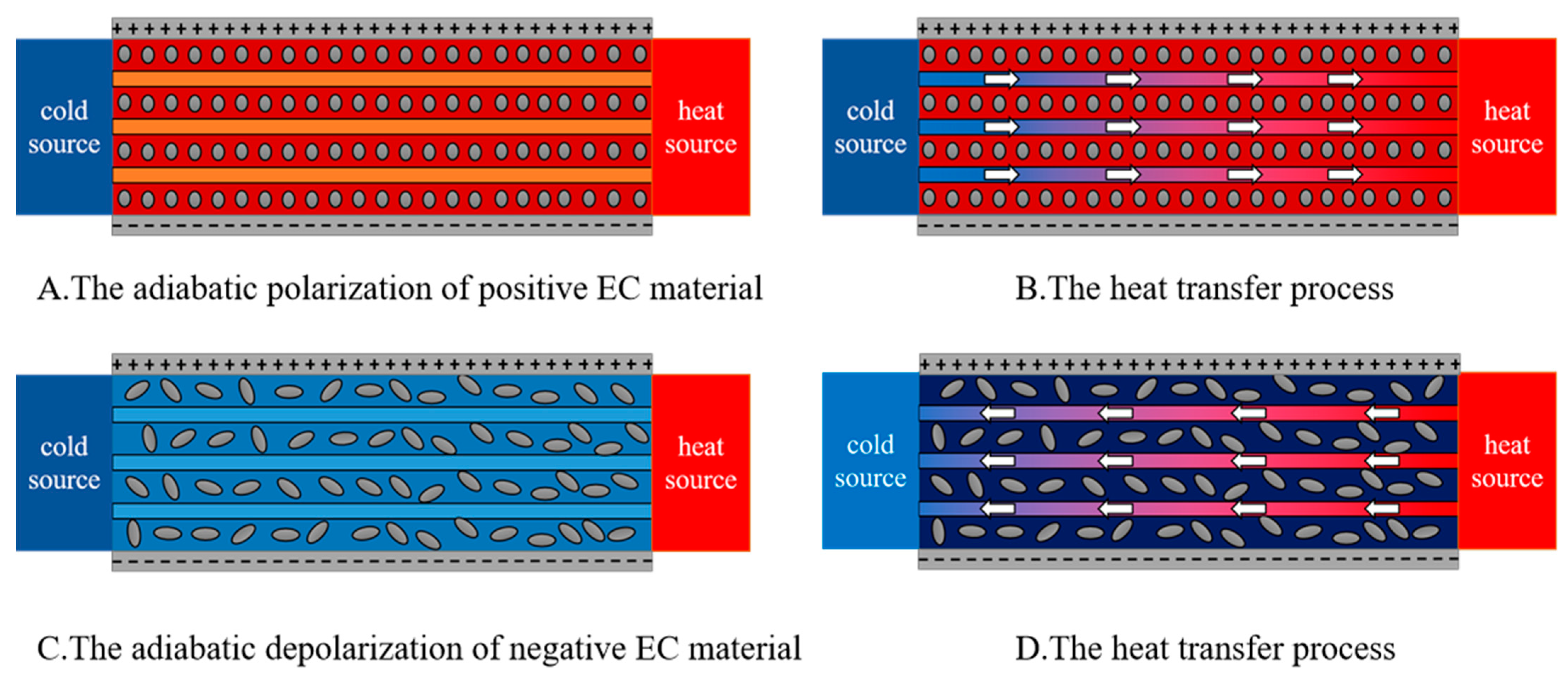
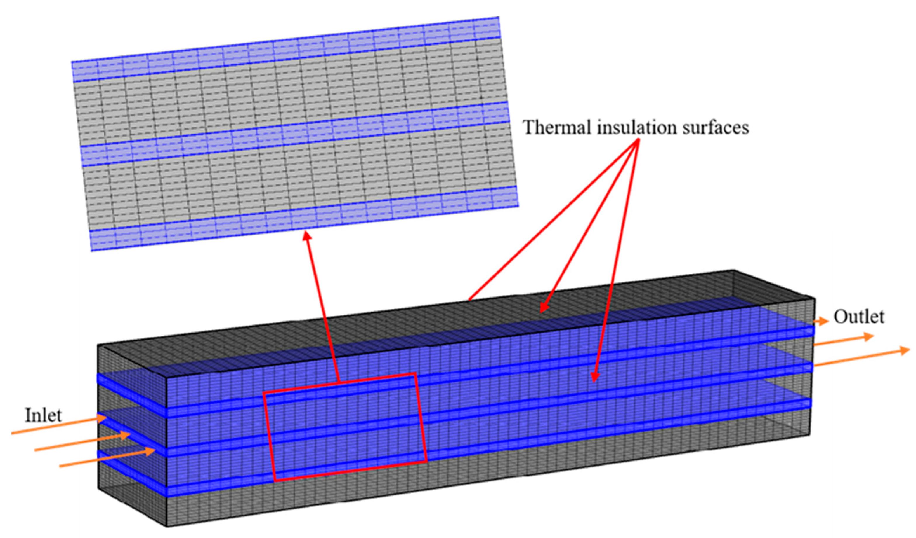
To design an EC heat pump with excellent performance, we innovatively use Ga-based liquid metal, which has super high thermal conductivity, as the heat transfer medium to effectively transfer the quantity of heat and cooling capacity produced by the EC material to the corresponding heat exchanger. Both positive ECE and negative ECE are utilized in a single cycle, and a simple layered structure is adopted to make the device easy to apply. Thus, a plate-laminar and non-mobile EC heat pump that uses Gallium-based liquid metal as the intermediate medium is designed, providing the possibility of substantial performance improvements and making it possible to apply the EC heat pump in an actual application scenario. The fluid–thermal conjugated (non-isothermal flow) heat transfer was employed to meet the demand for highly efficient and compact heat transfer. The positive and negative EC materials with giant ECE were made into thin films and stacked on top of each other to form a layered structure with channels in between where Gallium-based liquid metal flows to achieve highly efficient heat transfer. Compared with steam compression refrigeration, the positive EC material realized the function of the compressor, and the negative EC material acts as the expander. The performance of the EC heat pump was studied under different design and structural parameters. The study aims to find the relationship between different operational parameters and the performance of the EC heat pump to give reasonable optimization strategies and provide important guidance for the subsequent study of EC heat pumps.

2. Conceptual Design of the System

2.1. The Thermodynamic Principle of ECE

The ECE discovered by P. Kobeko [16] in 1930 in Rochelle is a physical phenomenon. The basic principle of the ECE is to load and unload the electric field to excite temperature change. As exhibited in Figure 1, when the electric field is applied to the EC material, the electric dipoles in the EC material will orientate from high degrees of freedom to low degrees of freedom. The entropy of the EC material drops, while the temperature increases if the process is considered adiabatic. After exchanging heat with the surroundings, the EC material reaches a state of thermal equilibrium. The electric field is then adiabatically removed from the EC material, and an adiabatic depolarization process occurs so that the EC material’s entropy increases and the temperature drops. Next, the EC material exchanges heat with surroundings again and returns to its original state. Meanwhile, for negative EC material, the principle is just the opposite. The temperature of the EC material decreases when the electric field is applied and increases when the electric field is removed. Supposing that the electric field is periodically applied to and removed from the EC material, the heat production and refrigerating capacity of the EC material can be utilized to obtain a complete thermodynamic cycle. Additionally, intermediate heat-carrying mediums can be used to improve heat transfer efficiency.

2.2. EC Heat Pump System Design

The EC heat pump designed in this paper is a non-mobile, plate-laminar EC structure which has three layers of fluid and four layers of EC material. This configuration indicates the best performance in terms of heat transfer efficiency. The non-mobile EC heat pump system shown in Figure 2a is composed by a positive EC module, a negative EC module, a magnetofluidodynamic pump (MFD pump), a hot heat exchanger, a cold heat exchanger, and pipes. Ga-based liquid metal circulates through the system to transfer a quantity of heat and cooling capacity. Figure 2c exhibits the detailed structure of the EC heat pump. The length and width of the EC heat pump are 25 mm and 5 mm, respectively, and the heights of the channels and the EC material are 0.3 mm and 1 mm, respectively. The total volume of the EC heat pump is 0.6125 cm3. The MFD pump utilizes amperage force generated by the coupling of electromagnetic fields to drive the liquid metal flow in the channel, and its detailed structure is shown in Figure 2c. Firstly, the electric field is applied on the positive EC module “1”. After its temperature rises, the MFD pump will drive the fluid from the cold side heat exchanger “5” through “1” into the hot side heat exchanger “2”. After reaching thermal equilibrium with the heat exchanger “2”, the electric field is then applied on the negative EC module “4”. The fluid continues to flow forward and transfer heat with the negative EC module “4” so that the fluid’s temperature decreases. Next, the fluid flows into the cold side heat exchanger. It then undergoes a period of heat transfer with the cold side heat exchanger and reaches thermal equilibrium again. The whole process requires a continuous input of electrical energy. By circling these cycles, the system can provide heating capacity continuously. Significantly, since the cyclic period is set before operation of the system, the fluid’s temperature at the end of the last cycle affects the next cycle.

2.3. EC Heat Pump’s Circulation Mechanism

The commonly used cycles of the EC heat pump are the Kano cycle, Eriksson cycle, Stirling cycle, and Breton cycle. Though the Kano cycle is ideal, it requires the cycle to run at four different electric field intensities. Moreover, the adiabatic temperature change of the EC material during iso-entropy polarization and depolarization limits the temperature difference between the cold and hot surroundings. The Eriksson cycle is irreversible, so its efficiency is low and cannot reach the ideal heat regeneration. The Stirling cycle is a regenerative cycle remarkably similar to the Ericsson one, but with the difference of being characterized by two isothermal and two iso-polarization processes instead of the two Ericsson’s iso-field processes. Although the Breton cycle cannot reach the efficiency of the Carnot one, it can exhibit optimal performances [17]. In this study, an EC heat pump is designed using the Breton cycle to enable heat regeneration. Combining Figure 2 and Figure 3, the detailed process of a cycle is as follows:
(a)
The adiabatic polarization of the positive EC module. The electric field is applied to the positive EC block (the EC block marked red in Figure 1), and the EC block’s temperature increases due to the positive ECE.
(b)
The heat transfer process. The electric field intensity is maintained at the maximum value, and the fluid flows through the channels between the EC layers to absorb heat from the EC material so that its own temperature increases. Next, the fluid flows into the hot heat exchanger to achieve heat accumulation.
(c)
The adiabatic polarization of negative EC module. The electric field is applied to the negative EC block (the EC block marked grey in Figure 1). The EC module’s temperature decreases due to the negative ECE.
(d)
The heat transfer process. The electric field intensity is maintained at the maximum value, and fluid flows through the channels to exchange heat with the EC material so that its own temperature drops, and then it flows into the cold heat exchanger to absorb heat from the surroundings.

2.4. EC Materials and Working Fluid

The magnitude of ECE is closely related to the electric field. Generally, EC materials can be divided into three categories, namely, monocrystals (bulk samples), ceramics (bulk samples, thick film ceramics and thin film ceramics), and polymers (thick and thin films) [12]. Thin and thick films can withstand at least two or three orders larger than bulk samples and monocrystals due to their much larger dielectric strength [18].
The ECE of positive EC material can be described by thermodynamic theory. It is worth noting that formulas (Equations (1)–(9)) are derived on the basis of reversible adiabatic processes of simple compressible materials. According to the law of energy conservation and the Maxwell relationship, entropy is the status parameter of simple compressible matter, which cannot be directly measured but is related to the basic status parameters (P, T, V) that can be directly measured. The Gibbs free energy [19] of the EC material is
G = U T S X i x i E i D i
U is the material’s internal energy, T is the temperature, S is the entropy, X is the stress, x is the strain, E is the electric field intensity, and D is the electric displacement vector. The differential form of the Formula (1) is
d G = S d T X i d x i D i d E i
Then, S, x i , and D i can be expressed as
S = ( G T ) X , E
x i = ( G X i ) T , E
D i = ( G E i ) T , X
Using Maxwell relations:
( S E i ) T , X = ( D i T ) X , E
The following equation is obtained:
( S E i ) T , X = ( D i T ) X , E = p
where p is the pyroelectric coefficient of the material.
Further, the adiabatic temperature change and isothermal entropy change of the material are obtained:
Δ T = T ρ E 1 E 2 1 C E ( D T ) E d E
Δ S = 1 ρ E 1 E 2 ( D T ) E d E
among which ρ and C E are the density and the heat capacity of the material at a constant electric field intensity. From Equations (8) and (9), it is known that a larger pyroelectric coefficient and a higher breakdown electric field intensity mean larger isothermal entropy change and adiabatic temperature change. Nevertheless, lower specific heat and density mean larger adiabatic temperature change when the isothermal entropy change remains constant. Ferroelectric materials have the largest pyroelectric coefficient at the paraelectric–ferroelectric phase transition temperature so that they have the greatest giant ECE compared with other dielectric materials [20].
Since ferroelectric materials have the biggest electrocaloric effect, ferroelectric polymer P(VDF-TrFE-CFE) was fabricated into laminar sheets and stacked on top of each other to form the EC module. Its physical properties are shown in Table 1. The application and removal of the electric field will result in hysteresis loss, but the hysteresis loss can be limited to below 5% in the ferroelectric polymer P (VDF-TrFE-CFE). Furthermore, its breakdown electric field intensity is 400 M V · m 1 , while the maximum setting electric field intensity is 200 M V · m 1 to avoid the possibility of the breakdown of the EC material.
In this work, an intermediate heat-carrying medium is set to flow through the channels formed by stacks of EC material, and it shall be capable of transferring heat with the EC material within a limited time and then exchanging heat with the corresponding heat exchanger. An intermediate medium with a small specific heat capacity and high thermal conductivity is required in this process.
Liquid metals with fluidic and metallic properties have low melting points near or below room temperature and therefore present a liquid state at around room temperature. Pure Gallium has a melting point of 29.6 °C, and a lower melting point is obtained when Gallium forms alloys with certain metals. The most notable of Gallium-based liquid metals are those formed by Gallium with elements such as In and Sn, whose melting points are generally around 10 °C, making them easy to apply at room temperature [21]. Moreover, they have attracted great attention owing to their special properties, including a low melting point (<30 °C), low toxicity, superior fluidity, high electronic conductivity, and excellent thermal conduction ability [22]. What is more, Gallium-based liquid metal is easy to obtain without a complicated preparation process. Due to these advantages, Gallium-based liquid metal has been largely applied in energy storage and conversion, catalysis, thermal management, biomedical healthcare, flexible electronics, soft robots [23], etc. Considering that the thermal conductivity of the liquid metal is relatively high, we applied it to the EC heat pump to achieve a larger range of temperature span. The liquid metal G a 61 I n 25 S n 13 Z n 1 with a melting point of 8 °C was used as the intermediate heat-carrying fluid to achieve highly efficient heat transfer. Water and nanofluid ( A l 2 O 3 ) simulations as intermediate heat-carrying fluids were also performed for comparison. Table 2 compares the characteristics of Gallium-based liquid metal, water, and nanofluid ( A l 2 O 3 ).

3. Model Settings

As shown in Figure 4, a flow chart was made to clearly show the research process of this paper.

3.1. Physical Model and Governing Equations

The numerical model is a three-dimensional model implemented in COMSOL Multiphysics as illustrated in Figure 5. Due to the limitation of COMSOL Multiphysics, we convert the positive and negative EC materials into one positive EC material in COMSOL Multiphysics, and the temperature increase and decrease of the EC material are achieved by periodically changing the electric field intensity. Non-isothermal flow occurs in the runners between the EC material. Since there is only one fixed inlet for the fluid during simulation, the upstream temperature of the inflow needs to be changed every half cycle. The simulation is carried out under the following assumptions: applying/removing the electric field is regarded as adiabatic; the physical properties of EC material and fluids are considered constant within the operating temperature range; the contact surface of the fluid and EC material has no thermal resistance; the temperatures of the hot heat exchanger and cold heat exchanger are constant; the initial temperature of the device is 25 °C.
This paper’s governing equation for the mathematical model of the EC heat pump consists of a series of coupled partial differential equations. The flow is described by the Navi-Stokes equation. The energy equation solves the temperature of the fluid and the solid domain:
ρ c p T t + ρ c p u · Δ T + · ( k T ) = Q ˙ E
The solution idea is as follows:
As is known from the Equation (10), to find out T, the required input parameters are the following:
(a)
Material properties (density, heat capacity at constant pressure, thermal conductivity).
(b)
Speed field u.
(c)
Heat source term. Formulas (8) and (9) reveal the internal mechanism of EC materials’ heat and entropy change, but these formulas cannot be directly written into COMSOL Multiphysics. Thanks to the work of Lu, SG and Rozic, B et al. [25], the heat source term Q ˙ E can be expressed as Formula 11, and it has been written into COMSOL Multiphysics to integrate the ECE and is defined as follows:
Q E · = ρ E T E ( S E E ) T E E T
among which E is the electric field intensity applied to the EC material, T E is the temperature of the EC material, S E is the entropy of the EC material, and ρ E is the density of the EC material. For the P(VDF-TrFE-CFE) terpolymer, the relationship between the entropy change and the electric field is as follows:
S E = C 1 E 2 + C 2 E
among which,
C 1 = 2.71 × 10 15   J · m 2 · k g 1 · K 1 · V 2 C 2 = 6.85 × 10 8   J · m · k g 1 · K 1 · V 1
Although the relationship between the entropy change and the electric field intensity is usually temperature-dependent, the ECE of this terpolymer does not change greatly in the temperature range of 270–320 K. For simplicity, the entropy change is assumed to be temperature-independent in this temperature range. In addition, the dielectric loss of this terpolymer is very small and could be ignored during simulation.

3.2. Boundary Conditions and Grid Settings

In our work, the fluid–thermal coupling model is used in COMSOL Multiphysics. The fluid domain is laminar flow, and the velocity that affects the temperature field is calculated using the Navi-Stokes equation. The fluid inlet and outlet boundary are set as the heat absorption surface and the heat rejection surface, respectively, as shown in Figure 5. To make the heat transfer process adiabatic, the surfaces indicated by the arrows in Figure 5 are set to be thermally insulated where the control equation is as follows:
n · q = 0
Additionally, a no-slip boundary condition is applied to the contact interface between the fluid and the solid. Since the geometry is a regular cuboid, the mapping and omitting method is used to create structured mesh for both the EC module and the fluid module successively. The verification of grid independence was carried out to make sure that the simulation results were insensitive to the grid number. As is exhibited in Figure 6, the variation of the volumetric average temperature of EC materials with time is no longer affected by the number of grids after the grid number exceeds 64,821. Furthermore, the verification of the numerical model in COMSOL Multiphysics was realized by comparing the temperature evolution of the corresponding EC device between Brahim’s work [9] and this work. As exhibited in Figure 7, the profiles are basically similar except for a few details which may be due to the differences in the electric field intensity and respective cyclic period.

4. Results and Discussion

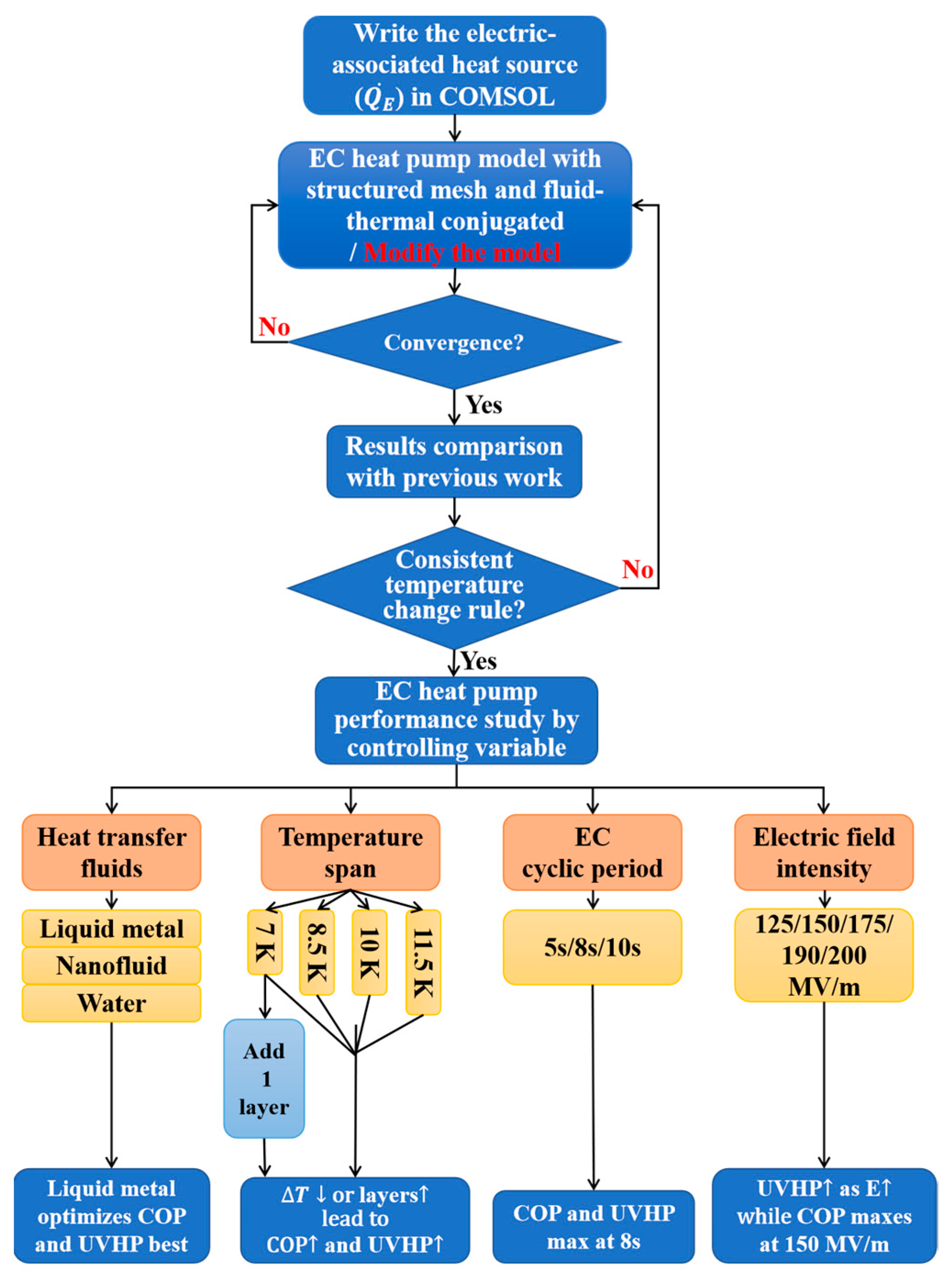
The simulations were carried out using the control variable method under different operating conditions. Coefficient of performance (COP) and unit volume heating power (UVHP) were used to evaluate the heating performance of the EC heat pump. COP measures the overall heating performance of the EC heat pump, while UVHP is an economic indicator. COP was defined as the ratio of the heating capacity to the electric power P consumed by the heat pump. As assumed, not only was there no heat leakage during the heat transfer process, but the energy loss of adiabatic temperature change of EC module was also not considered. Hence, according to the law of energy conservation, the consumed power is represented as
P = Q h Q c
Thus, the COP can be calculated as follows:
C O P = Q h Q h Q c
In addition, UVHP is defined as
U V H P = Q h V · Δ t = m f · c f · ( T h e a t T h ) V · Δ t = ρ f · u f · A · c f · ( T h e a t T h ) V
Subscript f indicates the fluid, subscript h indicates the hot heat exchanger, and subscript heat indicates the hot fluid after absorbing heat from the EC material.

4.1. Heating Performance of Different Heat Transfer Fluids

Using different heat transfer fluids for the same EC heat pump with the same boundary conditions and initial value will obtain different heat transfer effects. 
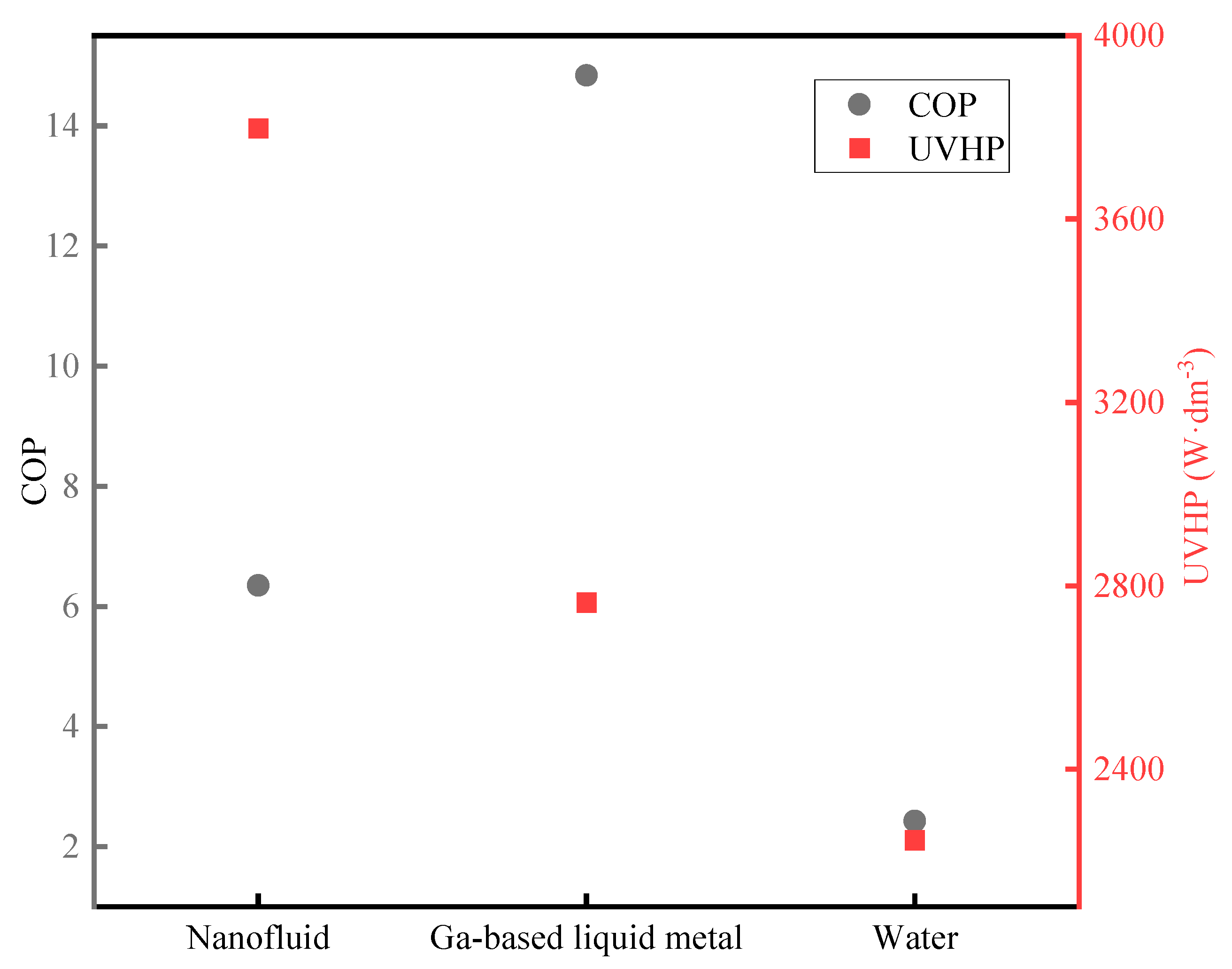
Figure 8 exhibits the COP and UVHP of the EC heat pump using different fluids as intermediate heat-carrying mediums at the temperature span of 10 K.
Water, as the intermediate heat-carrying fluid among the three fluids, has the smallest COP and UVHP. The COP of the EC heat pump using Gallium-based liquid metal as the intermediate heat-carrying medium is 2.34 times that of nanofluid and 6.12 times that of water. While the UVHP of the EC heat pump using nanofluid as the intermediate heat-carrying medium is 1.37 times that of Gallium-based liquid metal and 1.69 times that of water. COP measures the heat transfer efficiency of the EC heat pump, and UVHP is an economic indicator which reflects the unit volume heating capacity of the EC heat pump. Hence, the effect of liquid metal on heat transfer efficiency is greater than the effect of nanofluid on cost reduction. In addition, the economic consideration of this paper mainly refers to the EC material cost and intermediate heat-carrying fluid cost. Since there is only one EC device for different fluids, the EC material cost is the same. And it should be known that the preparation of nanofluid is more complicated than Gallium-based liquid metal, and there is the problem of particle aggregation. Thus, the actual heat transfer of nanofluid is greatly compromised compared to the simulation results. Because the fluid velocity was given determinately, greater density leads to greater mass flow, which is one of the reasons why the heat pump that uses nanofluid as the intermediate heat-carrying fluid has higher UVHP than that of the Gallium-based liquid metal. Therefore, Gallium-based liquid metal is the most suitable intermediate heat-carrying medium.

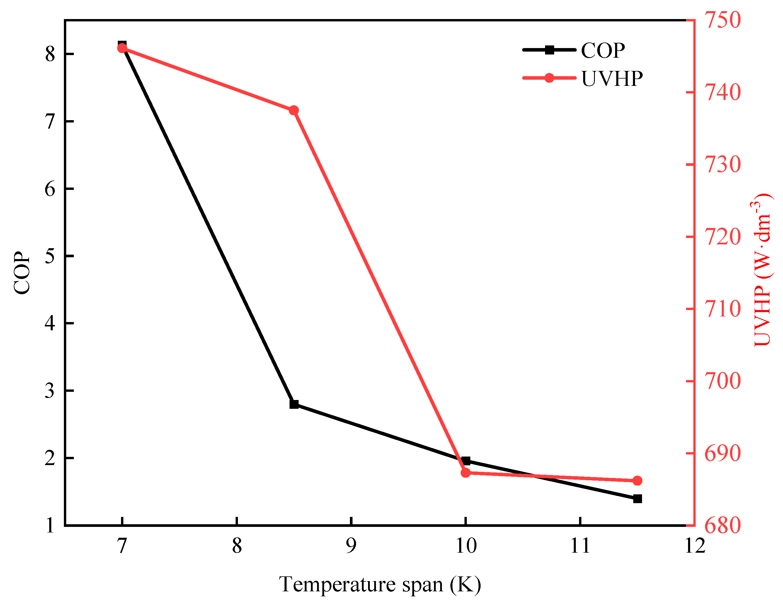
4.2. Heating Performance at Different Temperature Spans

Adopting the control variable method, the temperature of the hot heat exchanger remained constant at 30 °C while the temperature of the cold heat exchanger rose successively from 18.5 °C to 23 °C with intervals of 1.5 K at the same electric field intensity of 125 M V · m 1 and the same cyclic period of 8 s. As seen from Figure 9, COP decreases with the increase in the temperature span, and the largest COP reaches 8.13. Generally, the COP for air-conditioning using vapor compression refrigeration in heating mode is approximately 4.0–6.0 [26]. However, an EC heat pump with a volume of cubic millimeter level can achieve a COP of 8.13 at a temperature span of 7 K, indicating that the EC heat pump has unlimited potential in the development of heat pumps. UVHP also decreases with the increase in temperature span. A maximum of 746.1 W · d m 3 is obtained at the temperature span of 7 K.
When the temperature span successively increases from 7 K to 11.5 K, the UVHP decreases by 1.16%, 6.8%, and 0.17%, respectively, while COP decreases most when the temperature span changes from 7 K to 8.5 K. COP depends on the relative size between Q h and Q c , while there are two variables in Formula 16 that determined the size of UVHP, i.e., T heat T h and u f . To analyze the effect of temperature span only, u f was the same for different cycles. Hence, the differential form of Q h can be written as d Q h = C · d ( T heat T h ) ; C is constant coefficient. The differential form of Q c is d Q c = C · d ( T c T cold ) ; C is also a constant coefficient. As the temperature of the cold heat exchanger decreased equally, T cold varied with T c and then caused T heat T h to change because the fluid’s temperature at the end of the previous cycle always affected the next cycle. 
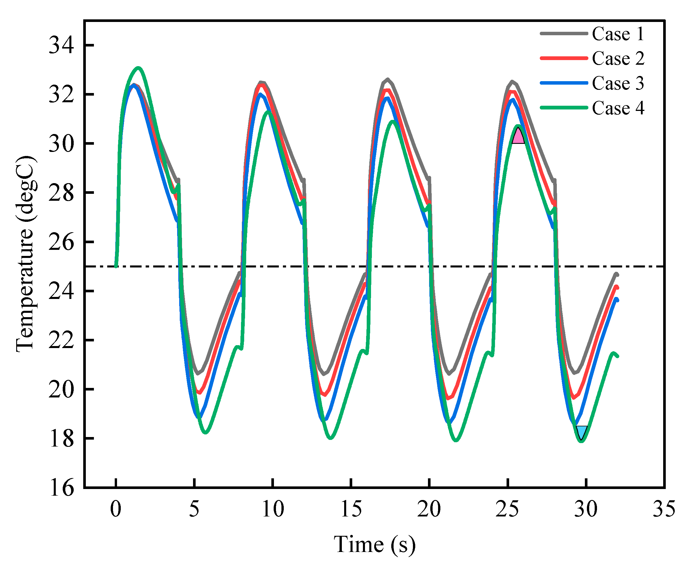
Figure 10 presents the temperature variation trend of the fluid at four different cases shown in Table 3. Taking Case 4 as an example, the red and blue shadows in the figure represent the integral regions of Q h and Q c , respectively. After the cycle tended to be stable, T heat T h and T c T cold decreased with the increase in temperature span, thus leading to the decrease in both heat production Q h and cooling capacity Q c . However, Q c decreases more as COP decreases with the increase in temperature span.
It is known that only the EC device was simulated in COMSOL Multiphysics. Figure 9 shows that only in Case 1 does the fluid that finishes the cycle end up with a temperature close to the original temperature of the EC device, which demonstrates that Case 1 is the most ideal cycle among the four cycles. 
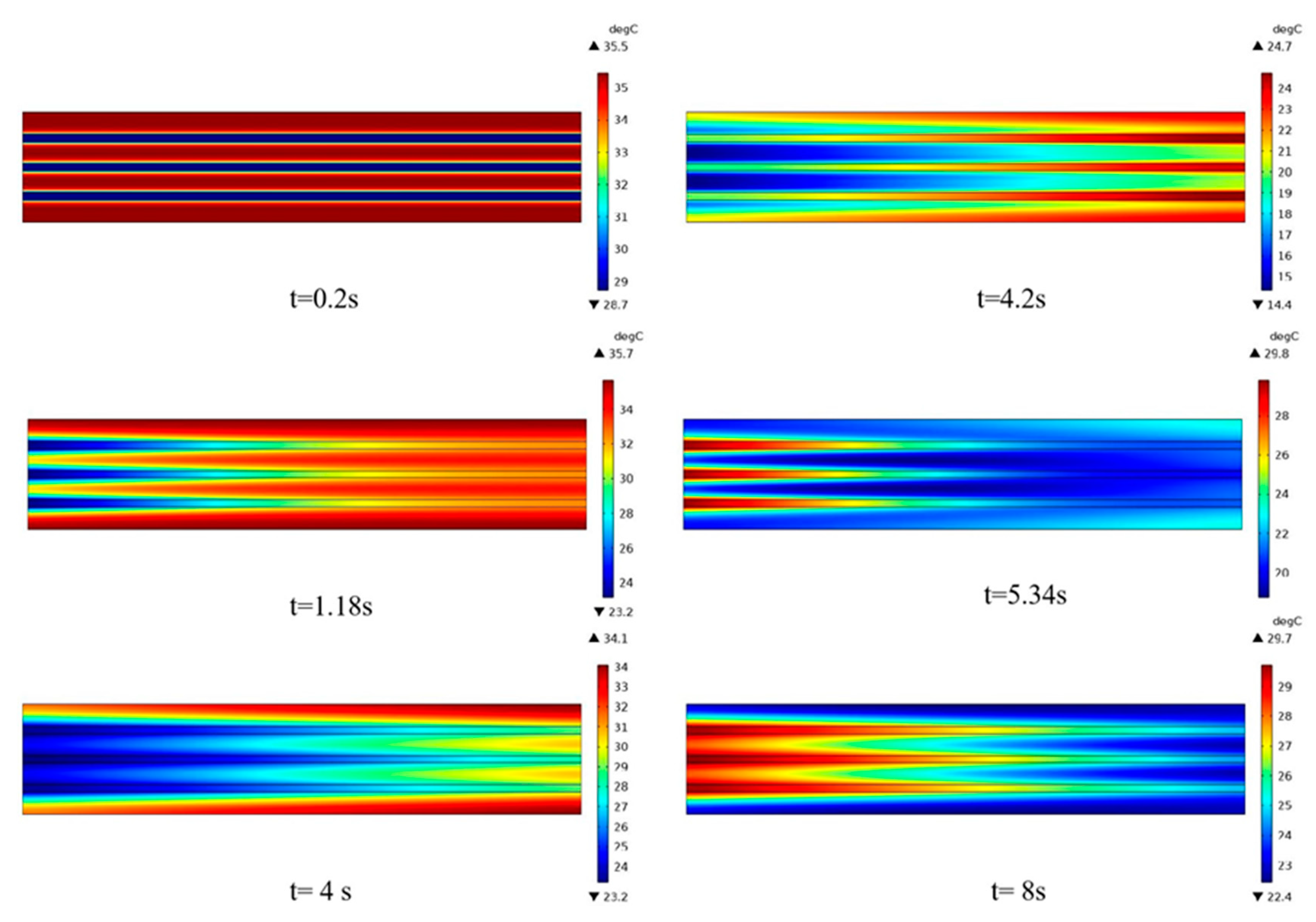
Figure 11 shows the temperature contour of the center plane of the EC heat pump in a complete cycle at Case 1. Among them, 1.18 s and 5.34 s are the highest and lowest moments of the fluid domain’s temperature in the cycle, respectively. The temperature on the left side of the EC material dropped more than that on the right side, and the temperature of the EC material in the middle position dropped more than that on the upper and lower sides after the end of the first half of the cycle. When it comes to the second half of the cycle, the same situation of temperature inhomogeneity happens again. For the layered EC heat pump device, the temperature imbalance between left and right is normal, but the temperature imbalance between upper and lower should be minimized to utilize the heat production and cooling capacity of the EC material most effectively. Therefore, increasing the number of layers of EC material is expected to ensure sufficient heat transfer between fluid and EC material. Hence a four-layer EC heat pump is further simulated at the same operating conditions of Case 1.
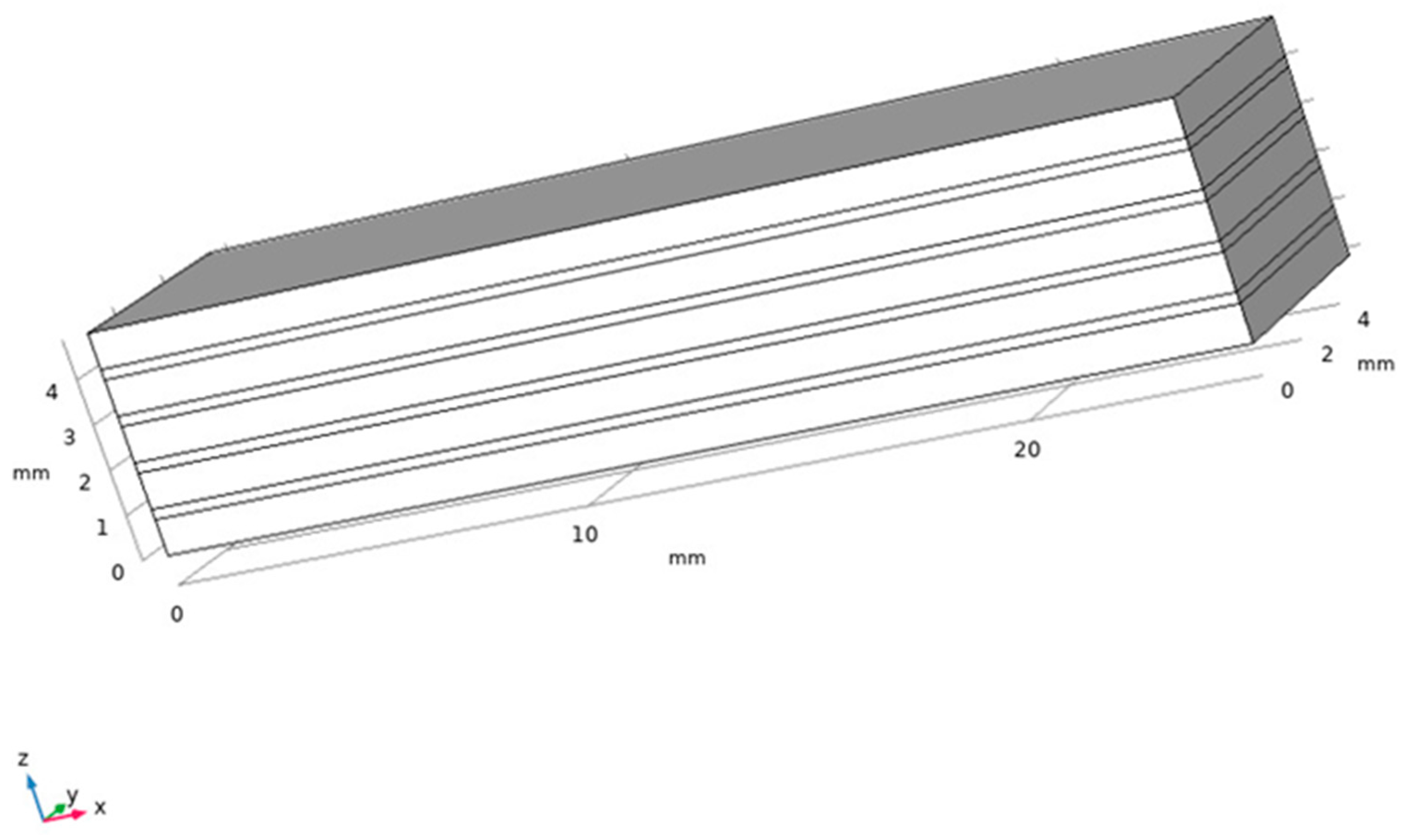
The structure of the four-layer EC heat pump is shown in Figure 12. By changing the relative height of the EC material layer and the fluid layer while keeping the total height of the EC heat pump unchanged, the EC material layer’s and fluid layer’s thickness are 0.8 mm and 0.225 mm, respectively. The length and width of the device are still 25 mm × 5 mm, respectively.
The comparison of the heating performance between the four-layer EC heat pump and the three-layer EC heat pump is exhibited in Table 4. As can be seen from the table, the performance of the four-layer EC heat pump is significantly improved compared to the three-layer EC heat pump, with COP increasing by 25.46% and UVHP increasing by 28.45%. Therefore, the number of layers of the EC heat pump can effectively improve the heating performance due to the increase in heat transfer area. Hence, increasing the number of layers of the EC heat pump can be considered when designing the actual EC heat pump without increasing the material cost.

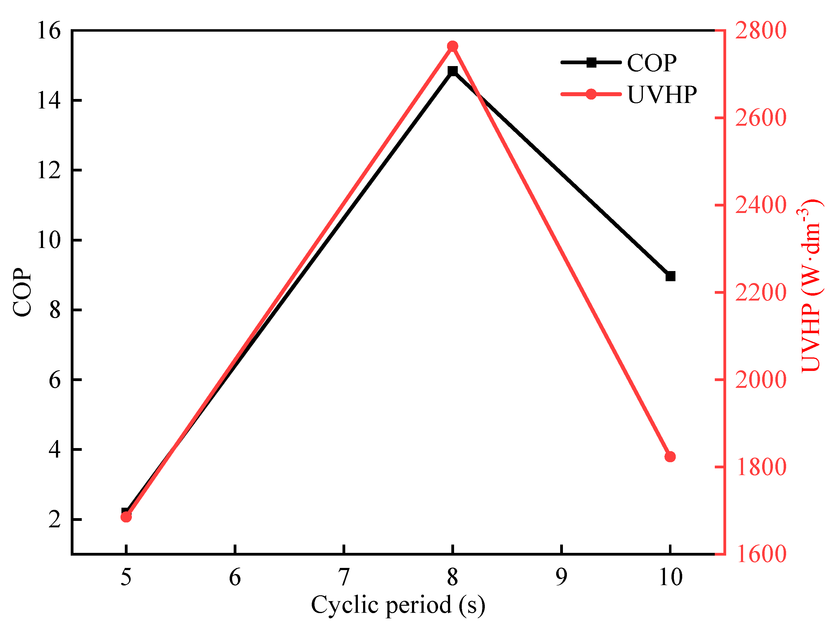
4.3. Heating Performance at Different Cyclic Periods

The cyclic period has a significant effect on the heating performance of the device. It has been tested that the whole simulation will fall into an unstable state when the cyclic period is less than 5 s. Therefore, the cyclic periods set in this study are all more than 5 s, and the time of every simulation contains at least four cycles to ensure cycle stabilization. Moreover, the electric field intensity is fixed at 150 M V · m 1 , and the temperature span is 10 K.
As illustrated in Figure 13, the COP and UVHP of the heat pump reach maximum and minimum values at the cyclic period of 8 s and 5 s, respectively. 
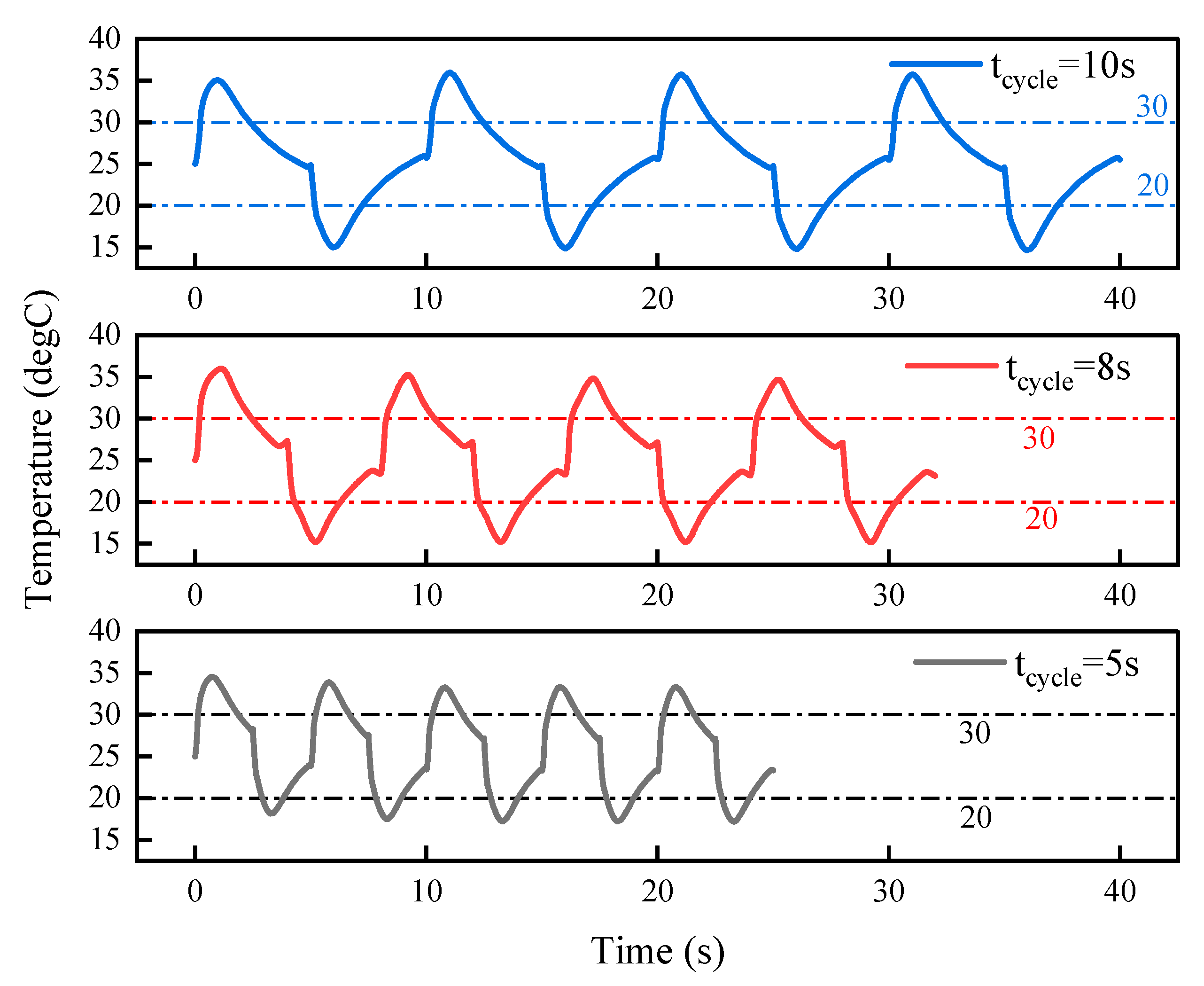
Figure 14 presents the temperature variation trend of fluid at different periods. It can be seen from the figure that the cycle is closest to the ideal cycle at the cyclic period of 10 s because the fluid’s temperature at the end of the cycle is closest to the initial temperature of the device. However, the COP and UVHP of the heat pump at the cyclic period of 10 s are not the best. Since the temperature span and fluid velocity are certain, heat transfer time is the main factor that affects the heat transfer between the fluid and the EC material. After the cyclic period increases, the corresponding heat transfer time between the fluid and the EC material increases, making fluid and EC material transfer heat more adequately. Thus, T heat T h becomes larger when the cyclic period increases from 5 s to 8 s, which makes the heating capacity increase. However, the COP and UVHP of the heat pump decrease, on the contrary, as the cyclic period continues to increase, which is because the heat production of the ECE is finite under the same electric field, and no excess heat could be exchanged with the fluid even if the heat transfer time increases further. Thus, a longer cyclic period can ensure that the fluid returns to the initial state after the end of the cycle, but it cannot guarantee that the performance of the heat pump is the best.

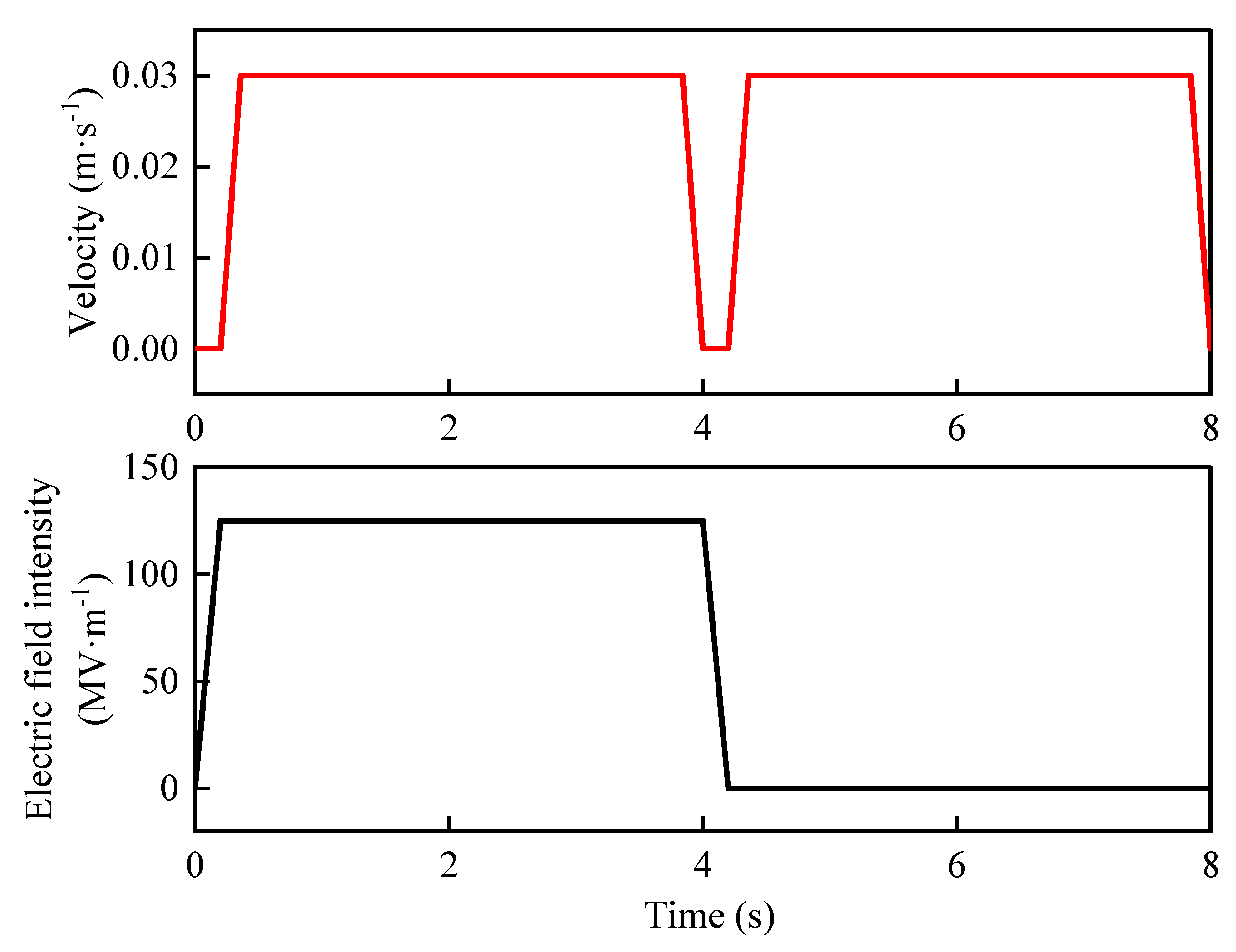
4.4. Heating Performance in Different Electric Fields

In this study, we investigate the influence of electric field intensity on the heating performance of the EC heat pump while keeping the cyclic period and temperature span constant. The changing trend of electric field intensity and fluid velocity in each cycle is shown in 
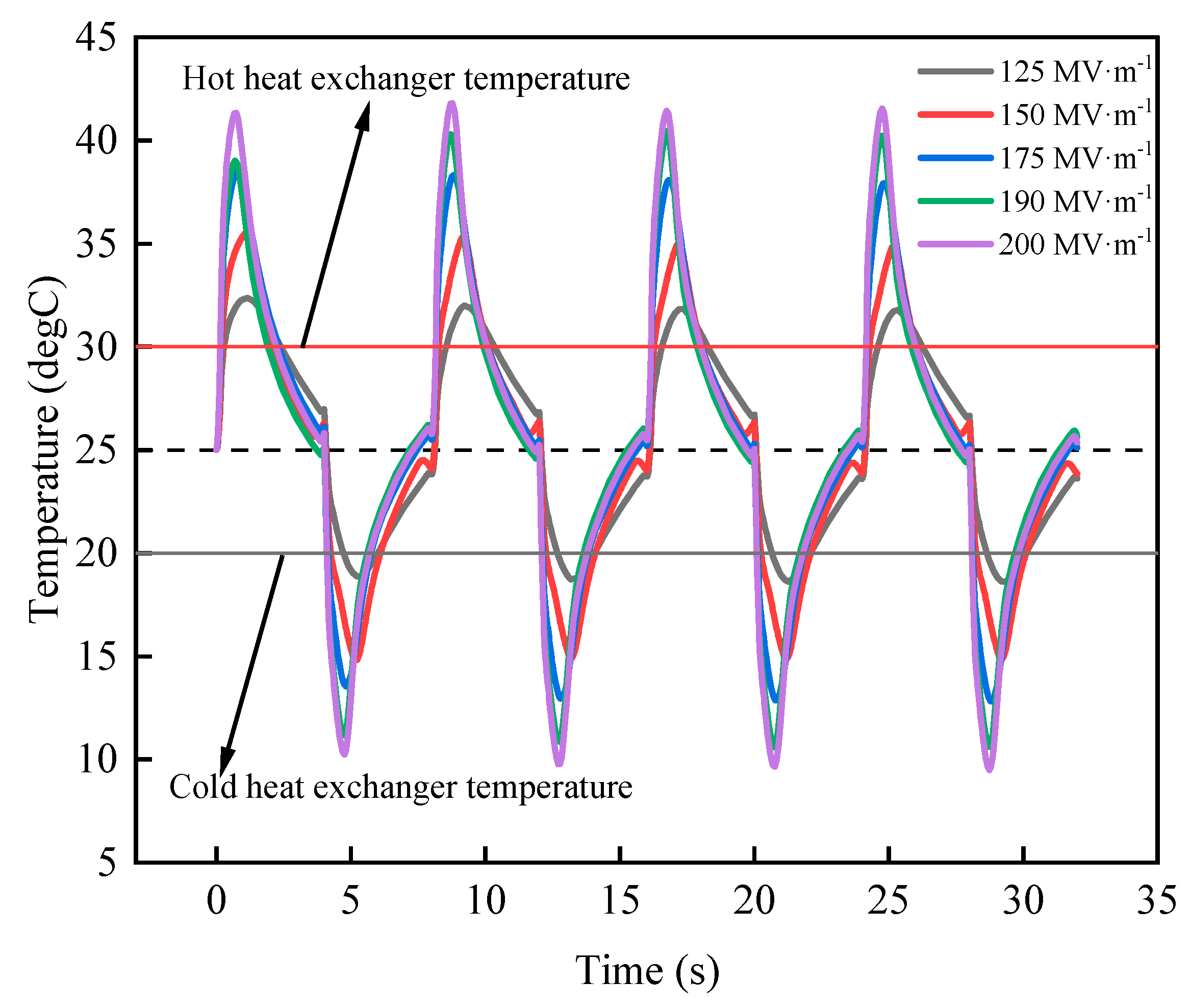
Figure 15. The temperature change of the EC material under different electric field intensities is illustrated in Figure 16. The temperatures of the cold and hot heat exchangers are settled at 20 °C and 30 °C, respectively.
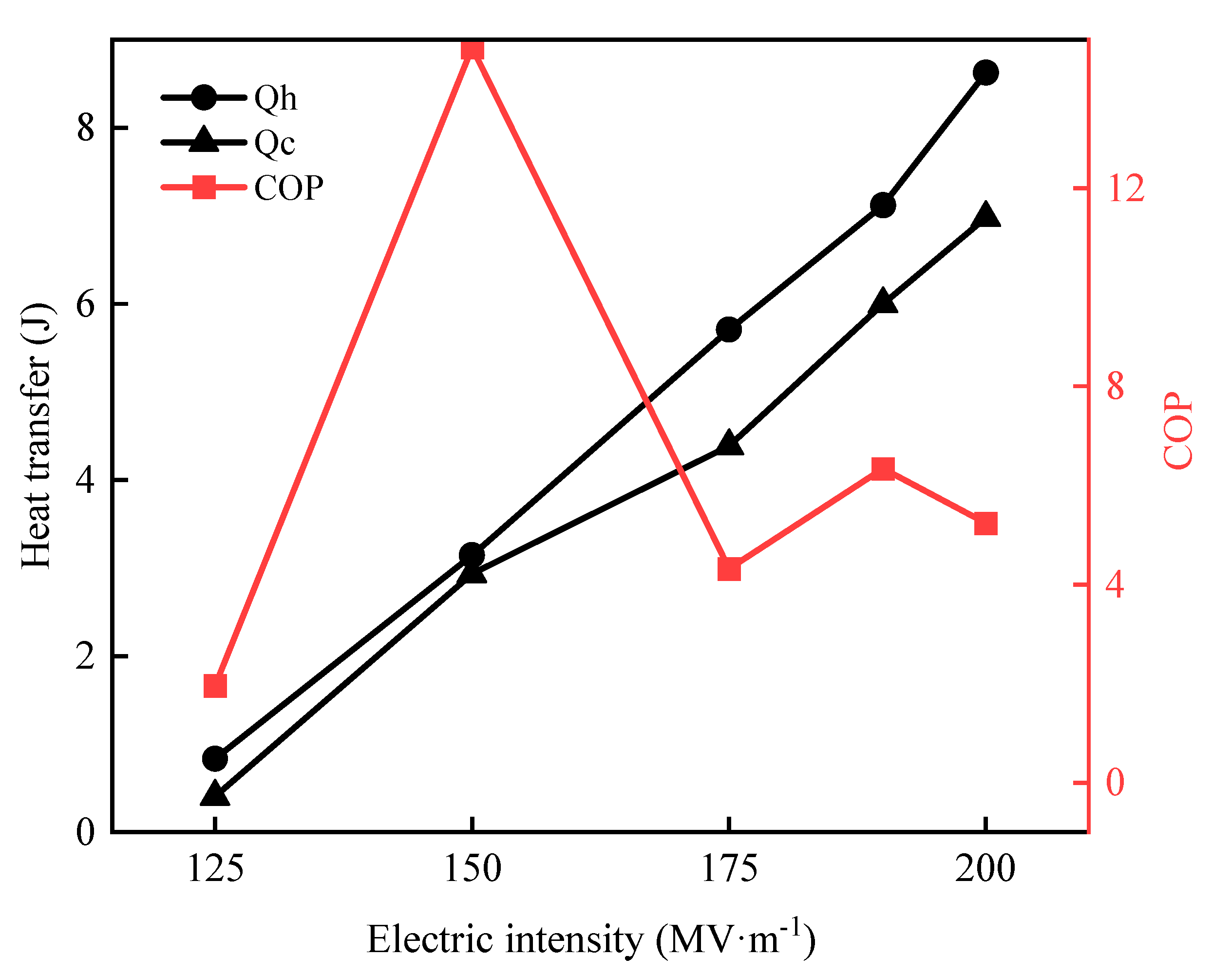
As exhibited in Figure 16, a higher electric field can induce larger ECE so that the temperature change of the EC material becomes more intense. Consequently, the values of Q h and Q c will be larger because the fluid exchanges more heat with the EC material, which is consistent with the variation trend of Q h and Q c depicted in Figure 17. However, COP fluctuates with the increase in electric field intensity and reaches the maximum when the electric field intensity is 150 M V · m 1 .
Figure 16 shows that the temperature of the EC material after a complete cycle is only closer to room temperature at 175 M V · m 1 and subsequent electric field intensities. Meanwhile, the temperature of the EC material at the end of a cycle is lower than room temperature when the electric field intensity is less than 175 M V · m 1 , limiting the temperature lift of the first half period of the next cycle. It can be seen from the figure that this phenomenon has a larger effect when the electric field intensity is 150 M V · m 1 so that Q h becomes smaller and is adjacent to Q c , making COP bigger than the others. When the electric field is 125 M V · m 1 , COP is smaller because the ECE is smaller, and the corresponding heat transfer is less. Therefore, different electric field intensities will affect the overall heat transfer under the same cyclic period and temperature span, which is related to whether the parameters are the most perfect fit. For this reason, proper coordination between the electric field and other parameters is needed to obtain a perfect cycle when designing an EC heat pump.
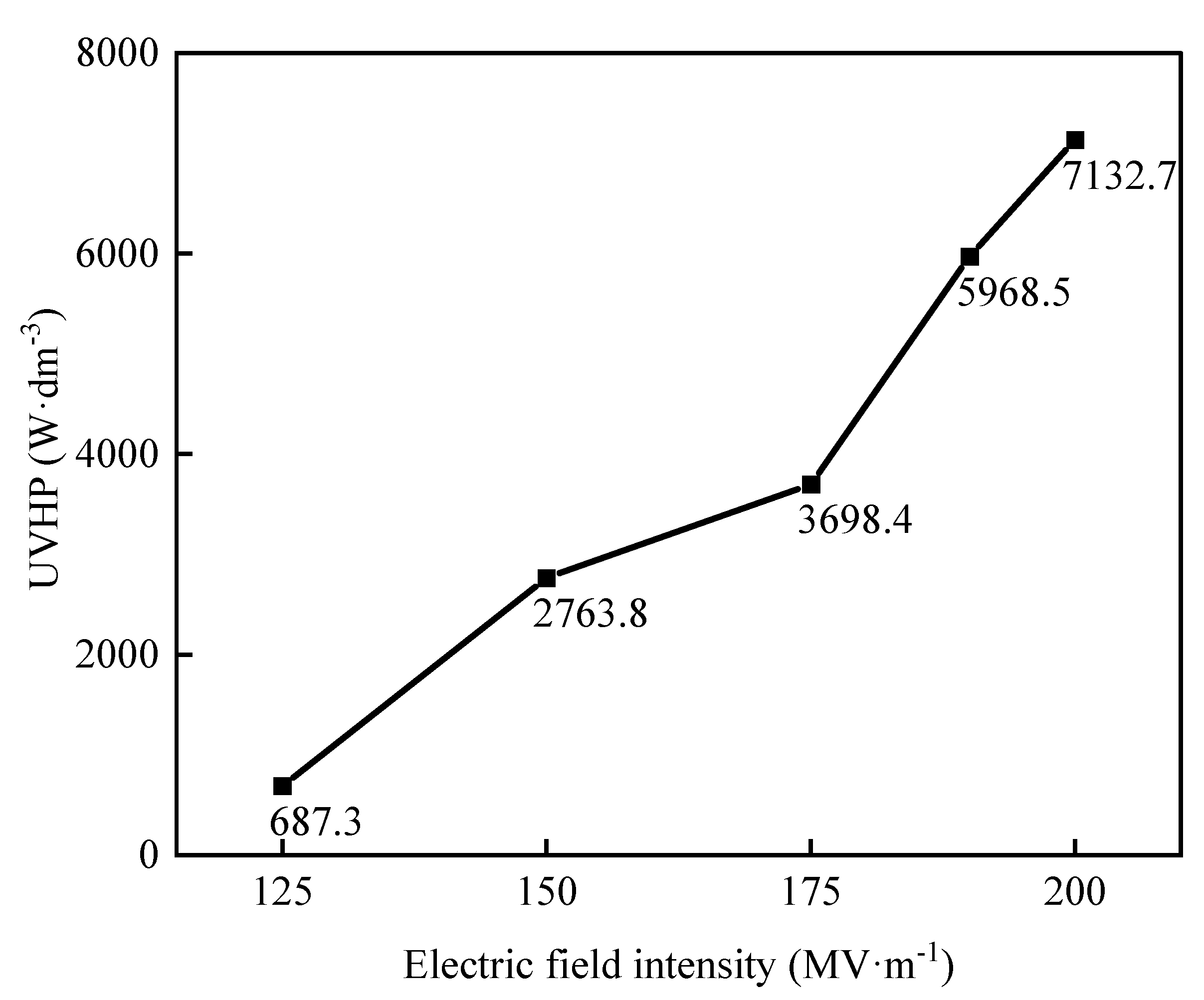
As shown in Figure 18, UVHP shows a different trend. It increases with the electric field intensity in general. Moreover, the growth rate of UVHP is increasingly larger with the increase in electric field intensity. When the electric field intensity increases from 175 M V · m 1 to 200 M V · m 1 , the growth rate of UVHP reaches 92.86%. Within the range of electric field intensity that the EC material can withstand, the bigger the electric field intensity is, the greater the ECE and the temperature variation range of the EC material. In this way, the fluid can also obtain more heat through heat transfer. On the other hand, the temperature of the cold and the hot heat exchangers is invariable, so the temperature difference between the fluid and the terminal becomes larger. According to Formula (16), the greater the temperature difference, the greater the heating power.

5. Conclusions

This paper designed an EC heat pump with highly efficient heat transfer, which is possible to apply in an actual application scenario because of its simple structure. The introduction of negative EC material and Gallium-based liquid metal make the designed EC heat pump system better and more efficient. Different comparative simulation experiments using the control variable method were carried out in COMSOL Multiphysics. COP and UVHP were used as evaluation parameters to measure the performance of the EC heat pump. The principle for the different results was analyzed in detail to give reasonable optimization strategies and provide important guidance for subsequent studies of EC heat pumps. The schemes for optimizing the design of the EC heat pump were given based on the simulation results. The results are as follows:
  • With high thermal conductivity and a low melting point, Gallium-based liquid metal is the new optimum selection for an intermediate heat-carrying medium. COP was up to 14.84, and UVHP was up to 2763.8 W · d m 3 when Gallium-based liquid metal was used as heat transfer fluid under the same operating conditions with other fluids.
  • The heating performance of the EC heat pump decreased as the temperature span increased gradually. The maximum COP of the EC heat pump reached 8.13, and the maximum UVHP reached 746.1 W · d m 3 at a temperature span of 7 K. Furthermore, the performance of a four-layer EC heat pump under the same conditions with Case 1 was studied, and the UVHP increased by 28.45% and COP increased by 25.46% due to the increase in heat transfer area.
  • At a constant temperature span, the maximum COP and UVHP of 14.84 and 2763.8 W · d m 3 , respectively, were obtained at a cyclic period of 8 s.
  • According to the results, UVHP increased gradually with the increase in electric field intensity, and the maximum UVHP reached 7132.7 W · d m 3 at the electric field intensity of 200 M V · m 1 , while COP peaked at 14.84 when the electric field intensity was 150 M V · m 1 .
In summary, the present work reported a simple-structured EC heat pump using Ga-based liquid metal with high thermal conductivity that could achieve highly efficient heat transfer and confirmed its potential for a practical EC heat pump. The overall heating performance of the EC heat pump is closely related to the optimal match among each parameter like electric field intensity, cyclic period, temperature span, electric field intensity, number of layers of the EC heat pump, and so on. Due to the limitation of the EC material, only a small number of EC devices can be studied. In the future, a library in which the different optimal fits of different parameters are listed could be established to offer guiding suggestions for researchers. Furthermore, researchers could devote themselves to developing calculation models in software of different EC materials to promote the advanced development of EC refrigeration or heat pump technology.

Author Contributions

Conceptualization, M.W.; Methodology, Y.Z. (Yangjun Zhang); Software, Z.A.; Validation, X.S.; Writing—original draft, Y.Z. (Yawei Zhu); Writing—review & editing, P.S. All authors have read and agreed to the published version of the manuscript.

Funding

This research was funded by the National Natural Science Foundation of China grant number 51906015. This research was funded by the National Natural Science Foundation of China grant number 52276027. This research was funded by the National Natural Science Foundation of China grant number 52006009. This research was funded by the National Natural Science Foundation of China grant number 52202434. This research was funded by the State Key Laboratory of Automotive Safety and Energy grant number KFY2228. This research was funded by the China Postdoctoral Science Foundation grant number 2022M720424. The APC was funded by 51906015.

Data Availability Statement

Data sharing not applicable. No new data were created or analyzed in this study. Data sharing is not applicable to this article.

Conflicts of Interest

The authors declare no conflict of interest.

Nomenclature

VThe volume of the EC device, mm3
GGibbs free energy of the EC material, J
TTemperature, K
UEC material’s internal energy, J
SEntropy of the EC material, J · k g 1 · K 1
XStress of the EC material, Pa
DElectric displacement vector, C · m 2
EApplied electric field intensity, M V · m 1
xStrain of the EC material, 1
pPyroelectric coefficient of the EC material, 1
ρ Density of the EC material, kg · m 3
cSpecific heat capacity, J · k g 1 · K 1
tTime, s
PHeating power, W
kThermal conductivity, W · m 1 · K 1
uX-direction fluid velocity, m · s 1
C/C’Constant coefficient
Greek symbols
ρ Density, kg · m 3
Δ Finite difference
Gradient operator
Subscripts
hHot side
cCold side
iSomewhere in the EC material
pPressure, Pa
heatHot fluid
fFluid
Acronyms
COPCoefficient of performance
UVHPUnit volume heating power, W · d m 3
ECEElectrocaloric effect
ECElectrocaloric
MFDMagnetofluidodynamic pump

References

  1. Zhang, Z.; Wang, R.; Gao, Y.; Liu, H.; Liu, L.; Bai, J.; Chen, J. Application status and development prospect of heat pump. Refrig. Air-Cond. 2018, 18, 1–8. [Google Scholar]
  2. ERICA. Kigali Amendment to the Montreal Protocol. Available online: http://conf.mont-realprotocol.org/meeting/mop/mop-28/final-report/Site%20Pages/Home.aspx%EF%BC%8E (accessed on 16 February 2023).
  3. Shi, J.; Han, D.; Li, Z.; Yang, L.; Lu, S.-G.; Zhong, Z.; Chen, J.; Zhang, Q.M.; Qian, X. Electrocaloric Cooling Materials and Devices for Zero-Global-Warming-Potential, High-Efficiency Refrigeration. Joule 2019, 3, 1200–1225. [Google Scholar] [CrossRef]
  4. Li, Z.; Shi, J.; Chen, J.; Qian, X. Electrocaloric Cooling Materials and Systems: A review and Perspective. J. Refrig. 2021, 42, 1–13. [Google Scholar]
  5. Mischenko, A.; Scott, J.F.; Mathur, N.D.; Zhang, Q.; Whatmore, R.W. Giant electrocaloric effect in thin film PbZr0.95Ti0.05O3. Science 2006, 311, 1270–1271. [Google Scholar] [CrossRef] [Green Version]
  6. Neese, B.; Chu, B.; Lu, S.-G.; Wang, Y.; Furman, E.; Zhang, Q.M. Large electrocaloric effect in ferroelectric polymers near room temperature. Science 2008, 321, 821–823. [Google Scholar] [CrossRef]
  7. Najmi, F.; He, J.; Cremaschi, L.; Cheng, Z.Y. Electrocaloric devices part II: All-solid heat pump without moving parts. J. Adv. Dielectr. 2020, 10, 2050029. [Google Scholar] [CrossRef]
  8. Guo, D.; Gao, J.; Yu, Y.; Santhanam, S.; Fedder, G.; Mcgaughey, A.; Yao, S.; Slippey, A. Design of a Fluid-Based Micro-Scale Electrocaloric Refrigeration System. In Proceedings of the ASME Summer Heat Transfer Conference, Minneapolis, MN, USA, 14–19 July 2013. [Google Scholar]
  9. Kehileche, B. Numerical prediction of thermal performance of an electrocaloric device based on ceramic material. Prz. Elektrotechniczny 2020, 1, 40–44. [Google Scholar] [CrossRef]
  10. Gu, H.; Qian, X.; Li, X.; Craven, B.; Zhu, W.; Cheng, A.; Yao, S.C.; Zhang, Q.M. A chip scale electrocaloric effect based cooling device. Appl. Phys. Lett. 2013, 102, 122904. [Google Scholar] [CrossRef]
  11. Ma, R.; Zhang, Z.; Tong, K.; Huber, D.; Kornbluh, R.; Ju, Y.S.; Pei, Q. Highly efficient electrocaloric cooling with electrostatic actuation. Science 2017, 357, 1130–1134. [Google Scholar] [CrossRef] [PubMed] [Green Version]
  12. Meng, Y.; Zhang, Z.; Wu, H.; Wu, R.; Wu, J.; Wang, H.; Pei, Q. A cascade electrocaloric cooling device for large temperature lift. Nat. Energy 2020, 5, 996–1002. [Google Scholar] [CrossRef]
  13. Jia, Y.; Sungtaek, Y. A solid-state refrigerator based on the electrocaloric effect. Appl. Phys. Lett. 2012, 100, 242901. [Google Scholar] [CrossRef]
  14. Li, Q.; Shi, J.; Han, D.; Du, F.; Chen, J.; Qian, X. Concept design and numerical evaluation of a highly efficient rotary electrocaloric refrigeration device. Appl. Therm. Eng. 2021, 190, 116806. [Google Scholar] [CrossRef]
  15. Shi, J.; Li, Q.; Gao, T.; Han, D.; Li, Y.; Chen, J.; Qian, X. Numerical evaluation of a kilowatt-level rotary electrocaloric refrigeration system. Int. J. Refrig. 2020, 121, 279–288. [Google Scholar] [CrossRef]
  16. Labouvie, E.W. Influence of crystal defects on dielectric properties of rochelle salt. Z. Nat. A 1968, 23, 997. [Google Scholar] [CrossRef]
  17. Greco, A.; Masselli, C. Electrocaloric cooling: A review of the thermodynamic cycles, materials, models, and devices. Magnetochemistry 2020, 6, 67. [Google Scholar] [CrossRef]
  18. Ozbolt, M.; Kitanovski, A.; Tusek, J.; Poredos, A. Electrocaloric refrigeration: Thermodynamics, state of the art and future perspectives. Int. J. Refrig.-Rev. Int. Du Froid 2014, 40, 174–188. [Google Scholar] [CrossRef]
  19. Newnham, R.E. Properties of Materials: Anisotropy, Symmetry, Structure; Oxford University Press: Oxford, UK, 2005. [Google Scholar]
  20. Li, H.; Jiang, Q.; Xu, X.; Lu, D. A new structure of electrocaloric effect refrigeration based on thermal switch and numerical calculation. Cryogenics 2016, 5, 51–56. [Google Scholar]
  21. Tang, J. Investigation on the Flow Manipulation and Motion Actuation of Gallium-Based Liquid Metal. Ph.D. Thesis, University of Chinese Academy of Sciences, Beijing, China, 2016. [Google Scholar]
  22. Wei, C.; Fei, H.; Tian, Y.; An, Y.; Zeng, G.; Feng, J.; Qian, Y. Room-Temperature Liquid Metal Confined in MXene Paper as a Flexible, Freestanding, and Binder-Free Anode for Next-Generation Lithium-Ion Batteries. Small 2019, 15, 1903214. [Google Scholar] [CrossRef]
  23. Wang, H.; Chen, S.; Zhu, X.; Yuan, B.; Sun, X.; Zhang, J.; Yang, X.; Wei, Y.; Liu, J. Phase transition science and engineering of gallium-based liquid metal. Matter 2022, 5, 2054–2085. [Google Scholar] [CrossRef]
  24. Hasan, M.I.; Rageb, A.M.A.R.; Yaghoubi, M. Investigation of a counter flow microchannel heat exchanger performance with using nanofluid as a coolant. J. Electron. Cool. Therm. Control 2012, 2, 35–43. [Google Scholar] [CrossRef] [Green Version]
  25. Lu, S.G.; Rozic, B.; Zhang, Q.M.; Kutnjak, Z.; Li, X.; Furman, E.; Gorny, L.J.; Lin, M.; Malic, B.; Kosec, M.; et al. Organic and inorganic relaxor ferroelectrics with giant electrocaloric effect. Appl. Phys. Lett. 2010, 97, 162904. [Google Scholar] [CrossRef]
  26. Wang, R.; Xu, Z.; Ge, T. Introduction to solar heating and cooling systems. In Advances in Solar Heating and Cooling; Elsevier: Amsterdam, The Netherlands, 2016; pp. 3–12. [Google Scholar]
Figure 1. Positive electrocaloric effect of EC material.
Energies 16 03104 g001
Figure 2. (a) System design of EC heat pump; (b) detailed two-dimensional structure of EC heat pump; and (c) detailed structure of MFD pump.
Energies 16 03104 g002
Figure 3. Schematic diagram of the device principle where the arrows represent the flow direction of the fluid.
Energies 16 03104 g003
Figure 4. Flow chart of EC heat pump performance study.
Energies 16 03104 g004
Figure 5. Grid details and boundary conditions.
Energies 16 03104 g005
Figure 6. The verification of grid independence.
Energies 16 03104 g006
Figure 7. The verification of the numerical model.
Energies 16 03104 g007
Figure 8. COP and UVHP of different fluids at the temperature span of 10 K.
Energies 16 03104 g008
Figure 9. COP and UVHP at different temperature spans.
Energies 16 03104 g009
Figure 10. Temperature variation of fluid under different temperature spans.
Energies 16 03104 g010
Figure 11. Temperature contour of the EC heat pump at Case 1.
Energies 16 03104 g011
Figure 12. Geometric model of the four-layer EC heat pump.
Energies 16 03104 g012
Figure 13. COP and UVHP at different cyclic periods.
Energies 16 03104 g013
Figure 14. Temperature variation trend of fluid at different cyclic periods.
Energies 16 03104 g014
Figure 15. Changing trend of electric field and fluid velocity in one cycle.
Energies 16 03104 g015
Figure 16. Temperature change of EC material under different electric field intensities.
Energies 16 03104 g016
Figure 17. COP at different electric field intensities.
Energies 16 03104 g017
Figure 18. UVHP at different electric field intensities.
Energies 16 03104 g018
Table 1. Properties of P(VDF-TrFE-CFE) terpolymer [15].
EC
Material
ρ(kg·m−3) k(W·m−1·K−1) c(J·kg−1·K−1) Curie
Temperature (T)
P(VDF-TrFE-CFE)18000.21500341
Table 2. Comparison of the properties of various heat transfer fluid [21,24].
Heat Transfer Fluid Specific   Heat   Capacity   ( J · k g 1 · K 1 ) Heat   Conductivity   ( W · m 1 · K 1 ) Density   ( kg · m 3 )
G a 61 I n 25 S n 13 Z n 1 45023.26320
Nanofluid ( A l 2 O 3 )40520.7191086
Water41830.6999.2
Table 3. Four cases of temperature span.
/Case 1Case 2Case 3Case 4
Cold side temperature (°C)2321.52018.5
Hot side temperature (°C)30303030
Table 4. Comparison of heating performance between the four-layer and three-layer EC heat pump.
Number of LayersCOP UVHP   ( W · d m 3 )
Three-layer8.13746.1
Four-layer10.2958.4
Disclaimer/Publisher’s Note: The statements, opinions and data contained in all publications are solely those of the individual author(s) and contributor(s) and not of MDPI and/or the editor(s). MDPI and/or the editor(s) disclaim responsibility for any injury to people or property resulting from any ideas, methods, instructions or products referred to in the content.

