Remaining-Useful-Life Prediction for Li-Ion Batteries

Abstract

This paper aims to establish a predictive model for battery lifetime using data analysis. The procedure of model establishment is illustrated in detail, including the data pre-processing, modeling, and prediction. The characteristics of lithium-ion batteries are introduced. In this study, data analysis is performed with MATLAB, and the open-source battery data are provided by NASA. The addressed models include the decision tree, nonlinear autoregression, recurrent neural network, and long short-term memory network. In the part of model training, the root-mean-square error, integral of the squared error, and integral of the absolute error are considered for the cost functions. Based on the defined health indicator, the remaining useful life of lithium-ion batteries can be predicted. The confidence interval can be used to describe the level of confidence for each prediction. According to the test results, the long short-term memory network provides the best performance among all addressed models.

1. Introduction

In recent years, the growth of electric vehicles has been accelerated under the policy of global carbon reduction. In battery electric vehicles or other types of hybrid electric vehicles, the Li-ion battery is a core component operating as the power source or power transformer. For the battery-driven equipment, the operating effectiveness strongly relies on a reasonable battery quality. Battery quality could be evaluated by measuring the battery internal resistance or temperature. Practically, routine checking usually costs a lot of manpower, and regular maintenance is not suitable for the unexpected cases where failures occur suddenly. In contrast to preventive maintenance, predictive maintenance (PdM) aims to predict the health status of a piece of equipment according to the model built from the measured characteristics such as voltage, current, and temperature [1,2,3]. Thus, the equipment operation can be real-time-monitored, and the demanded operations can be ensured. Predictive maintenance brings with it several advantages such as avoiding unexpected failures, reducing maintenance costs, and executing necessary module replacements more effectively. As the predictive maintenance of Li-ion batteries, the health status can be determined from the learning models so that the sudden failures can be avoided, and the batteries can be effectively operated in a well-defined condition.

Batteries have been used in various energy storage systems. The health management and degradation models of batteries have attracted a lot of attention. Lithium-ion batteries have characteristics such as high energy density, less self-discharge, and long cycle life [4,5,6]. The battery performance degrades throughout its lifetime, which is known as battery aging. Battery aging is irreversible because of various reasons [7], such as the influence of temperature [8,9,10], the increase in internal resistance caused by chemical reactions [11], the battery charging current [12,13], and the series- or parallel-connection of batteries [14]. Due to the characteristics of long lifetime, high density, and light weight, lithium-ion batteries are preferred over other battery technologies in various applications, including electric vehicles, satellites, laptops, and other consumer electronics.

In recent years, the state of health (SOH) and remaining useful life (RUL) have raised many concerns in the study of battery quality [15]. Both SOH and RUL are important indicators to reflect battery health. Typical methods for the evaluation of battery status include the direct measurement method, physical model method, and data analysis method. In direct measurement methods, an open-circuit voltage is applied to calculate the battery capacity [16], and the battery impedance can be measured by electrochemical impedance spectroscopy [17]. Alternatively, in the physical model methods, the battery degradation behaviors are described by an equivalent model developed from the electrochemical mechanism or equivalent circuit [18,19,20]. In [21,22,23], machine learning methods were adopted to train the SOH model through the history data of batteries. Because of the progressive development of machine learning technologies, data analysis approaches have become the main research trends of battery health analyses.

Over the past several years, traditional maintenance strategies of inspection, testing, repair, and replacement have been applied to ensure equipment are in good condition with high availability and service life [24,25,26]. Basically, the maintenance will not be activated unless a fault occurs. This seeing-is-believing policy could result in significant costs in manpower, time, or money in fault recovery. To improve maintenance effectiveness, the maintenance strategy has gradually changed to the so-called prevention maintenance. For example, a time-based maintenance is in accordance with a pre-defined time routine [27]. However, the maintenance periods are usually varied subject to the working conditions in different devices. In another way, a condition-based maintenance was proposed, where certain thresholds are set for the addressed equipment modules [28]. However, the pre-determined thresholds could be conservative and may involve taking a risk in failure prevention [29]. Condition-based maintenance seems to improve the maintenance performance in a certain degree compared with the time-based maintenance. However, there still exists suspicion in the aspect of failure detection in time. With the popularization of monitoring equipment, predictive maintenance becomes more feasible [30]. In [31], a sliding window algorithm was developed to predict the remaining service life of the battery, and the results showed that the error was within 1.5% and the root-mean-square error in predictive replacement can be made in advance within 20 cycles. In [32], a predictive maintenance strategy was proposed for transformers to attain low cost and high reliability. According to the factors of life reduction and fault increase, a failure rate evolution model was proposed. Predictive maintenance aims to effectively predict equipment failures, prevent problems, save unnecessary maintenance costs, and hope to achieve better results than traditional preventive maintenance strategies.

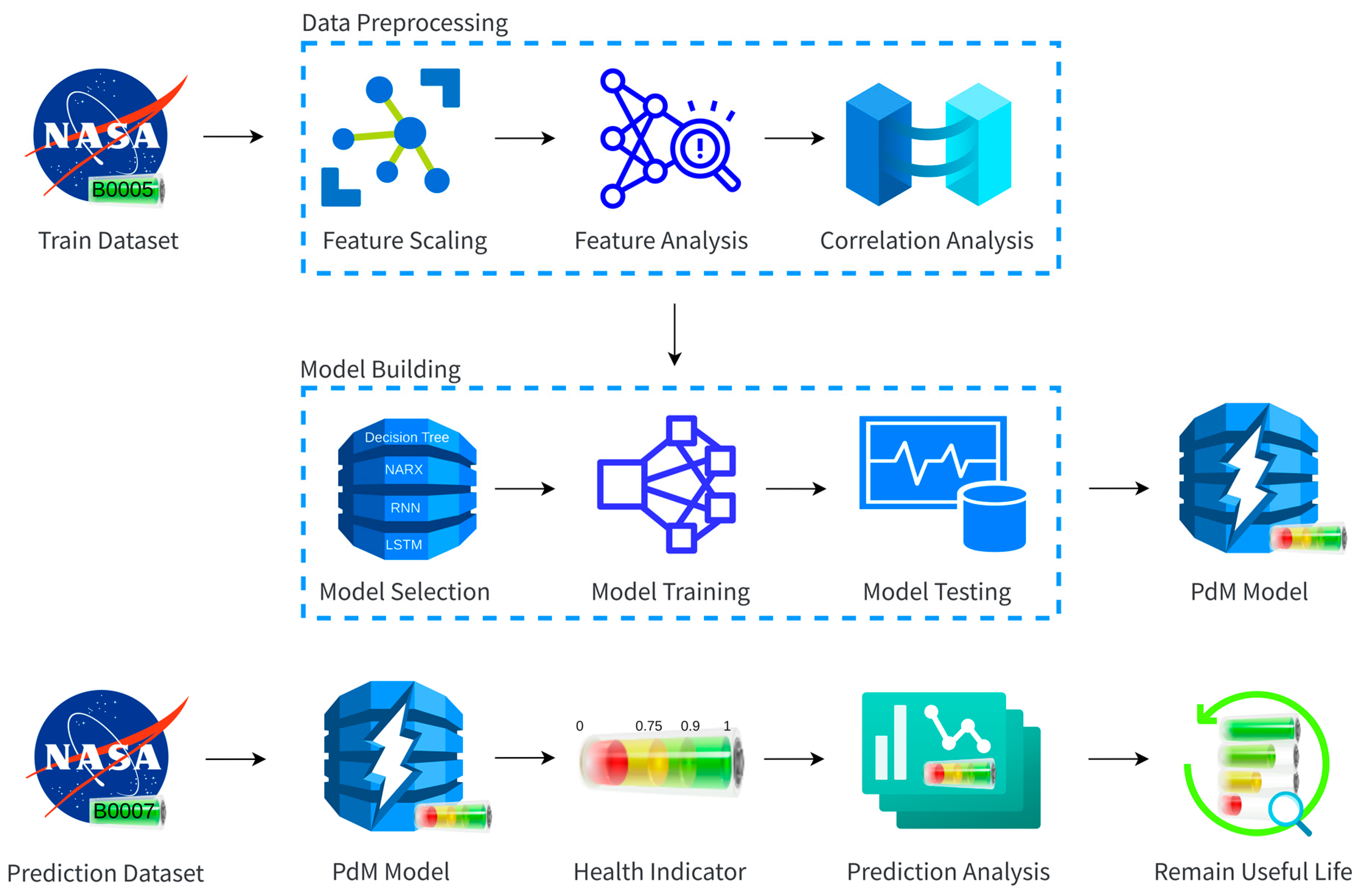
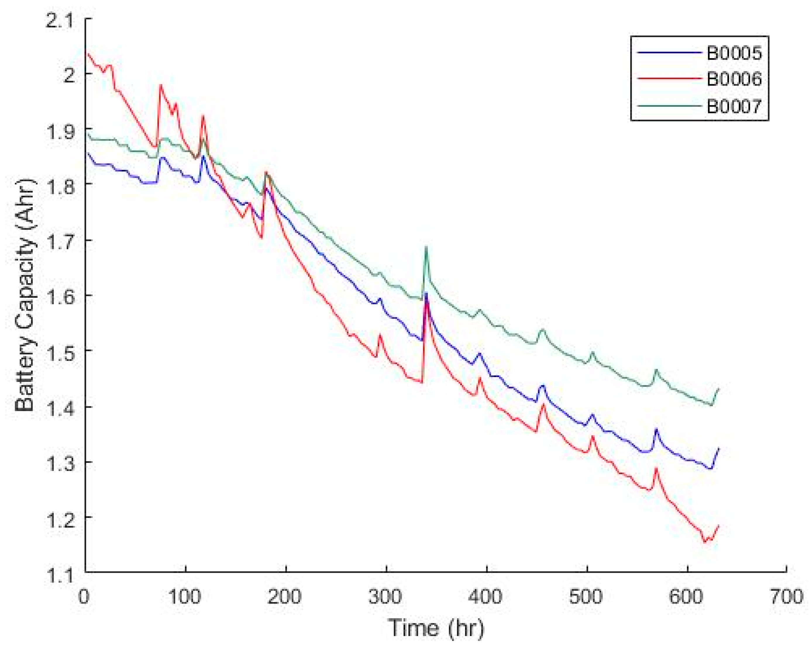
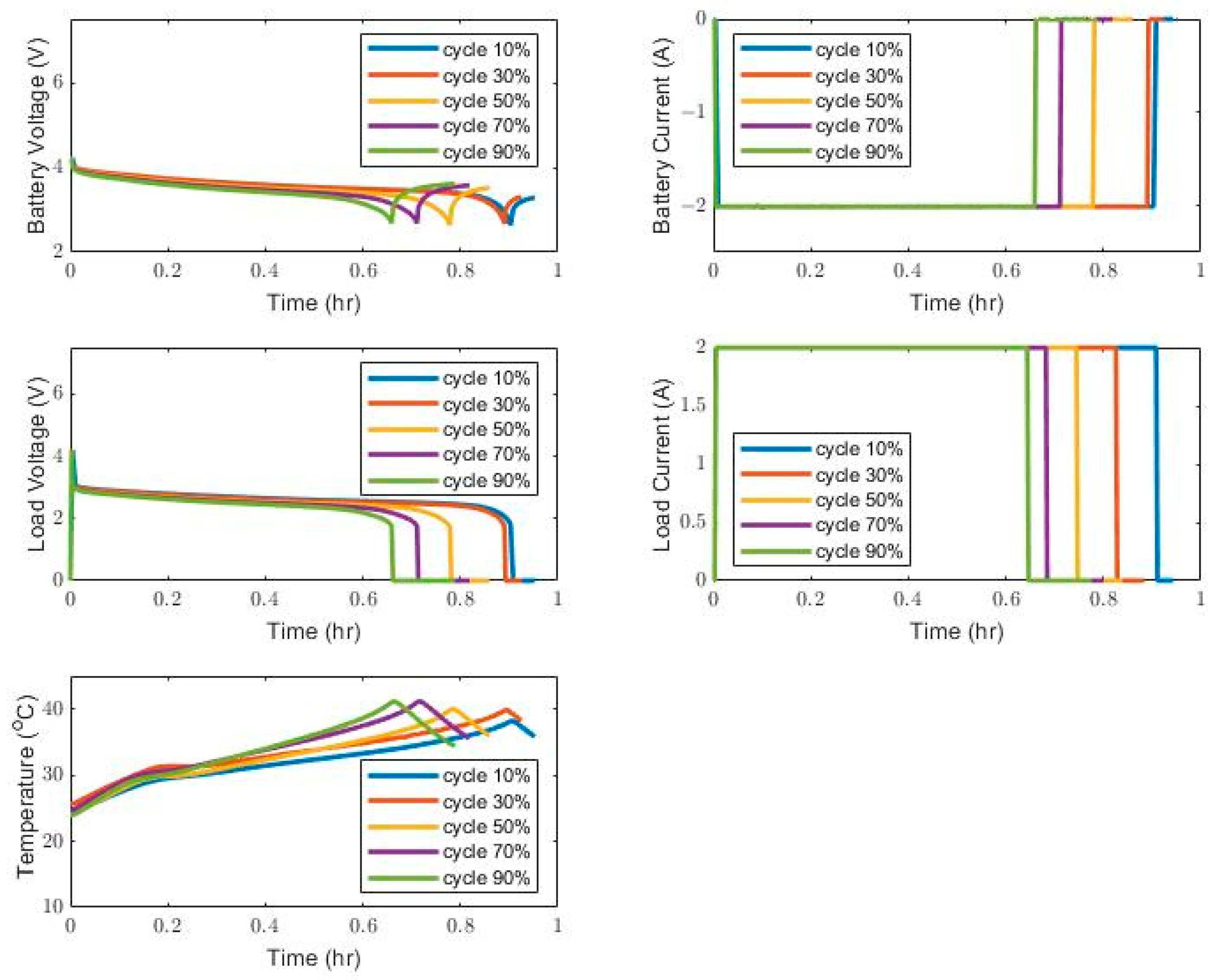
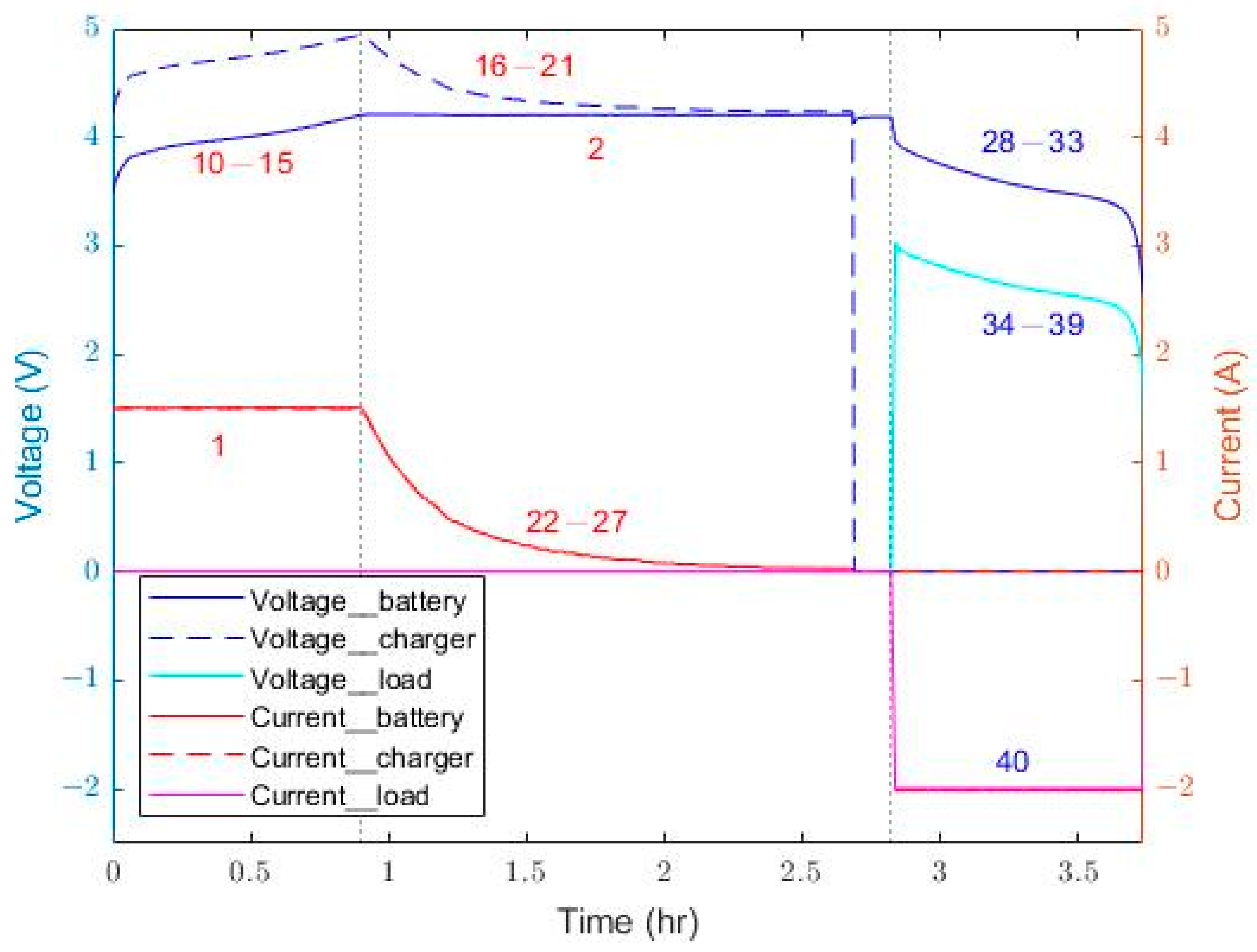
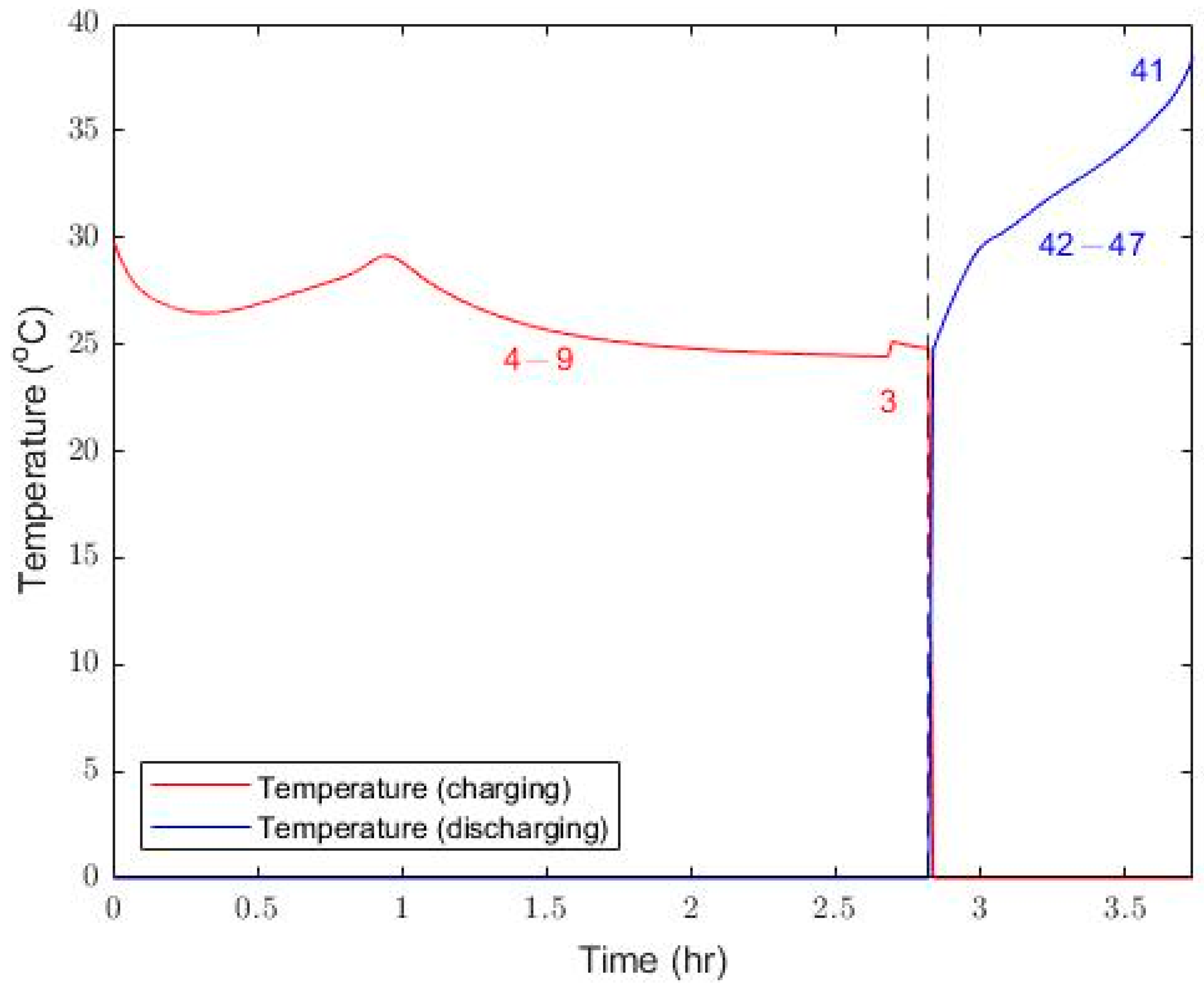
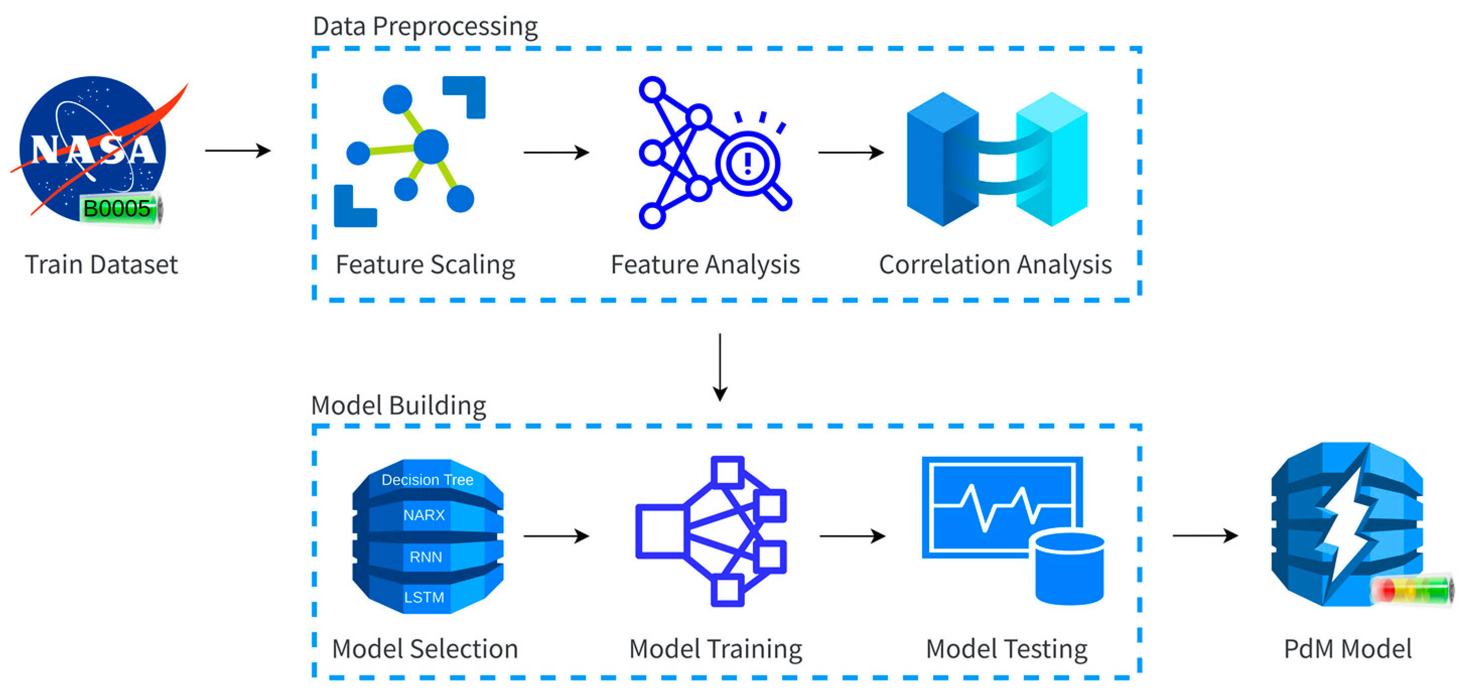
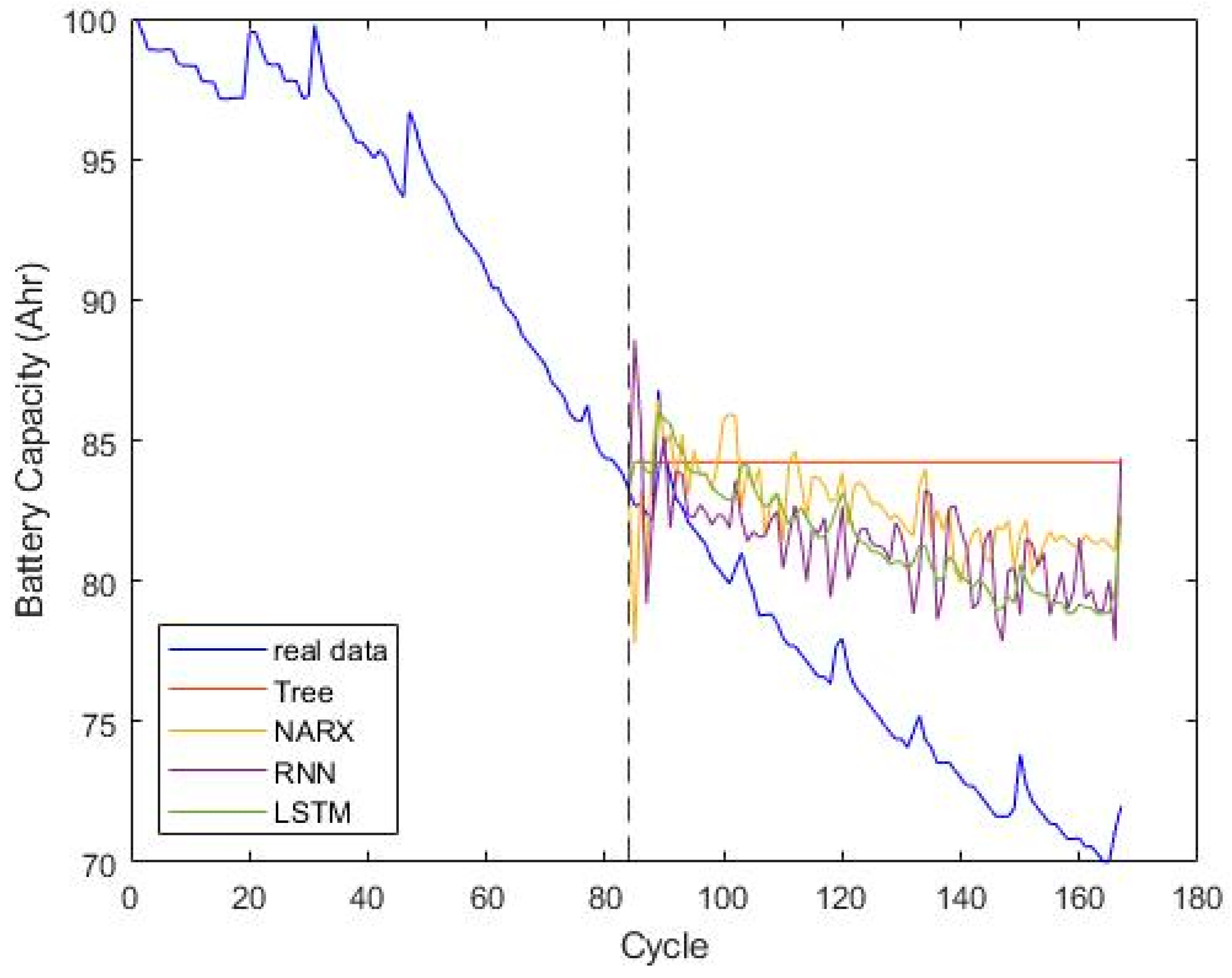
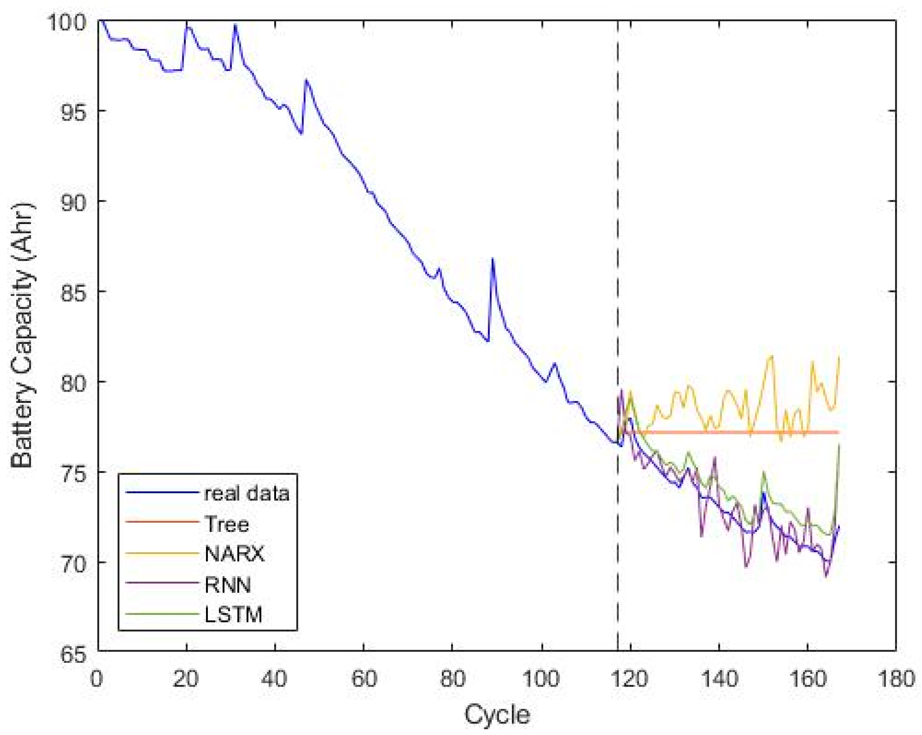
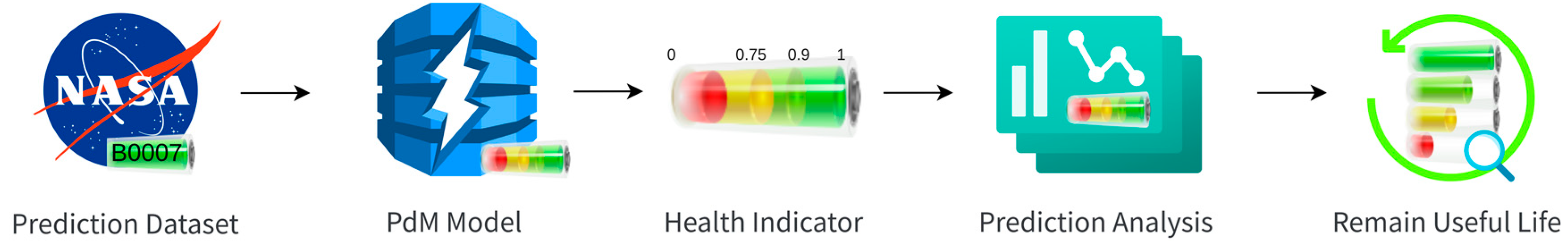
In this paper, the health status of Li-ion batteries is analyzed such that the remaining useful life can be determined in accordance with the learning models. The learning models are generated according to the operating conditions and measured parameters. To build the learning models, the battery features during the charging and discharging processes must be identified. Moreover, the selection of crucial features is performed by using the correlation analysis. Thus, the computation complexity of the model building can be reduced. Finally, the remaining useful life of Li-ion batteries can be predicted. In this paper, the NASA battery dataset is adopted as the real measurements. From the analysis results, the predicted RUL of Li-ion batteries is basically consistent with the trend of the real data. The whole analysis procedures, including the feature selection, correlation analysis, model building, and prediction analysis, addressed in this paper could be helpful for the predictive maintenance of Li-ion batteries in practical cases.

2. Properties of Li-Ion Batteries

The operating principle of lithium-ion batteries, a kind of rechargeable battery, mainly relies on lithium ions moving between the positive and negative electrodes. In the stage of charging, lithium ions move from the positive electrode to the negative plate through the electrolyte and separator. While in the discharging state, lithium ions move from the negative electrode back to the positive electrode. Basically, the structures of the positive and negative electrodes remain the same, and the associated electrochemical reactions are carried out because of the Li-ion migration between electrodes.

2.1. State of Charge

The state of charge (SoC), which is valuable information of the battery, represents the remaining available power of the battery, as shown in Equation (1), where $Q$ is the existing battery capacity and $Q_n$ is the rated capacity of the battery [33]. In practice, the available battery capacity depends on the charge and discharge rate, temperature, and aging phenomenon [34,35]. Absolute state of charge and relative state of charge are two popular types of SoCs. Usually, the relative state of charge is in the range of 0% to 100%, from fully discharged to fully charged. The absolute state of charge is counted as the battery is manufactured. A new fully charged battery has an absolute state of charge of 100%, while an aging battery, even if fully charged, cannot reach 100% in different charge and discharge situations.

$$\mathrm{SoC}=\frac{Q}{Q_n}$$

(1)

SoC is a crucial parameter of battery management. It is necessary to pay attention all the time while normally using batteries. Due to the complexity of the structure and the chemical reactions involved during charging and discharging, the state of charge of lithium-ion batteries cannot be directly measured. Alternatively, some methods have been presented to estimate the state of charge according to the internal resistance, open-circuit voltage, temperature, current, etc.

2.2. Methods of Battery Charging

2.2.1. Constant-Current Method (CC)

In the CC charging process, a constant current is applied for battery charging. The associated charging time is related to the magnitude of charging current [36]. In general, charging with a small charging current will result in a longer charging time. On the contrary, if a larger charging current is applied, a shorter charging time is required to attain the necessary battery capacity. However, it is easy for battery charging with large charging current to damage the battery, decrease the battery capacity, and shorten the battery life. It is noted that the battery voltage increases smoothly during the CC charging process.

2.2.2. Constant-Voltage Method (CV)

Operating with the CV charging method, a constant voltage is applied in the charging process. Compared to the constant-current method, the constant-voltage method has the advantages of being a simple circuit and easy to control. However, due to the low battery voltage in the early stage of charging, it is easy to cause excessive charging current. This situation often causes the rise in battery temperature and the deformation of the battery plate, thereby affecting battery life. It is noted that the battery current decreases continuously during the CV charging process.

2.2.3. Constant-Current and Constant-Voltage Method (CC-CV)

The method combined with the CC and CV charging has better charging performance compared to a single CC or CV method. In the early stage, CC charging is adopted to save charging time and avoid excessive charging current. When the battery voltage rises to the set value, it is converted into CV charging. Then, the charging current will gradually decrease. The battery tends to a saturated state such that the phenomenon of battery overcharge and virtual charging can be prevented [36]. An example of the CC-CV charging procedure is shown in Figure 1.

3. Framework for Predictive Maintenance

Predictive maintenance refers to the maintenance before assets or equipment fail according to the operating information received. In this study, the entire framework of the battery maintenance is divided into three stages: data preprocessing, model construction, and the prediction of remain useful life, as shown in Figure 2. In general, the original data need to be normalized before the process of feature analysis. In the stage of model construction, candidate models are selected and trained to validate which ones are appropriate for the used cases. Finally, based on the trained models, the health indicator can be generated, and the consequent remaining useful life can be predicted.

3.1. Dataset

In this study, the open-source Prognostics Data Repository Battery Data Set is adopted [37,38,39]. The used data, provided by NASA, are stored in the mat files, which contains four 18650-model battery data samples, B0005, B0006, B0007, and B0018. Each battery data sample has four columns: type, ambient_temperature, time, and data array [39]. The data type includes the status of battery charging and discharging. The ambient_temperature records the temperature around the testing battery. According to the recorded data, the environmental temperatures are all at 24 °C. The time array corresponds to the time period of the charging and discharging process. The data field contains an array of records including the voltages and currents in the charging and discharging phases. The conditions of the charging and discharging processes are listed as

Table 1. Operating conditions for charging and discharging process.

Cut-Off Voltage (V)		Current (A)		Capacity (Ahr)
Charging	Discharging	Charging	Discharging	Rated	Lower Bound
4.2	2.7	1.5	2	2	1.4

, and the corresponding features are selected as

Table 2. Features of battery charging and discharging operations.

Features	Description
Voltage_b	The battery voltage in the charging stage
Current_b	The battery current in the charging stage
Voltage_c	The charger voltage in the charging stage
Current_c	The charger current in the charging stage
Voltage_l	The load voltage in the discharging stage
Current_l	The load current in the discharging stage
Temperature	The battery temperature in the charging and discharging stages
Capacity	The capacity after charging and discharging cycles
Time	The time stamp including date, hour, minute, second

.

The battery charging and discharging method used in the dataset adopts the CC-CV method introduced in Section 2. According to the operating conditions shown in Table 1, one example of a charging and discharging cycle is shown in Figure 3. The time-based operation in Figure 3 can be divided into three phases, i.e., constant-current charging (CC_C), constant-voltage charging (CV_C), and constant-current discharging (CC_D). A constant charging current of 1.5 A is applied at the beginning of the charging phase. When the battery voltage reaches the cut-off charging voltage of 4.2 V, a constant-voltage mode starts to work. Consequently, when the current continues to drop to 20 mA, the battery reaches the CC_D discharge state.

3.2. Data Preprocessing

In general, before the feature analysis, attention must be given to the collected raw data in many aspects, such as inappropriate data format, missing data, and symbol encoding. The battery dataset provided by NASA has no problems such as missing data and symbol coding. However, the numbers of different batteries happen to not match. By close observation, although the battery capacity has dropped to the lower bound, the data recording is continued. To unify the sampled data, the number of data samples are trimmed to 168 and divided into charging and discharging stages. In this study, the data preprocessing mainly focuses on the scaling to avoid weight bias in building the learning model. In many cases, feature items often have different size ranges that will be misleading in model building.

3.2.1. Feature Scaling

It is often that features are in different ranges. If the raw data are directly used, it will possibly cause excessive bias of the weights upon model building. Typically, feature normalization is applied such that the source data will be proportionally transferred into the interval [0, 1] [40]. For example, let the maximum and minimum number of a data array be $x_{max}$ and $x_{min}$, respectively. The normalized value $x_{i,nom}$ of the input data $x_i$ can be calculated as (2):

$$x_{i,nom}=\frac{x_i-x_{min}}{x_{max}-x_{min}}$$

(2)

3.2.2. Feature Analysis

The capacities of three batteries are shown in Figure 4. The capacity decreases along with the increase in charging and discharging cycles. The reason for the capacity decline is mainly due to the electrochemical reaction during the charge and discharge cycle. During the electrochemical process of lithium ions in the solution, some passive film will be generated on the surface of carbon materials. Consequently, the battery capacity will decrease [41].

With the increase in cycles, the corresponding features mentioned in Table 2 are shown in Figure 5 and Figure 6. According to the recorded data, the total number of charging/discharging cycles is 170. The cycle 10% notation indicates the situation after 17 charging and discharging processes. In the same way, cycle 30% indicates the situation after 51 charging/discharging cycles. In Figure 5, the approach of the battery voltage to the cut-off voltage of 4.2 V is faster along with the increase in cycles. In addition, the drop in the battery current to 20 mA is faster with the increase in charging/discharging cycles. In addition, the peak of the battery temperature occurs earlier with more cycles. Similarly, in the discharging stage, the abrupt changes in battery temperature and battery/load voltages and currents occur earlier along with the increase in cycles. To further explore the useful information behind the raw time-series data, the following metrics are adopted.

The time-domain analysis refers to the fact that the signal changes over time. Typical quantitative metrics are the mean, skewness, kurtosis, shape factor, etc. For example, a set of data is represented as $\left\{x_i\right\}, i=1, 2, \dots , n$, where $n$ is the number of data points. The mean and standard deviation of the dataset can be calculated as (3) and (4), respectively:

$$\overline{x}=\frac{1}{n}{{\displaystyle \sum }}_{i=1}^n{x}_i$$

(3)

$$\sigma =\sqrt{\frac{1}{n}{{\displaystyle \sum }}_{i=1}^n{\left(x_i-\overline{x}\right)}^2}$$

(4)

In addition, the skewness, kurtosis, and shape factor can be used to describe the characteristics of data distribution, summarized in

Table 3. Time-domain metric formula.

Item	Formula
Skewness	$x_{sk}=\frac{\frac{1}{n}{{\displaystyle \sum }}_{i=1}^n{\left(x_i-\overline{x}\right)}^3}{{\left(\frac{1}{n}{{\displaystyle \sum }}_{i=1}^n{\left(x_i-\overline{x}\right)}^2\right)}^{3/2}}$
Kurtosis	$x_{ku}=\frac{\frac{1}{n}{{\displaystyle \sum }}_{i=1}^n{\left(x_i-\overline{x}\right)}^4}{{\left(\frac{1}{n}{{\displaystyle \sum }}_{i=1}^n{\left(x_i-\overline{x}\right)}^2\right)}^2}$
Shape factor	$x_{sf}=\frac{x_{rms}}{\frac{1}{n}{{\displaystyle \sum }}_{i=1}^n\left|x_i\right|}$
Crest factor	$x_{cf}=\frac{\max \left\{x_i\right\}}{x_{rms}}$
Impulse factor	$x_{if}=\frac{\max \left\{x_i\right\}}{\frac{1}{n}{{\displaystyle \sum }}_{i=1}^n\left|x_i\right|}$
Margin factor	$x_{mf}=\frac{\max \left\{x_i\right\}}{{\left(\frac{1}{n}{{\displaystyle \sum }}_{i=1}^n\left|x_i\right|\right)}^2}$

, where $x_{rms}$ represents the root-mean-square value of $\left\{x_i\right\}$. Furthermore, the crest factor, impulse factor, and margin factor are used to check whether there is an impact signal in the data. The existence of an impact signal could be considered as a warning that something has occurred to the devices. In practice, theses three factors are crucial in the discussion of predictive maintenance. The total features with the combination of the factors in Table 2 and Table 3 are shown in

Table 4. Summary of all features.

Item	Description	Correlation
1	time interval of CC charging	●
2	time interval of CV charging	●
3	battery temperature after charging
4	skewness of temperature in charging
5	kurtosis of temperature in charging
6	waveform factor of temperature in charging	●
7	crest factor of temperature in charging	●
8	impulse factor of temperature in charging	●
9	margin factor of temperature in charging	●
10	skewness of battery voltage in charging	●
11	kurtosis of battery voltage in charging
12	waveform factor of battery voltage in charging	●
13	crest factor of battery voltage in charging	●
14	impulse factor of battery voltage in charging	●
15	margin factor of battery voltage in charging	●
16	skewness of charger voltage in charging
17	kurtosis of charger voltage in charging
18	waveform factor of charger voltage in charging
19	crest factor of charger voltage in charging
20	impulse factor of charger voltage in charging
21	margin factor of charger voltage in charging
22	skewness of battery current in charging
23	kurtosis of battery current in charging
24	waveform factor of battery current in charging
25	crest factor of battery current in charging
26	impulse factor of battery current in charging
27	margin factor of battery current in charging
28	skewness of battery voltage in discharging	●
29	kurtosis of battery voltage in discharging	●
30	waveform factor of battery voltage in discharging	●
31	crest factor of battery voltage in discharging
32	impulse factor of battery voltage in discharging
33	margin factor of battery voltage in discharging	●
34	skewness of load voltage in discharging	●
35	crest factor of load voltage in discharging	●
36	waveform factor of load voltage in discharging	●
37	crest factor of load voltage in discharging	●
38	impulse factor of load voltage in discharging	●
39	margin factor of load voltage in discharging	●
40	time interval of discharging	●
41	battery temperature after discharging
42	skewness of temperature in discharging	●
43	kurtosis of temperature in discharging	●
44	waveform factor of temperature in discharging	●
45	crest factor of temperature in discharging	●
46	impulse factor of temperature in discharging	●
47	margin factor of temperature in discharging	●
48	capacity	●

, where there are 48 features. All features refer to their time interval or time instance and are highlighted in Figure 7 and Figure 8, corresponding to the charging and discharging stages, respectively. For example, the notation “1” shown in Figure 7 indicates the first item in Table 4, which is the time interval of CC charging. The rest of the features in Table 4 can be cross-checked from Figure 7 and Figure 8.

3.2.3. Correlation Analysis

Correlation analysis is an analytical technique used to analyze the degree of correlation between feature items. It can extract some crucial features for the consequent model building with less computation complexity. The Pearson correlation, Spearman correlation, and Kendall correlation coefficient are commonly used in correlation analyses [42].

The Pearson Correlation Coefficient is typically used to determine the degree of linear correlation between two sets of data, $\left\{x_i\right\}$ and $\left\{y_i\right\}, i=1, 2, \dots , n$. The correlation coefficient is determined as

$$corr=\frac{{{\displaystyle \sum }}_{i=1}^n\left(x_i-\overline{x}\right)\left(y_i-\overline{y}\right)}{\sqrt{{{\displaystyle \sum }}_{i=1}^n{\left(x_i-\overline{x}\right)}^2}\sqrt{{{\displaystyle \sum }}_{i=1}^n{\left(y_i-\overline{y}\right)}^2}}$$

(5)

The absolute value of the correlation coefficient is less than or equal to one. The higher the value, the closer the relationship between $\left\{x_i\right\}$ and $\left\{y_i\right\}$, as shown in

Table 5. The relationship strength according to the correlation coefficient.

Strength	Positive Correlation	Negative Correlation
Strong	0.5–1	−1–0.5
Moderate	0.3–0.5	−0.5–0.3
Weak	0.1–0.3	−0.3–0.1
Negligible	<0.1	−0.1–0

. The sign of the correlation coefficient represents a positive or negative correlation between $\left\{x_i\right\}$ and $\left\{y_i\right\}$.

In this study, the Pearson correlation coefficient is used to analyze the correlation of the 48 features. After the correlation analysis, the dominant features are selected, as shown by the notation ● in Table 4. In the following, the sorted dominant features are adopted for the building of learning models.

3.3. Model Building

The data provided by the data preprocessing are used for the consequent model building. The process of model building goes through model selection, model training, and model testing, as shown in Figure 9. In the context of predictive maintenance, the method of supervised learning is adopted, where a model is built to regressively predict the battery capacity.

3.3.1. Model Selection

The learning models adopted in this study are briefly explained in the following. Decision Tree is a tree-like structure, starting from a root node, where each inner node represents a test on an attribute, each branch indicates an outcome of the test, and each leaf node stands for a class label. Decision Tree is a non-parametric supervised learning method used for classification and regression. The goal is to create a model that predicts the value of a target variable by learning simple decision rules inferred from the data features. Basically, the learning of decision tress includes the following steps: feature selection, tree generation, and pruning. The selection of features determines which feature to use as a judgment. After deciding the features, it is triggered from the data sample (root node), and the information gain of all features is calculated for the node. The feature with the largest gain is selected and the child node is established, and then the new child node is generated in the same way for each child node until the information gain is small or no features can be selected. Finally, the pruning of the decision tree is applied to avoid the decision tree growing too deep that may result in high computation complexity and possible overfitting.

Nonlinear autoregressive with external input (NARX) is a nonlinear autoregressive model that has exogenous inputs. NARX models relate the current value of a time series to past values of the same series and current and past values of the driving series. The structure of the NARX network generally consists of an input layer, hidden layers, and an output layer. The NARX network has the feedback and memory functions inherited from the input and output delays, such that the prior information can be retained and added to the calculation of the next moment. The Recursive Neural Network (RNN) is similar to the NARX network. In contrast to the NARX model, RNN does not have feedback connections from the output to the input. The feedback connection exists only among the neurons in the hidden layer. The Long Short-Term Memory Network (LSTM) is an extension of RNN, and the hidden layer in RNN is improved to solve the problem of long-term dependencies. The main difference between an LSTM unit and a standard RNN unit is that the LSTM unit is composed of the so-called gates that supposedly regulate better the flow of information through the unit.

3.3.2. Model Training

Before model training, the data are divided into three sets for training, validation, and testing. In supervised learning, the model makes predictions according to the data in the training set. Compared with the differences between the prediction results and actual targets, the model parameters can be progressively adjusted. The validation set is basically used for the validation of the preliminary capabilities of trained models. The hyperparameters such as the depth of the hidden layer and the number of neurons can be further adjusted. In practice, the validation process is not necessary in data partitioning. The performance verification of the trained models can be validated through the unused test set, where the capabilities of prediction and classification are commonly addressed. Considering that the size of NASA battery datasets is limited, in this paper, 70% of the battery datasets are used for model training and the remaining 30% of data are used for model testing [43]. It is reasonable that if more data are available, the outcomes from trained models will approach those of the actual data. From Figure 10 and Figure 11, it can be seen that the prediction outcomes with the 70% training dataset are much better than the counterparts with the 50% training dataset; especially, the predictions from RNN and LSTM are significantly improved, where the prediction trends are close to the real data.

3.3.3. Model Testing

In the previous step, 70% of the dataset are used to build the model, and then the remaining 30% of the data are used in the model testing to verify the established model. The output values of the trained models are point-wisely compared with the actual values to find the loss function. In this study, the measurements of root-mean-square error, the integral of absolute error, and the integral square error are considered. In

Table 6. Comparison of different learning models in model testing.

Model	RSME	IAE	ISE
Tree	0.138	6.082	10.919
NARX	0.185	8.202	13.171
RNN	0.045	1.641	6.433
LSTM	0.038	1.423	4.593

, the RNN and LSTM have a better performance than the outcomes of Decision Tree and NARX. Among all the applied learning models, LSTM has the superiority in all aspects of error metrics.

The decision tree model is used for common regression applications. For time-series data with multiple categories, the prediction capability is limited. In the NARX model, the feedback output can be considered as an extra feature. However, if the information is not effectively denoised, it often causes the wrong judgment. The RNN model has the recurrent characteristics. Theoretically, RNN is suitable for any length of time series data. However, there exists the problems of gradient explosion or gradient disappearance. As a derivative of the RNN model, the LSTM model introduces the design of new memory units and gate controls such as input, output, and forget gates. The problems caused by gradient explosion or gradient disappearance can be solved. In addition, better prediction results can be obtained.

4. Prediction of Remain Useful Life

In the stages of feature analysis and model building, the B0005 and B0006 data are used. After the PdM model is built, new battery data from B0007 are used to validate the prediction performance of the RUL. In this study, without loss of generality, the first 50 cycles of B0007 are considered as the new information. By feeding the new information into the learning models, the remaining useful life can be predicted through a process of prediction analysis. The execution process is shown as Figure 12, where the remaining useful life can be determined from the health indicator.

4.1. Health Indicator

In predictive maintenance, the health indicator (HI) refers to a value that can represent the current health status of the equipment based on some analyses of long-time recorded data. For the Li-ion battery, the state of charge is considered as the health indicator of the battery. In this study, the health index is between 0 and 1, where the value of 1 represents the state of complete health and the value of 0 represents complete failure of the battery. The study in [31] indicates that the degradation will be aggravated if the capacity is lower than 80%. Under this situation, the battery is still workable. However, if the capacity is lower than 70%, the battery degradation becomes severe and the battery is not normally workable. By looking closely at the NASA battery dataset, the data are only recorded to 70% of the rated capacity. In this study, the status of the battery is “good” when the HI is more than 90%, “normal” when the HI is 75–90%, and “bad” when the HI is below 75%.

Taking the first 50 cycles as the operating record of the battery B0007, the associated predictions from different models are shown in Figure 13, Figure 14, Figure 15 and Figure 16. In Figure 13, it can be observed that the predicted battery capacity is 93.87% immediately after the first 50 cycles. According to the previously mentioned metrics about the health status of the battery, the battery is in the “good” status analyzed by the Tree model. Similarly, the predicted health indicators of other learning models, NARX, RNN, and LSTM, are summarized in

Table 7. Health indicators of different models (50 cycles).

Model	HI	Status
Tree	93.87%	good
NARX	95.45%	good
RNN	90.05%	good
LSTM	91.34%	good
Real value	93.84%	good

, where the status “good” is afforded by each model. From the real data of the B0007 battery, the health indicator is 93.84% and the battery is actually in the “good” status. Closely checking the prediction results of Decision Tree, the predicted health indictor seems to be saturated around 80% regardless the increase in cycles. In Figure 14, the NARX model can generate a deteriorating trend more precisely. However, predicted battery capacities lower than 75% exhibit obvious bias compared to the real data. From Figure 15 and Figure 16, the learning models RNN and LSTM can provide better predictions, where the variation in LSTM is smoother than the results from RNN.

4.2. Prediction Analysis

The remaining useful life can be determined according to the calculated health index. Practically, health indicators will gradually drop to zero or certain well-defined values over a period of time, and this time interval is the remaining life [44]. From the NASA dataset, the total number of whole charging/discharging processes is 180. In this study, the cycle number of 180 is considered as the whole life of a testing battery. According to the discussion in Section 4.1, the health indicator below 75% is considered as “bad”. The battery needs to be replaced to maintain the working battery in the health status. Without loss of generality, the behavior during the first 50 cycles is considered as the currently new information of the battery. If the capacity prediction is lower than 75% at a certain cycle, the difference between this cycle and 50 can be considered as the remaining useful life predicted by a certain learning model of interest. For example, the analysis results of LSTM are shown in Figure 17, where the red line is the capacity prediction beyond 50 cycles. From Figure 17, the capacity is below 75% at cycle 126. Thus, the remaining useful life is 76. According to the real data, the remaining useful life is 84. The prediction results with different learning models are shown in Figure 18, and the predicted RULs are summarized in

Table 8. Remaining useful life of different trained models.

Model	HI < 75% (cycle)	RUL (Cycle)	Error Index
			RMSE	IAE	ISE
Tree	na	na	0.164	20.521	44.001
NARX	84	34	0.276	35.113	30.918
RNN	146	96	0.129	16.869	39.781
LSTM	126	76	0.063	7.130	18.249
Real value	136	84

. In Table 8, it can be seen that the RUL obtained from LSTM is closer to the real data compared to other models.

5. Discussion

In this paper, the NASA battery dataset is adopted for the prediction of remaining useful life. The essential properties of Li-ion batteries are briefly introduced such as the state of charge and the current and voltage profiles during the charging/discharging stages. The state of charge is a crucial factor to identify the battery quality such that the battery capacity is particularly selected as one feature in the feature analysis and consequent model building. In addition, possible features are selected from the charging and discharging processes such as the battery current, voltage, and temperature. The feature selection analysis is clearly addressed in this paper, including the correlation analysis. In the model building, several learning methods, Tree, NARX, RNN, and LSTM, are used. In this paper, they are mainly used to analyze which method is more appropriate to the model building based on the addressed dataset. Through the data analysis, the CC-CV charging method is applied in the NASA battery dataset. The information in the dataset is quite complete, including the period of charging/discharging time and the corresponding currents, voltages, and temperatures. Due to the completeness, the NASA battery dataset is very suitable for the health status analysis of Li-ion batteries. However, one drawback is that there are only 4 batteries, each with 170 charging/discharging cycles. Considering the possible prediction bias, confidence intervals are introduced in Figure 13, Figure 14, Figure 15, Figure 16 and Figure 17. The proposed results could be useful for the RUL prediction of Li-ion batteries in other practical cases. In addition, the learning methods may be modified to enhance the prediction performance of battery health in future works.

6. Conclusions

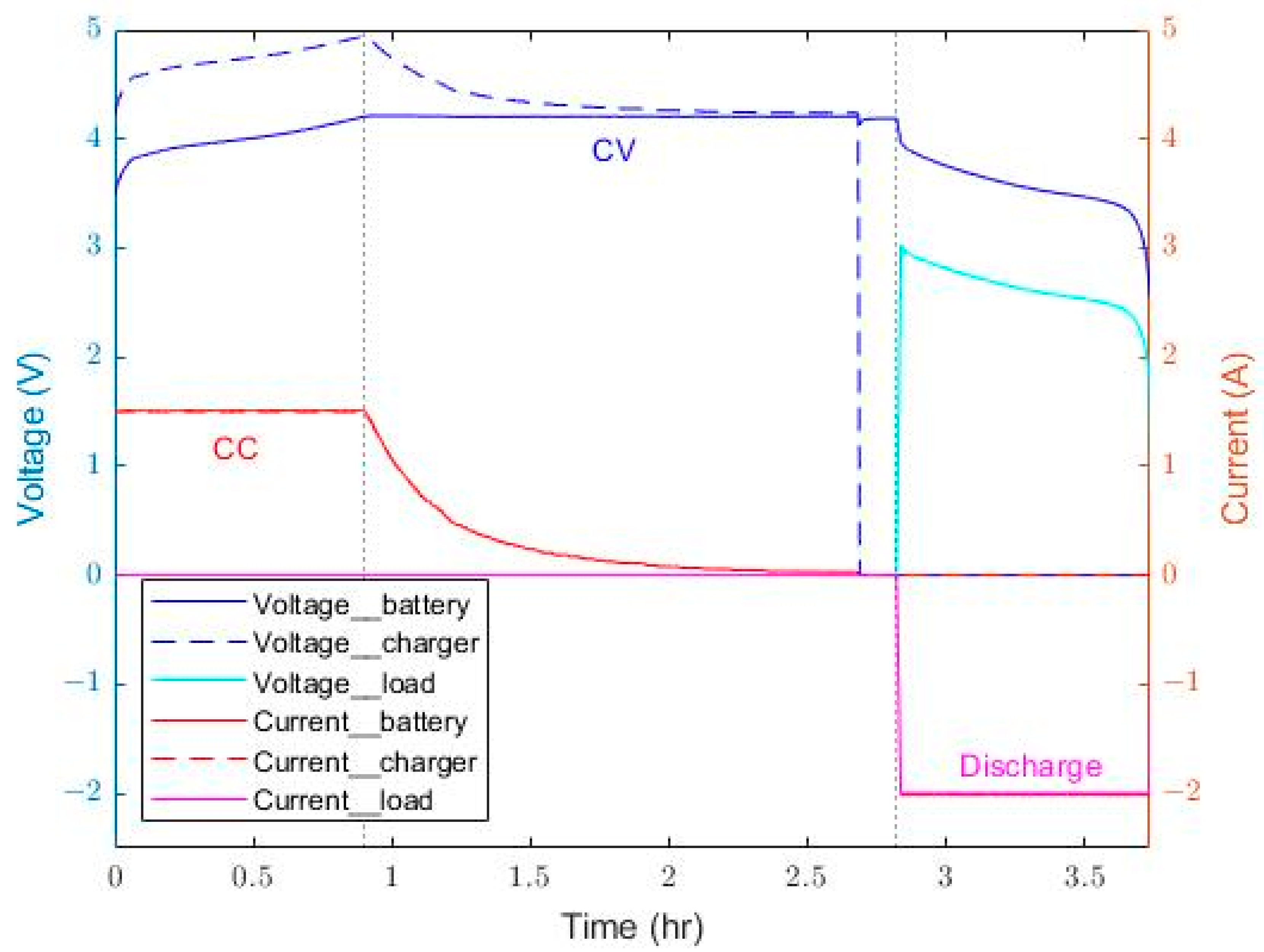
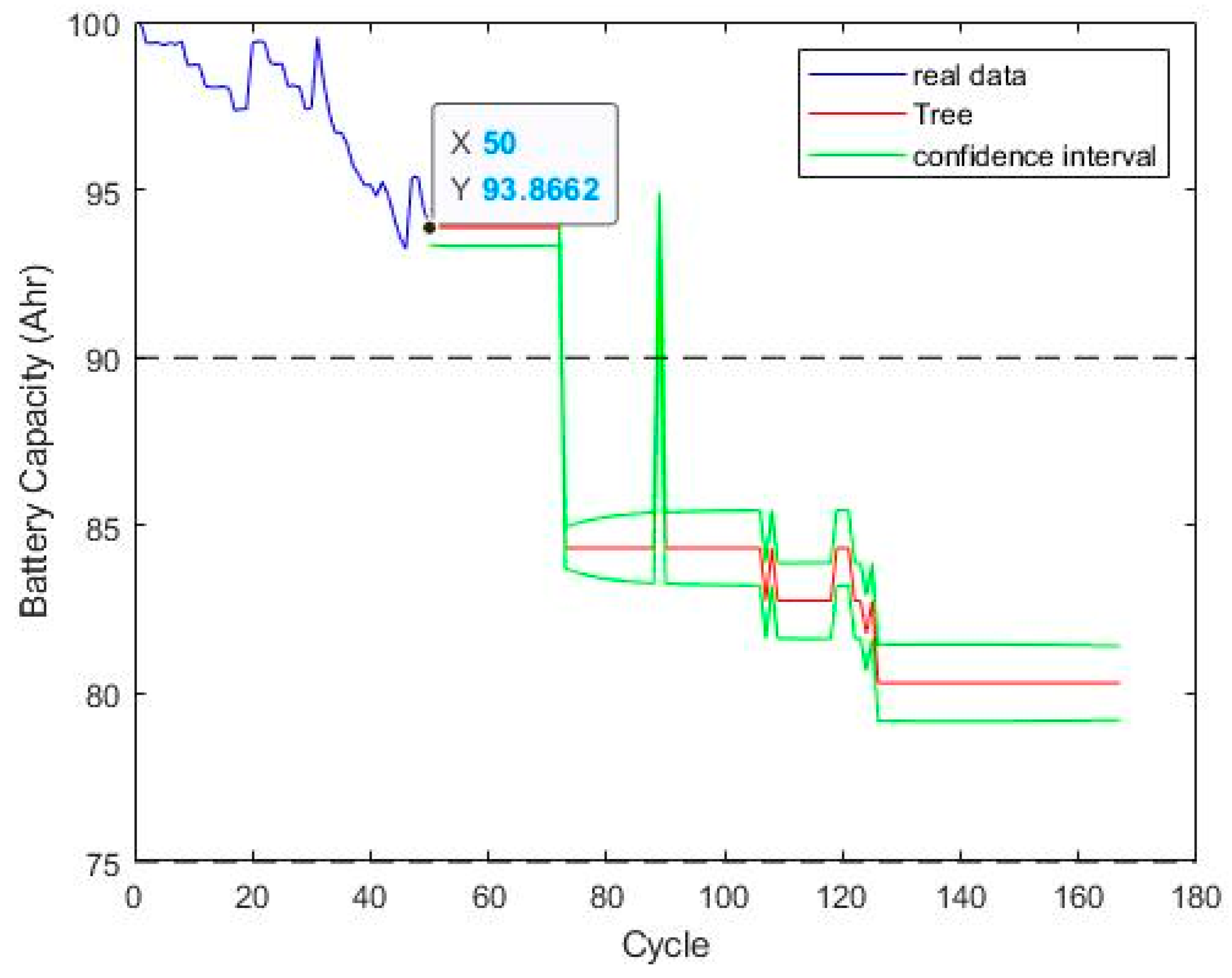
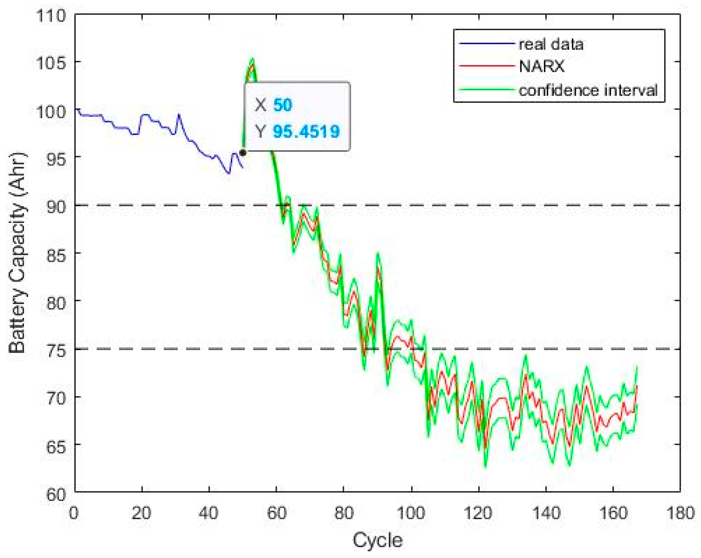
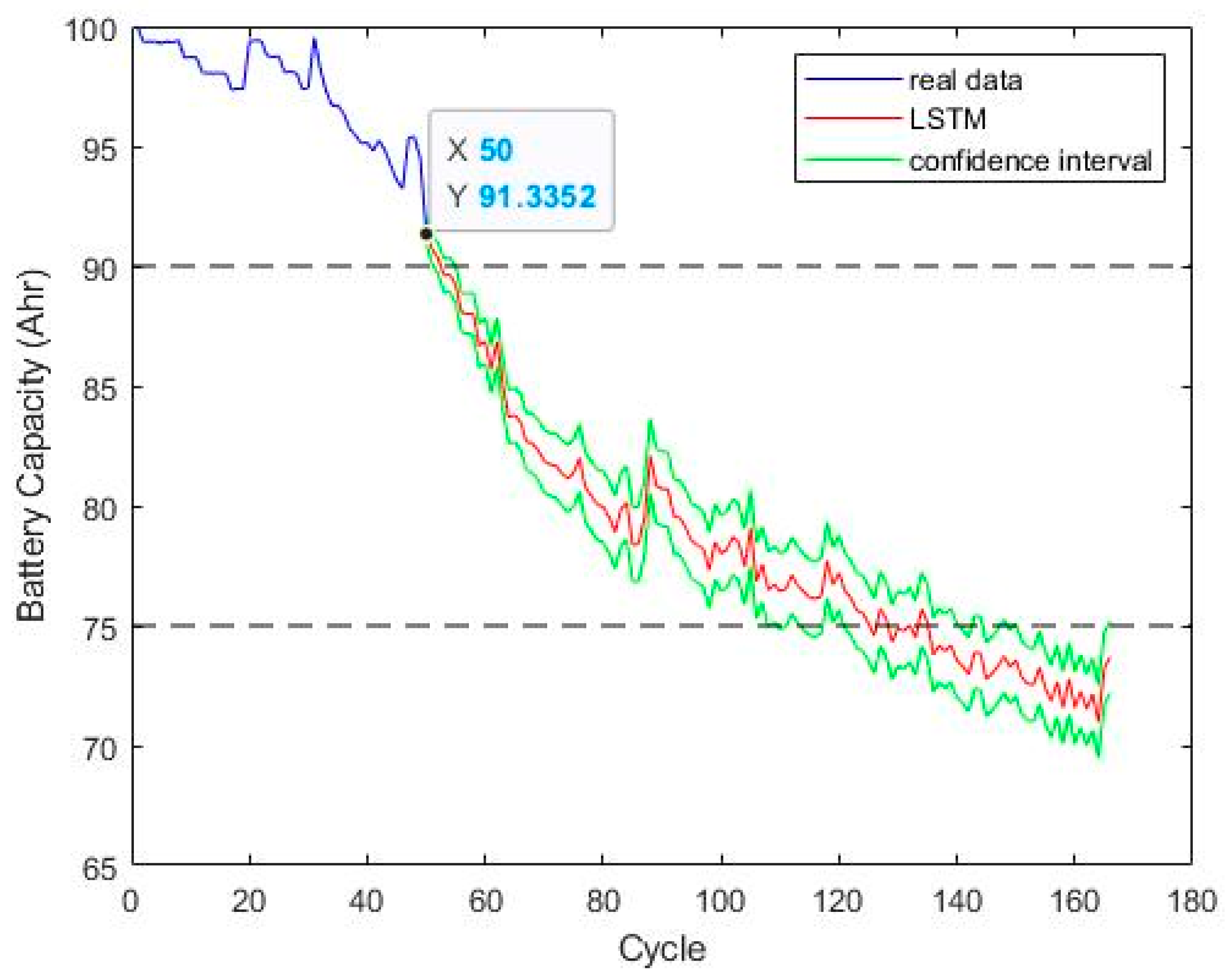
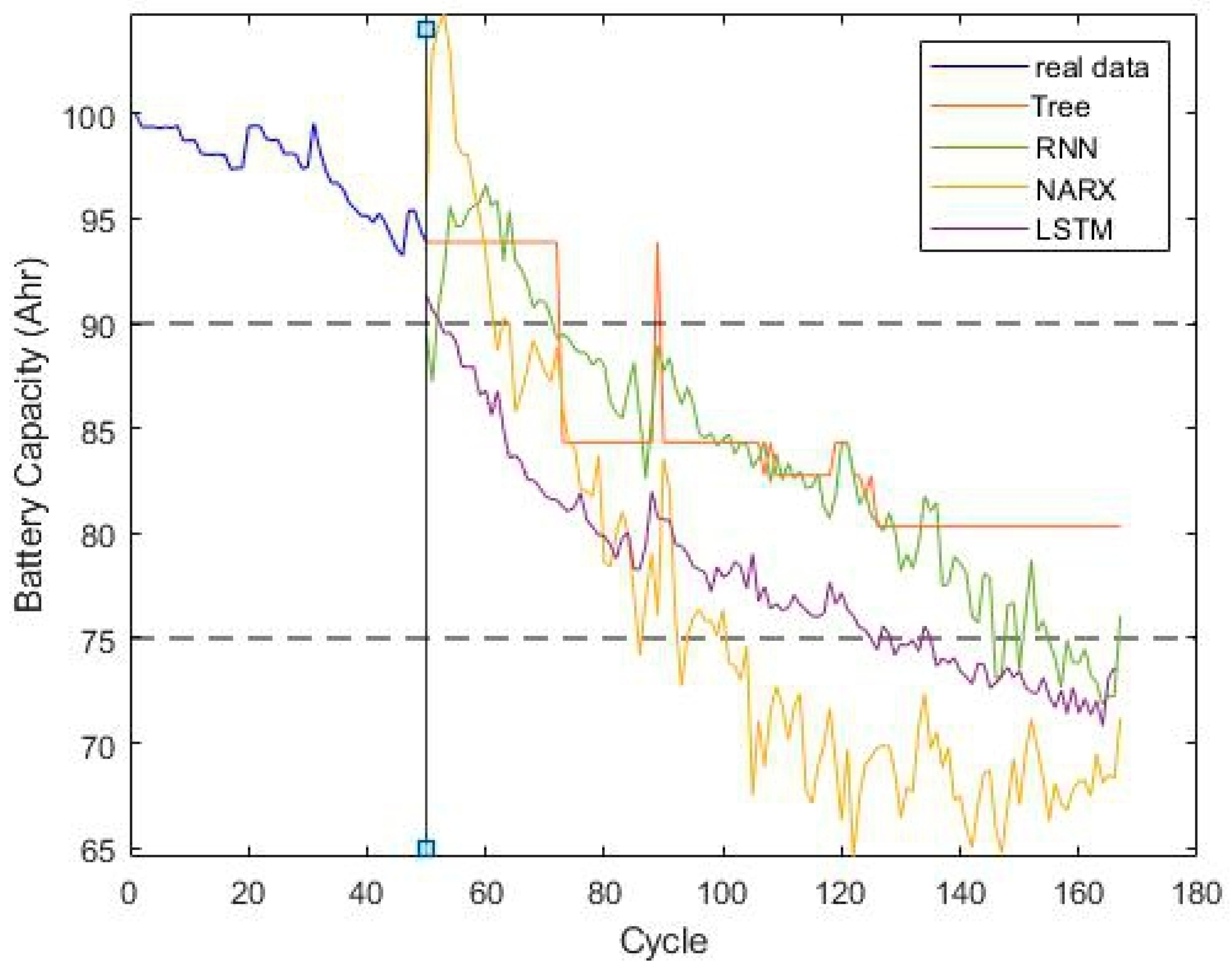
This paper introduces the essential characteristics of lithium-ion batteries and the charging and power measurement methods. In this study, MATLAB is used to design an analysis process to predict the remaining useful life of Li-ion batteries according to NASA’s Li-ion battery aging datasets. The main steps of data processing include data preprocessing, feature extraction, and finding dominant features through correlation analysis. In addition, model training and testing are carried out according to the selected model, and then health indicators and the remaining useful life are generated. During the analysis process, it can be found that the model produced by less data has a large difference between the predicted and actual ones. As the amount of training data increases, the variations in the predicted trends will gradually converge, and the confidence of results will also increase. From the final prediction results, it is known that if the model has a lower loss function, the corresponding remaining life prediction accuracy is higher. After comparative analysis, among the four selected models, the long short-term memory network model has the best prediction effect. The long short-term memory network has the advantage of sharing the characteristics of the recurrent neural network, and adds mechanisms such as the forgetting gate, input gate, and output gate to the hidden layer to discard and update the state to solve the problem of long-term dependence of the recurrent neural network. In this study, the software is successfully used to complete the remaining useful life of Li-ion batteries. In the future, the process developed in this study can be extended to various applications in predictive maintenance.

References

1. Mujib, A.A.; Djatna, T. Ensemble Learning for Predictive Maintenance on Wafer Stick Machine Using IoT Sensor Data. In Proceedings of the 2020 International Conference on Computer Science and Its Application in Agriculture, Bogor, Indonesia, 17 September 2020; pp. 1–5. [Google Scholar]
2. Umeda, S.S.; Tamaki, K.; Sumiya, M.; Kamaji, Y. Planned Maintenance Schedule Update Method for Predictive Maintenance of Semiconductor Plasma Etcher. In Proceedings of the 2020 International Symposium on Semiconductor Manufacturing, Tokyo, Japan, 12–13 December 2020; pp. 1–4. [Google Scholar]
3. Poor, P.; Basl, J.; Zenisek, D. Predictive Maintenance 4.0 as Next Evolution Step in Industrial Maintenance Development. In Proceedings of the 2019 International Research Conference on Smart Computing and Systems Engineering, Colombo, Sri Lanka, 28 March 2019; pp. 245–253. [Google Scholar]
4. Liu, Q.; Hu, Y.; Yu, X.; Qin, Y.; Meng, T.; Hu, X. The Pursuit of Commercial Silicon-based Microparticle Anodes for Advanced Lithium-ion Batteries: A Review. Nano Res. Energy 2022, 1, e9120037. [Google Scholar] [CrossRef]
5. Eshetu, G.G.; Zhang, H.; Judez, X.; Adenusi, H.; Armand, M.; Passerini, S.; Figgemeie, E. Production of High-Energy Li-ion Batteries Comprising Silicon-containing Anodes and Insertion-type Cathodes. Nat. Commun. 2021, 12, 5459. [Google Scholar] [CrossRef] [PubMed]
6. Meng, L.; Wang, G.; See, K.W.; Wang, Y.; Zhang, Y.; Zang, C.; Zhou, R.; Xie, B. Large-Scale Li-Ion Battery Research and Application in Mining Industry. Energies 2022, 15, 3884. [Google Scholar] [CrossRef]
7. Han, X.; Lu, L.; Zheng, Y.; Feng, X.; Li, Z.; Li, J.; Ouyang, M. A review on the key issues of the lithium-ion battery degradation among the whole life cycle. eTransportation 2019, 1, 100005. [Google Scholar] [CrossRef]
8. Gomez, J.; Nelson, R.; Kalu, E.E.; Weatherspoon, M.H.; Zheng, J.P. Equivalent Circuit Model Parameters of a High-power Li-ion Battery: Thermal and State of Charge Effects. J. Power Sources 2011, 196, 4826–4831. [Google Scholar] [CrossRef]
9. Suresh, P.; Shukla, A.K.; Munichandraiah, N. Temperature dependence studies of a.c. impedance of lithium-ion cells. J. Appl. Electrochem. 2002, 32, 267–273. [Google Scholar] [CrossRef]
10. Seo, M.; Song, Y.; Park, S.; Kim, S.W. Capacity Estimation of Lithium-ion Batteries under Various Temperatures using Two Aging Indicators. In Proceedings of the 2021 21st International Conference on Control, Automation and Systems, Jeju, Republic of Korea, 12–15 October 2021; pp. 457–461. [Google Scholar]
11. Lefkowitz, R.J. Identification of adenylate cyclase-coupled betaadrenergic receptors with radiolabeled beta-adrenergic antagonists. Biochem. Pharmacol. 1975, 24, 1651–1658. [Google Scholar] [CrossRef]
12. Zhang, R.; Pan, Z. Model Identification of Lithium-Ion Batteries Considering Current-Rate Effects on battery impedance. In Proceedings of the 2019 4th International Conference on Power and Renewable Energy, Chengdu, China, 21–23 September 2019; pp. 305–309. [Google Scholar]
13. Du, J.; Sun, Y. The Influence of High Power Charging on the Lithium Battery Based on Constant and Pulse Current Charging Strategies. In Proceedings of the 2020 IEEE Vehicle Power and Propulsion Conference, Gijon, Spain, 18 November 2020; pp. 1–7. [Google Scholar]
14. Al Rasyid, A.Z.J.; Firmansyah, E.; Wijaya, F.D. Modeling of Temperature Effect on SoC of Lithium-Ion Battery Pack. In Proceedings of the 2021 3rd International Symposium on Material and Electrical Engineering Conference, Bandung, Indonesia, 10–11 November 2021; pp. 299–303. [Google Scholar]
15. Shen, S.; Liu, B.; Zhang, K.; Ci, S. Toward Fast and Accurate SOH Prediction for Lithium-Ion Batteries. IEEE Trans. Energy Convers. 2021, 36, 2036–2046. [Google Scholar] [CrossRef]
16. Tong, S.; Klein, M.P.; Park, J.W. On-line optimization of battery open circuit voltage for improved state-of-charge and state-of-health estimation. J. Power Sources 2015, 293, 416–428. [Google Scholar] [CrossRef]
17. Islam, S.M.R.; Park, S.-Y. Precise Online Electrochemical Impedance Spectroscopy Strategies for Li-Ion Batteries. IEEE Trans. Ind. Appl. 2020, 56, 1661–1669. [Google Scholar] [CrossRef]
18. Li, Z.; Wu, X.; Guo, B.; Jia, H.; Bai, F. Lithium Battery Health Status Assessment Method Based on Failure Physical Model. In Proceedings of the 2021 IEEE 4th International Conference on Electronics Technology, Chengdu, China, 7–10 May 2021; pp. 394–399. [Google Scholar]
19. Hu, X.; Yuan, H.; Zou, C.; Li, Z.; Zhang, L. Co-Estimation of State of Charge and State of Health for Lithium-Ion Batteries Based on Fractional-Order Calculus. IEEE Trans. Veh. Technol. 2018, 67, 10319–10329. [Google Scholar] [CrossRef]
20. Cacciato, M.; Nobile, G.; Scarcella, G.; Scelba, G. Real-time modelbased estimation of SOC and SOH for energy storage systems. In Proceedings of the 2015 IEEE 6th International Symposium on Power Electronics for Distributed Generation Systems, Aachen, Germany, 22–25 June 2015; pp. 1–8. [Google Scholar]
21. Wu, J.; Wang, Y.; Zhang, X.; Chen, Z. A Novel State of Health Estimation Method of Li-ion Battery using Group Method of Data Handling. J. Power Sources 2016, 327, 457–464. [Google Scholar] [CrossRef]
22. Chaoui, H.; Ibe-Ekeocha, C.C. State of Charge and State of Health Estimation for Lithium Batteries Using Recurrent Neural Networks. IEEE Trans. Veh. Technol. 2017, 66, 8773–8783. [Google Scholar] [CrossRef]
23. Liu, D.; Zhou, J.; Liao, H.; Peng, Y.; Peng, X. A Health Indicator Extraction and Optimization Framework for Lithium-ion Battery Degradation Modeling and Prognostics. IEEE Trans. Syst. Man Cybern. Syst. 2015, 45, 915–928. [Google Scholar]
24. McCall, J.J. Maintenance Policies for Stochastically Failing Equipment: A Survey. Manag. Sci. 1965, 11, 493–524. [Google Scholar] [CrossRef]
25. Shin, J.-H.; Jun, H.-B. On Condition based Maintenance Policy. J. Comput. Des. Eng. 2015, 2, 119–127. [Google Scholar] [CrossRef] [Green Version]
26. Zhang, W.; Yang, D.; Wang, H. Data-Driven Methods for Predictive Maintenance of Industrial Equipment: A Survey. IEEE Syst. J. 2019, 13, 2213–2227. [Google Scholar] [CrossRef]
27. Ahmad, R.; Kamaruddin, S. An Overview of Time-based and Condition-based Maintenance in Industrial Application. Comput. Ind. Eng. 2012, 63, 135–149. [Google Scholar] [CrossRef]
28. Huynh, K.T.; Grall, A.; Berenguer, C. A Parametric Predictive Maintenance Decision-Making Framework Considering Improved System Health Prognosis Precision. IEEE Trans. Reliab. 2019, 68, 375–396. [Google Scholar] [CrossRef] [Green Version]
29. Jardine, A.K.S.; Lin, D.; Banjevic, D. A Review on Machinery Diagnostics and Prognostics Implementing Condition-based Maintenance. Mech. Syst. Signal Process. 2006, 20, 1483–1510. [Google Scholar] [CrossRef]
30. Sanchez-Silva, M.; Frangopol, D.; Padgett, J.; Soliman, M. Maintenance and Operation of Infrastructure Systems: Review. J. Struct. Eng. 2016, 142, F4016004. [Google Scholar] [CrossRef]
31. Xiong, R.; Zhang, Y.; Wang, J.; He, H.; Peng, S.; Pecht, M. LithiumIon Battery Health Prognosis Based on a Real Battery Management System Used in Electric Vehicles. IEEE Trans. Veh. Technol. 2019, 68, 4110–4121. [Google Scholar] [CrossRef]
32. Hu, Z.; Bin, J.; Yin, L.; Chen, X. Predictive maintenance strategy of variable period of power rransformer based on reliability and cost. In Proceedings of the 2013 25th Chinese Control and Decision Conference, Guiyang, China, 25–27 May 2013; pp. 4803–4807. [Google Scholar]
33. Chang, W.-Y. The State of Charge Estimating Methods for Battery: A Review. ISRN Appl. Math. 2013, 2013, 953792. [Google Scholar] [CrossRef] [Green Version]
34. Yu, Z.; Chen, X.; Zhou, Y. The Influence of Coupling of Charge/Discharge Rate and Short Term Cycle on the Battery Capacity of Li-ion Batteries. In Proceedings of the 2019 3rd International Conference on Electronic Information Technology and Computer Engineering, Xiamen, China, 18–20 October 2019; pp. 469–473. [Google Scholar]
35. Fatullah, M.A.; Rahardjo, A.; Husnayain, F. Analysis of Discharge Rate and Ambient Temperature Effects on Lead Acid Battery Capacity. In Proceedings of the 2019 IEEE International Conference on Innovative Research and Development, Jakarta, Indonesia, 28–30 June 2019; pp. 1–5. [Google Scholar]
36. Redondo-Iglesias, E.; Venet, P.; Pelissier, S. Measuring Reversible and Irreversible Capacity Losses on Lithium-Ion Batteries. In Proceedings of the 2016 IEEE Vehicle Power and Propulsion Conference, Hangzhou, China, 17–20 October 2016; pp. 1–5. [Google Scholar]
37. Hasib, S.A.; Islam, S.; Chakrabortty, R.K.; Ryan, M.J.; Saha, D.K.; Ahamed, M.H.; Moyeen, S.I.; Das, S.K.; Ali, M.F.; Islam, M.R.; et al. A Comprehensive Review of Available Battery Datasets, RUL Prediction Approaches, and Advanced Battery Management. IEEE Access 2021, 9, 86166–86193. [Google Scholar] [CrossRef]
38. Audin, P.; Jorge, I.; Mesbahi, T.; Samet, A.; De Beuvron, F.D.B.; Boné, R. Auto-encoder LSTM for Li-ion SOH prediction: A comparative study on various benchmark datasets. In Proceedings of the 2021 20th IEEE International Conference on Machine Learning and Applications, Pasadena, CA, USA, 13–16 December 2021; pp. 1529–1536. [Google Scholar]
39. NASA’s Open Data Portal. Li-Ion Battery Aging Datasets. Available online: https://data.nasa.gov/dataset/Li-ion-Battery-Aging-Datasets/uj5r-zjdb (accessed on 10 October 2021).
40. Dodge, Y. The Oxford Dictionary of Statistical Terms; Oxford University Press Inc.: New York, NY, USA, 2006. [Google Scholar]
41. Hamnett, A.; Vielstich, W. Electrochemistry. Russ. J. Electrochem. 2000, 36, 342–343. [Google Scholar]
42. Lehman, A.; O’Rourke, N.; Hatcher, L.; Stepanski, E. JMP for Basic Univariate and Multivariate Statistics: Methods for Researchers and Social Scientists, 2nd ed.; SAS Institute Inc.: Cary, NC, USA, 2013. [Google Scholar]
43. Udo, W.; Muhammad, Y. Data-Driven Predictive Maintenance of Wind Turbine Based on SCADA Data. IEEE Access 2021, 9, 162370–162388. [Google Scholar] [CrossRef]
44. Li, Y.; Liu, K.; Foley, A.M.; Zülke, A.; Berecibar, M.; Nanini-Maury, E.; Van Mierlo, J.; Hoster, H.E. Data-driven Health Estimation and Lifetime Prediction of Lithium-ion Batteries: A review. Renew. Sustain. Energy Rev. 2019, 113, 109254. [Google Scholar] [CrossRef]
Figure 1. CC and CV charging process.
Energies 16 03096 g001
Figure 2. Framework for the predictive maintenance of Li-ion batteries.
Energies 16 03096 g002
Figure 3. CC-CV charging and discharging process of Li-ion battery.
Energies 16 03096 g003
Figure 4. Capacity of Li-ion batteries.
Energies 16 03096 g004
Figure 5. Feature variations in the charging stage related to cycles.
Energies 16 03096 g005
Figure 6. Feature variations in the discharging stage related to cycles.
Energies 16 03096 g006
Figure 7. Features in the charging stage.
Energies 16 03096 g007
Figure 8. Features in the discharging stage.
Energies 16 03096 g008
Figure 9. Flow of model building.
Energies 16 03096 g009
Figure 10. Prediction trends with different learning models (50% data for model training).
Energies 16 03096 g010
Figure 11. Prediction trends with different learning models (70% data for model training).
Energies 16 03096 g011
Figure 12. Flow of health indicator and remaining useful life.
Energies 16 03096 g012
Figure 13. Prediction results of Decision Tree (after 50 cycles).
Energies 16 03096 g013
Figure 14. Prediction results of NARX (after 50 cycles).
Energies 16 03096 g014
Figure 15. Prediction results of RNN (after 50 cycles).
Energies 16 03096 g015
Figure 16. Prediction results of LSTM (after 50 cycles).
Energies 16 03096 g016
Figure 17. Prediction analysis and remaining useful life with LSTM.
Energies 16 03096 g017
Figure 18. Prediction results of different training models.
Energies 16 03096 g018