Article

Exploring the Driving Factors and Their Spatial Effects on Carbon Emissions in the Building Sector

1
School of Economics and Finance, Xi’an Jiaotong University, Xi’an 710061, China
2
Future City Innovation Technology Co., Ltd., Shaanxi Construction Engineering Holding Group, Xi’an 712000, China
3
SCEGC-XJTU Joint Research Center for Future City Construction and Management Innovation, Xi’an Jiaotong University, Xi’an 712000, China
4
Shaanxi Construction Engineering Group Co., Ltd., Xi’an 710003, China
*
Author to whom correspondence should be addressed.
Energies 2023, 16(7), 3094; https://doi.org/10.3390/en16073094
Submission received: 28 February 2023 / Revised: 19 March 2023 / Accepted: 27 March 2023 / Published: 28 March 2023
(This article belongs to the Section B3: Carbon Emission and Utilization)

Abstract

:
This study measured the lifecycle carbon emissions of buildings in 30 Chinese provinces from 2005 to 2020 and decomposed the drivers of carbon emissions in the materialization stage and operation stage of building, respectively, using the Stochastic Impacts with the Regression on Population, Affluence, and Technology (STIRPAT) model in order to investigate the drivers of carbon emissions and their spatial influence effects in the building sector. The spatial Durbin model (SDM) was used to thoroughly investigate the spatial effects of carbon emissions and their drivers in the building sector under geographic and economic distances. According to the findings, China’s building sector has a high concentration of carbon emissions in the east and a low concentration in the west. There is also a sizable spatial autocorrelation, and the spatial spillover effects in the materialization and operation stages shift in opposite directions. To help the building sector to achieve the carbon peaking and neutrality goals, specific policy recommendations are made based on the study’s findings.

1. Introduction

The Intergovernmental Panel on Climate Change (IPCC) stressed the need for “immediate, rapid and large-scale reductions in greenhouse gas emissions, without which limiting warming to approximately 1.5 °C or perhaps 2 °C may not be achievable” in its 2021 report in response to the threat posed by greenhouse gas emissions [1], underscoring the urgency of tackling climate change. To meet the challenges posed by climate change, there are currently 133 countries and 121 regions with net zero targets [2]. China is the main source of carbon emissions worldwide, and its carbon emissions are expected to peak by 2030 and reach carbon neutrality by 2060 [3].
In 2020, the building sector accounted for 36% of global end-use energy consumption and 37% of energy-related CO2 emissions [4]. The lifecycle carbon emissions of China’s buildings made up 50% of the country’s total carbon emissions in 2019 [5], and the building sector has great potential to reduce its emissions and is considered one of the key targets for controlling global temperature rise [6]. The manufacturing of building materials and buildings’ operation processes both contribute significantly to the building sector’s indirect and implicit carbon emissions [7], and, hence, it is important to take these emissions into account. Urbanization and industrialization have sped up the growth of the building sector’s energy consumption and carbon emissions [8], promoting cross-regional mobility of the population and making the connection between provinces closer. Under the combined effect of various factors, carbon emissions between provinces show a certain spatial correlation [9]. Clarifying the primary sources of carbon emissions and their spatial effects in the building sector is essential for the relevant departments to develop targeted carbon reduction strategies in the building sector, which is important from a practical standpoint and will help the industry reach its carbon peaking and carbon neutrality goals.
In order to analyze the variables that affect carbon emissions, researchers frequently employ index decomposition analysis (IDA) [10], structural decomposition analysis (SDA) [11], Kaya identity [12], IPAT model, and its extended model STIRPAT [13]. In comparison, the Kaya identity can generally only be used for the decomposition of drivers, and the specific utility of each driver cannot be measured [14]. SDA demands extensive and thorough sectoral input–output data, which are frequently challenging to obtain in a timely manner. Based on the IPAT model, which divides the driving factors of environmental performance into three types—population, affluence, and technology—the STIPRPAT considers nonlinear situations, overcomes the limitations of the original model, and allows for more refined analysis, such as determining ecological resilience, conducting falsifiable tests of theories such as the Environmental Kuznets Curve (EKC), and exploring the nonlinear effects of drivers on environmental impacts. Compared with IDA, the STIRPAT model has superior scalability and is more suitable for multidimensional driving factors studies [15], so the STIRPAT model was chosen to analyze the drivers of carbon emissions in the building sector (CEBS).
It is vital to take into account CEBS because China currently lacks government statistics on carbon emissions from the building sector. The process-based methodology and the input–output methodology are two typical approaches used in the lifecycle assessment process [16]. The process-based approach focuses on assessing the inputs and outputs of each process in the lifecycle of the object and enables the detailed dismantling of carbon emissions and the analysis of specific processes [17]. The input–output method uses economic flow to reflect the energy flow process, which needs to use data from the input–output table [18]. However, the input–output table is updated less frequently, while the process method can obtain relevant data through the statistical yearbook, and given data availability and timeliness, this paper adopts the process method to account for building carbon emissions.
Numerous studies on drivers of CEBS focus on specific building types or stages, such as public buildings [14,19], urban buildings [20], construction stages [21], operation stages [22], etc. It lacks a holistic perspective to comprehend the lifecycle of CEBS. There are some differences between the primary driving forces behind carbon emissions in the embodied phase and the operation stage as a result of the various sources of carbon emissions. The construction industry is more closely tied to the materialization stage, whereas the population and the growth of tertiary industries are more closely connected to the operation stage. This study divides the CEBS into the materialization stage and the operation stage in order to clearly understand the driving factors of carbon emissions at each stage of the whole building’s lifecycle.
In addition, most studies do not consider the spatial effect of CEBS or just focus on the differences in carbon emissions between regions, such as using geographically and temporally weighted regression (GTWR) models [23] or the Theil index [24] to measure the regional heterogeneity of drivers, while few studies have decomposed the effect of building carbon emissions drivers on the influence of different regions. Spatial econometric models can effectively identify the direct impacts of drivers and their spatial effects, and they are widely used in research about carbon emissions [25], but their utilization in the field of buildings is not yet extensive enough. The spatial Durbin model (SDM) contains both the spatial terms of the dependent and independent variables and can analyze the spatial spillover effects of the dependent and independent variables simultaneously, providing it with superiority over other spatial econometric models such as the spatial error model (SEM) and spatial autoregressive model (SAR). Therefore, this paper initially selects SDM for the analysis of spatial effects, and it is found that the model that meets the actual situation is derived by the Lagrange multiplier (LM) test and the likelihood ratio (LR) test. In addition, most of the current studies only use a single geographical or economic weight matrix to portray the spatial relationship [26], while, in fact, the proximity of geographical location and economic level may have different influence paths and results on carbon emissions, and it is challenging to fully comprehend the spatial consequences of CEBS with a single spatial weight matrix. So, the effect of different spatial distances is taken into account in this paper.
This study uses the STIRPAT model to dissect the drivers of lifecycle CEBS, which offers a more thorough perspective for the research on the drivers of CEBS to address these research gaps. The structure of this paper is as follows: Section 2 presents research methods and data sources; Section 3 depicts the empirical results; Section 4 presents the analysis and discussion of the results; Section 5 provides the research conclusions and corresponding policy recommendations, as well as the shortcomings of this study and future research prospects.

2. Materials and Methods

2.1. Accounting for CEBS

The overall carbon emissions of a building consist of the emissions caused by the energy used in the four phases of the lifecycle of a building: the manufacturing and transportation of building materials, construction, operation, and demolition. Since the yearbook statistics combine the energy consumption of both construction and demolition, these values are typically included in the calculating procedure. The following is the calculating formula:
C E = C E m a + C E c o n + C E o p
where C E denotes the lifecycle CEBS. The carbon emissions from the manufacture and transportation of building materials, the building’s construction and deconstruction, and its operation are represented, respectively, by C E m a , C E c o n , and C E o p .
The following equation accounts for carbon emissions from the manufacturing and delivery of building materials:
C E m a = i = 1 5 [ M i × E F m a , i × ( 1 ε i ) ] + r = 1 3 i = 1 5 ( q i r × d i r × E F t r , r )
where M i denotes the usage of construction material i —there are five main building materials that are used (steel, cement, glass, wood, and aluminum) based on the available data. E F m a , i and ε i denote the carbon emissions factor and recycling factor of the material i , respectively. Since recycled glass and wood are usually not used in building structures, only the recycling factors of steel and aluminum are considered [27]. Construction materials are mainly transported by means of three modes of transportation—rail, road, and waterways—and q i r denotes the weight of material i transported by the mode of transportation r , which is calculated from the percentage of freight transported by rail, road, and waterways in that year. d i r denotes the average transportation distance of the building material i by the mode of transportation r , and E F t r , r denotes the carbon emissions factor of the mode of transportation r .
Equation (3) illustrates that the direct and indirect carbon emissions from these energy consumptions are the carbon emissions in this stage:
C E c o n = j = 1 n ( E j × E F j ) + E e l × E F e l + E h e × E F h e
where C E c o n denotes the carbon emissions of the construction and demolition stages; E j denotes the energy consumption from fossil energy j ; E F j denotes the carbon emissions factor of the fossil energy j ; E e l and E F e l denote the use of electricity and the carbon emissions factor of electricity, respectively; and E h e and E F h e denote the use of heat and the carbon emissions factor of heat, respectively.
The primary and secondary energy consumption of natural gas, electricity, and heat is where the majority of the carbon emissions from the operation phase of the building come from. In this paper, we referred to the building energy consumption splitting model established by Cai [28] for carbon emissions accounting in the operation stage, as shown in Equation (4):
C E o p = C E s e r + C E o t h + C E r e s C E t r a
where C E s e r denotes the carbon emissions of the “wholesale, retail, accommodation and catering” sector, C E o t h denotes the “other” sector’s carbon emissions, C E r e s denotes the carbon emissions of “residential consumption”, and C E t r a denotes the carbon emissions of transportation consumption from the above three sectors, which is represented by all gasoline and all diesel used in household life, along with 95% of the gasoline and 35% of the diesel used in commercial and public services [29]. The calculation of carbon emissions of individual sectors is based on Equation (3).

2.2. Spatial Weight Matrix

Quantifying geographic locational relationships is the aim of the spatial weight matrix. Different spatial weight matrices reflect different spatial relationships. Considering that the carbon emissions of buildings in each place may be influenced by both the geographical location distribution and the economic development level of each province, the following three spatial weight matrices were considered simultaneously in the subsequent spatial measurement analysis to explore the spatial effects under different distance relationships.
  • The binary contiguity spatial weight matrix (W1) uses the binary form to reflect the geographic proximity, where w i j is 1 if two provinces border each other and 0 otherwise;
  • The geographical distance weight matrix (W2) is measured as:
w i j = { 1 / | d i j | i j 0 i = j
where d i j represents the geographical distance between two provinces calculated using the longitude as well as the latitude of their respective provincial administrative centers;
3.
The economic distance weight matrix (W3) is defined as:
w i j = { 1 / | Q i j | i j 0 i = j
where Q i j denotes the gap between the two provinces’ annual average GDP per capita.
In addition, Moran’s I and its scatter plot are important tools for exploring spatial autocorrelation. Moran’s I may be used to perform a preliminary test of spatial correlation, and the various stages of spatial correlation can be easily seen on Moran’s scatter plot. The global Moran’s I is defined as follows:
M o r a n s   I = n i j w i j × i j w i j ( x i x ¯ ) ( x j x ¯ ) i ( x i x ¯ ) 2
where w i j denotes the spatial weight matrix, x i denotes the observed value of area i , and the significance of the global Moran’s I means that there is a spatial correlation, and a positive value indicates a positive spatial relationship and vice versa.
To further examine the aggregation phenomenon in specific regions, the local Moran’s I can be applied to reveal the spatial aggregation characteristics of independent units. The equation of the local Moran’s I is as follows:
I i = n ( x i x ¯ ) i j w i j ( x j x ¯ ) i ( x i x ¯ ) 2
The local Moran’s I results can be used to generate the Moran’s I scatter plot, which displays the aggregation dispersion between regions.

2.3. Model Settings

Based on the STIRPAT model, this study develops a decomposition model of the drivers of CEBS. The STIRPAT model is obtained by improving on the IPAT model, which is a quantitative relational model for measuring human activities’ effects on the environment. The original STIRPAT model is as follows:
I = a P b A c T d e
where I denotes the environmental impact, and P , A , and T refer to population, affluence, and technology, respectively; a is a constant term, e is the random disturbance term, and b , c , and d are exponents of P , A and T , respectively. Equation (10) is usually written in logarithmic form in the calculation as follows:
I = a + b ln P + c ln A + d ln T + e
Considering that building carbon emissions are spatially correlated, a spatial econometric method is introduced, and a general equation to the specific spatial measurement model is adopted, with the model set as follows:
Y i t = ρ W Y i t + X i t β + θ W X i t + α + μ i + υ t + ε i t
where W is a spatial weight matrix; μ i and υ t denote province individual fixed effects and time fixed effects, respectively; ρ is the explained variable’s spatially lag-added value; and θ denotes the explanatory variables’ spatial correlation coefficient.
The carbon emissions characteristics at every phase of the construction are combined to create the decomposition models for the materialization stage and operation stage, respectively, based on the aforementioned model.

2.3.1. Materialization Stage

Carbon emissions in the building materialization stage mainly originate from the new construction process in that year. Based on the existing literature and the decomposition improvement of the STIRPAT model, the drivers of carbon emissions in the building materialization stage were selected as follows.
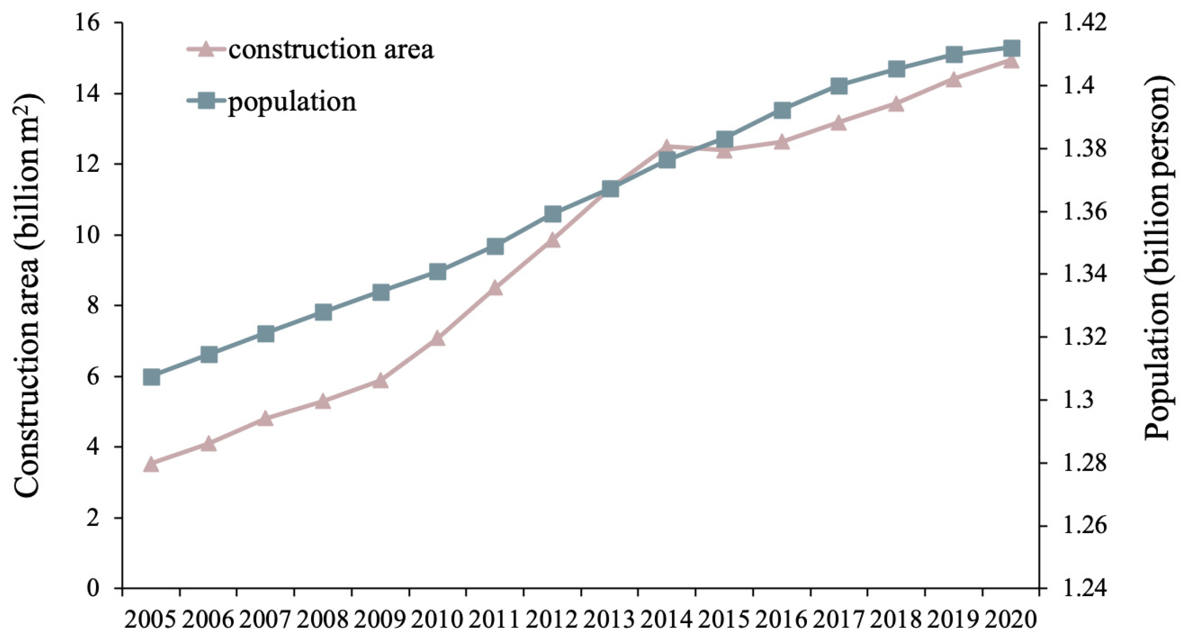
  • Construction area (CA). For the population factor in the model, it is important to consider that the carbon emissions in the annual building materialization stage mainly originate from the new buildings in that year, which could not be measured simply with the population number. Since the building area and population usually show a high correlation [30], the annual new building construction area was chosen to reflect the population factor in the original model;
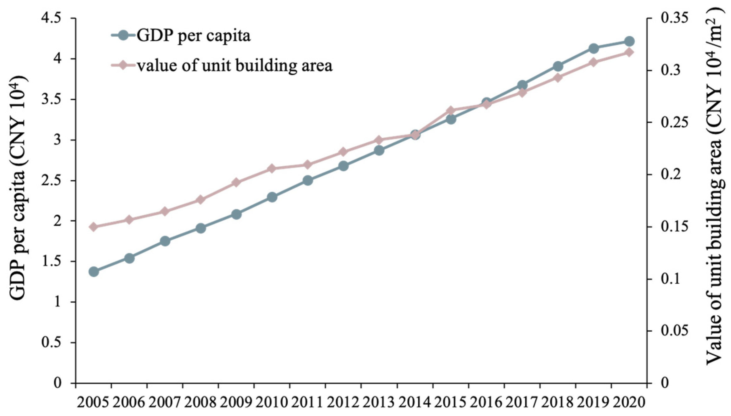
  • Unit completed area value (UV). To correspond to the selection of the population factor indicator above, the unit completed area value was chosen to represent affluence in the materialization stage [31];
  • Labor productivity (LP). Labor productivity in the construction industry can reflect the technological level of the building construction process, but the direction of the impact of the improvement of labor productivity in the building materialization stage remains to be explored. So, this paper selected the performance-based variable construction LP to reflect the technological level of the construction industry;
  • Energy intensity (EI). The energy used during the building construction process is what causes the direct carbon emissions of the materialization stage, and in this case, the energy intensity of the building industry was chosen to reflect the energy used during the materialization stage;
  • Industrial structure (IS). A sizable portion of carbon emissions during the materialization stage come from the production of building materials, which means that the construction industry largely promotes the development of heavy industries such as steel and cement. So, the ratio of the production value of the secondary industry to the total output value served as a measure of the impact of industrial structure on carbon emissions in the materialization stage in this study;
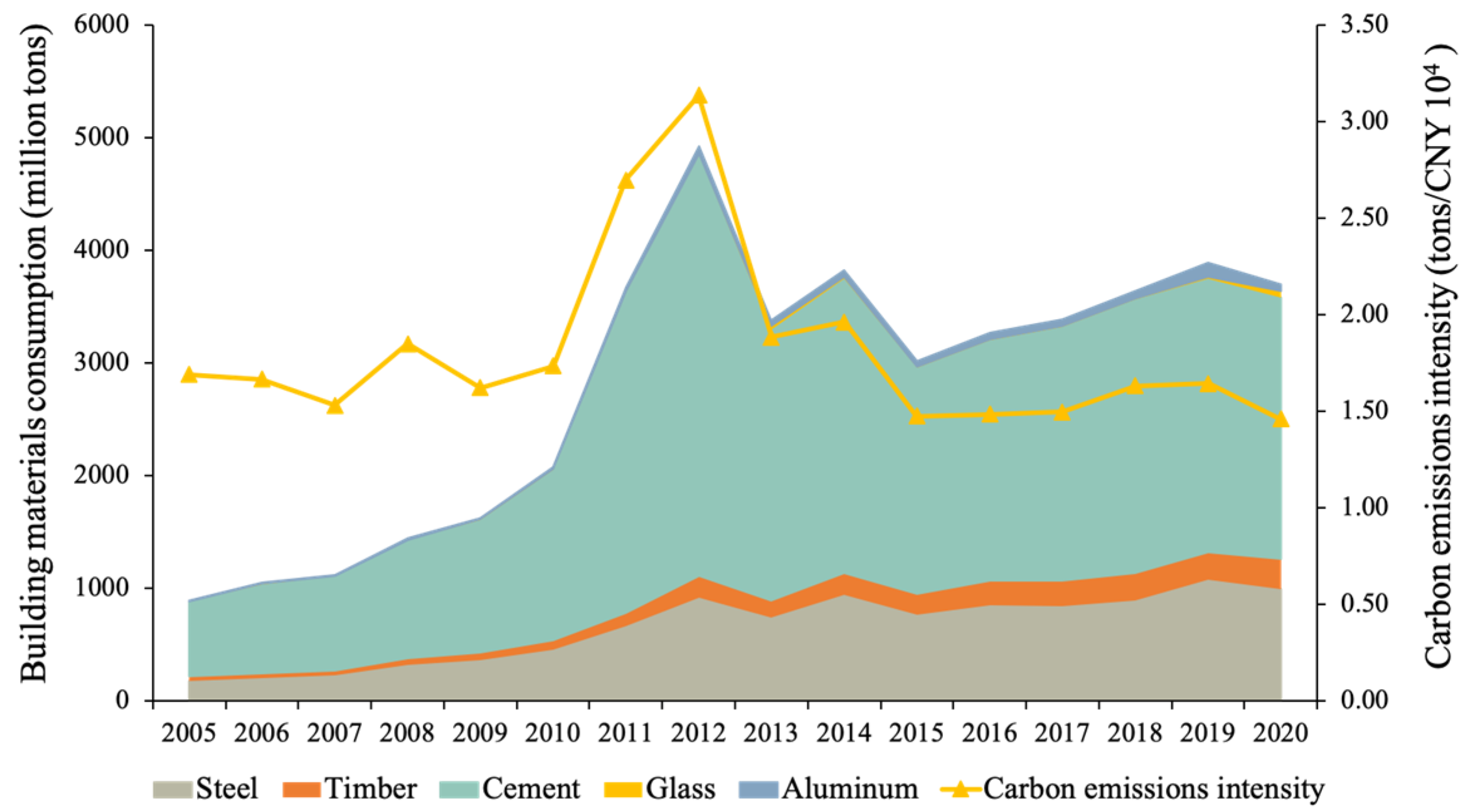
  • Carbon emissions intensity of building materials (MI). The manufacture of building materials generates the majority of indirect carbon emissions during the materialization stage, and these emissions are typically linked to the industrialization process of building material producers. Referring to Zhu [31], the technological elements involved in the manufacture and processing of building materials were measured by the amount of carbon emissions produced by construction materials per unit of production.

2.3.2. Operation Stage

In the building operation stage, existing residential and public buildings are the primary sources of carbon emissions, which is more likely to be impacted by stock considerations than the materialization stage. The following are descriptions of the motivating reasons and metrics.
  • Population (P). Both the daily life and consumption activities of the population contribute to the energy consumption of residential and commercial buildings, so the population size has a significant impact on carbon emissions in the building operation stage;
  • Economic growth (PGDP). The affluence factor is typically quantified by GDP per capita, and the relationship between carbon emissions and economic expansion might not be linear. According to the traditional EKC hypothesis, environmental damage and economic expansion are inversely correlated in a U-shaped pattern. Furthermore, Bruyn [32] argued that the impact of industrial structure and technical development on emissions reduction will gradually wane, and when it cannot offset the environmental pressure caused by economic scale expansion, the Kuznets curve will rise again, showing an N-shaped dynamic trend. Therefore, the higher sub-term of GDP per capita was considered in this study;
  • Level of urbanization (UP and UT). Urbanization drives economic growth and the raising of people’s living standards, which is also usually accompanied by large amounts of carbon emissions [33]. Urbanization causes the growth of the urban population and the prosperity of tertiary industry, which are the main sources of carbon emissions in the operation phase. Therefore, this paper selected the urban population share (UP) and tertiary industry share (UT) as the structural metrics of the urbanization level;
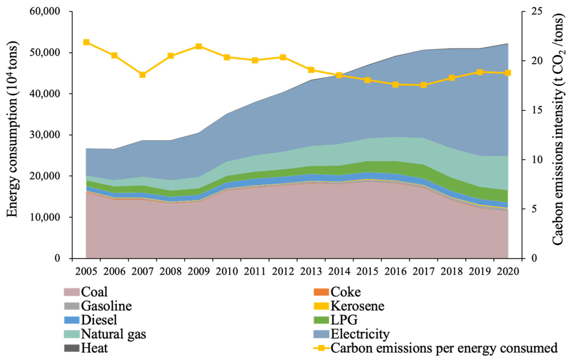
  • Energy consumption (EI, ER, and EC). The principal source of carbon emissions during the building’s operational phase is the use of primary and secondary energy sources such natural gas, electricity, and heat. Energy intensity (EI) and energy structure are the metrics used in this paper to reflect energy use throughout the operational stage. The average carbon emissions intensity (EC) of energy consumption and the proportion of electricity are the major indicators of the energy structure (ER) because electricity is the most promising secondary energy among the main energy sources to achieve low and zero carbon development, and promoting electrification of the operation stage has considerable potential to reduce emissions in the future when clean energy generation technologies are increasingly mature.

2.4. Data Sources

The building materials consumption data in each province were from the China Construction Statistical Yearbook. The China Statistical Yearbook provides data on the volume of freight transported annually with railroads, highways, and canals, and the China Energy Statistical Yearbook provides data on the use of different types of fossil fuels. The General Guidelines for Determining Comprehensive Energy Consumption GB/T 2589-2020 and the China Energy Statistics Yearbook are used to calculate the average low-level heat generation. The unit calorific value carbon content data were obtained from the “Carbon content per unit calorific value of fossil fuels by sector and fuel species” of the provincial inventory, and the carbon oxidation rate is taken from the data published in the 2005 China Greenhouse Gas Study and Carbon Emission Accounts & Datasets (CEADs). Because of the difficulty of splitting the power grids of individual provinces with neighboring provinces, the carbon emissions factor of regional power grids was used in this paper to calculate the carbon emissions of purchased electricity, and the data were obtained from the Average Carbon Dioxide Emissions Factor of China’s Regional Power Grids in 2011 and 2012 published by the National Development and Reform Commission.
The descriptions of the driving factors are shown in Table 1.

3. Results

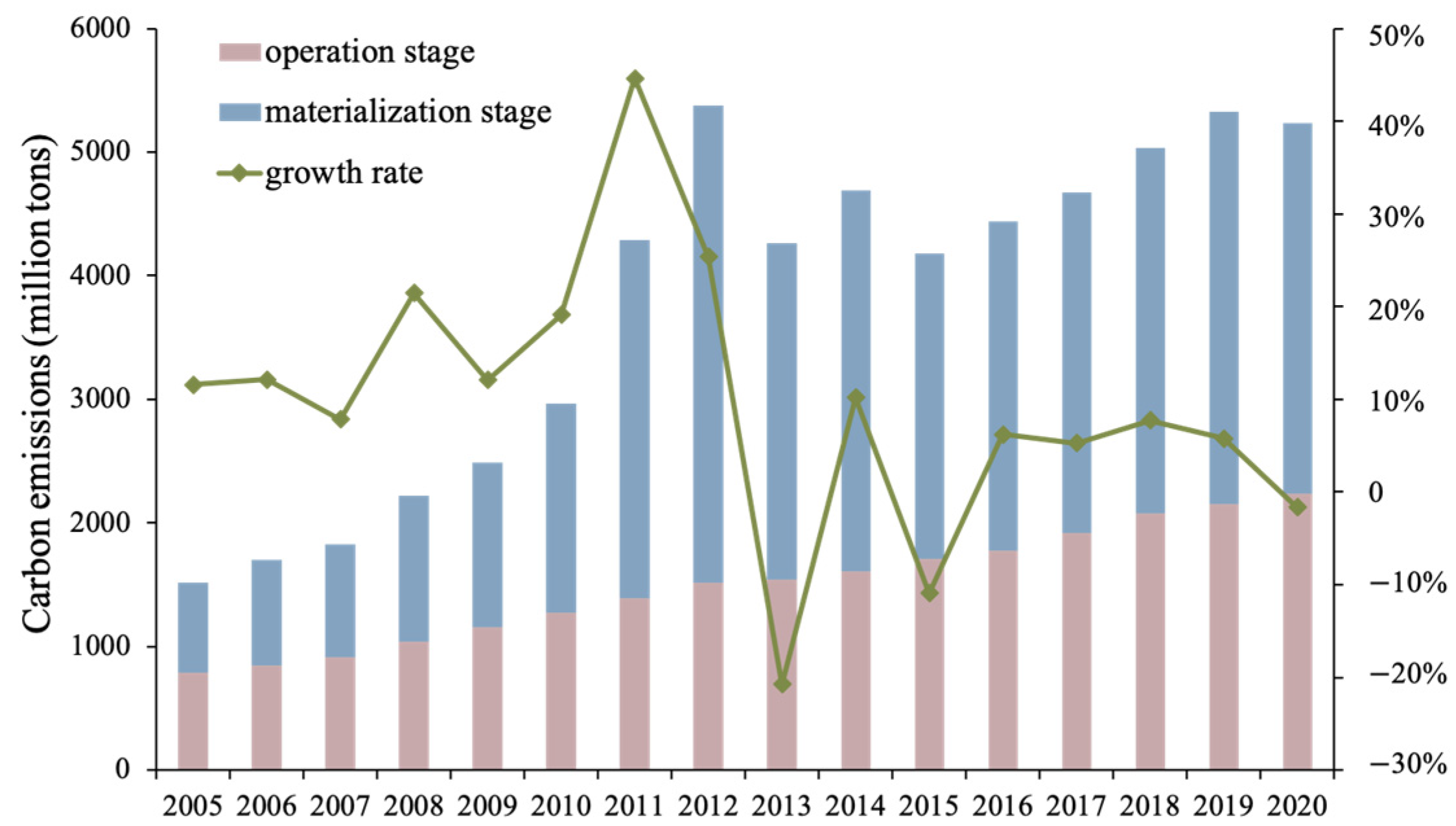
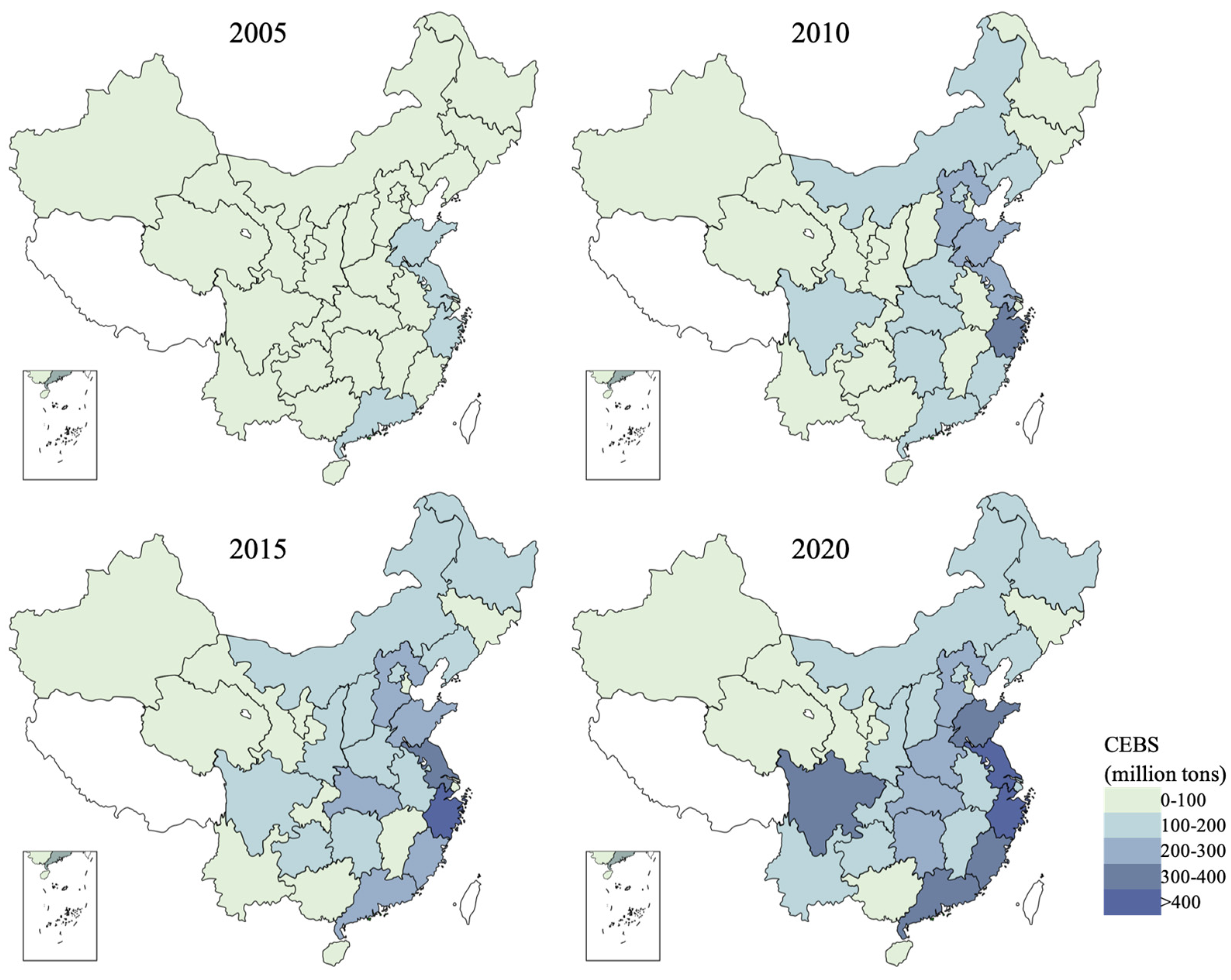
3.1. CEBS from 2005 to 2020

Since there are missing data for some provinces, this paper selected the data from 30 provinces from 2005 to 2020 for carbon emissions accounting, and the results are shown in Figure 1. China’s CEBS in 2020 is 5.238 billion tons, 3.46 times that in 2005. The overall trend of CEBS is on the rise, maintaining an annual growth rate of about 15% until 2009, with a faster growth rate and large fluctuations from 2010 to 2014. This abnormal fluctuation mainly exists in the materialization stage, and it cannot be excluded that there is a problem with the statistical caliber of building materials in the yearbook data [34]. The growth rate from 2015 to 2020 gradually becomes smaller, reaching less than 10%. It is noteworthy that, except for the abnormal fluctuation from 2010 to 2014, the CEBS in 2020 decreased for the first time.
Figure 2 reflects the spatial distribution of CEBS in 2005, 2010, 2015, and 2020. With a gradual increase from the west to the east, the building sector’s carbon emissions in the eastern coastal area are typically greater than those in the western region, and the difference in carbon emissions between regions has further expanded over time. The provinces with the highest building carbon emissions in 2020 are Jiangsu (443.73 million tons) and Zhejiang (438.98 million tons), while the provinces with the lowest building carbon emissions are Hainan (16.13 million tons), Qinghai (17.48 million tons), and Ningxia (17.89 million tons), with large differences between provinces. In terms of growth rate, the provinces with the highest growth rates of building carbon emissions from 2005 to 2020 were Fujian, Jiangxi, and Sichuan, with growth rates of 615.16%, 563.16%, and 464.85%, respectively.

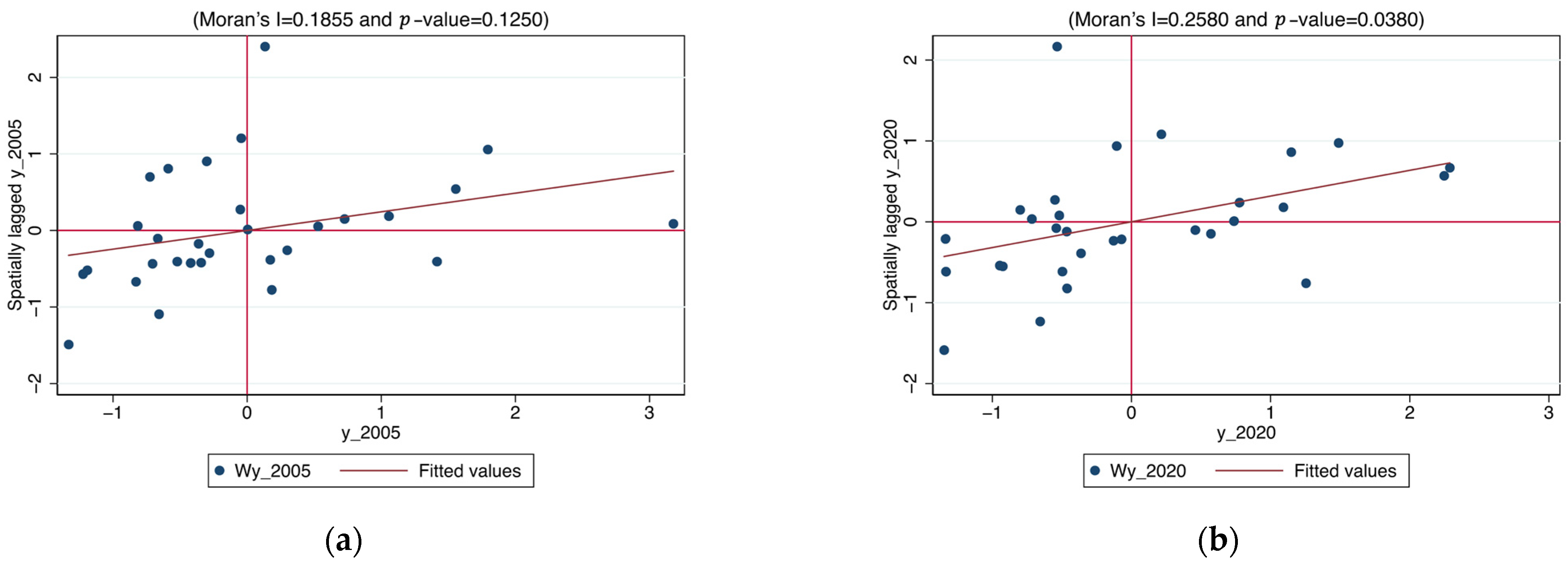
3.2. Spatial Correlation Test

The global Moran’s I test was performed for the CEBS from 2005 to 2020 using W1, W2, and W3, respectively, and Table 2 displays the final outcomes. The spatial distribution of carbon emissions in the Chinese building industry is not fully random and clearly exhibits a positive spatial correlation, as shown by the global Moran’s I of CEBS under various spatial weight matrices, being positive in all cases and passing the significance test in most instances—i.e., provinces with high carbon emissions tend to be spatially adjacent—and there is a certain spatial spillover effect which needs to be taken into consideration. Moran’s I under W3 has a low significance among them, demonstrating that the spatial spillover impact of CEBS is more a function of the surrounding area. In addition, except for the anomalous years of 2010–2014, the overall Moran’s I shows an increasing trend, indicating that the spatial effect of CEBS is gradually increasing.
To further investigate the spatial association among provinces, the Moran’s I scatter plot was calculated and drawn based on the adjacency matrix using the local Moran’s I. Due to space limitations, only Moran’s I scatter plots for 2005 and 2020 are shown here in Figure 3. The first and third quadrants of the figure include the majority of the corresponding points, showing that the majority of the provinces are either of the high–high (H–H) or low–low (L–L) aggregation type. This is in line with the global Moran’s I test findings.

3.3. Selection of Spatial Econometric Models

Some tests, such as the Lagrange multiplier test (LM test), likelihood ratio test (LR test), and Hausman test, can be used to examine the spatial effects of carbon emissions in the materialization and operation stages and to choose an appropriate spatial econometric model. The aforementioned tests were conducted for the carbon emissions models in the materialization stage and operational stage using three different spatial weight matrices, and the outcomes are displayed in Table 3. Significant terms are found in all of the LM tests using various spatial weight matrices, demonstrating the necessity of using a spatial econometric model for the analysis. The SDM model is chosen for the regression, since the LR test indicates that it should not degenerate into the SEM or SAR model. It should be decided based on a fixed-effects model, according to the Hausman results.

3.4. Regression Results

3.4.1. Stationary Test

Panel data need to be tested for stationarity before regression to avoid spurious regression. To explore whether a variable is a stationary time series, a unit root test is usually performed on it, and the Im, Pesaran, and Shin (IPS) test was chosen to test the unit root, since this paper uses short panel data. Since the initial test found unit roots in the variables, the IPS test was performed after taking the first-order difference for all variables to determine whether cointegration analysis could be performed. Table 4 reflects the results of the test after first-order difference, and it can be seen that the first-order difference of all variables passed the unit root test, which means that all variables are integrated of order one.
To verify whether there is a common stochastic trend in multiple unit root series, the Pedroni test was selected for cointegration analysis. Table 5 reflects the Pedroni cointegration test results for the variables in the materialization stage and operation stage, and the panel data all passed the cointegration test, allowing for subsequent analysis.

3.4.2. Results of the Materialization Stage

The SDM model’s regression findings for the materialization stage are shown in Table 6. In a spatial econometric model with a spatial lag term, the regression coefficient alone could not express the connection between the independent and dependent variables [35]. LeSage and Pace [36] separated the effect into three categories: the direct effect, indirect effect, and total effect, which represent the direct effect of the independent variable on the dependent variable in the region, the indirect effect on the dependent variable in neighboring regions, and their overall effect, respectively. Hence, Table 6 solely displays the outcomes of direct, indirect, and cumulative effects.
Under various spatial weights, the direct effect coefficients almost always point in the same direction, demonstrating the robustness of the regression findings. Local carbon emissions have a significant promoting effect on local carbon emissions in the materialization stage and a significant radiating pulling effect on neighboring areas’ carbon emissions. Although the value of the unit building space promotes local carbon emissions, the impact on the neighborhood is adverse, and the inhibiting effect on the surrounding areas is less than the promoting effect on the local area. The impact of construction labor productivity varies under different spatial matrix conditions, with a relatively weak promoting effect on local carbon emissions in the materialization stage and a suppressing effect on regions with similar levels of economic development. The direction of energy intensity’s influence in the materialization stage is significantly positive, but the effect is not as strong as it might be due to the fact that the intensity of direct energy consumption corresponds to the carbon emissions in the construction and demolition stage, whereas these emissions are much lower in the materialization stage and are primarily caused by indirect carbon emissions. Therefore, it is easier to see how construction materials’ carbon emissions intensity affects local carbon emissions during the materialization stage while also having a minor moderating effect on emissions in nearby locations. In the materialization stage, the growth of the secondary industry significantly contributes to local carbon emissions and has more pronounced spillover effects in areas with comparable economic development. Due to competition between construction businesses in nearby regions, the spatial coefficient of carbon emissions at the materialization stage is notably negative.

3.4.3. Results of the Operation Stage

The SDM model’s regression findings for the operating stage are shown in Table 7. Each driver has a sizable direct impact on the region’s carbon emissions at the operational stage, and the effects persist under various spatial matrices with some robustness.
The population contributes significantly to carbon emissions during operation, exerts the most direct influence, and has a slight radiation pull effect on emissions during operation in nearby areas. The operational stage of the connection between economic growth and carbon emissions is represented by an N-shaped curve. Specifically, early economic growth will cause a sharp rise in carbon emissions during the operational period, and at a later stage, due to increased environmental protection awareness and advancements in technology, there is a certain suppression effect on carbon emissions, followed by a rebound trend. Similar impacts on carbon emissions are caused by economic development in nearby areas during the operational phase. The degree of urbanization significantly promotes the region’s operational carbon emissions., and there is no evidence of the inverted U-shaped influence curve that has been described in some studies. The growth of tertiary industry likewise raises carbon emissions during operation, although it has a dampening effect on emissions during operation in the neighborhood. In terms of energy consumption, both energy intensity and average energy carbon intensity have a significant contribution to operational carbon emissions, while increasing the share of electricity in energy end consumption helps to reduce operational stage carbon emissions. Energy-type influencing factors typically do not have strong enough geographic effects, and, hence, they are not discussed. The spatial coefficients of carbon emissions in the operational stage are notably positive, suggesting that there is a spatial spillover effect and a positive impact effect of reciprocal promotion between surrounding areas and provinces with similar economic development levels.

4. Discussion

4.1. Population-Based Driving Factors

Population-based drivers (CA and P) significantly boost CEBS as well as those in surrounding provinces due to spatial spillover effects. This is consistent with Chen [22] and Wu [37]. The growth in population size creates a demand for housing and public services, which contributes to the growth in the number of houses and the operational energy consumption of residential and public buildings. Typically, there is more frequent population movement between adjacent provinces. These movements alter the population stock, altering the demand for floor space and raises carbon emissions in adjacent provinces. Figure 4 reflects the changes in population and building construction area in China from 2005 to 2020, showing that the construction area and population have changed in the same direction, both showing an upward trend, but the growth rate has slowed down. In addition to satisfying people’s living needs, real estate also has a certain financial nature [38], which makes the change in building construction area and population number not fully consistent and may lead to excessive building area expansion.

4.2. Affluence-Based Driving Factors

The affluence-based drivers VA and PGDP both contribute to CEBS, where GDP per capita has an N-shaped curve on carbon emissions in the operation stage, which is the same as in the findings of Fakher [39] and Allard [40]. The value of a unit building area can reflect people’s requirements for the quality, functionality, and aesthetics of construction projects [31], and as people’s living standards and income levels increase, they are no longer satisfied with the general residential nature of houses and have higher requirements for their quality, workmanship, and appearance. The increased consumption of building supplies and labor causes the output value per finished area to climb steadily (as depicted in Figure 5), which raises carbon emissions during the materialization stage. The GDP per capita is likewise continuously increasing. The holdings of all types of electrical equipment dramatically expand as people’s living conditions significantly improve during the early stages of economic development, which has a large pulling effect on carbon emissions during the operational stage. However, as the economy grows to a certain point, low-carbon technology advancement, environmental legislation, and increased environmental protection consciousness all work to slow the growth of carbon emissions in the operating stage. With the optimization of structure and technology, the marginal effect of progress gradually decreases, and when its growth cannot cover the increment of operational carbon emissions brought by the expansion of economic scale, economic growth can no longer be decoupled from the operation stage carbon emissions but again shows a promoting effect.

4.3. Technology-Based Driving Factors

4.3.1. Urbanization and Industrial Structure

Urbanization greatly contributes to carbon emissions in the operating stage of buildings, and the quadratic term’s coefficient is also highly positive, suggesting that as urbanization and economic development continue, so will their effect on these emissions, which verifies the findings of Huo [30] for carbon emissions in public buildings. Urbanization is usually accompanied by economic growth and an increase in residents’ income level, and its influence path on carbon emissions in the operation stage is similar to that of affluence-based drivers, but there is no inflection point effect yet, which may be due to the fact that the existing urbanization level has not yet met the demands of the rural–urban migration population. The urbanization rate in developed countries is generally above 80% at present [41], while the only provinces in China with an urbanization rate above 80% in 2020 were Beijing, Tianjin, and Shanghai, and the urbanization rate in some provinces is just above 50%. Therefore, for the time being, the effect of urbanization on carbon emissions is still being promoted positively. The rise in tertiary output value is also one of the signs of urbanization, and it has also promoted carbon emissions in the operation stage of the region. The tertiary industry is represented by the carbon emissions of public buildings, which in 2020 represented 42% of total emissions during the operation stage and were the highest among all categories of civil buildings. As a result, an increase in the tertiary industry’s share will drive an increase in carbon emissions in the operation stage, which is similar to the findings of Xiao [42] on carbon emissions from urban buildings. The siphoning effect may be to blame for the fact that the growth of the tertiary industry has a certain inhibitory effect on the carbon emissions in the operational stage of the surrounding areas [43]. Since competition exists between cities in geographical proximity, the distribution of resources of high-quality service industries may be skewed toward the central city, which is detrimental to the development of the tertiary industry in the surrounding areas. Secondary industry contains the construction and building materials’ manufacturing industries, and the increase in its output value share will promote carbon emissions. Secondary industry also has a certain siphoning effect in neighboring areas, but there is a positive spatial spillover effect among regions with similar economic development, which may be explained by the different optimal choices of industrial structure in cities at different stages of development. Therefore, the industrial development paths of cities with similar economies are similar, and there is a mutual promotion effect.

4.3.2. Energy Intensity and Structure

As a direct source of carbon emissions, energy intensity contributes significantly to CEBS. Its spatial spillover effect is not robust, and the positive spillover effect is more obvious under the adjacency matrix. It is favorable to reduce carbon emissions at the building operation stage by increasing the share of electricity in end-use energy consumption, which is in line with the findings of Liu [19]. Because increasing the amount of power produced from renewable sources can lower the intensity of carbon emissions, the average carbon emissions factor of the grid in China has decreased from 0.6101 tCO2/MWh in 2015 to 0.5703 tCO2/MWh in 2022, meaning that China is likely to achieve zero carbon emissions in the future [44]. Moreover, the average carbon emissions intensity of total energy consumption can partially represent the structure of energy use. The percentage of energy with a high carbon emissions factor increases with an increase in the average carbon emissions intensity of energy. The main energy usage in the building sector changed between 2005 and 2020, as shown in Figure 6. This statistic only accounts for the energy used during the structure’s construction, demolition, and operating phases because it is challenging to measure the energy used during the creation of building components. These days, the three main energy sources employed in the building sector are electricity, coal, and natural gas. Compared with 2005, the consumption and share of coal have decreased, the consumption and share of electricity have increased significantly, and the consumption of natural gas and LPG have also increased, while the overall change in other energy sources is not significant. The average carbon emissions intensity of energy decreased compared to 2005, but rebounded after 2017, indicating that the energy consumption structure of the building sector needs to be further optimized.

4.3.3. Labor Productivity in the Construction Industry

The impact of labor productivity on CEBS is a topic of some debate among academics. Li [25] argued that the rise in worker productivity in the construction sector indicates that the sector is advancing energy-saving technology, embracing technological innovation, and modernizing, while Zhang [45] argued that higher labor productivity means higher output value can be created per unit of labor, and this process is usually accompanied by higher carbon emissions, so labor productivity in the construction sector reduces carbon emissions in the sector. The regression results in 3.4 demonstrate that, whereas labor productivity in the building industry significantly inhibits emissions in locations with similar levels of economic growth, it adds positively to carbon emissions in the region’s materialization stage. This may be because an increase in labor productivity leads to an increase in the region’s construction output, which in turn results in higher carbon emissions. Meanwhile, due to the competition effect, construction enterprises in other provinces with similar development will improve their competitiveness through technological innovation and other means, and, thus, the suppression phenomenon occurs. It can be seen that the decomposition results with the spatial effects can explain the controversial phenomena in the literature and are more accurate in representing the actual situation.

4.3.4. Carbon Emissions Intensity of Building Materials

The strongest pulling force on local carbon emissions occurs at the materialization stage due to the carbon emissions intensity of construction materials, which is consistent with Zhu [31]. More than half of lifecycle CEBS are linked to building materials [46]. Carbon emissions from building materials are primarily affected by the preparation process and the consumption structure, and this article focuses primarily on the latter. Figure 7 illustrates how the consumption pattern of building materials can be inferred from the carbon emissions intensity of these materials. Cement, as the world’s third largest artificial carbon emissions source [47], has a changing share that is basically consistent with the trend of carbon emissions intensity of building materials. Additionally, cement has a non-recyclable nature, unlike steel and aluminum, which can reduce the carbon emissions of the production process by increasing the recycling ratio [44], so the use of cement needs to be controlled to reduce the carbon emissions intensity of building materials. At present, the proportion of cement in China has decreased from 74.19% in 2005 to 62.81% in 2020, which means that the consumption structure of building materials has been optimized to some extent. The carbon emissions intensity of construction materials has a suppressive influence on the materialization stage of carbon emissions in the nearby bordering areas, similar to the spatial effect of the value of the unit building area. Due to the market segmentation effect, administrative boundaries and local protectionism have an impact on the value of unit building area as well as the structure of building materials consumption, which both measure the technical proficiency of regional design and construction firms. Thus, it appears to have a negative effect on the neighborhood.

5. Conclusions

This study divided the causes of CEBS into two categories using the STIRPAT model—the materialization stage and the operation stage—and determined the drivers of ten aspects, such as population, construction area, GDP per capita, the value of unit building area, urbanization rate, industrial structure, energy intensity, energy structure, the labor productivity of the construction industry, and the carbon emissions intensity of building materials, allowing us to test and discuss the possible non-linear effects of factors such as GDP per capita and urbanization rate. By combining the SDM model to decompose the spatial effects of carbon emissions and their drivers in the building sector, the following conclusions were obtained.
  • Except for the abnormal fluctuations from 2010 to 2014, China’s building sector has seen an increase in carbon emissions, which peaked in 2019 and then started to decline in 2020. Each province’s carbon emissions from the building industry exhibit an uneven distribution tendency, gradually increasing from the west to the east, and the gap between areas is widening over time.
  • All of the drivers of CEBS, except for the level of electrification, have a significant positive contribution to carbon emissions in the region. Among them, the effect of GDP per capita shows a rising N-shaped curve, which verifies the N-shaped environmental Kuznets curve hypothesis. The carbon emissions intensity of building materials, construction area, and value of unit building area are the factors that have the biggest impacts on carbon emissions in the region’s materialization stage, while population, GDP per capita, and energy carbon emissions intensity have the biggest impacts on carbon emissions in the operational stage.
  • There is a positive spatial autocorrelation of CEBS. As far as the spatial effect of carbon emissions in each province is concerned, there is a negative effect of carbon emissions in the materialization stage on carbon emissions in the neighboring areas, which is manifested in the crowding-out effect of drivers such as the value of unit building area and the structure of consumption of building materials on the neighboring areas. Due to the influence of demographic factors, the construction area has a positive spatial spillover effect among neighboring regions, and for regions with similar economic development levels, they mainly influence each other through labor productivity and the industrial structure. There is a positive pulling effect of carbon emissions in the operation stage on the neighboring regions, mainly because of the radiation effect of population and economic development on the neighboring regions, but due to the existence of the siphoning effect, the amount of tertiary industry will negatively affect the carbon emissions from operations in nearby areas.
This paper gives the following policy recommendations in response to the above analysis.
  • Controlling the scale of construction. Currently, the rate of change in the building construction sector far exceeds the rate of population growth. Housing speculation can be combated through taxation and purchase restrictions to curb the blind expansion of the construction scale in order to reduce carbon emissions in the materialization phase.
  • Establishing a complete building life-cycle carbon footprint regulatory system. The materialization stage of building materials contributes large amounts of carbon emissions, and it is necessary to establish a full lifecycle carbon footprint regulation system to promote low-carbon technology innovation by upstream building materials enterprises. This can encourage or urge construction enterprises to choose green and low-carbon building materials through subsidies or carbon emissions limit regulations, reduce the proportion of high-carbon emissions building materials such as cement, actively develop and promote wood structures and assembled steel structures, and increase the proportion of recycled metal materials such as steel.
  • Promoting low-carbon and energy-saving lifestyles and optimizing the internal structure of industries. Population growth and urbanization processes are unavoidable. They can change residents’ lifestyles, optimize consumption structures, and promote energy-saving behaviors by increasing education and publicity, advocating low-carbon lifestyles. At the same time, the scale of urban development needs to be controlled to avoid the inefficiency and higher carbon emissions brought about by blind expansion. At the same time, investment in low-carbon industries needs to be strengthened in order to play its leading role in industrial restructuring.
  • Increasing the percentage of clean energy while adjusting the structure of energy use. The building sector should optimize its energy consumption patterns, cut back on the usage of energy with high carbon emissions, and boost the proportion of clean energy to decrease carbon emissions at the source. Governments should increase investment in technical research and the industrial development of clean energy generation technologies such as wind, hydro, solar PV, biomass, etc.
  • Reducing regional administrative barriers and promoting coordinated regional development. The empirical results show that there may be a certain market segmentation effect in the construction industry, which is not conducive to the exchange and dissemination of advanced low-carbon, energy-saving technologies. Therefore, it is essential to lower regional administrative obstacles, maximize human resource use, encourage resource and technology movement across provincial boundaries, and build a network of synergistic sharing mechanisms to promote inter-regional synergistic carbon reduction development.
The drawback of this study is that it used the regional grid carbon emission factors from 2012, which have a time lag and do not accurately reflect the dynamic changes in the electricity carbon emission factors. Therefore, it is difficult to see how the increase in the share of electricity changes the intensity of energy carbon emissions. In addition, this study used a static spatial panel model, which cannot reflect the dynamic changes in the time dimension. Dynamic spatial panel models and multi-perspective decomposition of CEBS can be taken into account in future studies.

Author Contributions

Conceptualization, J.W.; methodology, J.R.; software, J.R.; validation, J.W., J.R.; formal analysis, J.R.; investigation, J.R. and J.P.; resources, J.W. and W.S.; data curation, J.R.; writing—original draft preparation, J.W., J.L. and J.R.; writing—review and editing, J.W., J.R., J.L. and K.W.; visualization, J.R. and J.P.; supervision, J.W.; project administration, J.W. and W.S.; funding acquisition, J.W. and W.S. All authors have read and agreed to the published version of the manuscript.

Funding

This research was financially funded by the SCEGC-XJTU Joint Research Center for Future City Construction and Management Innovation Foundation (SKH2021284).

Data Availability Statement

Not applicable.

Conflicts of Interest

The authors declare no conflict of interest.

Nomenclature

The nomenclature of used abbreviations in this article are explained as follows.
AbbreviationsFull Name
CEBSCarbon Emissions in the Building Sector
IPCCIntergovernmental Panel on Climate Change
IPATthe model for Environmental Impacts of Population, Affluence, and Technology
STIRPATStochastic Impacts by Regression on Population, Affluence, and Technology
IDAIndex Decomposition Analysis
SDAStructural Decomposition Analysis
GTWRGeographically and Temporally Weighted Regression
CEADsCarbon Emission Accounts & Datasets
EKCEnvironmental Kuznets Curve
LM testthe Lagrange Multiplier test
LR testthe Likelihood Ratio test
IPSThe Im, Pesaran, and Shin test
SDMSpatial Durbin Model
SEMSpatial Error Model
SARSpatial Autoregressive Model

References

  1. IPCC. Climate Change 2021: The Physical Science Basis. Available online: https://www.ipcc.ch/report/sixth-assessment-report-working-group-i/ (accessed on 1 January 2023).
  2. MSCI. Net Zero Tracker. Available online: https://zerotracker.net/ (accessed on 3 January 2023).
  3. XINHUANET. Xi Jinping Delivers an Important Speech at the General Debate of the 75th UN General Assembly. Available online: http://www.xinhuanet.com/world/2020-09/22/c_1126527647.htm (accessed on 3 January 2023).
  4. UNEP. 2021 Global Status Report for Buildings and Construction. Available online: https://www.unep.org/resources/report/2021-global-status-report-buildings-and-construction (accessed on 1 January 2023).
  5. CABEE. 2022 Research Report of China Building Energy Consumption and Carbon Emissions. Available online: https://mp.weixin.qq.com/s/7Hr__rkhS70owqTbYI_XuA (accessed on 3 January 2023).
  6. IEA&UNEP. Global Status Report for Buildings and Construction 2019: Towards a Zero-Emissions, Efficient and Resilient Buildings and Construction Sector. Available online: https://www.iea.org/reports/global-status-report-for-buildings-and-construction-2019 (accessed on 3 January 2023).
  7. Zhang, Y.; Yan, D.; Hu, S.; Guo, S. Modelling of energy consumption and carbon emission from the building construction sector in China, a process-based LCA approach. Energy Policy 2019, 134, 110949. [Google Scholar] [CrossRef]
  8. Hong, J.; Liu, Y.; Chen, Y. A spatiotemporal analysis of carbon lock-in effect in China’s provincial construction industry. Resour. Sci. 2022, 44, 1388–1404. [Google Scholar]
  9. Huo, T.; Cao, R.; Xia, N.; Hu, X.; Cai, W.; Liu, B. Spatial correlation network structure of China’s building carbon emissions and its driving factors: A social network analysis method. J. Environ. Manag. 2022, 320, 115808. [Google Scholar] [CrossRef] [PubMed]
  10. Mai, L.; Ran, Q.; Wu, H. A LMDI decomposition analysis of carbon dioxide emissions from the electric power sector in Northwest China. Nat. Resour. Model. 2020, 33, e12284. [Google Scholar] [CrossRef]
  11. Wang, C.; Wang, F.; Zhang, X.; Wang, Y.; Su, Y.; Ye, Y.; Wu, Q.; Zhang, H.O. Dynamic features and driving mechanism of coal consumption for Guangdong province in China. J. Geogr. Sci. 2022, 32, 401–420. [Google Scholar] [CrossRef]
  12. Bigerna, S.; Polinori, P. Convergence of KAYA components in the European Union toward the 2050 decarbonization target. J. Clean. Prod. 2022, 366, 132950. [Google Scholar] [CrossRef]
  13. Li, Z.; Murshed, M.; Yan, P. Driving force analysis and prediction of ecological footprint in urban agglomeration based on extended STIRPAT model and shared socioeconomic pathways (SSPs). J. Clean. Prod. 2023, 383, 135424. [Google Scholar] [CrossRef]
  14. Ma, M.; Yan, R.; Cai, W. An extended STIRPAT model-based methodology for evaluating the driving forces affecting carbon emissions in existing public building sector: Evidence from China in 2000–2015. Nat. Hazards 2017, 89, 741–756. [Google Scholar] [CrossRef]
  15. Yu, S.; Zhang, Q.; Li Hao, J.; Ma, W.; Sun, Y.; Wang, X.; Song, Y. Development of an extended STIRPAT model to assess the driving factors of household carbon dioxide emissions in China. J. Environ. Manag. 2023, 325, 116502. [Google Scholar] [CrossRef]
  16. Saynajoki, A.; Heinonen, J.; Junnila, S.; Horvath, A. Can life-cycle assessment produce reliable policy guidelines in the building sector? Environ. Res. Lett. 2017, 12, 013001. [Google Scholar] [CrossRef] [Green Version]
  17. Liu, G.; Gu, T.; Xu, P.; Hong, J.; Shrestha, A.; Martek, I. A production line-based carbon emission assessment model for prefabricated components in China. J. Clean. Prod. 2019, 209, 30–39. [Google Scholar] [CrossRef]
  18. Liu, J.; Liu, Y.; Yang, L.; Hu, Y. Study on the Calculation Method of Carbon Emission from the Whole Building Industry Chain in China. Urban Stud. 2017, 24, c28–c32. [Google Scholar]
  19. Liu, L.-Q.; Liu, K.-L.; Zhang, T.; Mao, K.; Lin, C.-Q.; Gao, Y.-F.; Xie, B.-C. Spatial characteristics and factors that influence the environmental efficiency of public buildings in China. J. Clean. Prod. 2021, 322, 128842. [Google Scholar] [CrossRef]
  20. Huo, T.F.; Li, X.H.; Cai, W.G.; Zuo, J.; Jia, F.Y.; Wei, H.F. Exploring the impact of urbanization on urban building carbon emissions in China: Evidence from a provincial panel data model. Sust. Cities Soc. 2020, 56, 102068. [Google Scholar] [CrossRef]
  21. Zhang, J.; Li, H.; Xia, B.; Skitmore, M. Impact of environment regulation on the efficiency of regional construction industry: A 3-stage Data Envelopment Analysis (DEA). J. Clean. Prod. 2018, 200, 770–780. [Google Scholar] [CrossRef]
  22. Chen, C.; Bi, L. Study on spatio-temporal changes and driving factors of carbon emissions at the building operation stage- A case study of China. Build. Environ. 2022, 219, 109147. [Google Scholar] [CrossRef]
  23. Du, Z.; Liu, Y.; Zhang, Z. Spatiotemporal Analysis of Influencing Factors of Carbon Emission in Public Buildings in China. Buildings 2022, 12, 424. [Google Scholar] [CrossRef]
  24. Gan, L.; Liu, Y.; Shi, Q.; Cai, W.; Ren, H. Regional inequality in the carbon emission intensity of public buildings in China. Build. Environ. 2022, 225, 109657. [Google Scholar] [CrossRef]
  25. Li, B.; Han, S.; Wang, Y.; Li, J.; Wang, Y. Feasibility assessment of the carbon emissions peak in China’s construction industry: Factor decomposition and peak forecast. Sci. Total Environ. 2020, 706, 135716. [Google Scholar] [CrossRef] [PubMed]
  26. Wang, Y.; He, X. Spatial economic dependency in the Environmental Kuznets Curve of carbon dioxide: The case of China. J. Clean. Prod. 2019, 218, 498–510. [Google Scholar] [CrossRef]
  27. Chen, W.; Yang, S.; Zhang, X.; Jordan, N.D.; Huang, J. Embodied energy and carbon emissions of building materials in China. Build. Environ. 2022, 207, 108434. [Google Scholar] [CrossRef]
  28. Cai, W.; Li, X.; Wang, X.; Chen, M. Split model and application of building energy consumption based on energy balance table. J. HVAC 2017, 47, 27–34. [Google Scholar]
  29. Wang, Q. Study on the statistics and calculation of building energy consumption in China. Energy Conserv. Environ. Prot. 2007, 8, 9–10. [Google Scholar]
  30. Huo, T.; Ren, H.; Cai, W. Estimating urban residential building-related energy consumption and energy intensity in China based on improved building stock turnover model. Sci. Total Environ. 2019, 650, 427–437. [Google Scholar] [CrossRef]
  31. Zhu, C.; Chang, Y.; Li, X.; Shan, M. Factors influencing embodied carbon emissions of China’s building sector: An analysis based on extended STIRPAT modeling. Energy Build. 2022, 255, 111607. [Google Scholar] [CrossRef]
  32. de Bruyn, S.M.; van den Bergh, J.; Opschoor, J.B. Economic growth and emissions: Reconsidering the empirical basis of environmental Kuznets curves. Ecol. Econ. 1998, 25, 161–175. [Google Scholar] [CrossRef]
  33. Huo, T.; Cao, R.; Du, H.; Zhang, J.; Cai, W.; Liu, B. Nonlinear influence of urbanization on China’s urban residential building carbon emissions: New evidence from panel threshold model. Sci. Total Environ. 2021, 772, 145058. [Google Scholar] [CrossRef]
  34. CABEE. China Building Energy Consumption Annual Report 2020. J. BEE 2021, 49, 1–6. [Google Scholar] [CrossRef]
  35. Bai, J.; Wang, Y.; Jiang, F.; Li, J. R&D Element Flow, Spatial Knowledge Spillovers and Economic Growth. Econ. Res. J. 2017, 52, 109–123. [Google Scholar]
  36. Lesage, J.P.; Pace, R.K. Spatial econometric modeling of origin-destination Flows. J. Reg. Sci. 2008, 48, 941–967. [Google Scholar] [CrossRef]
  37. Wu, P.; Song, Y.; Zhu, J.; Chang, R. Analyzing the influence factors of the carbon emissions from China’s building and construction industry from 2000 to 2015. J. Clean. Prod. 2019, 221, 552–566. [Google Scholar] [CrossRef]
  38. Guo, J.; Chen, L.; Gao, G.; Guo, S.; Li, X. Simulation Model-Based Research on the Technology Support System for China’s Real Estate Financial Risk Management. Sustainability 2022, 14, 13525. [Google Scholar] [CrossRef]
  39. Fakher, H.A.; Ahmed, Z.; Acheampong, A.O.; Nathaniel, S.P. Renewable energy, nonrenewable energy, and environmental quality nexus: An investigation of the N-shaped Environmental Kuznets Curve based on six environmental indicators. Energy 2023, 263, 125660. [Google Scholar] [CrossRef]
  40. Allard, A.; Takman, J.; Uddin, G.S.; Ahmed, A. The N-shaped environmental Kuznets curve: An empirical evaluation using a panel quantile regression approach. Environ. Sci. Pollut. Res. 2018, 25, 5848–5861. [Google Scholar] [CrossRef] [PubMed] [Green Version]
  41. Yu, Y.; Yang, B. The Synergy of Urbanization and Structural Upgrading in China. Econ. Perspect. 2021, 10, 3–18. [Google Scholar]
  42. Xiao, Y.; Huang, H.; Qian, X.; Zhang, L.; An, B. Can new-type urbanization reduce urban building carbon emissions? New evidence from China. Sust. Cities Soc. 2023, 90, 104410. [Google Scholar] [CrossRef]
  43. Ye, X.; Long, Y.; Mao, Z. Spatial Pattern and Driving Factors of Multi-level Consumer Cities: A Case Study of 41 Cities in the Yangtze River Delta. Econ. Geogr. 2022, 42, 75–85. [Google Scholar]
  44. Zhang, Y.; Hu, S.; Guo, F.; Mastrucci, A.; Zhang, S.; Yang, Z.; Yan, D. Assessing the potential of decarbonizing China’s building construction by 2060 and synergy with industry sector. J. Clean. Prod. 2022, 359, 132086. [Google Scholar] [CrossRef]
  45. Zhang, S.; Huo, Z.; Zhai, C. Building Carbon Emission Scenario Prediction Using STIRPAT and GA-BP Neural Network Model. Sustainability 2022, 14, 9369. [Google Scholar] [CrossRef]
  46. Luo, Z.; Cang, Y.; Zhang, N.; Yang, L.; Liu, J. A Quantitative Process-Based Inventory Study on Material Embodied Carbon Emissions of Residential, Office, and Commercial Buildings in China. J. Therm. Sci. 2019, 28, 1236–1251. [Google Scholar] [CrossRef]
  47. Andrew, R.M. Global CO2 emissions from cement production, 1928–2017. Earth Syst. Sci. Data 2018, 10, 2213–2239. [Google Scholar] [CrossRef] [Green Version]
Figure 1. China’s CEBS from 2005 to 2020.
Energies 16 03094 g001
Figure 2. Distribution of the CEBS.
Energies 16 03094 g002
Figure 3. Moran’s I scatter plots for 2005 and 2020, (a) Moran’s I scatter plots for 2005; (b) Moran’s I scatter plots for 2020. The first and third quadrants indicate that high-observed-value areas are surrounded by high-observed-value areas (H–H) and low-value areas are surrounded by low-value areas (L–L), respectively, and the second and fourth quadrants indicate that low-value areas are surrounded by high-value areas (L–H) and high-value areas are surrounded by low-value areas (H–L), respectively.
Energies 16 03094 g003
Figure 4. Population and construction area in China from 2005 to 2020.
Energies 16 03094 g004
Figure 5. GDP per capita and value of unit building area in China from 2005 to 2020.
Energies 16 03094 g005
Figure 6. Energy consumption and its carbon emissions intensity in the building sector; the different types of energy consumption are converted to standard coal.
Energies 16 03094 g006
Figure 7. Consumption of building materials and its carbon emissions intensity in the building sector.
Energies 16 03094 g007
Table 1. Descriptions of the driving factors.
SymbolVariableDefinitionUnit
CECarbon emissionsLifecycle CEBSMillion tons
CABuilding construction areaBuilding construction area at the end of the yearMillion m2
PPopulationThe number of residents at the end of the year104 people
UVValue of unit building areaThe proportion of a building’s completed value to its completed areaCNY 104/m2
PGDPGDP per capitaThe ratio of GDP to the populationCNY 104
LPLabor productivityThe ratio of total output value to employees in the construction industryCNY 104/person
EIEnergy intensityDirect energy consumption to added value ratioPJ/CNY 108
ISIndustry structureThe proportion of secondary industry output to overall output%
MICarbon emissions intensity of building materialsThe ratio of carbon emissions from building materials to the construction industry outputTons/CNY 104
UPThe proportion of the urban populationThe proportion of urban residents to all people%
UTThe proportion of the tertiary industryThe proportion of the tertiary industry to total output%
ERLevel of electrificationThe ratio of the electricity consumption to total energy consumption%
ECCarbon emissions intensity of energy consumptionCarbon emissions from direct energy consumption per unitTons/tons
Table 2. Global Moran’s I under different spatial matrices.
YearW1W2W3
20050.152 **0.052 ***0.071
20060.156 **0.052 ***0.063
20070.158 **0.059 ***0.121 *
20080.171 **0.055 ***0.136 *
20090.169 **0.063 ***0.134 *
20100.115 *0.042 **0.113
20110.0620.007 *0.025
2012−0.030−0.022−0.112
20130.0610.030 **0.102
20140.0560.027 **0.066
20150.160 **0.064 ***0.125 *
20160.146 **0.066 ***0.089
20170.199 **0.079 ***0.135 *
20180.203 **0.080 ***0.126 *
20190.283 ***0.095 ***0.130 *
20200.235 ***0.080 ***0.136 *
Note: *** p < 0.01, ** p < 0.05, * p < 0.1.
Table 3. The results of tests.
TestsMaterialization StageOperation Stage
W1W2W3W1W2W3
LM-err0.758
(0.38)
2.549
(0.11)
7.769 ***
(0.005)
42.796 ***
(0.00)
94.399 ***
(0.00)
60.814 ***
(0.00)
LM-lag24.142 ***
(0.00)
3.808 *
(0.05)
1.121
(0.29)
27.481 ***
(0.00)
115.578 ***
(0.00)
4.553 **
(0.03)
LR testSDM
(0.00)
SDM
(0.00)
SDM
(0.00)
SDM
(0.00)
SDM
(0.00)
SDM
(0.00)
Hausman23.61 **
(0.034)
125.47 ***
(0.00)
25.63 **
(0.019)
104.30 **
(0.00)
39.13 ***
(0.001)
50.34 ***
(0.001)
Note: *** p < 0.01, ** p < 0.05, * p < 0.1, p-values in parentheses, LM test results are selected for robustness.
Table 4. IPS test results after 1st difference.
VariablesIPS TestVariablesIPS Test
PanelPanel and TrendPanelPanel and Trend
d.lnCE(M)−10.910 ***
(0.00)
−10.859 ***
(0.00)
d.lnCE(O)−9.385 ***
(0.00)
−9.402 ***
(0.00)
d.lnCA−6.637 ***
(0.00)
−6.403 ***
(0.00)
d.lnP−3.030 ***
(0.00)
−5.733 ***
(0.00)
d.lnUV−10.932 ***
(0.00)
−10.628 ***
(0.00)
d.lnPGDP−3.540 ***
(0.00)
−4.806 ***
(0.00)
d.lnLP−10.598 ***
(0.00)
−8.919 ***
(0.00)
d.lnUP−6.970 ***
(0.00)
−8.200 ***
(0.00)
d.lnEI−10.44 ***−10.709 ***d.lnUT−6.631 ***−6.777 ***
(0.00)(0.00) (0.00)(0.00)
d.lnIS−6.739 ***−7.773 ***d.lnER−9.120 ***−9.650 ***
(0.00)(0.00) (0.00)(0.00)
d.lnMI−11.465 ***−11.191 ***d.lnEI−8.832 ***−9.495 ***
(0.00)(0.00) (0.00)(0.00)
d.lnEC−9.524 ***−9.718 ***
(0.00)(0.00)
Note: *** p < 0.01, p-values in parentheses. lnCE(M) denotes carbon emissions in the materialization stage; lnCE(O) denotes carbon emissions in the operation stage.
Table 5. Pedroni cointegration test results.
Materialization StageOperation Stage
Modified Phillips–Perron t8.246 ***
(0.00)
9.297 ***
(0.00)
Phillips–Perron t−8.893 ***
(0.00)
−15.785 ***
(0.00)
Augmented Dickey–Fuller t−7.804 ***
(0.00)
−7.673 ***
(0.00)
Note: *** p < 0.01, p-values in parentheses.
Table 6. Spatial panel regression results of the materialization stage.
VariablesDirect EffectIndirect EffectTotal Effect
W1W2W3W1W2W3W1W2W3
lnCA0.810 ***0.831 ***0.803 ***0.213 ***0.539 ***−0.0041.022 ***1.369 ***0.798 ***
(0.00)(0.00)(0.00)(0.00)(0.00)(0.93)(0.00)(0.00)(0.00)
lnUV0.519 ***0.522 ***0.504 ***−0.224 ***−0.344 *−0.162 *0.295 ***0.1780.341 ***
(0.00)(0.00)(0.00)(0.01)(0.09)(0.08)(0.01)(0.37)(0.00)
lnLP0.090 **0.0450.075 *−0.052−0.205−0.201 ***0.038−0.16−0.126 *
(0.01)(0.23)(0.05)(0.30)(0.10)(0.00)(0.48)(0.19)(0.05)
lnEI0.065 ***0.059 ***0.076 ***0.091 ***0.0640.0310.156 ***0.122 *0.108 ***
(0.00)(0.00)(0.00)(0.00)(0.36)(0.33)(0.00)(0.09)(0.00)
lnIS0.464 ***0.487 ***0.490 ***−0.262 **−0.2670.754 ***0.202 **0.221.244 ***
(0.00)(0.00)(0.00)(0.02)(0.38)(0.00)(0.11)(0.48)(0.00)
lnMI0.933 ***0.931 ***0.932 ***−0.059 **−0.139 **−0.0290.874 ***0.792 **0.903 ***
(0.00)(0.00)(0.00)(0.03)(0.05)(0.39)(0.00)(0.00)(0.39)
Spatial ρ −0.180 **−1.009 ***−0.233 ***
(0.04)(0.00)(0.00)
LR testbothbothboth
R20.9050.9670.929
Log-L439.27448.22438.88
Note: *** p < 0.01, ** p < 0.05, * p < 0.1, p-values in parentheses.
Table 7. Spatial panel regression results of the operation stage.
VariablesDirect EffectIndirect EffectTotal Effect
W1W2W3W1W2W3W1W2W3
lnP1.623 ***1.567 ***1.511 ***0.297 **−0.0350.363 **1.920 ***1.532 **1.874 ***
(0.00)(0.00)(0.00)(0.03)(0.95)(0.04)(0.00)(0.01)(0.00)
lnPGDP1.338 ***1.308 ***1.282 ***0.0770.671 ***0.449 ***1.414 ***1.979 ***1.731 ***
(0.00)(0.00)(0.00)(0.35)(0.01)(0.00)(0.00)(0.00)(0.00)
lnPGDP2−0.229 ***−0.234 ***−0.178 ***−0.003−0.348 *−0.192 **−0.232 ***−0.582 *−0.370 ***
(0.00)(0.00)(0.00)(0.97)(0.06)(0.04)(0.00)(0.00)(0.00)
lnPGDP30.042 ***0.048 ***0.040 ***0.0050.121 *0.060 *0.047 **0.169 **0.100 ***
(0.00)(0.00)(0.00)(0.79)(0.06)(0.05)(0.04)(0.01)(0.00)
lnUP0.686 ***0.538 ***0.389 ***0.5962.668 *−0.4531.282 *3.206 **−0.064
(0.00)(0.00)(0.01)(0.28)(0.06)(0.44)(0.05)(0.03)(0.92)
lnUP20.354 ***0.267 ***0.178 **0.3262.163 ***0.2210.680 *2.429 ***0.400
(0.00)(0.00)(0.03)(0.28)(0.01)(0.48)(0.06)(0.00)(0.23)
lnUT0.617 ***0.670 ***0.658 ***−0.225 ***−0.531 **0.0230.392 ***0.1390.681 ***
(0.00)(0.00)(0.00)(0.00)(0.02)(0.82)(0.00)(0.55)(0.00)
lnER−0.082 ***−0.104 ***−0.080 ***0.247 ***0.3620.0490.165 *0.258−0.031
(0.00)(0.00)(0.00)(0.00)(0.27)(0.63)(0.08)(0.45)(0.78)
lnEI0.862 ***0.864 ***0.890 ***0.0490.0170.0970.911 ***0.880 ***0.987 ***
(0.00)(0.00)(0.00)(0.30)(0.92)(0.23)(0.00)(0.00)(0.00)
lnEC1.030 ***1.053 ***1.084 ***−0.457−1.5570.480 *0.572−0.5041.565 ***
(0.00)(0.00)(0.00)(0.13)(0.16)(0.06)(0.10)(0.66)(0.00)
Spatial ρ 0.355 ***0.499 ***0.406 ***
(0.00)(0.00)(0.00)
LR testindindind
R20.7610.9230.924
Log-L952.04957.71956.29
Note: *** p < 0.01, ** p < 0.05, * p < 0.1, p-values in parentheses.
Disclaimer/Publisher’s Note: The statements, opinions and data contained in all publications are solely those of the individual author(s) and contributor(s) and not of MDPI and/or the editor(s). MDPI and/or the editor(s) disclaim responsibility for any injury to people or property resulting from any ideas, methods, instructions or products referred to in the content.

