A Hybrid Feature Pyramid CNN-LSTM Model with Seasonal Inflection Month Correction for Medium- and Long-Term Power Load Forecasting

Abstract

Accurate medium- and long-term power load forecasting is of great significance for the scientific planning and safe operation of power systems. Monthly power load has multiscale time series correlation and seasonality. The existing models face the problems of insufficient feature extraction and a large volume of prediction models constructed according to seasons. Therefore, a hybrid feature pyramid CNN-LSTM model with seasonal inflection month correction for medium- and long-term power load forecasting is proposed. The model is constructed based on linear and nonlinear combination forecasting. With the aim to address the insufficient extraction of multiscale temporal correlation in load, a time series feature pyramid structure based on causal dilated convolution is proposed, and the accuracy of the model is improved by feature extraction and fusion of different scales. For the problem that the model volume of seasonal prediction is too large, a seasonal inflection monthly load correction strategy is proposed to construct a unified model to predict and correct the monthly load of the seasonal change inflection point, so as to improve the model’s ability to deal with seasonality. The model proposed in this paper is verified on the actual power data in Shaoxing City.

1. Introduction

In recent years, with the popularization of Internet of Things technology and power intelligent sensing terminals, artificial intelligence has great potential in the field of new materials and new equipment [1] in power systems. With the acquisition of massive and diverse power data, power data mining has become a research hotspot. Accurate power load forecasting can not only scientifically guide safe operation and planning but also helps enterprises to divide the electricity market, clarify user demand, and improve service quality [2,3]. Compared with short-term power load forecasting research, the medium- and long-term power load is affected by many factors and has greater instability and volatility, making it more difficult to forecast. So, research on medium- and long-term power load forecasting is of great practical significance to maintaining reliable power supply operation.

Power load forecasting research is mostly based on modeling methods, but the real power load forecasting problem is complex and variable, and difficult to be fulfilled with a single model. Relevant studies mostly use sequence decomposition methods to separate the power load sequence into different mode components and then use linear and nonlinear hybrid models to improve the forecasting ability [4]. Wavelet transform (WT) [5,6] and empirical modal decomposition (EMD) [7,8] were used to analyze the time–frequency domain distribution of power load sequences, but WT cannot decompose the sequences adaptively, and EMD leads to mode mixing [9]. The ensemble empirical mode decomposition (EEMD) [10] can effectively improve the shortcomings of WT and EMD methods and decompose the load sequences into a series of intrinsic mode function components (IMFs), which are widely used in power load forecasting. In general, for linear component forecasting, statistical models, such as gray models [11,12], time series analysis [13], etc., are mostly used. The autoregressive integrated moving average (ARIMA) method was widely used in linear forecasting with the advantages of fast data processing and high prediction accuracy [14]. Aiming to address the seasonality and nonstationarity of load data, the linear component of power load is modeled using SARIMA or Prophet [15]. The proposed BPNN-optimized ARIMA, Prophet, and LSTM hybrid model achieves the highest accuracy in the prediction of day-ahead, week-ahead, and month-ahead power load in advance. On the other hand, machine learning models are widely used for the prediction of nonlinear components such as artificial neural networks (ANNs) [16], support vector machines (SVRs) [17], convolutional neural networks (CNNs) [18], and long short-term memory networks (LSTMs) [19].

Influenced by factors such as economy, weather, and social activities, medium- and long-term power load usually has multiscale time series correlation and seasonality. The former is manifested in that the monthly load to be predicted is not only highly correlated with the load of the previous month, but also has a great correlation with the load of the months in the same quarter and the monthly load of the same period in the previous years. Seasonality is characterized by fluctuation in the load trend with season [20], especially in hot summers and cold winters. In view of the above characteristics of the medium- and long-term load, the key to the hybrid model of linear and nonlinear prediction is to improve the multiscale feature extraction ability and seasonal processing ability.

The key to the feature extraction of the hybrid model is the nonlinear model because the prediction error accumulation of the nonlinear model makes it difficult to further improve the performance of the hybrid model. The feature extraction ability of CNN networks contributes to battery state estimation [21], wind power prediction [22], and other types of analysis, while LSTM has a strong timing processing ability. Therefore, a hybrid network combining CNN and LSTM can obtain better feature extraction and prediction performance than a single network. A tandem model of one-dimensional CNN and LSTM was proposed in [23,24,25], in which the CNN was used for the local feature extraction of electric load, and the LSTM was used for electric load prediction with the extracted feature sequences, which could improve prediction accuracy and stability. Eskandari [26] used two-dimensional CNNs to extract the multidimensional features of power load and temperature sequences, which outperformed other models in bidirectional GRU-LSTM network prediction. However, the traditional CNN could only extract local features in the data, which has limitations in dealing with load sequences with multiscale temporal correlations. As for the problems, in [27], Yin sampled power load sequences at different time intervals in the preprocessing stage to extract multiscale features, which improved the prediction accuracy. However, multiscale feature extraction relies on the artificially set sampling frequency, which is greatly affected by subjectivity, and feature extraction is not adaptive. In addition, the authors of [28,29,30,31] also used traditional convolution kernels of different sizes to obtain a multiscale temporal correlation in the sequence. The small-scale convolution kernel is used to extract local features, and the large-scale convolution kernel is used to extract macro features. However, the receptive field of the convolution kernel is limited, and the long-term correlation feature extraction of the load is insufficient. Moreover, the parallel structure increases the width and complexity of the network, which makes the training optimization of the model more difficult. Pyramid-structured CNN networks are mostly used in image segmentation and processing research to achieve different levels of multiscale feature extraction [32,33], which could improve the detection accuracy of targets with different resolutions in images. However, the traditional convolution kernel used in the image pyramid CNN network requires more layers of stacking to obtain a larger receptive field, which will increase the network depth and increase the difficulty of training.

The key to improving the seasonal processing ability of the model is to explore the climate and seasonal effects of the load sequence. Many studies use the method of seasonal prediction. For example, the authors of [34] predicted the twelve months of the year according to the four seasons, respectively. Chu et al. divided the annual load into heating, cooling, and transition seasons’ loads according to the use of air conditioning [35]. Similarly, Bedi et al. divided the annual load into summer, rainy season, and winter loads [36], and Saini et al. predicted the peak load according to winter, summer, rainy season, and dry season [37]. The seasonal prediction method considers the characteristics of regional electricity consumption. It effectively improves the prediction accuracy of each season, but on the one hand, the way of training the model for each season separately will lead to a large volume of the model, and the requirements for data volume and time are relatively high. On the other hand, it ignores the power load characteristics of the month at the inflection point of seasonal change. The literature [38] proposes an adaptive method of dividing seasons and proposes a transition index (TI) to identify the season to which the target forecast day belongs. It also creatively proposes the concept of the seasonal transition period, considering the uniqueness of the inflection point of seasonal changes, but still uses the method of constructing models separately for different seasons, and the model volume is not reduced.

In summary, the existing models have the problems of limited feature extraction and a large number of seasonal prediction modeling. Therefore, a hybrid feature pyramid CNN-LSTM model with seasonal inflection month correction is proposed, in which a combination of linear and nonlinear models is used to forecast the different frequency components decomposed using EEMD. This method captures the multiscale temporal correlation by extracting and fusing the feature maps of different receptive fields and screens the seasonal inflection monthly load to establish a unified model, which could effectively improve the accuracy of monthly power load forecasting and provide suggestions for the medium- and long-term planning of power grid.

The contributions of this study are as follows:

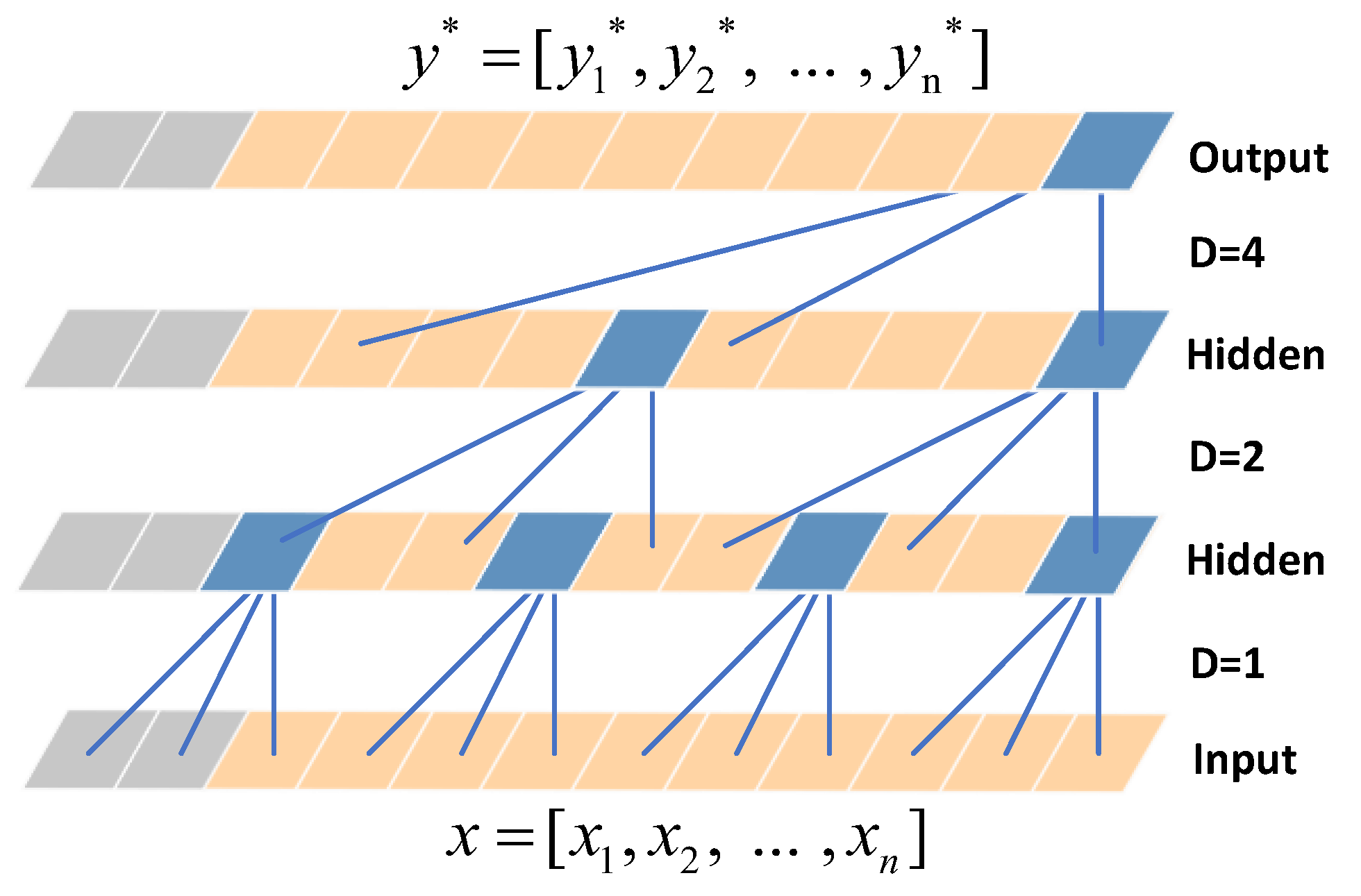
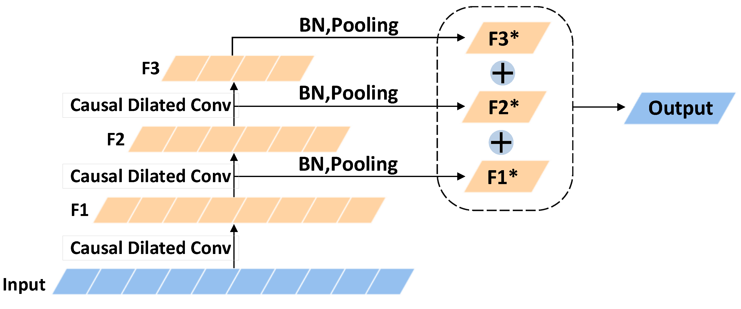
• A time series feature pyramid structure based on causal dilated convolution is proposed. Multiscale feature extraction and fusion are used to improve the prediction accuracy of the nonlinear model, which avoids the problem of insufficient feature extraction;
• A seasonal inflection month correction strategy is proposed. A unified model is constructed to predict and correct the seasonal inflection monthly load. It can overcome the problem of large model volume and improve the model’s ability to process and predict load seasonality;
• The method proposed in this paper is evaluated on the actual dataset, and the effectiveness and superiority of the method are verified with experiments.

2. Feature Pyramid CNN-LSTM Network

As will be explained in this section, the feature pyramid of the time series was constructed using causal dilated convolution, and it was applied to the CNN-LSTM tandem network to convolve load sequences with different receptive fields and thus extract feature information at different scales.

2.1. Causal Dilated Convolution

In recent years, causal dilated convolution has been applied to time series prediction. Compared with traditional convolution, the causal dilated convolution has strict time order constraints and a more flexible convolution kernel sampling interval, which could obtain a larger perceptual field without the information leakage in future time steps and more in line with the characteristics of time series data. It does not increase the network depth when extracting larger receptive field information, avoiding gradient disappearance and gradient explosion during training. This inspired us to investigate whether causal dilated convolution can be used to improve the CNN feature extraction module.

As shown in Figure 1, for the causal dilation convolution structure, the input time series x is outputted with the predicted value y* after a three-layer causal dilated convolution with dilation coefficients (1, 2, 4), and the traditional causal dilated convolution is characterized by outputting only the last layer of the feature map.

2.2. Feature Pyramid Structure of the Time Series

To extract the feature information of different time scales, the causal dilated convolution was used to construct a feature pyramid of the power load series, and the structure is shown in Figure 2. The input time series is convolved by three layers of causal dilated convolution to generate three time-scale feature maps of F1, F2, and F3. F1 is the feature of 3 adjacent time steps, F2 is the feature of 7 adjacent time steps, and F3 is the feature of 13 adjacent time steps. The outputs are F1*, F2*, and F3* after batch normalization and pooling. Then, these three feature maps are added to output fusion features. The feature pyramid realizes the extraction and fusion of features of different time scales.

2.3. Feature Pyramid CNN-LSTM Network

The feature pyramid CNN-LSTM hybrid neural network structure is shown in Figure 3. The prediction model consists of two parts: feature pyramid CNN and LSTM. The specific implementation analysis is presented in the following sections.

Feature pyramid CNN network consists of multiple one-dimensional causal dilation convolutional layers, pooling layers, and feature fusion units. Since the input–output sequences of the causal dilated convolution are of the same length, the input to each convolutional layer is $x=[x(1),x(2),...,x(t)]$, and the one-dimensional convolutional layer could be described as follows:

$$x_j^l=\mathrm{GELU}({\displaystyle \sum _{n=1}^N{x}_n^l{\ast }_d{f}_j^l+b_j^l}),$$

(1)

where $x_j^l$ denotes the output feature map of channel j in the lth convolutional layer, and $x_n^l$ is the nth input feature map of channel j in layer l. There are N input feature maps for this channel, $f_j^l$ is the weight of the convolution kernel of channel j in layer l, the causal dilated convolution is ${\ast }_d$, and $b_j^l$ is the bias of channel j in layer l. GELU is the activation function used in the convolutional layer:

$$\mathrm{GELU}(\mathrm{x})=x\mathrm{\Phi }(x),$$

(2)

Since $\mathrm{\Phi }(x)$ is difficult to calculate directly, the approximate function is as follows:

$$x\mathrm{\Phi }(x)\approx \frac{1}{2}x\left[1+\tanh \left(\sqrt{\frac{2}{\pi }}\left(x+0.044715x^3\right)\right)\right]$$

(3)

To capture multiscale temporal information, the convolution layer uses causal dilated convolution to enlarge the receptive field, and for element s in the input sequence, the convolution part of Equation (1) is defined as follows:

$$(x_n^{}{\ast }_d{f}_j^{})(s)={\displaystyle \sum _{m=0}^{k-1}{f}_{j,m}\cdot x_n(s-d\cdot m)}$$

(4)

where $x_n=[x_n\left(1\right), x_n\left(2\right) ,... ,x_n(t)]$ is the input vector, the convolution kernel is $f_j=[f_j\left(0\right), f_j\left(1\right), ... , f_j(k-1)],f_j\in {\mathrm{R}}^k$, the dilation factor is d, the kernel size is k, and $s-d\cdot m$ represents the direction of convolution.

The features extracted from each convolutional layer are sampled using a pooling layer to reduce the feature dimensionality. After the output feature map of channel j in the lth convolutional layer is maximally pooled, an element s in the output sequence could be described as follows:

$$u_j^l(s)=\max \{x_j^l(s\cdot r),x_j^l(s\cdot r+1),...,x_j^l(s\cdot r+(k-1))\}$$

(5)

where $x_j^l(s)$ is the element s of the output feature map of channel j in layer l, which is also the input of the pooling layer, r is the pooling interval, and k is the length of the pooling window.

The output features of all pooling layers are of the same size and contain different time-scale information, forming a feature pyramid, and the multiscale features are fused as the output of the CNN network. The output of channel j could be described as follows:

$$v_j={\displaystyle \sum _{l=1}^L{u}_j^l}$$

(6)

where $u_j^l$ is the pooled layer output feature map of channel j in layer l, and L is the number of convolutional layers of the feature pyramid CNN network and also the number of layers of the feature pyramid.

After that, the multiscale features extracted by the CNN network $v_j$ are input to the LSTM network for prediction. The LSTM network consists of three gates controlling the cell state to store long- and short-term memory. The sigmoid layer in the forget gate drops useless information from the previous moment and outputs a number between 0 and 1, representing the degree to which information has passed from the cell state of the previous moment into this moment:

$$f_t=\sigma \left(W_f\cdot \left[h_{t-1},v_t\right]+b_f\right)$$

(7)

The sigmoid and tanh layers in the input gate jointly determine the information to be stored in the cell state and update the cell state $C_t$:

$$i_t=\sigma \left(W_i\cdot \left[h_{t-1},v_t\right]+b_i\right),$$

(8)

$$C_t=C_{t-1}\ast f_t+i_t\ast \tanh \left(W_C\cdot \left[h_{t-1},v_t\right]+b_C\right).$$

(9)

The output gate determines the output information of the cell state through the sigmoid and tanh layers $h_t$:

$$o_t=\sigma \left(W_o\left[h_{t-1},v_t\right]+b_o\right),$$

(10)

$$h_t=o_t\ast \tanh \left(C_t\right).$$

(11)

In the above equations, $h_{t-1}$ is the output at the previous time step, $v_t$ is the input at this time step, $W_{}$ is the weight of each gate unit, and $b_{}$ is the bias of each gate unit.

Finally, the output state of the LSTM network is mapped to the final predicted output by a fully connected layer, as shown in Equation (12). In this equation, $H=[h_1,h_2,...,h_z]$ denotes the output vector of the LSTM network, and z is the number of LSTM network neurons. $W_d,b_d$ denotes the weights and biases of the fully connected layer.

$$p=\sigma (W_d\cdot H_{}+b_d)$$

(12)

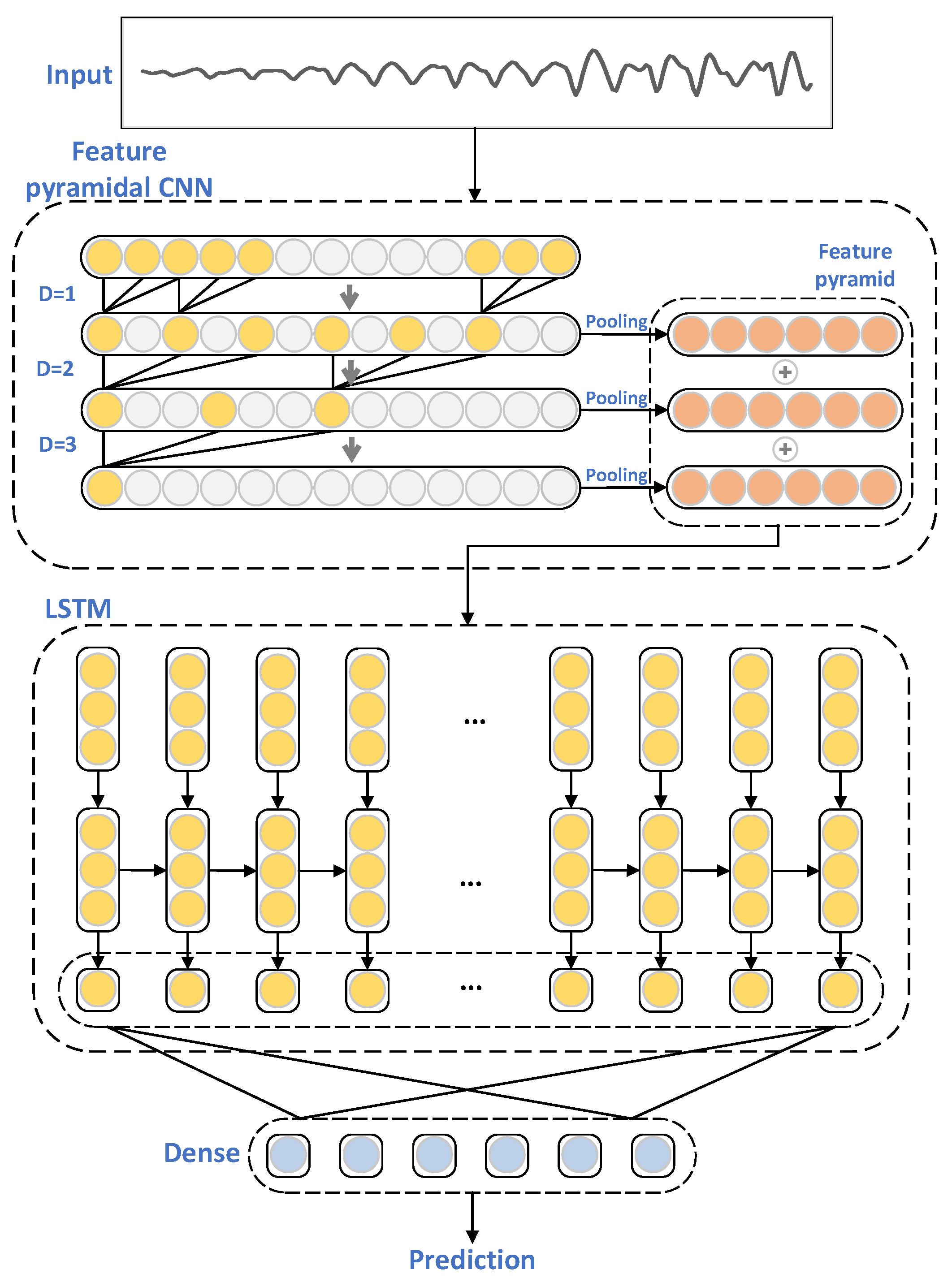
3. A Hybrid Feature Pyramid CNN-LSTM Neural Network Model Incorporating Seasonal Inflection Point Month Load Correction

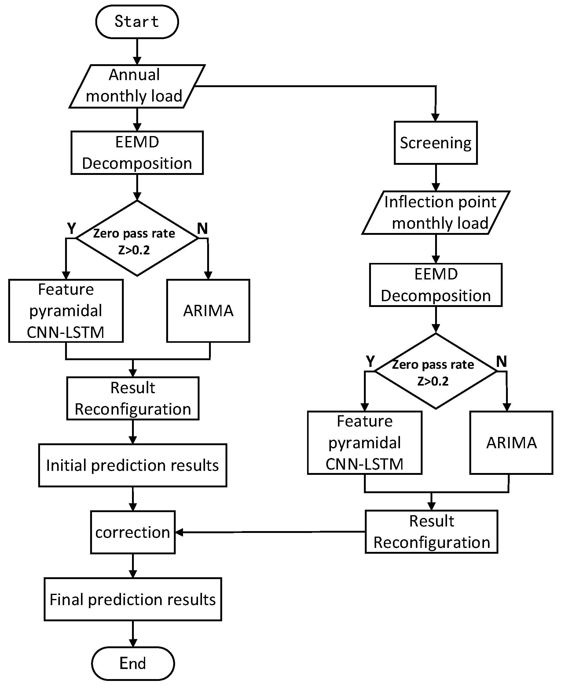
Electricity loads are influenced by climatic seasonal factors, which are highly volatile and difficult to forecast. To capture the complex volatility and temporal correlation in the power load sequence, we integrated the feature pyramid CNN-LSTM network with the inflection point monthly load correction to propose a medium- and long-term power load forecasting model (corrected feature pyramid EEMD-ARIMA-CNN-LSTM and CFPEACL), and the flowchart is shown in Figure 4.

The CFPEACL model is composed of two parts: the annual monthly load forecast and the inflection point monthly load correction. Based on the first part, the model is constructed separately by screening the seasonal inflection point monthly load, forecasting, and correcting the annual monthly load forecast results to obtain the final forecast output.

Both parts use the method of sequence decomposition combined with the construction of linear and nonlinear mixed models. First, the linear and nonlinear components of the electric load are separated using EEMD, where the high-frequency nonlinear components represent the strong random components of local features and noise, and the low-frequency linear components represent the overall trend of the load sequence. Then, each component is distinguished between high and low frequencies using zero-pass-rate detection, which is defined as follows:

$$Z=\frac{n_{zero}}{N}$$

(13)

where Z represents the over-zero rate, $n_{zero}$ represents the number of signal over-zero points, and N represents the signal length. In this paper, the threshold value of the zero pass rate was set to 0.2. Finally, the linear and nonlinear components are predicted using different models. The feature pyramid CNN-LSTM hybrid neural network is applied as a nonlinear model and ARIMA as a linear model, they are used to predict a series of IMFs obtained from EEMD decomposition separately. Since the components of EEMD decomposition are super-positioned with each other, the prediction results of each component with different frequencies are superimposed and reconstructed into load prediction results.

4. Experiment Analysis

The data used in this paper include both the monthly load data of Shaoxing City from January 1998 to December 2018 and its seasonal turnover data from 1961 to 2016. The performance of the proposed CFPEACL prediction model was validated and analyzed in three main aspects:

• Constructing a forecast study of the annual monthly load without inflection point monthly correction to verify the effectiveness of the feature pyramid EEMD-ARIMA-CNN-LSTM model (FPEACL);
• Constructing a separate model and forecasting the seasonal inflection point monthly load to verify the necessity of screening the inflection point monthly load forecasts;
• Using the results of the inflection point monthly load forecast to correct the initial annual monthly load forecast to output the global final forecast.

The proposed model was compared with the LSTM, EEMD-ARIMA (EA), EEMD-ARIMA-LSTM (EAL), EEMD-ARIMA-CNN-LSTM (EACL), EEMD-ARIMA-MultiCNN-LSTM (EAMCL), EEMD-TCN-LSTM (EATCL), and feature pyramid EEMD-ARIMA-CNN-LSTM models without correction for inflection point monthly load (FPEACL).

In order to compare the prediction accuracy and correlation performance of the proposed model and comparison models, evaluation metrics such as mean absolute percentage error (MAPE), mean absolute error (MAE), root-mean-square error (RMSE), and coefficient of determination (R²) were mainly used. For MAE and RMSE, the closer to zero means the smaller the prediction error, and the closer to 1 for R² means the better the fit, while MAPE needs to be compared between different models to be meaningful, and the smaller the value means the higher the prediction accuracy.

4.1. Annual Monthly Load Initial Forecast Analysis

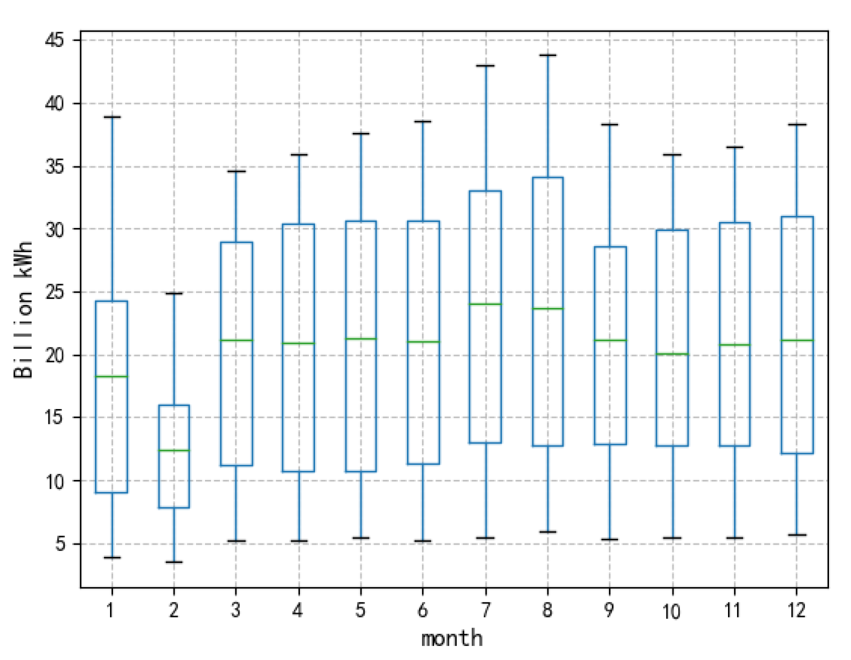
In this section, we mainly explain the verification process of the predictive validity of the FPEACL model. Before constructing the model, the data were first preprocessed. There were no missing values in our original data, but there were only the first six months of load in 2019. In order to equivalently evaluate the prediction accuracy of the model in each month, we deleted the final 2019 monthly load of the dataset. After that, as can be seen in the box–line diagram in Figure 5, the load data had no outliers and therefore could be used to fit the model.

The FPEACL modeling steps were as follows: Firstly, we decomposed the annual monthly load sequences using EEMD, and secondly, we performed zero-pass-rate detection for each component, and then the corresponding model predictions were performed for each component; finally, the initial prediction results were reconstructed and analyzed. The annual monthly load without inflection point month correction was predicted by using the load of the previous 12 months to forecast the load of the next 1 month, with a time window size of 12 and a move step of 1. The annual monthly load dataset was divided into the training set, the validation set, and the test set in the ratio of 8:1:1 to predict the monthly load from January 2017 to December 2018.

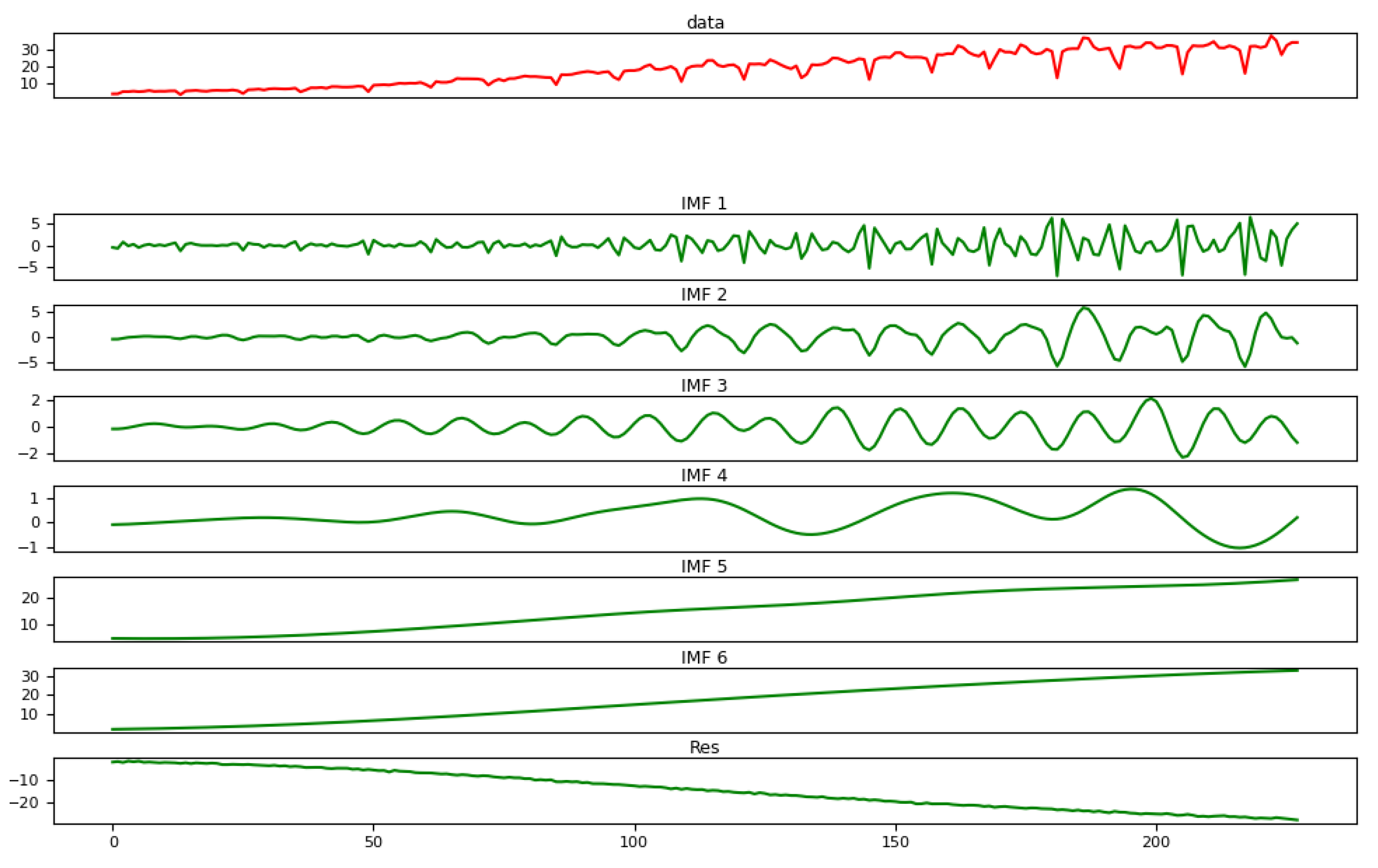
As shown in Figure 6, using EEMD, the training and validation sets of annual monthly load sequences were decomposed into seven IMFs containing a residual component. As shown in the figure, the red line is the original load, and the green lines are the components obtained by decomposition. After calculation, the zero pass rate of each component is shown in

Table 1. The zero-crossing rate of IMFS for monthly load training and validation sets.

IMF1	IMF2	IMF3	IMF4	IMF5	IMF6	Res
0.535714	0.198413	0.162698	0.027778	0	0	0

. The zero-crossing rate from IMF2 was lower than the threshold value of 0.2 set in this paper, and it can also be seen in Figure 5 that IMF1 had a high frequency and was extremely volatile; the components from IMF2 tended to level off and showed a strong periodicity; and IMF5, IMF6, and Res showed an extremely strong trend. Therefore, the feature pyramid CNN-LSTM hybrid neural network was used to predict the more complex pattern IMF1 and ARIMA to predict IMF2-6 and Res with a simpler pattern.

A series of IMFs obtained using EEMD decomposition were used to train the model and predict the IMFs from January 2017 to December 2018. The predicted results of each component were superimposed and reconstructed to obtain the initial predicted load results. In the experiment, the current FPEACL model was compared with the prediction results of the LSTM, EA, EAL, EACL, EAMCL, and EATCL models. The number of CNN layers of the four combined networks of CNN and LSTM is three, the size of the convolution kernel was three, the number of LSTM layers is two, and the number of LSTM neurons was (64,32). The details were as follows:

• CNN-LSTM: The input sequence was extracted using three one-dimensional convolution layers, and the feature map of the last layer was output to the LSTM to generate a prediction;
• MultiCNN-LSTM: The input sequence was extracted using three convolution layers with different convolution kernel sizes, and the feature maps of the three layers were added and fused to output to the LSTM to generate a prediction;
• TCN-LSTM: The input sequence was extracted using a TCN residual block, and then it was output to the LSTM to generate a prediction;
• Proposed method: The input sequence was extracted using three convolutional layers with different dilation rates, and the features of three different scales were added and fused to the LSTM to generate a prediction.

The ARIMA model parameters p, d, and q were determined using a grid search algorithm, and the best parameters for each component are shown in

Table 2. The best parameter combination of ARIMA, with p ranging from 0 to 12, and d and q ranging from 0 to 3.

	(p, d, q)
IMF1	(12, 0, 0)
IMF2	(6, 0, 1)
IMF3	(6, 0, 1)
IMF4	(3, 2, 1)
IMF5	(1, 2, 0)
IMF6	(0, 2, 1)
Res	(12, 1, 2)

.

All experiments were implemented in the same environment, and the details are shown in

Table 3. Software and hardware environment experiment parameters.

	Items	Parameters
Software	Operating System	Windows 10
	Experimental Platform	Anaconda 3
	Python	3.7
	TensorFlow	2.2.0
Hardware	CPU	AMD Ryzen 5 3550H
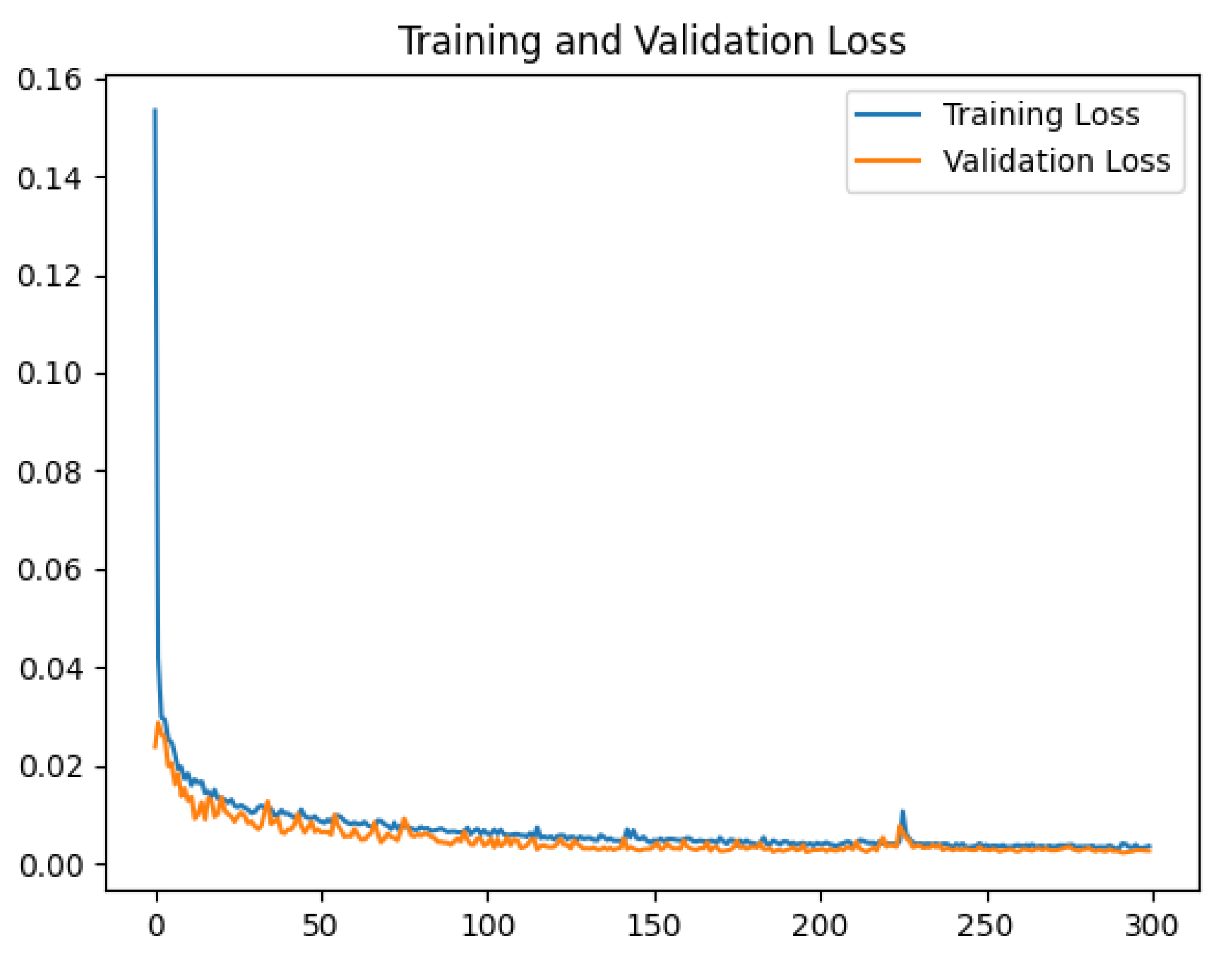
	CPU main frequency	2.10 GHz

. The training and verification losses of the proposed model are shown in Figure 7. The losses in these two datasets were slowly reduced to a small range during the iteration process, and the model had no overfitting or underfitting.

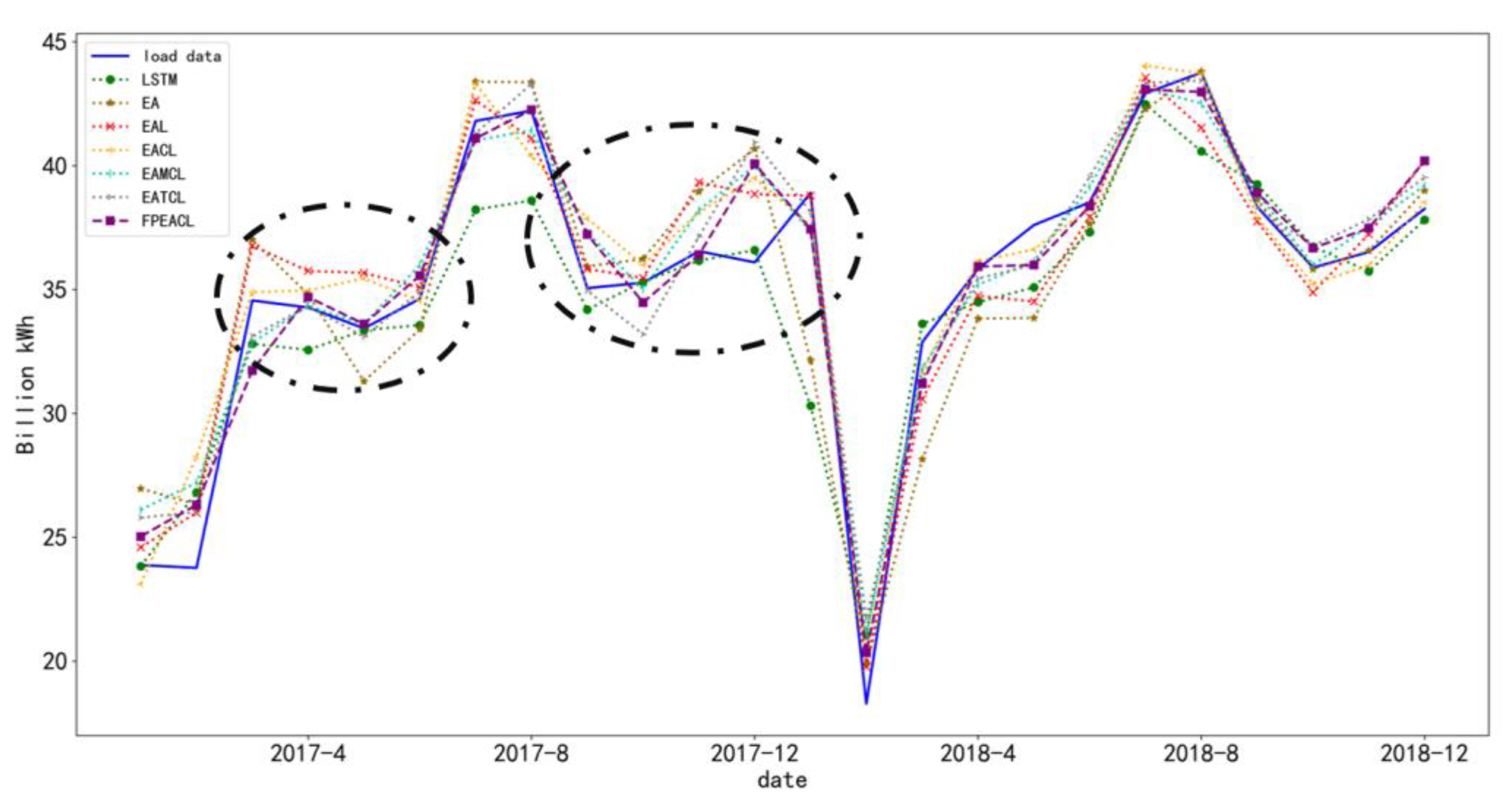
The annual monthly load initial prediction curve and indicators are shown in Figure 8. It can be seen from the figure that the overall prediction trend of the single LSTM model was in line with the real load characteristics, but the fitting was poor at the peak value in summer and the valley value during the Spring Festival. The EA model decomposed the original load and generated the ARIMA model prediction. The fitting of the real load trend was poor. The reason for this finding is that the ARIMA model has insufficient ability to deal with complex nonlinear components, and its nonlinear component prediction error is large; thus, the final fitting result of the hybrid model was not good. The three different types of CNN-LSTM combined networks had better prediction at peak and valley loads but had greater volatility, shown in black boxes. The proposed FPEACL method used CNN with a feature pyramid structure to extract the multiscale temporal correlation of load, which was best fitted with real load, but there were still large errors in individual months.

As shown in

Table 4. Comparison of monthly load initial forecast results indicators for the whole year between FPEACL and other models.

Model	MAPE	MAE	RMSE	R2
LSTM	4.910%	1.6848	2.4821	0.8230
EA	5.682%	1.8803	2.5110	0.8188
EAL	4.161%	1.3948	1.6847	0.8188
EACL	3.906%	1.2279	1.6400	0.9227
EAMCL	4.163%	1.2856	1.6367	0.9230
EATCL	3.875%	1.1830	1.6250	0.9241
FPEACL	3.967%	1.1713	1.5355	0.9322

, the LSTM, a commonly used neural network in time series prediction, had two LSTM layers to capture the long-short term features of the time series and a dropout layer to prevent overfitting. Better predictions were obtained using this model than using EEMD decomposition combined with the traditional statistical method in the ARIMA model. The EAL model used the neural network to predict the complex high-frequency components of the model. Compared with EA’s direct use of ARIMA to predict all components, the R² was equivalent, RMSE decreased by 34%, and MAPE decreased by 27%, indicating that the modeling prediction method based on different IMF component characteristics was effective. EACL, EAMCL, and EATCL used different CNN-LSTM combined networks to predict high-frequency components. Compared with EAL, the fitting degree was improved, and each error was reduced to varying degrees, indicating that the method of using CNN to extract features and LSTM prediction was effective. FPEACL used the feature pyramid CNN-LSTM hybrid neural network to predict the high-frequency component IMF1. Compared with the model based on other CNN-LSTM combined networks, MAPE, MAE and RMSE were the smallest in terms of error comparison. From the point of view of fitting degree, R² was closer to 1, and the predicted load was basically consistent with the actual data.

4.2. Inflection Point Monthly Load Correction Analysis

To further improve the forecasting accuracy, the CFPECAL method is proposed. The validity of the independent forecasts of monthly loads at seasonal inflection points was first verified, and then the initial forecasts were corrected using the monthly loads at seasonal inflection points to obtain the final global forecast output.

4.2.1. Seasonal Inflection Point Monthly Load Independent Forecast Analysis

The average time of season entry in Shaoxing City from 1961 to 2016, as well as the trend of significantly earlier spring and summer start dates and later autumn and winter start dates, were combined to identify the seasonal inflection months as March, May, September, October, November, and December. The seasonal inflection point monthly load independent forecast was determined using loads of the previous six months to forecast the load of the next month, with a time window size of six and a move step of one. The seasonal inflection point monthly load dataset was divided into a training set, a validation set, and a test set in the ratio of 8:1:1 to forecast the seasonal inflection point monthly load from 2017 to 2018.

The training and validation sets of the inflection point monthly load sequences were decomposed using EEMD, and the zero pass rates are shown in

Table 5. The IMF zero-crossing rates for monthly load training and validation sets at the seasonal inflection point.

IMF1	IMF2	IMF3	IMF4	IMF5	Res
0.6032	0.2619	0.0873	0	0	0

. While still separating the high-frequency components and low-frequency components according to the threshold 0.2, IMF1 and IMF2 were predicted using the feature pyramid CNN-LSTM hybrid neural network, and the rest of the components were predicted using ARIMA.

The parameters of the characteristic pyramidal CNN-LSTM hybrid neural network in seasonal inflection point monthly load independent forecasting were set as follows: The feature pyramid CNN network used two causal dilated convolutional layers with a kernel size of three and expansion factors of (1,2) so that the receptive field of the last convolutional layer can cover six seasonal inflection months of the year. The number of convolutional kernels was 48 for both convolutional layers. The LSTM network consisted of two LSTM layers with their neurons set as (48,32). The ARIMA model parameters p, q, and d were determined using a grid search algorithm.

The independent prediction results of the seasonal inflection point monthly load sequences were obtained after the prediction results of each component were superimposed and redetermined, and the results were compared and analyzed with the prediction results of the LSTM, EA, EAL, EACL, EAMCL, EATCL, and FPEACL using the models trained together with the load data of all months. The prediction curves and indicators are shown in Figure 7 and Table 4.

The combined results in Figure 9 and

Table 6. Comparison of independent load forecasting result indicators for the monthly seasonal inflection points.

Model	MAPE	MAE	RMSE	R2
LSTM	2.267%	0.8185	1.0561	0.5989
EA	5.448%	1.9206	2.5183	−1.2808
EAL	4.808%	1.7170	1.9654	−1.2808
EACL	3.517%	1.2451	1.5817	0.1002
EAMCL	3.507%	1.2587	1.6208	0.0552
EATCL	3.875%	1.1830	1.8089	−0.1768
FPEACL	3.715%	1.3300	1.8305	−0.2051
Independent FPEACL	1.642%	0.5869	0.7549	0.7950

show that for the seasonal inflection month loads, the prediction error was larger when training the model using year-round monthly load data. This may be due to high-temperature fluctuations and unexpected weather events in the seasonal inflection months, which caused load fluctuations and made it difficult to effectively capture the complex patterns in these months. By filtering the six seasonal inflection point monthly forecast results from the 12-month forecast results for the whole year and discussing them separately, it can be seen that the error metrics MAPE, MAE, and RMSE almost all fluctuated within the range around the composite metrics for the monthly loads for the whole year, while R² was much worse than the composite metrics for the 12-month period and even had negative values, implying a worse fit than the average forecast method. This shows that the seasonal inflection month forecasts obtained while ignoring the effect of seasonal changes on monthly loads were unreliable. In contrast, screening out the seasonal inflection months and training the model to predict them in a targeted manner yielded smaller errors and better fits.

4.2.2. Integrated Forecast Analysis Incorporating Monthly Load Correction at Seasonal Inflection Points

The method proposed in this paper is to first train the FPEACL model based on the annual load data and then separately train the FPEACL model using the seasonal inflection point monthly load data, and finally correct the initial load prediction results using the seasonal inflection point monthly load prediction results. The prediction results and errors of each model are shown in Figure 10 and

Table 7. The comparison between CFPEACL and other models of final annual monthly load forecasting results.

Model	MAPE	MAE	RMSE	R2
LSTM	4.910%	1.6848	2.4821	0.8230
EA	5.682%	1.8803	2.5110	0.8188
EAL	4.161%	1.3948	1.6847	0.8188
EACL	3.906%	1.2279	1.6400	0.9227
EAMCL	4.163%	1.2856	1.6367	0.9230
EATCL	3.875%	1.1830	1.6250	0.9241
FPEACL	3.679%	1.1713	1.5355	0.9322
CFPEACL	2.446%	0.7302	0.9835	0.9722

.

Figure 10 shows the comparison between the prediction results of the proposed model and other models, where the solid blue line is the real load and the black dashed line is the predicted load of the CFPEACL model. Compared with other models, the prediction results of the model proposed in this paper had a better fitting degree with real data. Compared with the FPEACL model, the CFPEACL model combined with the seasonal inflection point monthly load correction has higher prediction accuracy at the peak-valley value and the load value with small changes in the black box. In terms of error, compared with the LSTM, EA, EAL, EACL, EAMCL, EATCL, and FPEACL models, the MAPE of the model proposed in this paper decreased by 50%, 57%, 41%, 37%, 41%, 37%, and 34%, and the RMSE decreased by 60%, 61%, 40%, 40%, 40%, 40%, 39%, and 36%. In terms of the fitting degree, the R2 of the model proposed in this paper was the closest to 1, which was the best fitting with real data.

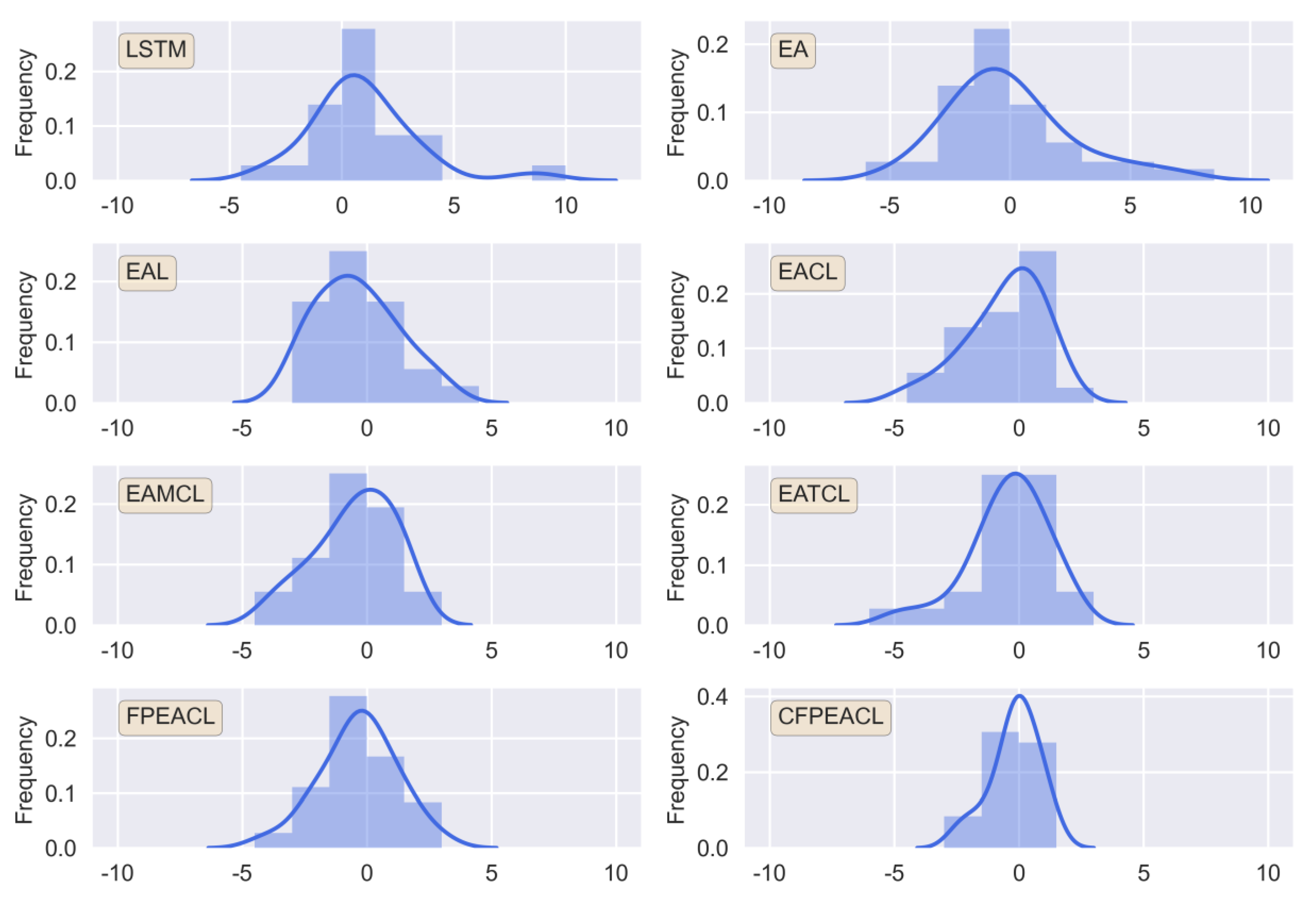
The error frequency histogram of each model is shown in Figure 11, where the curve represents the probability density of the residual. The higher the frequency of prediction error in the range of 0, the higher the prediction accuracy, and the better the stability of the model.

As can be seen from Figure 11, on the one hand, the single LSTM model could not effectively capture the random components in the load sequence, and on the other hand, it could not effectively extract the short-term local features within the sequence, so the model prediction accuracy and stability were poor. Although the EA model performed sequence decomposition, ARIMA could not fit the high-frequency components well, and the model performance was also poor. The EAL combined the advantages of LSTM and ARIMA well and compensated for the disadvantages of the first two models, and the prediction accuracy and stability were improved to some extent. EACL, EAMCL, and EATCL used convolution layers to extract the effectiveness of features in load sequences, and the prediction accuracy was somewhat improved. The FPEACL model used a feature pyramid CNN-LSTM hybrid neural network to extract features at different time scales, which further improved the model prediction capability. In this study, the inflection point monthly load correction was combined with FPEACL to propose the CFPEACL model, which could effectively capture the trend of seasonal change months, and the model stability and accuracy improved, as reflected in the optimal performance observed in the histogram of error frequency distribution.

In order to evaluate the complexity of the model, we compared the training time of the model.

Table 8. Model training time comparison.

Model	Time (s)
LSTM	185
EA	2483
EAL	1659
EACL	1805
EAMCL	1849
EATCNL	1820
FPEACL	1824
CFPEACL	2922

shows the comparison of the training time of all the models in this paper. The following data do not include the consumption time of hyperparameter tuning. It can be seen that the single LSTM model had the shortest time, while the training time of other hybrid models was basically 8–16 times that of the single model. The CFPEACL model proposed in this paper took the longest time to predict the final result because it contained the most components. The EA model was the second most time-consuming model because fitting the high-frequency components was difficult using ARIMA. The model duration of the four types of combined CNN and LSTM networks was not much different, because the number of combined network layers and hyperparameters used in this paper were almost the same.

5. Conclusions and Future Work

In this paper, a medium- and long-term power load forecasting model with a feature pyramid CNN-LSTM hybrid neural network was proposed to address the problems of the inadequate feature extraction of existing multiscale CNN networks, the difficulty of training optimization due to the complexity of the network, and the lack of consideration of the characteristics of electric load at seasonal change inflection points in forecasting. The electric load seasonality and nonlinearity were then analyzed by incorporating seasonal inflection point monthly load correction. Firstly, the power load series was decomposed using EEMD, and the low-frequency components were predicted using the ARIMA model. As for the prediction of the high-frequency components, causal dilated convolution was used to construct the feature pyramid structure of the power load series. It combined the CNN network to complete the multiscale feature capture at different levels within the components and input the fused features into the LSTM for prediction. Then, based on the analysis of the seasonal inflection point monthly load, the initial prediction results of the annual monthly load were modified using the seasonal inflection point monthly load correction to improve the model stability and prediction accuracy. Finally, the effectiveness of the proposed model was verified using the actual monthly electric load data of Shaoxing City for twenty years.

In the initial forecast of the annual monthly load without the correction of the inflection point monthly load, the proposed FPEACL model in this paper could obtain the smallest forecast error and the best fit with the original load compared with the LSTM, EA, EAL, EACL, EAMCL, and EATCL models, which verified the effectiveness of the feature pyramid CNN-LSTM hybrid neural network. In the forecast of the inflection point monthly load, six seasonal inflection point monthly forecast results were selected from the annual forecast results to verify the necessity of separate analysis for the seasonal inflection point monthly load. In the integrated prediction with the correction of the inflection point monthly load, the comparison experimental results show that the proposed model CFPEACL had the highest prediction accuracy, the best fitting effect, and stability.

In future work, we plan to use this method in other related areas, such as short-term load forecasting or electricity price forecasting, and verify the possibility and effectiveness of this method for other fields.