Article

Effect of a Vibrating Blade in a Channel on the Heat Transfer Performance

School of Energy and Environmental Engineering, Hebei University of Technology, Tianjin 300401, China
*
Author to whom correspondence should be addressed.
Energies 2023, 16(7), 3076; https://doi.org/10.3390/en16073076
Submission received: 28 February 2023 / Revised: 25 March 2023 / Accepted: 27 March 2023 / Published: 28 March 2023

Abstract

:
A vibrating blade was arranged in a channel to enhance heat transfer. The effects of the frequency and amplitude of the blade on the heat transfer characteristics were numerically researched. The phase space reconstruction and maximum Lyapunov index were used to analyze the transition path and degree of chaos. The results show that the vibrating blade can generate chaos; thus, the heat transfer is enhanced. The convective heat transfer performance is positively correlated with the degree of chaos. In addition, when the frequency is 10 Hz, and the inlet velocity is 0.5 m s−1, the heat transfer can be improved by 16%. When the maximum amplitude of the blade is 8 mm and the inlet velocity is 0.8 m s−1, the heat transfer can be improved by 15%.

1. Introduction

The study of chaotic convection has received increasing attention since the first introduction of chaos into fluid mechanics by Aref [1]. Chaotic convection is the phenomenon of turbulent diffusion in low Reynolds number laminar flows, which can effectively improve mixing efficiency. Burghelea et al. [2] studied chaotic flow and effective mixing of polymer solutions in microchannels by adding a small amount of flexible polymer. Tripathi et al. [3] investigated the mixing performance of a spiral micro-mixer based on chaotic advection under Dean flow conditions. The effect of pulsating flow and geometric disturbances on the mixing of laminar flow in a curved tube was investigated by Karami et al. [4]. Jarrahi et al. [5] used a combination of twisted tubes and pulsating flow to induce chaotic convection to enhance fluid mixing. Boyland et al. [6] and Balachandar et al. [7] studied stirred mixing in a three-dimensional vortex model to explore local Lagrangian chaos. Gepner et al. [8] studied chaotic mixing in low Reynolds number channels using surface ripple structures.
Identifying chaotic transition paths has always been an important direction in chaos research, reflecting the rhythmic changes that exist during the transition of a system from deterministic motion to chaotic motion. Yada [9] studied Rayleigh–Benard convection from different paths to chaos at low Prandtl numbers and explored paths from cycles and time cycles to chaos. Cimarelli and Angeli [10] studied how natural convection in a vertical channel transitions from a steady state to a chaotic state. Bhowmick et al. [11] explored the transition process of natural flow direction chaos caused by temperature differences in V-cavity. Brett et al. [12] proposed a new method for studying the advection of regular and chaotic fluids by studying stirrers. Many scholars have studied the generation path of chaos [13,14,15].
Chaotic convection enhances fluid mixing and can greatly improve fluid heat transfer characteristics. Two-dimensional closed pulsating heat pipes were studied and chaotically analyzed by Pouryoussefi et al. [16,17]. Ghaedamini et al. [18] studied the flow and heat transfer characteristics of a serpentine channel. The results showed that the corrugated structure in the channel could induce strong chaotic convection. The heat transfer capacity can be increased by 80%. The nonlinearity of critical heat flow in narrow channel natural circulation is analyzed by Cheng et al. [19]. Bahiraei et al. [20] found a more uniform cross-sectional flow velocity and temperature distribution. Guzman et al. [21] and Cristina et al. [22] studied the transition from converging and diverging channels to chaotic transition and the enhancement of chaos. It was found that special flow channels have a better contribution to heat transfer and mixing in comparison with the direct channel. Kang et al. [23] conducted a space experimental study on the oscillatory characteristics of hot capillary convection and chaotic transition paths in a circular liquid pool, and observed three kinds of transition paths, including quasi-periodic, period-doubling and parsmal bifurcation, and further discussed the mechanism of hot capillary force by comparing it with the buoyancy and thermal capillary convection in ground experiments. Chaotic coils can also induce chaotic enhanced heat transfer [24,25]. The generation of chaotic convection was verified by a large eddy simulation by Leonard [26]. The large eddy simulation method is further studied by Siddiqa et al. studied [27]. The influence of chaotic characteristics on the pulsating heat pipe is studied by Song et al. and Jing et al. [28,29]. The chaotic characteristics are judged by constructing the phase space trajectory and calculating the maximum Lyapunov exponent. The maximum Lyapunov exponent is obtained to increase with the increase of heating power, and the stronger the chaos, the better the heat transfer performance. The two-phase closed thermosiphon has a deterministic chaotic behavior, and the parameters used significantly affect the chaos and heat transfer performance. Chaos and heat transfer performance are positively correlated.
At present, electronic devices are developing towards miniaturization and integration. From the point of energy saving, energy consumption can be reduced by enhancing heat transfer. Several enhanced heat dissipation methods have been proposed, e.g., fins [30], nano-fluids [31], and twisted tubes. However, air cooling is still the dominant method for heat dissipation from electronic devices. Vibrating fans have been gaining attention recently due to the advantages of low noise and power consumption. Liu et al. [32] studied the effect of the placement of vibrating fans in large spaces on heat transfer. Lin [33] investigated the effect of the vibration of vibrating fans on heat dissipation from a cylindrical heat source. Shyu [34] studied the heat transfer effect of different positions of vibrating fans on plate fins and needle fins. The results showed that the heat transfer effect of the vibrating fan is related to its arrangement and position. Ding and Liu [35] studied the effect of distance on the heat dissipation characteristics of the vibrating fan. They reported that too small a distance reduces heat transfer characteristics. Lin et al. [36,37,38] applied a vibrating fan to a column-fin heat sink and analyzed the surrounding flow field distribution. Tan et al. [39] carried out two-dimensional numerical simulations of the flow field generated by a vibrating fan. The results showed that the jets formed by the vibrating fan have an enhanced heat transfer effect, with the best-enhanced heat transfer effect where the vortex breaks and the degree of fluid turbulence is strongest. Lin et al. [40] carried out a detailed analysis of the three-dimensional flow field around the vibrating fan. The flow field showed that the vibrating fan could generate longitudinal and lateral airflows, and their interaction formed a pair of opposite vortices. Kim et al. [41] applied the Q criterion to identify the vortical structure formed by the fan blade in the channel. The results showed that the vortical structure carries most of the kinetic energy, thus enhancing the heat transfer in the channel. Choi et al. [42] experimentally and numerically investigated the flow field induced by a vibrating fan. The changes in vortex nucleus migration trajectories and vortex size during vortex formation were captured. Sufian et al. [43,44] investigated the flow fluid and heat transfer characteristics under the effect of a flapping jet of double vibrating fans. The analysis focused on the formation and migration processes of reverse vortices.
As mentioned above, most research has been conducted on the vortices formed by vibrating fans. Previous research has reported that vortices could enhance heat transfer. The mechanism of enhanced heat exchange needs to be further revealed. It has been concluded that chaotic convection can enhance heat transfer. The analysis of the enhanced heat transfer mechanism of a vibrating fan from a chaotic perspective is a completely new perspective. In the present work, a vibrating blade is arranged in a channel to enhance the convection heat transfer. Different blade frequencies and amplitudes are considered. The effects of frequency and amplitude on chaotic convection are analyzed through qualitative and quantitative methods, such as reconstructing the phase space and calculating the maximum Lyapunov exponent for nonlinear systems. The chaotic characteristics are analyzed to reveal the mechanism of heat transfer.

2. Methodology

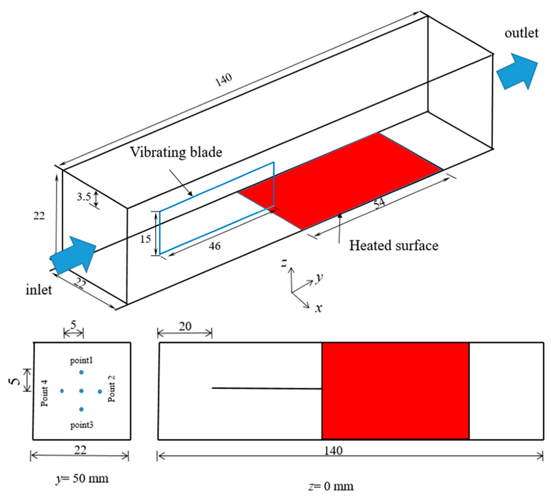
2.1. Computational Domain

The computational domain is a rectangular channel with 140 mm length, 22 mm width, and 22 mm height, as shown in Figure 1. A rectangular vibrating blade with 46 mm length, 15 mm width, and 0 mm thickness is arranged in the channel. The heated surface is 54 mm in length. In addition, four points in the y = 50 mm section are shown in the figure, which is used to monitor the time series later.

2.2. Governing Equations and Boundary Conditions

Continuity equation:
ρ t + x i ( ρ u i ) = 0 .
Momentum equation:
t ( ρ u i ) + x j ( ρ u i u j ) = p x j + τ i j x j + ρ g i + F i .
Energy equation:
t ( ρ c p T ) + x j ( ρ u i c p T ) = k 2 T x j 2 ,
where cp, k, and T denote the specific heat, thermal conductivity, and temperature of the air, respectively.
According to the research [45], the k-ω SST turbulence model is adopted, i.e.,
t ( ρ k t ) + x j ( ρ k t u i ) = x j + ( Γ k k t x j ) + G k Y k ,
t ( ρ ω ) + x j ( ρ ω u i ) = x j + ( Γ ω ω x j ) + G ω Y ω + D ω ,
where Gk and Gω denote the turbulent kinetic energy and the generic term of ω, respectively; Yk and denote the turbulent kinetic energy dissipation term and the specific dissipation rate, respectively; Γk and Γω denote the effective diffusivity of kt and ω, respectively; and Dω is the cross-diffusion term.
The constant air velocity boundary condition is adopted for the channel inlet. The inlet velocity is 0.5 m s−1, 0.8 m s−1, and 1.0 m s−1, respectively. The pressure outlet boundary condition is adopted for the channel outlet. The constant heat flux boundary condition is adopted for the heated surface, which is 1500 W m−2. For transient simulation of fan blade reciprocating vibrations, a larger time step results in worse mesh quality and reduces the accuracy of the simulation. In contrast, a smaller time step results in longer computational cycles [45]. After several tests, 1.0 × 10⁻³ s was selected as a time step size in the present work. The SIMPLE algorithm is used to solve the coupling between pressure and velocity. The second-order upwind discretization scheme is adopted for all terms except diffusion terms.

2.3. Data Reduction

Some parameters were defined to analyze the characteristics of heat transfer and fluid flow. The Reynolds number Re is defined as:
R e = ρ v inlet D h μ ,
where vinlet is the inlet velocity of air, m s−1; Dh is the equivalent diameter of the inlet, m; ρ is the density of air, kg m−3; and μ is the dynamic viscosity of air, kg m−1 s−1.
The Nusselt number Nu is defined as:
N u = h D h λ ,
h = q h Δ T ,
where λ is the thermal conductivity of air, W m−1 K−1; h is the convection heat transfer coefficient, W m−2 K−1; qh is the heat flux of the heated surface, W m−2; and ΔT is the temperature difference between the heated surface and the air, K.
The dimensionless amplitude Da is defined as the ratio of the maximum amplitude of the blade A and the equivalent diameter of the inlet Dh, i.e.,
D a = 2 A D h ,
The enhanced heat transfer factor Eh is defined as:
E h = h v h 0 ,
where the subscript v and 0 mean the channel with a vibrating blade and without a vibrating blade, respectively.
As shown in Figure 1, an xy coordinate system was established to fit the vibration curve of the vibration section of the blade. The amplitude at a different position is expressed as:
A ( y ) = ( y 72 ) 2 × 1.175 A ,
where y is the coordinate value in line with the direction of the fan blade length, and A is the maximum amplitude of the fan blade.
According to the results of the vibration test, the trajectories of the blade are expressed as follows:
x ( y , t ) = A ( y ) sin ( 2 π f t ) .
To determine the chaos in the system, the maximum Lyapunov exponent is defined below. A column of time series is selected for phase space reconstruction. The correlation dimension and delay time can be calculated. Then, the Lyapunov exponent can be obtained. The time delay τ and embedding dimension m of the system are determined by the Takens theory. Single variable time sequences are x1xn−1, xn. The phase space is reconstructed as follows:
Y ( t i ) = x ( t i ) , x ( t i + τ ) , x ( t i + 2 τ ) , x ( t i + ( m 1 ) τ ) i = 1 , 2 , , M , M = n ( m 1 ) τ
C ( τ ) = 1 N j = 1 N ( x j + τ x ¯ ) ( x j x ¯ ) 1 N j = 1 N ( x j x ¯ ) 2 ,
G m = j = 1 M Y j ( m + 1 , τ ) Y j ( m , τ ) = j = 1 M ln x j , m + 1 x j 0 , m + 1 x j , m x j 0 , m ,
d j ( 0 ) = Y j Y j 0 ,
d j ( i ) = Y j + i Y j 0 + i ,
y i = 1 q Δ t j = 1 q ln d j ( i ) ,
where Y is the reconstructed phase space; m is the embedded dimension; n is the number of time sequences; C(τ) is a linear autocorrelation function; x ¯ is the average of the data; τ corresponding to the delay time when C(τ) is 1 1 e for the first time is the delay time; G(m) is the ratio of higher dimensional phase space to lower dimensional phase space; j is the number of points in phase space; i is the separation time step; Yj is the point of phase space; Yj0 is the nearest point of Yj; dj(0) is the distance between Yj and Yj0; q is the number of non-zero dj(i); and y(i) is the average value of ln[dj(i)]. The slope of the regression line made by the least square method is the maximum Lyapunov exponent [46,47].

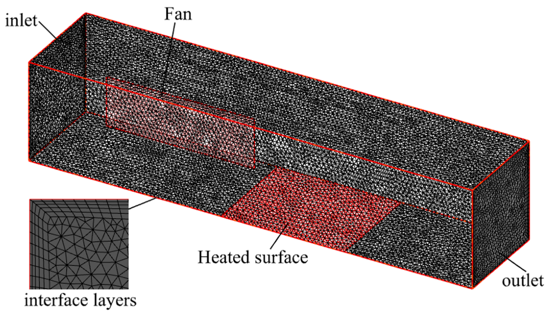
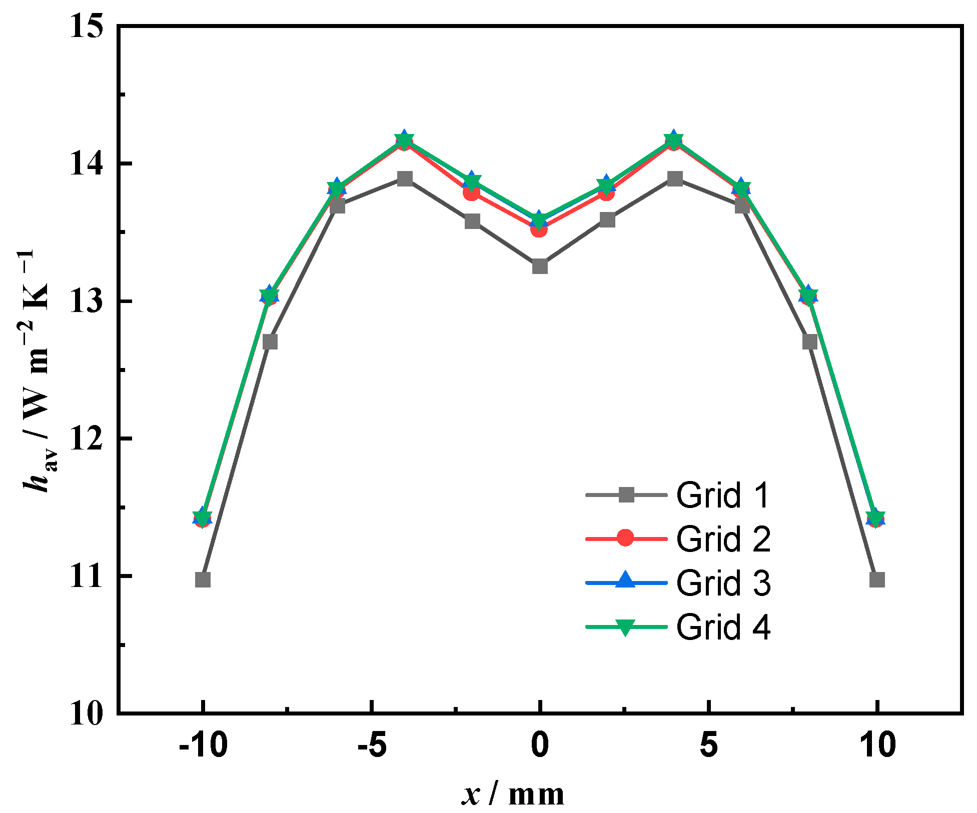
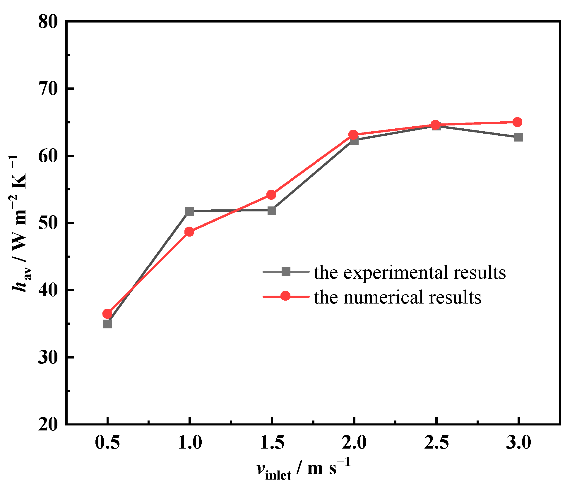
2.4. Grid Independence Validation and Model Validation

The computational domain mainly used a tetrahedral grid, as shown in Figure 2. Five inflation layers were used near the heated surface for better temperature and velocity gradients. The length of the first layer of the grid is kept at 0.1 mm to ensure that y+ is less than 1. Two dynamic mesh methods, smoothing and remeshing, were used to achieve the oscillation of the blade. To save calculation time, the grid independence of the model was verified, as shown in Figure 3. The number of grids was 302,050, 398,043, 502,530, and 701,576, respectively. The average convective heat transfer coefficient along the x-direction was compared. The convective heat transfer coefficient is stable when the number of grids exceeds 500,000.
To verify the accuracy of the model, the numerical results were compared with the experimental results from the literature [48], as shown in Figure 4. The computational model used for validation remained consistent with the experiments in the literature [48]. The average convective heat transfer coefficients at the heated surface for different channel inlet velocity conditions were compared. The general agreement between the numerical and experimental results confirmed the accuracy of the simulations.

3. Analysis of Heat Transfer Characteristics

Heat transfer analysis of a vibrating fan with different frequencies and amplitudes is shown in Figure 5. The enhanced heat transfer coefficient is defined as the ratio of the heat transfer coefficient when the fan blade is vibrating to no vibration. The effect of the natural frequency of the blade at A = 5 mm on the heat transfer performance is shown in Figure 5a. The effect of the amplitude of the blade at f = 5 Hz on the heat transfer performance is shown in Figure 5b. When the frequency is 10 Hz, the heat transfer can be improved by 16%. When the maximum amplitude of the blade is 8 mm, the heat transfer can be improved by 15%. This indicates that a larger frequency or amplitude is beneficial to improve heat transfer at the same inlet velocity.
Figure 6 shows the variations of the Nusselt number (Nu) with the dimensionless amplitude (Da) for different Re. The growth rate of Nu increased significantly when the dimensionless amplitude was greater than 0.272. The reasons for Re and dimensionless amplitude (Da) for enhanced heat transfer will be analyzed in Section 4.3.
The temperature distribution or flow field is used to further reveal the mechanism of the heat transfer performance of the channel with the vibrating blade. As mentioned above, the greatest heat transfer enhancement is obtained at f = 10 Hz and A = 5 mm. Figure 7 shows the temperature distribution of the heated surface at f = 10 Hz and A = 5 mm. The figure also shows two cases of without a blade and blade swing to maximum amplitude (Phase π/2). It can be found that the symmetrical ripple-shaped temperature contour is obtained for the channel without a blade. The higher temperature in the region close to the channel outlet is due to the gradual heating of the airflow and the gradual thickening of the boundary layer. For the channel with a blade, W-shaped temperature contours are obtained. Especially, the low-temperature region is larger due to the disturbance of the blade.
The variation of the instantaneous velocity vector with a phase of the z = 0 mm section is shown in Figure 8. When the phase of the blade is 0π, π, and 2π, vortices are formed on both sides of the blade tip. When the phase of the blade is π/2 and 3π/2, the position of the vortex moves forward. Vortices on both sides are generated constantly because of the vibration of the fan blade. The blade alternates on both sides to form a vortex and extend continuously forward. It can be considered that the constant variation of the vortices leads to the irregular temperature distribution in Figure 7.
As the vibration of the blade forms vortices at the blade tip, the instantaneous velocity vectors of different phases at the y = 50 mm section are shown in Figure 9. The contour indicates that two primary vortices are generated at the cross section. The direction of the vortex changes with the vibration of the blade, but the two vortices are always in opposite directions. When the blade vibrates to the phase of π/2 and 3π/2, the cross-sectional velocity is higher, and a pair of significant reverse vortices are formed. When the blade vibrates to the phase of π and 2π, the cross-sectional velocity is lower, and the vortices become less obvious. The main reason is the more intense disturbance effect of the blade on the airflow when the blade is in the maximum amplitude position.
From the above analysis, it can be considered that the vortices formed by the vibrating blade result in a higher heat transfer. Next, the enhanced heat dissipation mechanism is analyzed from a chaotic perspective.

4. Analysis of Chaotic Characteristics
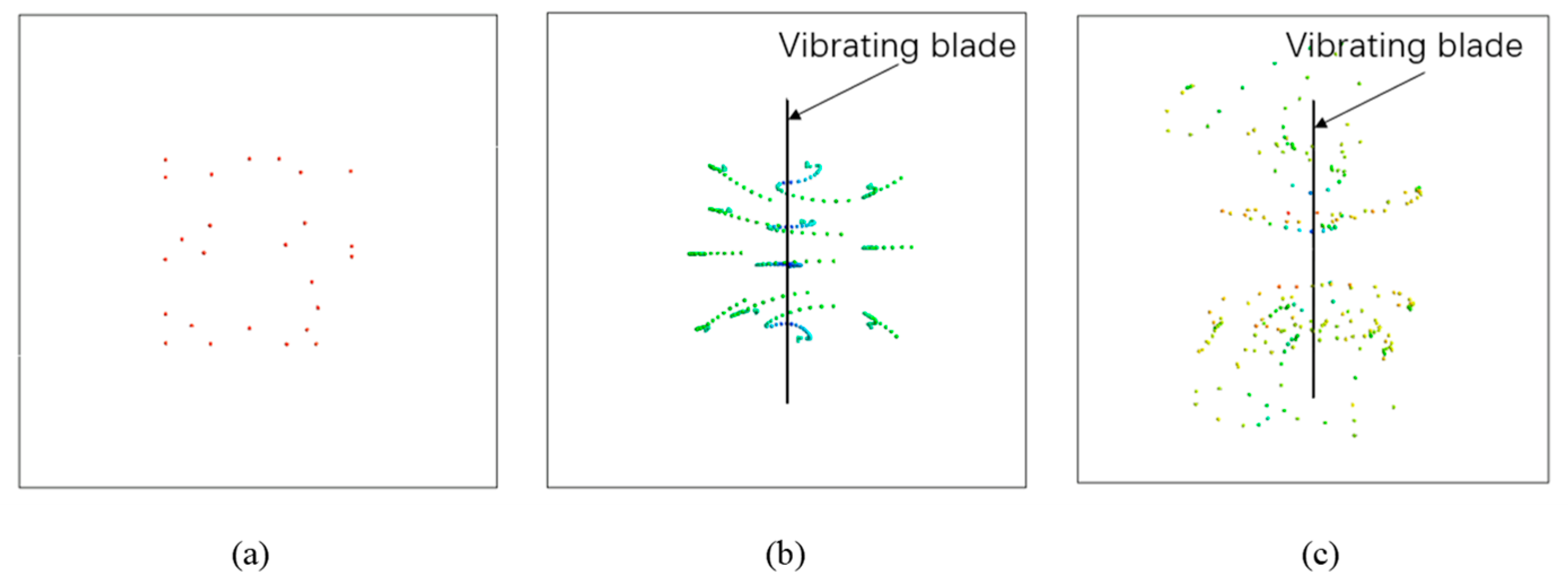
In this section, the chaotic characteristics of the flow field generated by the vibrating blade are discussed to reveal the mechanism of the heat transfer enhancement. The Poincaré map, power spectral density, phase space reconfiguration, and maximum Lyapunov exponent are analyzed as follows.

4.1. Poincaré Map

The Poincaré map is a dimensionality reduction process. It is possible to see that the advection problem can be reduced to a finite-dimensional dynamical system from a Lagrangian point of view. The traces are the trajectories of massless particles in the fluid field. A Poincaré map can be obtained by mapping fluid particles traversing multiple planes to the intersection of the planes. The Poincaré map can be generated by crossing a plane and the path line of the fluid particles, as shown in Figure 10. A number of 20 massless particles are released from the inlet for vinlet = 0.5 m s−1 to create a Poincaré map, as shown in Figure 11. It can be found that the particles are concentrated in the middle region without diffusion for the channel without a blade. The chaos is found when f = 5 Hz and A = 5 mm. When f = 10 Hz and A = 5 mm, strong chaos is found. This reveals that the vibrating blade significantly generates chaos.

4.2. Power Spectral Density

The velocity component w in the z-direction of the vibrating blade without inlet velocity is plotted with time, as shown in Figure 12. It can be found that the velocity becomes increasingly chaotic with increasing frequency. The power spectral density is obtained by Fourier transformation, as shown in Figure 13. The power spectral density diagram can be used as a basis for determining the generation of chaos. The power spectrum density at different frequencies is analyzed. The power spectrum of periodic motion is a discrete spectrum; the power spectrum of chaotic motion is a continuous spectrum. More than four incommensurable frequencies are in the power spectrum, indicating that the system has reached a chaotic state. The system is in a periodic state when the vibrating frequency is 3 Hz. When the vibrating frequency is over 5 Hz, this indicates that the system has reached a chaotic state.

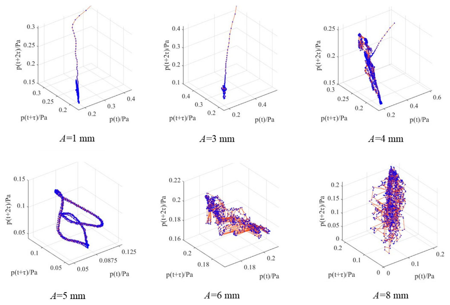
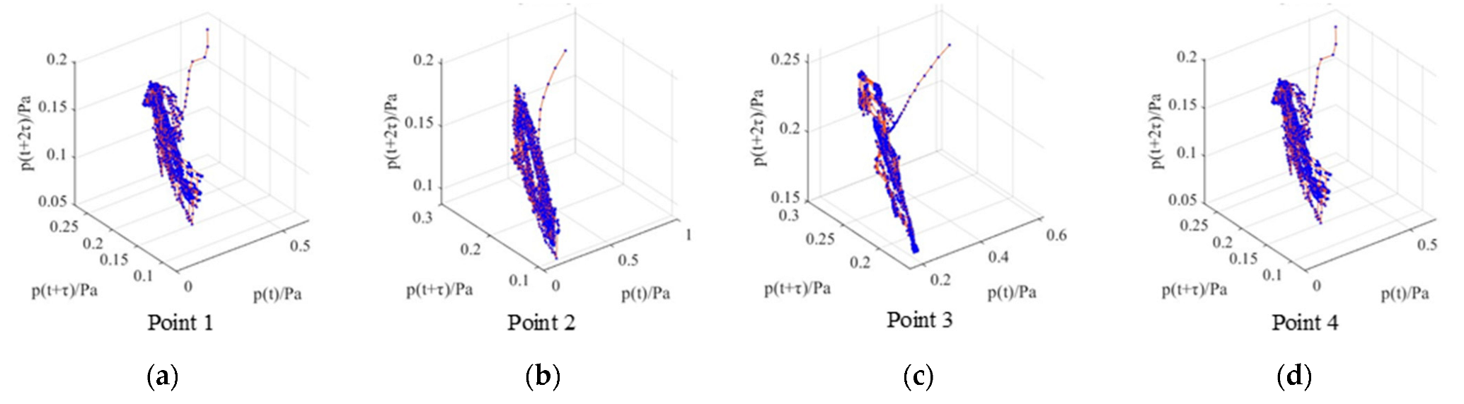
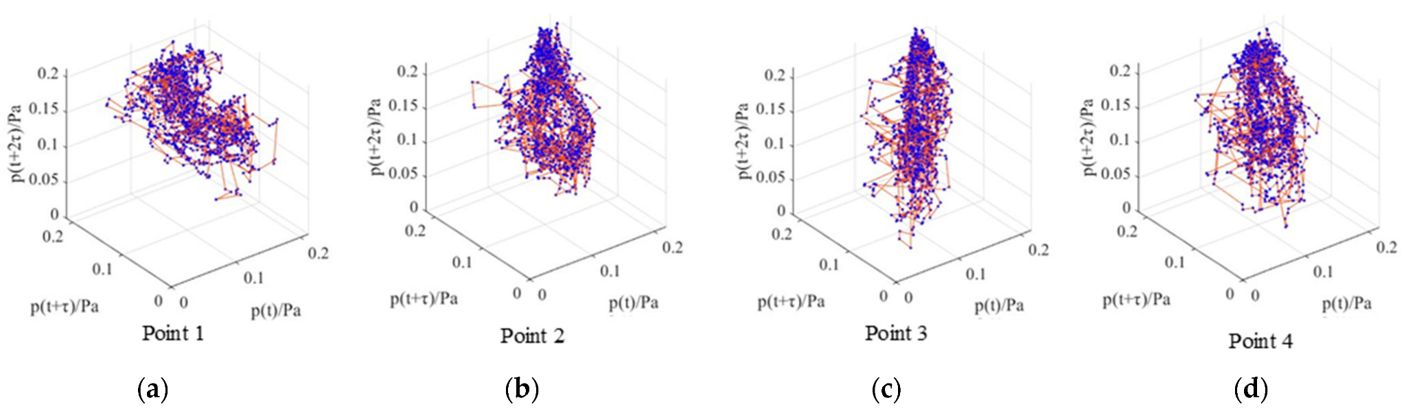
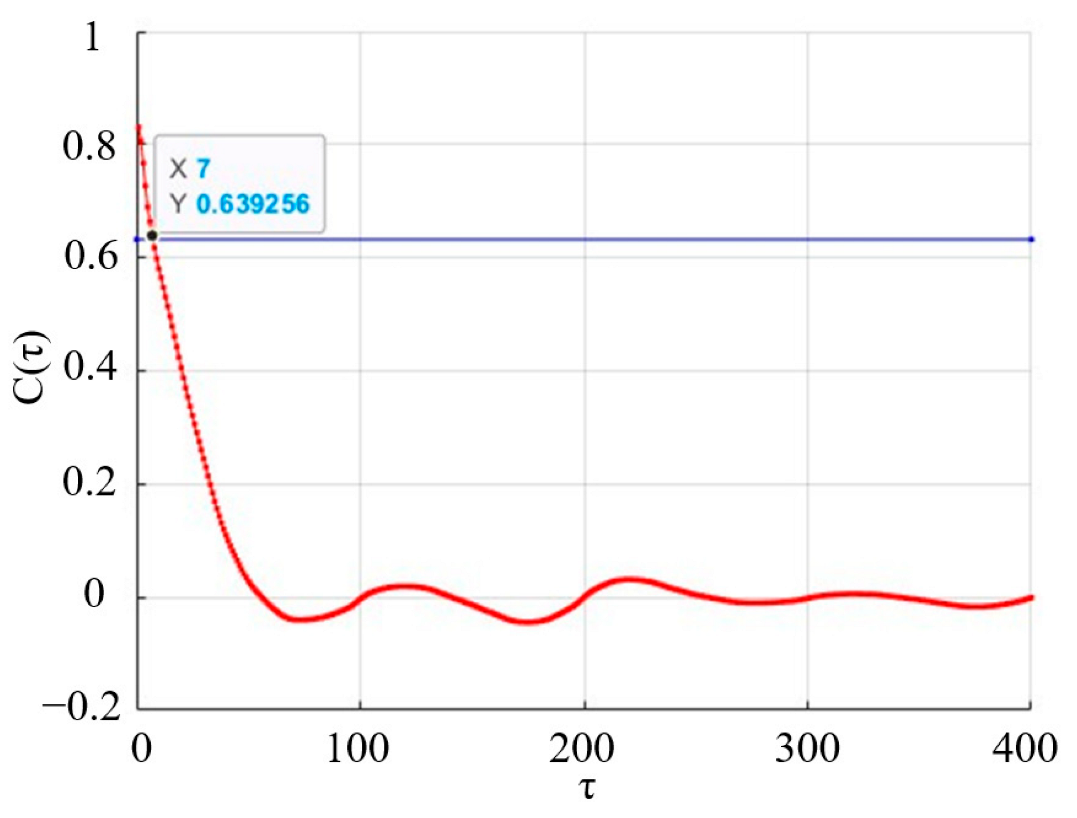
4.3. Phase Space Reconfiguration

Attractors are formed by the separation and folding of trajectories in phase space when the system is in chaotic motion. Attractors have complex and unique properties and are often called strange attractors for chaotic motion. The phase space reconstruction at different amplitudes is shown in Figure 14. It can be found that the phase space has an elongated linear shape as the amplitude decreases. The system first reaches a periodic state and then gradually reaches a chaotic state as the amplitude increases. The attractor phase diagram for periodic motion should be a regular band. Chaotic attractor phase diagrams are irregular. The attractors converge in space and are concentrated in a fixed region. As shown in Figure 14, the chaotic state is displayed when the amplitude is 4 mm. The periodic state is returned when the amplitude is 5 mm. The final chaotic state is reached when the amplitude is 6 mm. With a further increase in amplitude, the degree of chaos becomes more violent when the amplitude is 8 mm.
The effect of the position of the four monitoring points on the chaotic characteristics in Figure 15 is explored. Figure 14 has determined the transition path of chaos. When the amplitudes of 4 mm and 8 mm were selected, it represented that the chaotic state was more representative. Phase space reconstruction was carried out at the other four points. When the amplitude is 4 mm, the phase space tracks of four monitoring points are shown in Figure 15. The phase space tracks of different monitoring points are roughly consistent. All points show a weak chaotic state. When the amplitude is 8 mm, the phase space tracks of the monitoring points are shown in Figure 16. Each monitoring point showed a strong chaotic state, indicating that chaotic convection was generated in the system.
Based on the power spectral density and the phase space reconstruction of the attractor trajectory, it can be concluded that the vibrating blade can effectively generate chaos. The convective heat transfer coefficient increases slowly before the chaotic state is created. The heat transfer is significantly increased when the system reaches a chaotic state.

4.4. Maximum Lyapunov Exponent

The Lyapunov exponent is an important indicator for determining whether a system has reached chaos or not. The presence or absence of chaos in a system can be intuitively determined by whether the maximum Lyapunov exponent (MLE) is greater than zero [49,50,51,52]. The calculation of the maximum Lyapunov exponent begins with a phase space reconstruction of a time series of pressure, velocity, temperature, etc. Phase space reconstruction is the construction of a primary dynamical system from a component of the system. In the present work, the pressure time series is adopted.
The relevant dimension and the maximum Lyapunov exponent are calculated by Equations (14), (15), and (18). The delay time is shown in Figure 17. The autocorrelation coefficient of chaotic systems decreases with time. When the autocorrelation coefficient reaches 1 1 e for the first time, the horizontal coordinate at this point is the delay time. The relevant dimensions are shown in Figure 18. The correlation dimension is a quantitative description of a chaotic system. When the number of embedded dimensions m is increased to a certain level, the correlation dimension of a chaotic system converges to a more stable value. When the ratio of the high-dimensional phase space to the low-dimensional phase space no longer varies and tends to equilibrium, the horizontal coordinate is the number of embeddings. After determining the delay time and the embedding dimension, the Lyapunov exponent is calculated. The maximum Lyapunov exponent at f = 10 Hz is shown in Figure 19. The slope of the curve denotes the maximum Lyapunov exponent. The maximum Lyapunov exponent is 1.732 at f = 10 Hz and A = 5 mm. At this moment, the delay time is 7, and the embedding dimension is 25. Calculating the maximum Lyapunov for the other operating conditions in the same way as above shows the maximum Lyapunov exponent is 1.1458 for vinlet = 0.8 m s−1, f = 7 Hz, and A = 5 mm. The maximum Lyapunov exponent is 1.1269 for vinlet = 1.0 m s−1, f = 7 Hz, and A = 5 mm. Obviously, the degree of chaos is greater when the inlet velocity is 0.8 m s−1.

5. Conclusions

The heat transfer characteristics of a channel arranged with a vibrating blade are numerically investigated. The effects of the natural frequency and the amplitude on the heat transfer performance are analyzed. The chaotic characteristics of the airflow induced by the vibrating blade are further investigated. The main conclusions are as follows.
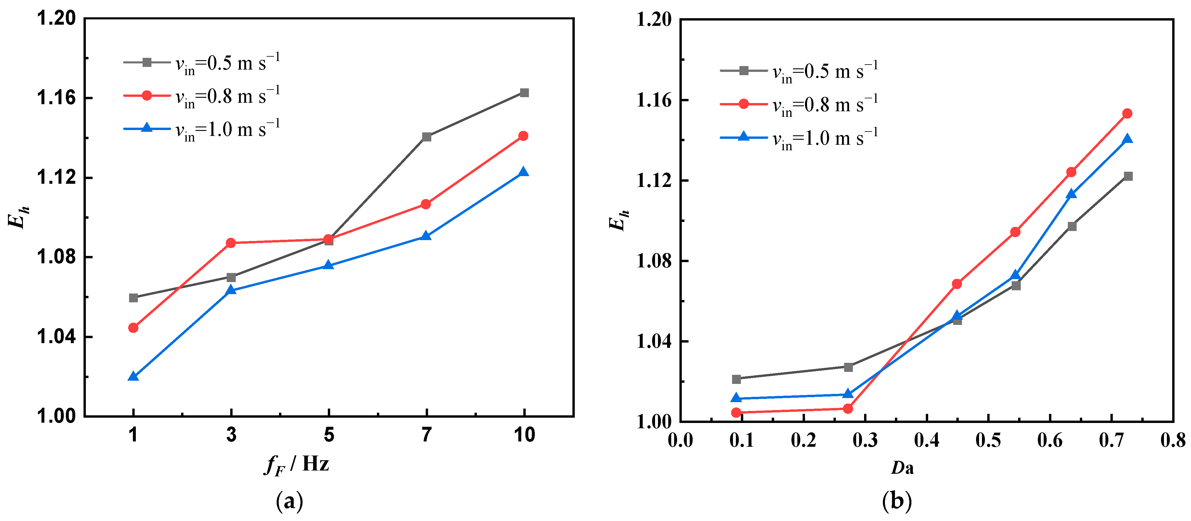
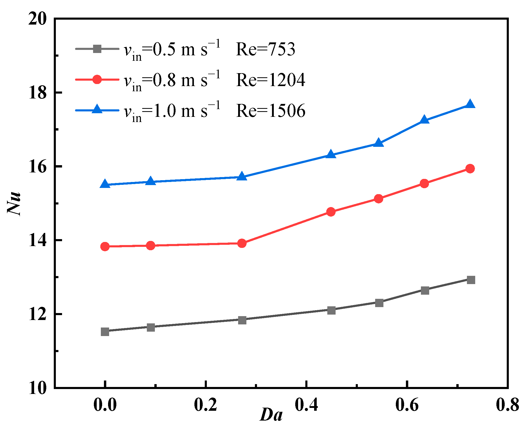
  • A larger frequency or amplitude is beneficial to improve heat transfer at the same inlet velocity. When the frequency is 10 Hz, the heat transfer can be increased by 16%. When the maximum amplitude of the blade is 8 mm, the heat transfer can be increased by 15%.
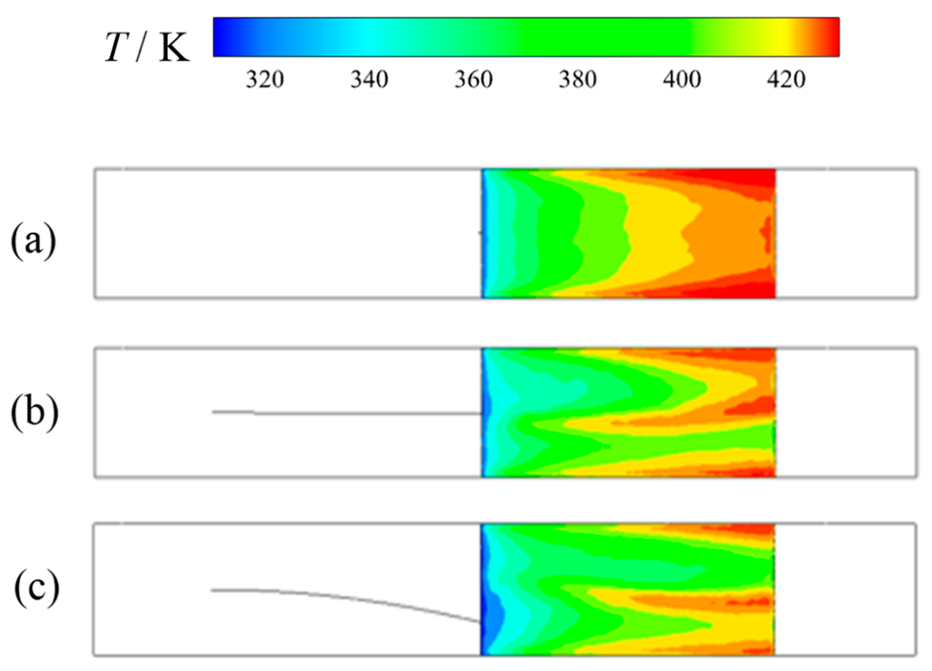
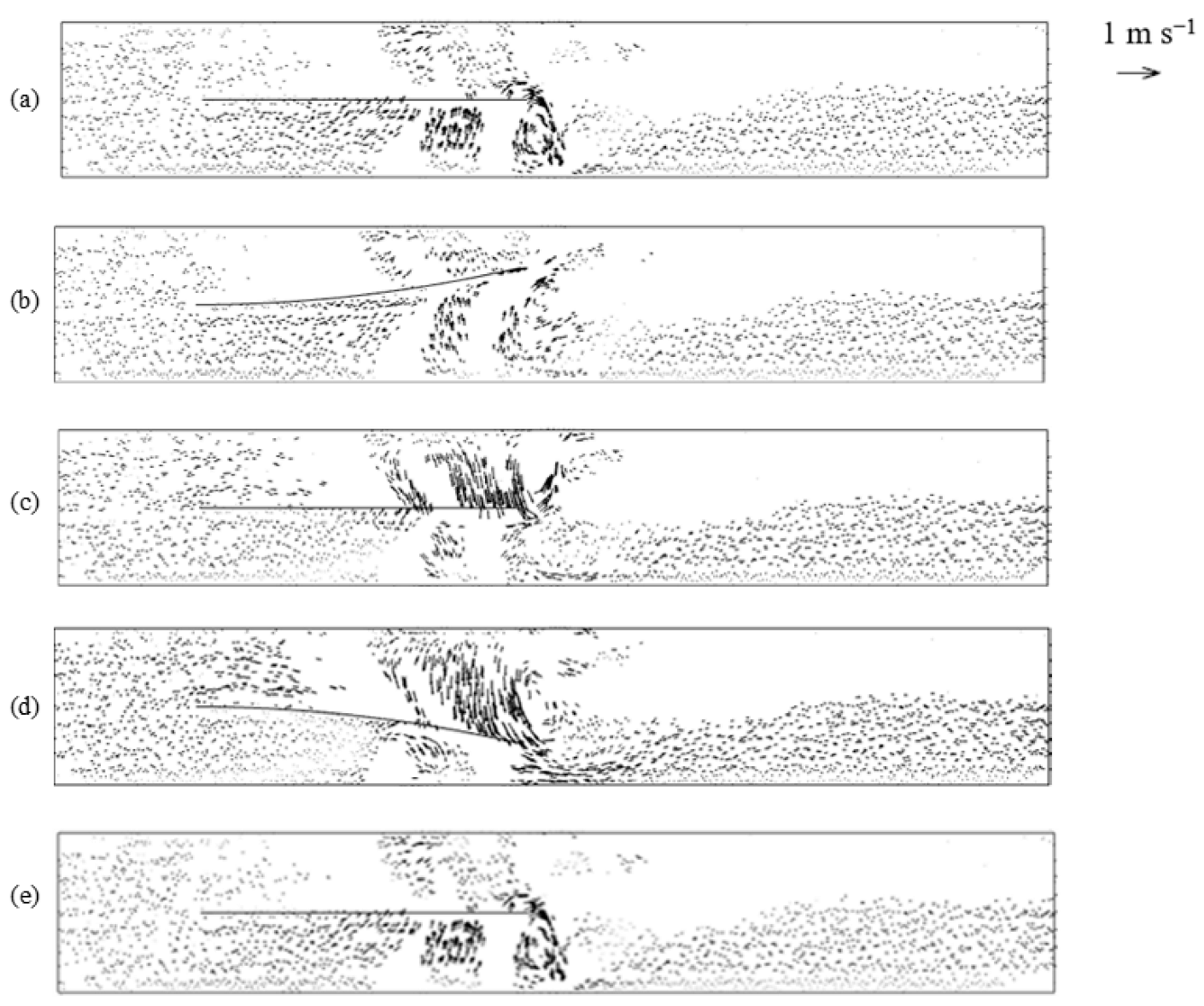
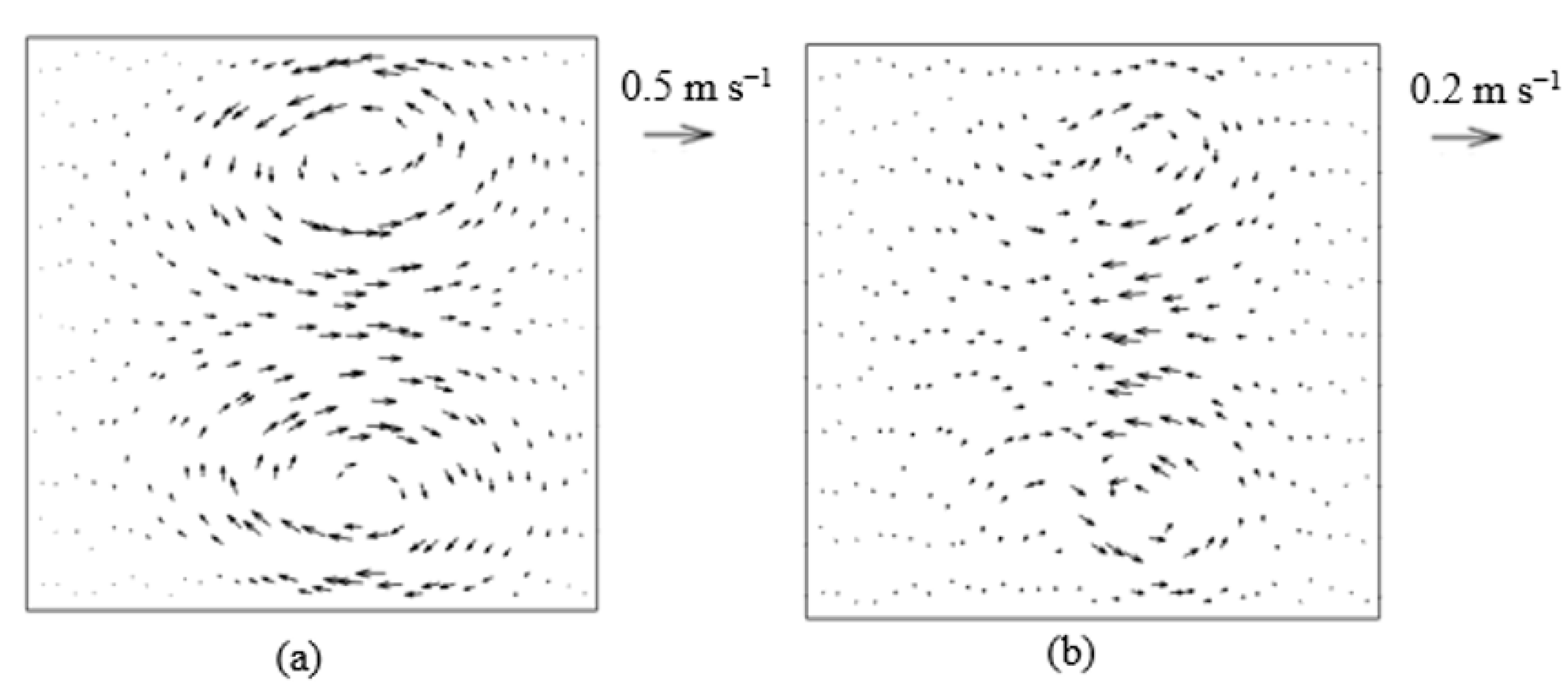
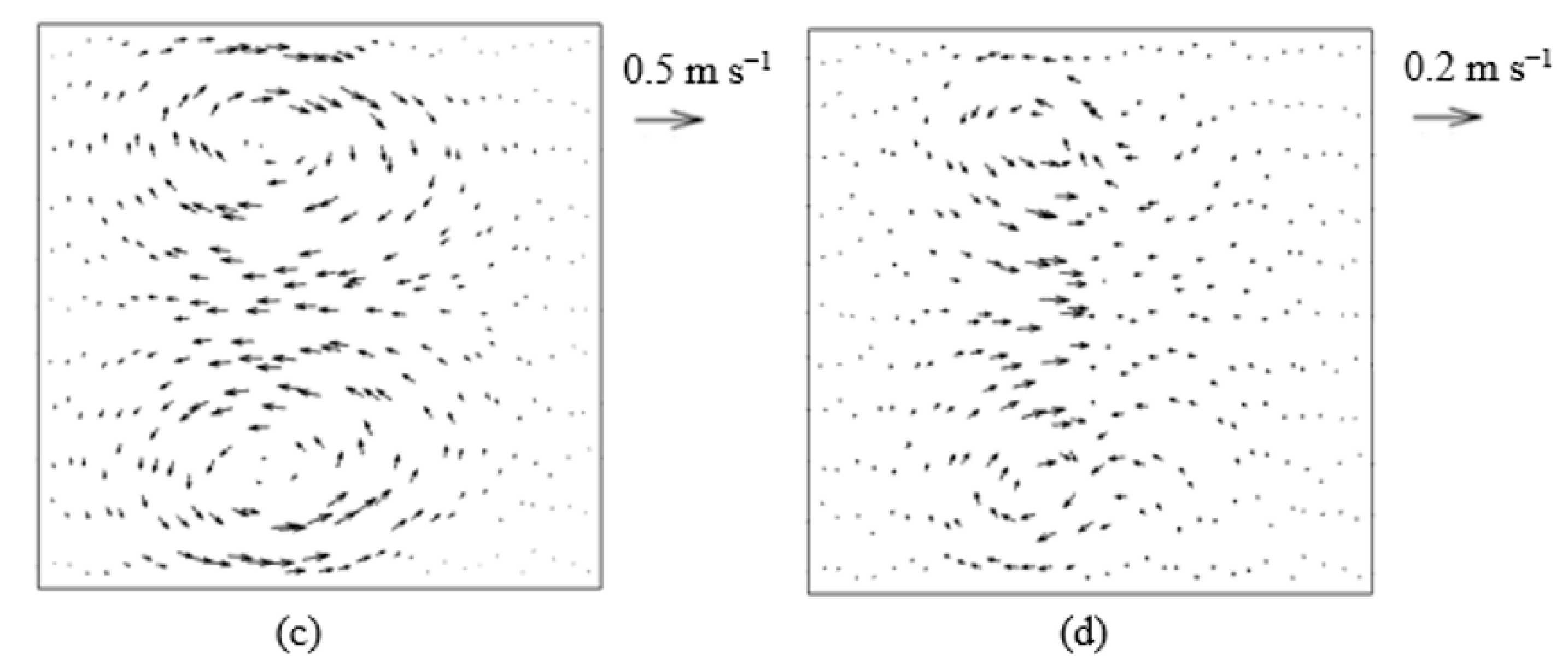
  • The vibrating blade forms the longitudinal vortices. Hence, the heat transfer is enhanced.
  • More than four incommensurable frequencies are in the power spectrum, indicating that the system has reached a chaotic state. The system reaches a chaotic state when the vibrating frequency is over 5 Hz.
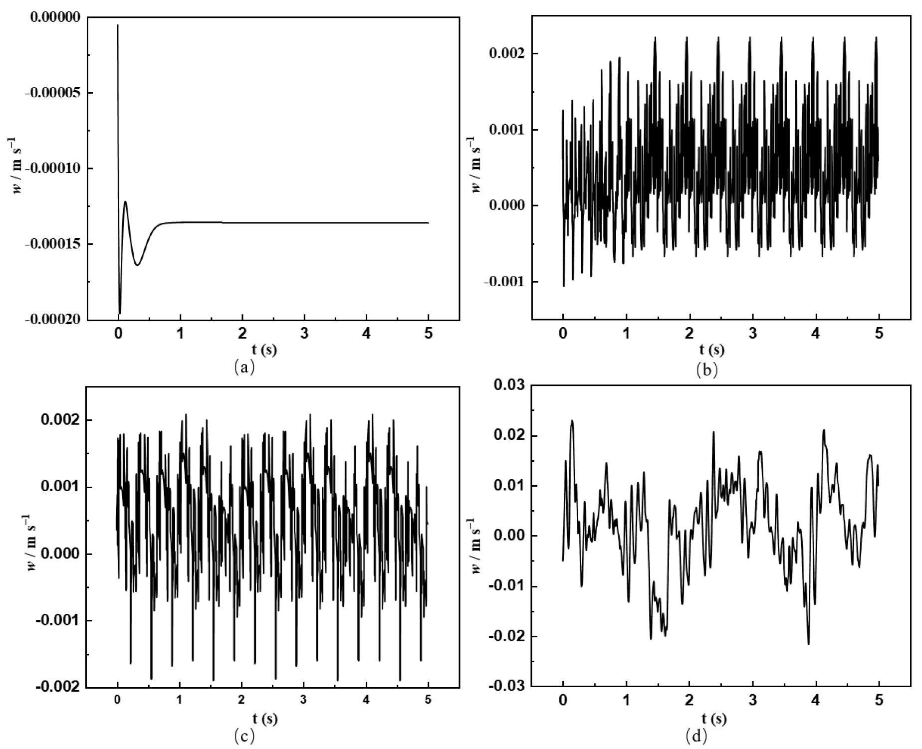
  • As the amplitude increases, the system gradually changes from a steady state to a weakly chaotic one. The amplitude increases further to a periodic state and finally to a chaotic state. The degree of chaos becomes more intense when the amplitude is 8 mm.

Author Contributions

Software, X.Y.; Validation, C.L.; Writing—original draft, X.Y.; Writing—review & editing, J.H., Y.F. and C.M. All authors have read and agreed to the published version of the manuscript.

Funding

The present work was financially supported by the National Natural Science Foundation of China (No. 52276059), the Natural Science Foundation of Tianjin in China (20JCZDJC00470), and the Key Training Fund for “Project & Team” of Tianjin in China (No. XC202042).

Conflicts of Interest

The authors declare that they have no known competing financial interests or personal relationships that could have appeared to influence the work reported in this paper.

Abbreviations

Nomenclature
Aamplitude, mm
cpspecific heat of air, J kg−1 K−1
Dadimensionless amplitude
Dhthe equivalent diameter, mm
ffrequency, Hz
kthermal conductivity, W m−2 K−1
llength of the blade, mm
mmass, kg
hconvective heat transfer coefficient, W m−2 K−1
havaverage convective heat transfer coefficient, W m−2 K−1
ppressure, Pa
qthe heat flow density
Ttemperature, K
vininlet velocity, m s −1
uvelocity in x-direction, m s −1
Vvolume
vvelocity in the y-direction, m s −1
wvelocity in the z-direction, m s −1
Greek symbols
Γdiffusion coefficient
λthermal conductivity, Wm−1 K−1
ρfluid density, kg m−3
τdelay time, s
μthe dynamic viscosity, kg m−1 s−1
Dimensionless groups
NuNusselt number
PrPrandtl number
ReReynolds number
MLEMaximum Lyapunov exponent
Subscript
aair
avaverage value
bladevibrating blade
maxmaximum value

References

  1. Aref, H. The development of chaotic advection. Phys. Fluids 2002, 14, 1315–1325. [Google Scholar] [CrossRef]
  2. Bueghelea, T.; Segre, E. Chaotic flow and efficient mixing in a microchannel with a polymer solution. Phys. Rev. E 2004, 69, 066305. [Google Scholar] [CrossRef] [PubMed] [Green Version]
  3. Tripathi, E.; Patowari, P.K.; Pati, S. Numerical investigation of mixing performance in spiral micromixers based on Dean flows and chaotic advection. Chem. Eng. Process. 2021, 169, 108609. [Google Scholar] [CrossRef]
  4. Karami, M.; Shirani, E.; Jarrahi, M.; Peerhossaini, H. Mixing by time-dependent orbits in spatiotemporal chaotic advection. J. Fluids Eng. 2015, 137, 011201. [Google Scholar] [CrossRef]
  5. Jarrahi, M.; Castelain, C.; Peerhossaini, H. Mixing enhancement by pulsating chaotic advection. Chem. Eng. Process. 2013, 74, 1–13. [Google Scholar] [CrossRef]
  6. Boyland, P.L.; Aref, H.; Stremler, M.A. Topological fluid mechanics of stirring. J. Fluid Mech. 2000, 403, 277–304. [Google Scholar] [CrossRef] [Green Version]
  7. Balachandar, S. Chaotic Advection in Stokes Flow. Phys. Fluids 1986, 29, 3515. [Google Scholar]
  8. Gepner, S.W.; Floryan, J.M. Use of Surface corrugations for Energy-Efficient Chaotic Stirring in Low Reynolds number flows. Sci. Rep. 2020, 10, 9865. [Google Scholar] [CrossRef]
  9. Yada, N.; Kundu, P.; Paul, S.; Pal, P. Different routes to chaos in low Prandtl-number Rayleigh–Bénard convection. Int. J. Non-Linear Mech. 2016, 81, 261–267. [Google Scholar] [CrossRef]
  10. Cimarelli, A.; Angeli, D. Routes to chaos of natural convection flows in vertical channels. Int. Commun. Heat Mass Transf. 2017, 81, 201–209. [Google Scholar] [CrossRef]
  11. Bhowmick, S. Transition to a chaotic flow in a V-shaped triangular cavity heated from below. Int. J. Heat Mass Transf. 2019, 128, 76–86. [Google Scholar] [CrossRef]
  12. Brett, G.J.; Pratt, L.; Rypina, I. Competition between chaotic advection and diffusion: Stirring and mixing in a 3-D eddy model. Nonlinear Process. Geophys. 2019, 26, 37–60. [Google Scholar] [CrossRef] [Green Version]
  13. Oteski, L.; Duguet, Y.; Pastur, L.; Quéré, P.L. Quasiperiodic routes to chaos in confined two-dimensional differential convection. Phys. Rev. E 2015, 92, 043020. [Google Scholar] [CrossRef] [Green Version]
  14. Gao, Z.; Sergent, A.; Podvin, B.; Xin, S.; Quéré, P.L.; Tuckerman, L.S. Transition to chaos of natural convection between two infinite differentially heated vertical plates. Phys. Rev. E 2013, 88, 023010. [Google Scholar] [CrossRef] [Green Version]
  15. Li, K.; Xun, B.; Hu, W.R. Some bifurcation routes to chaos of thermocapillary convection in two-dimensional liquid layers of finite extent. Phys. Fluids 2016, 28, 130. [Google Scholar] [CrossRef] [Green Version]
  16. Pouryoussefi, S.M.; Zhang, Y. Analysis of chaotic flow in a 2D multi-turn closed-loop pulsating heat pipe. Appl. Therm. Eng. 2017, 126, 1069–1076. [Google Scholar] [CrossRef] [Green Version]
  17. Pouryoussefi, S.M. Numerical investigation of chaotic flow in a 2D closed-loop pulsating heat pipe. Appl. Therm. Eng. 2016, 98, 617–627. [Google Scholar] [CrossRef]
  18. Ghaedamini, H.; Lee, P.S.; Teo, C.J. Enhanced transport phenomenon in small scales using chaotic advection near resonance. Int. J. Heat Mass Transf. 2014, 77, 802–808. [Google Scholar] [CrossRef]
  19. Cheng, S.; Zhou, T.; Li, J.J. Nonlinear Analysis of Natural Circulation Critical Heat Flux in Narrow Channels. At. Energy Sci. Technol. 2012, 46, 1330–1335. [Google Scholar]
  20. Bahiraei, M.; Mazaheri, N.; Alighardashi, M. Development of chaotic advection in laminar flow of a non-Newtonian nanofluid: A novel application for efficient use of energy. Appl. Therm. Eng. 2017, 124, 1213–1223. [Google Scholar] [CrossRef]
  21. Guzman, A.M.; Amon, C.H. Transition to chaos in converging-diverging channel flows: Ruelle-Takens-Newhouse scenario. Phys. Fluids 1994, 6, 1994–2002. [Google Scholar] [CrossRef]
  22. Cristina, H.; Amon, C.H.; Morel, B. Lagrangian chaos, Eulerian chaos, and mixing enhancement in converging–diverging channel flows. Phys. Fluids 1996, 8, 1192–1206. [Google Scholar]
  23. Kang, Q.; Jiang, H.; Duan, L.; Zhang, C.; Hu, W. The critical condition and oscillation-transition characteristics of thermocapil-lary convection in the space experiment on SJ-10 satellite. Int. J. Heat Mass Transf. 2019, 135, 479–490. [Google Scholar] [CrossRef] [Green Version]
  24. Tohidi, A.; Shokrpour, M.; Hosseinalipour, S.M. Heat transfer enhancement utilizing chaotic advection in coiled tube heat exchangers. Appl. Therm. Eng. 2015, 76, 185–195. [Google Scholar] [CrossRef]
  25. Tohidi, A.; Ghaffari, H.; Nasibi, H.; Mujumdar, A.S. Heat transfer enhancement by combination of chaotic advection and nanofluids flow in helically coiled tube. Appl. Therm. Eng. 2015, 86, 91–105. [Google Scholar] [CrossRef] [Green Version]
  26. Leonard, A. Large-eddy simulation of chaotic convection and beyond. In Proceedings of the 35th Aerospace Sciences Meeting and Exhibit, Reno, NV, USA, 6–9 January 1997. [Google Scholar]
  27. Siddiqa, S.; Naqvi, S.B.; Azam, M.; Aly, A.M.; Molla, M.M. Large-eddy-simulation of turbulent buoyant flow and conjugate heat transfer in a cubic cavity with fin ribbed radiators. Numer. Heat Transf. 2023, 83, 900–918. [Google Scholar] [CrossRef]
  28. Song, Y.; Xu, J. Chaotic behavior of pulsating heat pipes. Int. J. Heat Mass Transf. 2009, 52, 2932–2941. [Google Scholar] [CrossRef]
  29. Jian, Q.; Wu, H.; Ping, C. Non-linear analyses of temperature oscillations in a closed-loop pulsating heat pipe. Int. J. Heat Mass Transf. 2009, 52, 3481–3489. [Google Scholar]
  30. Chen, C.W.; Li, F.; Wang, X.Y.; Zhang, G.M. Improvement of flow and heat transfer performance of manifold microchannel with porous fins. Appl. Therm. Eng. 2022, 206, 118129. [Google Scholar] [CrossRef]
  31. Jou, R.; Tzeng, S. Numerical research of nature convective heat transfer enhancement filled with nanofluids in rectangular enclosures. Int. Commun. Heat Mass Transf. 2006, 33, 727–736. [Google Scholar] [CrossRef]
  32. Liu, S.F.; Huang, R.T.; Sheu, W.J. Heat transfer by a piezoelectric fan on a flat surface subject to the influence of horizontal/vertical arrangement. Int. J. Heat Mass Transf. 2009, 52, 2565–2570. [Google Scholar] [CrossRef]
  33. Lin, C.N. Enhanced heat transfer performance of cylindrical surface by piezoelectric fan under forced convection conditions. Int. J. Heat Mass Transf. 2013, 60, 296–308. [Google Scholar] [CrossRef]
  34. Shyu, J.C.; Shyu, J.Z. Investigation of heat transfer enhancement of vertical heat sinks by piezoelectric fan. In Proceedings of the 2011 6th International Microsystems, Packaging, Assembly and Circuits Technology Conference (IMPACT), Taipei, Taiwan, 19–21 October 2011; pp. 466–469. [Google Scholar]
  35. Ding, P.; Liu, Z. Study on the Convective Heat Transfer Characteristic of a Horizontal Piezoelectric Fan. J. Phys. Conf. Ser. 2020, 1670, 012013. [Google Scholar] [CrossRef]
  36. Lin, C.N. Heat transfer enhancement analysis of a cylindrical surface by a piezoelectric fan. Appl. Therm. Eng. 2013, 50, 693–703. [Google Scholar] [CrossRef]
  37. Lin, C.N.; Leu, J.S. Analysis of Heat Transfer and Flow Characteristics for the Arrangement of piezoeletric fan on heated cylinder. Heat Tran. Eng. 2015, 36, 1525–1539. [Google Scholar] [CrossRef]
  38. Lin, C.N.; Leu, J.S. Study of thermal and flow characteristics of a heated cylinder under dual piezoelectric fans actuation. Int. J. Heat Mass Transf. 2014, 78, 1008–1022. [Google Scholar] [CrossRef]
  39. Tan, L.; Zhang, J.Z.; Tan, X.M. Numerical investigation of convective heat transfer on a vertical surface due to resonating cantilever beam. Int. J. Therm. Sci. 2014, 80, 93–107. [Google Scholar]
  40. Lin, C.N. Analysis of three-dimensional heat and fluid flow induced by piezoelectric fan. Int. J. Heat Mass Transf. 2012, 55, 3043–3053. [Google Scholar] [CrossRef]
  41. Kim, K.; Yeom, T. Numerical study on channel-flow convection heat transfer enhancement with piezoelectric fans under various operating conditions. Appl. Therm. Eng. 2023, 219, 119674. [Google Scholar] [CrossRef]
  42. Choi, M.; Cierpka, C.; Kim, Y.H. Vortex formation by a vibrating cantilever. J. Fluids Struct. 2012, 31, 67–78. [Google Scholar] [CrossRef]
  43. Sufian, S.F.; Abdullah, M.Z.; Mohamed, J.J. Effect of synchronized piezoelectric fans on microelectronic cooling performance. Int. Commun. Heat Mass Transf. 2013, 43, 1–89. [Google Scholar] [CrossRef]
  44. Sufian, S.F.; Fairuz, Z.M.; Zubair, M. Thermal analysis of dual piezoelectric fans for cooling multi-LED packages. Microelectron. Reliab. 2014, 54, 1534–1543. [Google Scholar] [CrossRef]
  45. Hu, J.Q.; Wang, K.; Xie, L.Y.; Min, C.H.; Rao, Z.H. Effects of electromagnetic-vibration fan with folding blades on convective heat transfer. Appl. Therm. Eng. 2022, 213, 118651. [Google Scholar] [CrossRef]
  46. Soong, C.Y.; Huang, W.T. Triggering and enhancing chaos with a prescribed target Lyapunov exponent using optimized perturbations of minimum power. Phys. Rev. E 2007, 75, 036206. [Google Scholar] [CrossRef] [PubMed]
  47. Kennel, M.B.; Brown, R.; Abarbanel, H. Determining embedding dimension for phase-space reconstruction using a geometrical construction. Phys. Rev. A 1992, 45, 3403–3411. [Google Scholar] [CrossRef] [PubMed] [Green Version]
  48. Tiwari, J.; Yeom, T. Enhancement of channel-flow convection heat transfer using piezoelectric fans. Appl. Therm. Eng. 2021, 191, 113917. [Google Scholar] [CrossRef]
  49. Fallenius, B.; Sattari, A.; Fransson, J. Experimental study on the effect of pulsating inflow to an enclosure for improved mixing. Int. J. Heat Fluid Flow 2013, 44, 108–119. [Google Scholar] [CrossRef]
  50. Hideshi, I. The second largest Lyapunov exponent and transition to chaos of natural convection in a rectangular cavity. Int. J. Heat Mass Transf. 2006, 49, 5035–5048. [Google Scholar]
  51. Speetjens, M.; Metcalfe, G.; Rudman, M. Lagrangian transport and chaotic advection in three dimensional laminar flows. Appl. Mech. Rev. 2021, 73, 030801. [Google Scholar] [CrossRef]
  52. Anxionnaz, Z.; Minvielle, P.T.; Couturier, R. Implementation of ‘chaotic’ advection for viscous fluids in heat exchanger/reactors. Chem. Eng. Process. 2017, 113, 118–127. [Google Scholar] [CrossRef] [Green Version]
Figure 1. Computational domain.
Energies 16 03076 g001
Figure 2. Computational domain grid diagram.
Energies 16 03076 g002
Figure 3. Grid independence validation.
Energies 16 03076 g003
Figure 4. Model validation. Numerical results compared with the experimental results of research [48].
Energies 16 03076 g004
Figure 5. The effects of the natural frequency and the amplitude of the blade on the heat transfer performance: (a) frequency at A = 5 mm; (b) amplitude at f = 5 Hz.
Energies 16 03076 g005
Figure 6. Relationship between Nu and Reynolds numbers.
Energies 16 03076 g006
Figure 7. Temperature contour of the heated surface: (a) without blade; (b) Phase 0π; (c) Phase π/2.
Energies 16 03076 g007
Figure 8. Velocity vector at different phases of z = 0 mm: (a) Phase 0π; (b) Phase π/2; (c) Phase π; (d) Phase 3π/2; (e) Phase 2π.
Energies 16 03076 g008
Figure 9. Velocity vectors at y = 50 mm: (a) Phase π/2; (b) Phase π; (c) Phase 3π/2; (d) Phase 2π.
Energies 16 03076 g009aEnergies 16 03076 g009b
Figure 10. Schematic view of the Poincaré map.
Energies 16 03076 g010
Figure 11. Poincaré map for different frequencies: (a) without blade; (b) f = 5 Hz; (c) f = 10 Hz.
Energies 16 03076 g011
Figure 12. The partial velocity w against time: (a) f = 1 Hz; (b) f = 3 Hz; (c) f = 5 Hz; (d) f = 10 Hz.
Energies 16 03076 g012
Figure 13. Variation of power spectral density: (a) f = 1 Hz; (b) f = 3 Hz; (c) f = 5 Hz; (d) f = 10 Hz.
Energies 16 03076 g013
Figure 14. Phase space trajectories for different amplitudes.
Energies 16 03076 g014
Figure 15. Phase space trajectories for A = 4 mm: (a) point 1; (b) point 2; (c) point 3; (d) point 4.
Energies 16 03076 g015
Figure 16. Phase space trajectories for A = 8 mm: (a) point 1; (b) point 2; (c) point 3; (d) point 4.
Energies 16 03076 g016
Figure 17. Determination of the delay time.
Energies 16 03076 g017
Figure 18. Associated dimensions.
Energies 16 03076 g018
Figure 19. Maximum Lyapunov exponent.
Energies 16 03076 g019
Disclaimer/Publisher’s Note: The statements, opinions and data contained in all publications are solely those of the individual author(s) and contributor(s) and not of MDPI and/or the editor(s). MDPI and/or the editor(s) disclaim responsibility for any injury to people or property resulting from any ideas, methods, instructions or products referred to in the content.

