Analysing Grid-Level Effects of Photovoltaic Self-Consumption Using a Stochastic Bottom-up Model of Prosumer Systems ^†

Abstract

Self-consumption of the energy generated by photovoltaics (PV) is playing an increasingly important role in the power grid. “Prosumer” systems consume part of the produced energy directly to meet the local demand, which reduces the feed-in into as well as the demand from the grid. In order to analyse the effects of PV self-consumption in the power grid, we introduce a stochastic bottom-up model of PV power generation and local consumption in the control area of the German transmission system operator TransnetBW. We set up a realistic portfolio of more than 100,000 PV/prosumer systems to generate representative time series of PV generation and consumption as a basis to derive self-consumption and feed-in. This model allows for the investigation of the time-dependent behaviour in detail for the full portfolio whereas measurements are presently only available as aggregated feed-in time series over a nonrepresentative subset of systems. We analyse the variation of self-consumption with PV generation and consumption at the portfolio level and its seasonal, weekly and diurnal cycles. Furthermore, we study a scenario of 100% prosumers as a limiting case for a situation without subsidized feed-in tariffs and local energy storage.

1. Introduction

The successful integration of a rising share of decentralized electricity generation into the power grid is crucial for the transition to a sustainable energy system. Grid operators find themselves faced with an increase of power generation from fluctuating renewable energy sources accompanied by diversifying strategies of local consumption, short-term storage and marketing of the generated energy. Therefore, reliable information and models for the present and for the forecasting of renewable energy feed-in is becoming increasingly more important for a secure and cost-efficient electricity supply. This study builds on data records and regulatory aspects for Germany, but the problem setting and, hence, the findings can be applied generally to any system with decentralized generation and consumption. Parts of this paper were presented at the 11th Solar & Storage Integration Workshop and published in the workshop’s proceedings [1].

The generation of electric power by photovoltaics (PV) is primarily determined by the incoming solar irradiance. Models to describe its changes with fluctuating weather conditions and solar position have been developed in solar energy meteorology [2]. The local demand has to be considered additionally in order to describe the electricity feed-in since many PV systems are part of an environment of electricity consumers, e.g., a commercial or residential building. These so-called “prosumer” systems simultaneously act as energy producers and consumers in the power grid. Instead of feeding all the generated electricity into the grid, energy can be used for self-consumption, i.e., to meet the local demand directly. The problem of a rising share of prosumers in the power system and its influence on PV feed-in and consumption profiles was discussed in detail in a recent review article [3]. The effect is also called “behind-the-meter PV”, as the balancing between power generation and load in many cases takes place before the measurement point and can therefore not be monitored by utilities or grid operators.

The energy consumption in a power grid is commonly estimated using standard load profiles, in Germany for consumers with an annual demand up to 100 MWh, while the PV feed-in is typically assessed independently [4]. PV self-consumption changes load profiles considerably, which has prompted the idea of developing additional prosumer load profiles [5]. The share of self-consumption in the total energy generated by PV has increased continuously over the past years, reaching around 7% in Germany in the year 2018 [6]. It can be expected that with decreasing remuneration by feed-in tariffs (FITs) and increasing energy purchase prices, self-consumption will become even more attractive in the very near future [7]. For roof-mounted PV systems in Germany, a growth up to almost 15% in 2025 was predicted [8]. With a targeted development in total installed nominal PV power from 66.5 GW_p in 2022 to 215 GW_p in 2030 and to 400 GW_p in 2040 in Germany [9], large amounts of self-consumed energy in absolute numbers are anticipated. Hence, errors in the estimation of self-consumption have the potential for disruptive effects on the grid.

Detailed information concerning energy generation, consumption and feed-in on various aggregation levels in the power grid is required for the trading and billing of balancing groups, grid load calculations and operational planning. The decision-making involved is especially challenged by the distributed energy generation and self-consumption [10]. Moreover, in order to accomplish these tasks, grid operators have only limited access to relevant measurement data. Feed-in time series are measured for a subset of PV systems, called “SOL systems” here according to the German accounting category for this class of systems. Generally, these are installations with higher-than-average nominal power, e.g., on commercial or industrial buildings, and it is expected that the profiles cannot simply be extrapolated to the full portfolio of PV systems. Furthermore, transmission system operators (TSOs) can access this data only in terms of transfer time series which are aggregated over entire distribution grids. Time-resolved measurements of PV generation or self-consumption are usually not available at all. The total energy generated by an individual PV system, together with a breakdown into self-consumption and feed-in, can be obtained from annual meter readings. However, this information is known to be incomplete. In Germany, for example, no separate measurements are required for PV systems with a nominal power less than 10 kW_p [6].

The fundamentally different time courses and local balancing of PV generation and electricity consumption build up a complex system. Independent averaging of generation and consumption at the grid level, e.g., using standard load profiles, will not adequately describe actual feed-in and consumption. Instead, an integrated analysis of both is required in order to understand the behaviour of the system as a whole. Since very little measurement data are available for this task, a detailed bottom-up simulation model comprising PV power generation and consumption on an individual prosumer level is chosen here to fill this gap. The approach facilitates a detailed analysis of influencing factors on PV self-consumption and the identification of suitable parameters in data-driven models as a basis to improve PV upscaling methods. It furthermore allows for the estimation of the future effects of expected changes and variable compositions of different prosumer systems in large portfolios. In order to keep the complexity of different usage strategies out, additional technologies such as local battery storages, heat pumps or electric cars are not included in the model at this stage.

In contrast to other approaches of modelling PV self-consumption, the bottom-up simulation allows for the reproduction of the local balancing of PV generation and consumption at the individual prosumer level. In this way, the observed mismatch between PV generation estimates (obtained, e.g., from PV power upscaling) and actually measured feed-in can be described realistically. In a top-down model, this mismatch has to be estimated from an overall perspective on the grid for which currently a good data basis is missing, as the balancing takes place “behind-the-meter” [11]. The results obtained with the stochastic bottom-up model accounting for all individual prosumer systems in a portfolio are thought to better reflect the effects and be suitable to building a basis for the implementation of data-driven models describing the grid-level effects of PV self-consumption. Such a model could follow a top-down approach enriched by other influencing factors, such as the seasonal cycles identified in the bottom-up model.

Other perspectives on PV self-consumption require different modelling approaches. As the model presented here does not cover energy storage, demand-side management or other flexibility options, it cannot describe, for instance, the economics of different prosumer usage strategies. For this, models of single PV prosumers with battery storage under different optimization targets, such as self-sufficiency vs. cost-efficiency maximization, have been examined [12], for example. Energy system optimization models (ESOMs) are used to find globally optimized grid configurations from a top-down perspective [13]. Agent-based models (ABMs), on the other hand, can capture the effects of locally optimized usage strategies of PV prosumers in a grid [14]. The coupling of ESOMs and ABMs has been proposed to study the economics of prosumer business models, regulatory frameworks and cost-efficient energy system design [15]. For the disaggregation of PV generation and consumption profiles from net demand measurements, methods from game theory have also been employed [16].

Our novel approach to PV self-consumption modelling and analysis at the portfolio level is as follows. Based on currently available data records on PV generation, consumption and feed-in and the characteristics of PV systems and prosumers (Section 2.1), we developed a realistic bottom-up simulation model system of self-consumption in the control area of the German TSO TransnetBW (Section 2.2). We validated the prosumer model against available measurement data and quantified the improvement over a linear reference model (Section 3). We analysed the overall effect of self-consumption and its change with yearly, weekly and daily cycles as well as other parameters (Section 4). Furthermore, the expected differences in behaviour in a 100% prosumers scenario were estimated. In the final section of this paper, we conclude with a short summary and outlook (Section 5).

2. Methodology

2.1. Data Sets

Several data sets of PV/prosumer system characteristics and measurements have been used to determine the necessary modelling parameters and for validation. All measurement data used here cover the control area of the German TSO TransnetBW for the full year of 2018 which we used as the modelling period throughout this study.

• PV system master data: All renewable energy systems in remuneration under the German Renewable Energy Sources Act (“Erneuerbare-Energien-Gesetz” EEG) are listed in the EEG master data record. It comprises basic system characteristics such as the nominal power, the date of commissioning, the address and whether time-resolved feed-in measurements are taken. In order to cover the state of the PV portfolio in 2018, the record used here is the version of 18 December 2018. From 31 January 2019 on, the EEG master data was integrated into the Marktstammdatenregister (MaStR) [17], including additional information, e.g., on building usage, which has been used to set-up the prosumer model here.
• Annual meter readings: Regular power meter readings provide annual energy totals for each PV system. The total energy generation is additionally broken down into feed-in under the EEG FIT, self-consumption and direct marketing.
• Transfer time series EUZ: Feed-in time series are recorded on a distribution grid level for the data transfer between the distribution system operator (DSO) and the TSO (in German “Einspeiseüberführungszeitreihen” EUZ). They contain the time course of the PV feed-in under the EEG FIT in a 15 min resolution. For each distribution grid, two time series subsume the “SOL systems” which are measured on the one hand and the “SOT systems” which are derived from estimated feed-in profiles on the other hand. As the latter are not based on measurements, they were not be used in this study.

2.2. Model System

Based on the PV system master data, a stochastic bottom-up model for PV self-consumption building on the combination of existing approaches to describe PV generation and electricity consumption has been developed. This section describes the modelling steps comprising metadata enrichment, PV generation and consumption simulations as well as their aggregation to self-consumption and feed-in in a portfolio.

As the available metadata neither provide full technical information on each PV system nor the details of individual building usages, this missing data are modelled stochastically. It should be emphasised here that although statistically representative ensembles of PV/prosumer systems—and, hence, time series—are generated with this stochastic approach, substantial deviations from the actual power generation and consumption at the individual systems are likely to be observed. However, in aggregating over a sufficiently large portfolio, e.g., at the distribution grid level, a realistic description of the actual power time series can be expected.

2.2.1. System Locations and Building Classification

Knowledge of the location of each PV system is necessary to determine the solar irradiance and to classify the usage category of the local power system into which it is integrated. First, the addresses provided by the system master data have been used for geo-coding, i.e., to determine the geo-coordinates of each system, by an address search in the OpenStreetMap database [18]. For the solar irradiance modelling with satellite data, approximate locations based on incomplete addresses (up to the street name or even postal code level) are usually sufficient to acquire reasonable results. For 329,494 PV systems, such approximate locations were determined and included in the PV generation model. For the consumption modelling, on the other hand, a precise building to which a PV system is attached to has to be identified in order to determine its usage category. As a full address (including the house number) is provided in the system master data for only 119,152 PV systems in the whole control area, the consumption model was restricted to this subset.

For the different consumers, we distinguish three main categories: ground-mounted PV systems (without consumption), residential buildings and commercial buildings. The MaStR record [17] provides a rough classification of building usage for about 25% of the selected PV systems. Further information was retrieved from OpenStreetMap and other publicly available databases. Since for some categories like transportation, no reasonable consumption profiles could be generated with our tools, these buildings were also removed from consideration. Altogether 118,650 out of the 329,510 PV systems could be assigned to a usage category and, hence, were included in the model. These contain 96 ground-mounted systems, 98,066 residential buildings and 20,488 nonresidential buildings.

2.2.2. Generation Model

In this section, the PV generation model is briefly summarized. A more detailed description was published earlier [19]. The modelling of PV generation is based on PV power simulations with the software ZENIT [20] and requires solar irradiance and ambient temperature as input as well as information on technical and environmental PV system parameters.

Solar Irradiance and Temperature

Irradiances are calculated from meteorological satellite image data using the Heliosat method [21]. Images are provided by EUMETSAT Meteosat Second Generation (MSG) satellites in a temporal resolution of 15 min. The high-resolution visible (HRV) broadband channel is used as input to calculate 15 min averages of the global horizontal irradiance ($\mathrm{GHI}$) for the entire control area of TransnetBW in a spatial resolution of approximately 1.3 km × 2.2 km. The irradiance on the tilted PV modules is derived by splitting the $\mathrm{GHI}$ into its diffuse and direct components using the DIRINT model [22] followed by a transposition to plane-of-array irradiance [23]. Ambient temperatures are extracted from high-resolution deterministic weather forecasts by the European Centre for Medium-Range Weather Forecasts (ECMWF).

PV System Classification and Simulation Parameters

The system parameters for the PV simulation are chosen based on the information provided by the PV system master data record. To this end, the systems are classified into 5 nominal power categories with limits of 10, 30, 100 and 1000 kW_p and two age categories by date of commissioning before and after 1 January 2010. For the resulting 10 classes of systems, assumptions on the system environment and technologies are made based on long-standing experience with yield assessments and monitoring of PV systems. An overview of the different PV simulation parameters is given in

Table 1. Technical and environmental parameters used for the PV power simulation with the range of values for the different classes of PV systems.

Ambient temperature increase in settlements	up to 5 K
Irradiance-induced module temperature increase	25–35 K at 1000 W/m2
Mean shading horizons	at 3°–7° solar elevation
Internal shading losses	1–2% for systems above 100 kWp
Degradation losses	0.25% per year of operation
String, medium, central inverters	typical models built in 2005/2015
Medium-voltage transformers	for systems above 100 kWp

.

PV Module Orientations

The module orientation is particularly important for a realistic modelling of PV generation. To achieve a realistic representation, a stochastic method based on reference data from real PV systems is deployed here. Typical orientations of PV systems in Germany were investigated in various studies [24,25]. The classification into the above-mentioned nominal power categories reflects typical installation surfaces (pitched roofs, flat roofs, ground) and, thus, the constraints for module orientations [26]. A reference data set of about 35,000 PV systems in Germany is used here for orientation modelling, including information on location, orientation and nominal power [25]. In a stochastic attribution, to each PV system in the simulation the orientation angles of a randomly chosen system in the same nominal power category from the reference data set are assigned. In this way, the joint distribution of both angles is reproduced. For the 212 PV systems with a nominal power above 1 MW_p only very few reference systems are available. As the contribution of those systems to the total PV power generation is particularly large, the orientation was determined manually on the basis of satellite images when possible. Tilt and azimuth angles that could not be determined in this way are then drawn independently from known distributions [26]. Figure 1 shows the marginal distributions of both angles for all power categories.

Postprocessing to Account for Additional Losses

A realistic representation of a portfolio has to rely on observations of the actual technical and environmental conditions of real PV systems. An intrinsic problem rises from the fact that these conditions are examined only for PV systems subject to quality monitoring which, consequently, results in higher-than-average performance. The causes of lower performance in the vast majority of PV systems are known: extensive shading, soiling, technical defects and other types of losses. All of these can, in principle, be modelled precisely, but representative measurements to calibrate to are inherently missing. For this reason, additional losses are described here with a linear scaling based on the distribution of measured specific yields (energy totals per nominal power). For each system, the simulated PV output power is scaled by an individual factor such that in each class, the spread of the simulated specific yields matches the corresponding spread in the annual meter readings data set. All PV generation time series are sampled down to the hourly resolution of the consumption model described in the following section.

2.2.3. Consumption Model

As consumption profiles strongly depend on the usage categories, the modelling steps here are completely different for residential and nonresidential buildings.

Residential Sector

The software synPRO [27] is used to generate synthetic load profiles for residential buildings. It employs a stochastic bottom-up approach of simulating the consumption on a device level and subsequent aggregation. For each dwelling, the number of inhabitants is estimated from the building area in OpenStreetMap and a socioeconomic status is assigned according to the distribution in the Zensus 2011 data [28]. A stock of devices is selected matching the inhabitants and their socioeconomic status. For each device, a load profile is generated depending on the type of device as well as the intensity and duration of usage. The underlying probabilities are derived from HETUS [29]. By summation over all devices, electrical load profiles are created for 420 different configurations of households.

Nonresidential Sector

For nonresidential buildings, a simulation tool developed in the project synGHD [30] is used to model consumption. In this project, energy consumption in the sectors commerce, trade and service was investigated. LSTM (long short-term memory) neural networks were trained on a data collection of 485 electrical load profiles. These load profiles were further subdivided into 18 usage categories. As features, hour of the day, day of the week, information about holidays and weather information from ERA 5 reanalysis data [31] are chosen. Due to strongly facility-dependent energy consumption in the sectors commerce, trade and service, the results have to be scaled to a realistic annual demand. As industrial energy consumption was not considered in the synGHD project, industry is treated as commerce.

For scaling, typical electricity consumption in the region of interest has to be identified. As the control area of TransnetBW closely matches that of the federal state of Baden–Württemberg, information about the companies has been taken from the official business register of the state office for statistics [32]. This provides the number of companies and the number of employees subjected to social insurance contributions in the individual branches of the economy. From the official energy balance for Baden–Württemberg [33], information about the energy demand in the different categories was derived. Since the energy consumption for the sector commerce, trade and service, the transport sector and the residential sector is only available as aggregate over the respective sector, the energy consumption was split according to typical energy consumption per employee as published by the AG Energiebilanzen [34]. After a scaling to the demand from the official energy balance, this gives an annual average demand per company in the specific economic branch. As electricity consumption in the agricultural sector cannot be derived the way described above, typical demands as published by the Bayerische Landesanstalt für Landwirtschaft [35] are used.

Modelling Consumption

For reasons of computational effort, the consumption time series are generated in an hourly time resolution. The residential sector is modelled by a cluster approach. For the 420 configurations of households, up to 200 load profiles per type are generated. From these clusters, load profiles are drawn randomly. The load profiles for the nonresidential sector are generated for each building individually with the determined usage category and total consumption.

In Figure 2, the mean electric load for the different days of the week in the model are visualized. In the model, nonresidential load is considerably higher than residential load. It exhibits strong differences between workdays and weekends and remains almost at the base level for the whole of Sunday. In contrast, residential buildings have less variation in the course of week, with loads being slightly higher on weekends. The overall load, as a mixture of both, is dominated by the nonresidential part in the morning and by the residential part in the afternoon and evening. On Sundays, the total load basically resembles the residential load in its time course.

2.2.4. Self-Consumption Model

After the simulation of electric power time series of PV generation $P_{\mathrm{PV}}^{\left(i\right)}$ and consumption $P_{\mathrm{Load}}^{\left(i\right)}$ for each prosumer system i, the self-consumption and feed-in time series can be calculated as follows. Without energy storage devices or demand-side management, prosumers do not, in principle, have any abilities to adapt either their electricity generation or consumption. Hence, they are considered as “passive” here using at any time as much as possible of the PV generation power to meet the local demand. Any excess or shortage in the local generation is then balanced via the power grid.

As meeting the local demand is prioritized, the self-consumption $P_{\mathrm{SC}}^{\left(i\right)}$ at any time step is the minimum of current PV generation and consumption,

$$P_{\mathrm{SC}}^{\left(i\right)}=min\left\{P_{\mathrm{PV}}^{\left(i\right)},P_{\mathrm{Load}}^{\left(i\right)}\right\}.$$

(1)

The surplus of the generated power is transferred to the grid as feed-in $P_{\mathrm{FI}}^{\left(i\right)}$,

$$P_{\mathrm{FI}}^{\left(i\right)}=P_{\mathrm{PV}}^{\left(i\right)}-P_{\mathrm{SC}}^{\left(i\right)}=max\left\{P_{\mathrm{PV}}^{\left(i\right)}-P_{\mathrm{Load}}^{\left(i\right)},0\right\}.$$

(2)

For PV systems not acting as prosumers, self-consumption is zero ($P_{\mathrm{SC}}^{\left(i\right)}=0$), and hence, PV generation equals feed-in ($P_{\mathrm{FI}}^{\left(i\right)}=P_{\mathrm{PV}}^{\left(i\right)}$).

Aggregated time series of PV generation, load, feed-in and self-consumption over a portfolio are obtained straightforwardly by summing over all individual systems,

$$P_{\mathrm{PV}}=\sum _i{P}_{\mathrm{PV}}^{\left(i\right)},\mathrm{accordingly}\mathrm{for}{P}_{\mathrm{Load}},P_{\mathrm{FI}},P_{\mathrm{SC}}.$$

(3)

Energy yields over days, months or years are computed as integrals over the respective time interval for all power quantities, $E_{\mathrm{PV}}=\int P_{\mathrm{PV}}\mathrm{d}t$ and accordingly for $E_{\mathrm{Load}}$, $E_{\mathrm{FI}}$, $E_{\mathrm{SC}}$.

For the comparison of portfolios differing in size and composition, a normalization of powers and energy yields by the total nominal PV power $P_{\mathrm{nom}}={\sum }_i{P}_{\mathrm{nom}}^{\left(i\right)}$ in the portfolio is used, giving the specific powers,

$${\widehat{P}}_{\mathrm{PV}}=P_{\mathrm{PV}}/P_{\mathrm{nom}},\mathrm{accordingly}\mathrm{for}{\widehat{P}}_{\mathrm{Load}},{\widehat{P}}_{\mathrm{FI}},{\widehat{P}}_{\mathrm{SC}},$$

(4)

and specific yields ${\widehat{E}}_{\mathrm{PV}}=E_{\mathrm{PV}}/P_{\mathrm{nom}}$, respectively.

Self-consumption rates can then be derived as shares of self-consumption of PV generation on an annual basis or time-resolved as follows:

$$E_{\mathrm{SC}}/E_{\mathrm{PV}}={\widehat{E}}_{\mathrm{SC}}/{\widehat{E}}_{\mathrm{PV}},P_{\mathrm{SC}}/P_{\mathrm{PV}}={\widehat{P}}_{\mathrm{SC}}/{\widehat{P}}_{\mathrm{PV}}.$$

(5)

3. Model Validation

As described in Section 2.1, the measurement data available for a rigorous validation are very limited. We completed two steps of validation, comparing the simulation results first with the annual meter readings and second with the transfer time series EUZ. The different data sets do not provide fully coherent information about which PV systems actually perform self-consumption. Some PV systems do not report any self-consumed energy in the annual meter readings although they are registered as “designed for self-consumption” in the system master data record and vice versa. As the regulations of the German Renewable Energy Act EEG do not require reporting self-consumption for PV systems up to 10 kW_p, this is not necessarily an error in the data. Therefore, the set of prosumers in the model portfolio was selected differently for the two validation steps according to the best information available.

3.1. Comparison with Annual Meter Readings

The structure of the full model portfolio with 118,650 PV systems is presented in

Table 2. Composition of the full model portfolio with the number of PV systems (total nominal power in parentheses) by type of installation and information on self-consumption capability.

	All PV Systems	Systems Designed for Self-Consumption	Systems with Reported Self-Consumption
All installations	118,650 (1755 MWp)	41,033 (566 MWp)	22,705 (405 MWp)
Residential	98,066 (952 MWp)	35,511 (334 MWp)	18,542 (211 MWp)
Nonresidential	20,488 (791 MWp)	5493 (231 MWp)	4148 (193 MWp)
Ground mounted	96 (12 MWp)	29 (1 MWp)	15 (1 MWp)

. For the first step of validation, annual totals of simulated PV generation, feed-in, and self-consumption were compared to the corresponding meter readings which are available for almost 117 thousand PV systems in the portfolio. Here, it is assumed, that only the PV systems with reported self-consumption (Table 2, right column) are prosumers.

Table 3. Comparison of the annual meter readings with the corresponding simulated energy sums. Here, feed-in integrates feed-in both under FIT and for direct marketing. The relative deviation is the difference between simulation and the reading normalized by the reading value.

	Meter Readings	Simulation	Relative Deviation
PV generation	1667 GWh	1725 GWh	+3.5%
Feed-in	1528 GWh	1601 GWh	+4.8%
Self-consumption	139 GWh	124 GWh	−10.7%
Self-consumption rate	8.3%	7.2%	−13.3%

shows the results. The model slightly overestimates the reported annual PV generation (3.5%) but underestimates self-consumption by 10.7%. There are several explanations for this deviation. First, the model does not consider battery storages and load management, which are often designed to increase self-consumption capabilities. Second, especially in the nonresidential case, consumption profiles are very individual and not straightforward to identify. Particularly industry, the sector with the potentially largest consumption, is not considered as a separate usage category. Furthermore, due to data availability, no postprocessing calibration is performed on the consumption model. The resulting modelled self-consumption rate is 7.2%, slightly below the 8.3% from the meter readings. Finally, this results in a deviation of less than 5% of the modelled PV feed-in compared to the meter readings. This is overall an acceptable agreement which indicates that the prosumer model can quantitatively represent different factors contributing to PV power feed-in.

3.2. Comparison with Transfer Time Series

In a second validation step, the time series generated by the prosumer model were compared to the SOL transfer time series EUZ. This represents the part of the PV systems which are measured. Those systems for which the feed-in is estimated based on feed-in profiles by the grid operators (SOT systems) were not considered for validation. It is worth noting at this point that all metadata records and measurements used here were collected under real operating conditions for regulatory and market processes and not to provide an exact basis for scientific evaluations. Furthermore, as described above, our model portfolio does not include all systems. Therefore, a subset of the EUZ time series has to be selected in order to minimize irregularities in and between the different data sets. The validation is in this part restricted to distribution grids for which the following quality criteria apply:

• The difference between the annual feed-in energy integrated over the EUZ and the meter reading sum over all systems is less than 5%.
• The share of systems (in number and nominal power) for which meter readings are available is at least 90%.
• The EUZ contains data for the whole year, and no irregularities like jumps or data gaps are observed.
• There are at least 10 systems of the distribution grid in the model portfolio.
• The model portfolio contains at least 50% of the SOL systems in the distribution grid.

This quality check selects 34 out of the 157 distribution grids for the validation of time series. These 34 distribution grids contain, according to the system master data, 2711 SOL systems with 369.5 MW_p nominal power out of which the prosumer model covers 1761 systems with 225.1 MW_p nominal power.

Table 4. Composition of the SOL systems portfolio for time series validation with the number of PV systems (total nominal power in parentheses) by type of installation and information on self-consumption capability.

	PV Systems	Designed for SC
All installations	1761 (225 MWp)	610 (69 MWp)
Residential	360 (37 MWp)	151 (13 MWp)
Nonresidential	1392 (184 MWp)	459 (56 MWp)
Ground mounted	9 (4 MWp)	0

summarizes the composition of this portfolio.

Here, unlike the validation against meter readings, all PV systems registered as “designed for self-consumption” are treated as prosumers. As the model only covers about 65% of the SOL systems in the validation set, the resulting time series have to be rescaled for comparison with the measurement data (SOL EUZ). The simulated time series are scaled by a global factor to match the total energy of the corresponding transfer time series.

In order to analyse the benefit of introducing the detailed prosumer model, a comparative validation with a linear reference model was used. The linear modelling approach is grounded on the idea that the only available measurement data on PV generation, self-consumption and feed-in representative for the whole grid are annual energy totals. As the basic time-resolved estimates for self-consumption based on this information, PV generation time series are scaled linearly by the annual self-consumption or feed-in rates on an individual system or portfolio level. Here, the total feed-in energy is calculated directly from the integral over the transfer time series EUZ. The PV generation time series are then scaled down to the feed-in time series such that the total EUZ feed-in energy is reached. In this way, the linear “PV-scaled” model for feed-in profiles is constructed as a basic reference to compare the results of the prosumer model.

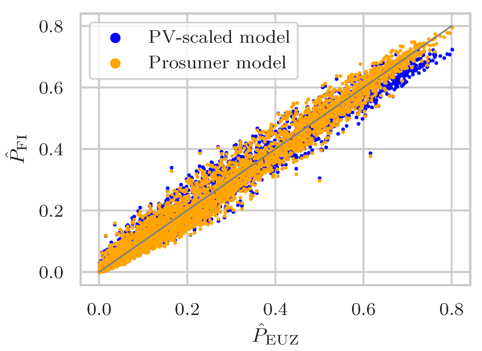
A scatter plot of the modelled PV power feed-in over the EUZ (Figure 3) illustrates an improved concordance of the prosumer model with the EUZ feed-in compared to the “PV-scaled” reference model. The latter exhibits a notable underestimation for high values of PV power feed-in, which will be further discussed in Section 4. In contrast, the prosumer model shows a better agreement with the EUZ over the full range of the specific feed-in values.

For a quantitative assessment, the root mean square error (RMSE) of the absolute feed-in to the EUZ is calculated as follows:

$$\mathrm{RMSE}=\sqrt{\frac{1}{T}{\sum }_t{\left[P_{\mathrm{FI}}\left(t\right)-P_{\mathrm{EUZ}}\left(t\right)\right]}^2},$$

(6)

where the time t runs over all day-time values with positive simulated PV power. These are the times for which at least one modelled PV system is generating, i.e., the sun is above the horizon. The number of these events is denoted by T. A relative RMSE (normalized by the total nominal PV power $P_{\mathrm{nom}}$) of 1.98% for the “PV-scaled” reference model and 1.89% for the prosumer model is found (see

Table 5. RMSE between the aggregated modelled feed-in and the transfer time series EUZ for the reference “PV-scaled” and the simulated prosumer model (absolute and relative to the total nominal power) and relative improvement (Equation (7)).

	Reference Model	Prosumer Model	Relative Improvement
Absolute	7.31 MW	6.99 MW	4.43%
Relative	1.98%	1.89%	4.43%

). This means that the detailed self-consumption modelling yields an improvement of the RMSE as follows:

$$\frac{{\mathrm{RMSE}}_{\mathrm{ref}}-{\mathrm{RMSE}}_{\mathrm{pro}}}{{\mathrm{RMSE}}_{\mathrm{ref}}}=4.43\%,$$

(7)

where ${\mathrm{RMSE}}_{\mathrm{ref}}$/${\mathrm{RMSE}}_{\mathrm{pro}}$ denotes the RMSE of the reference/prosumer model to the EUZ.

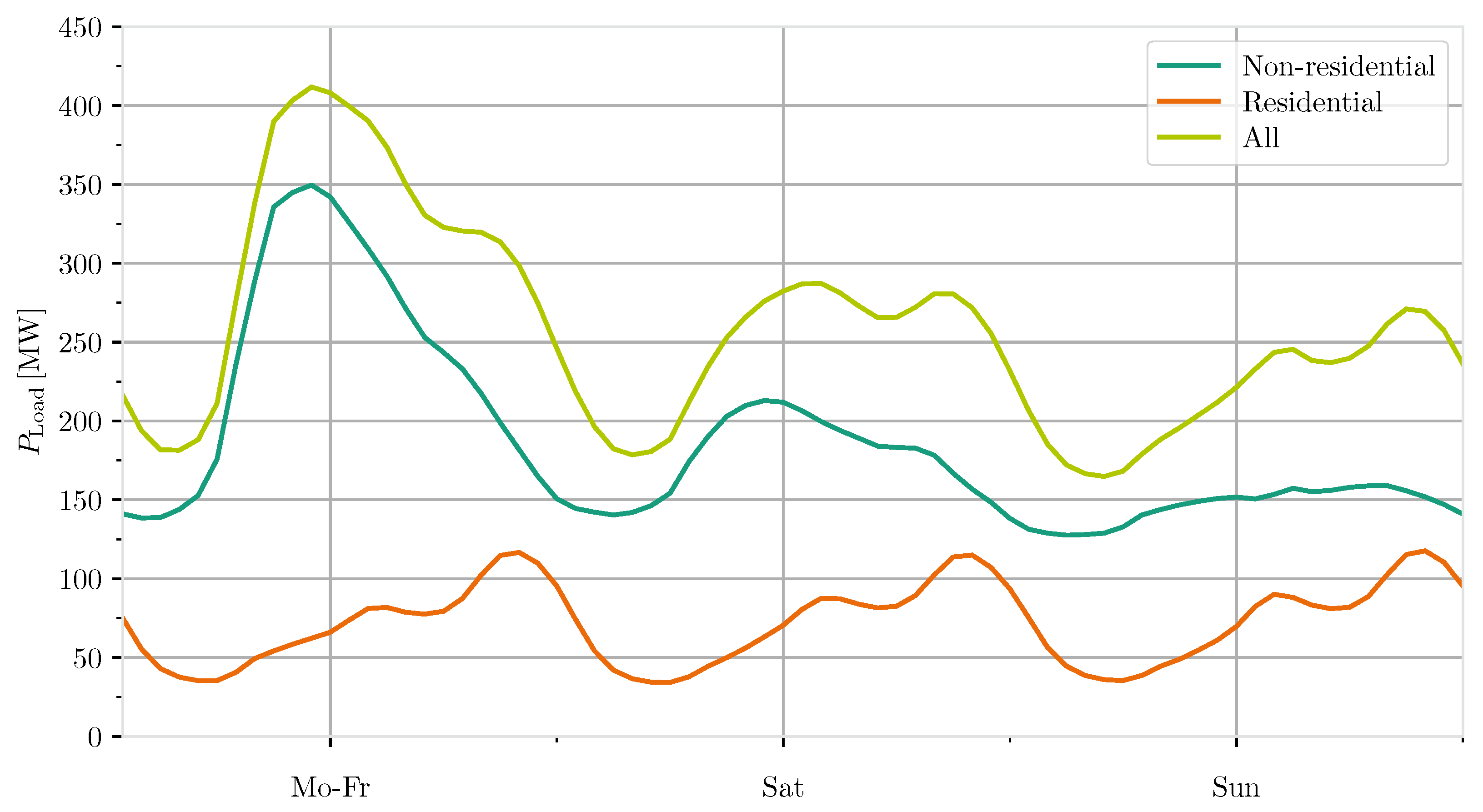
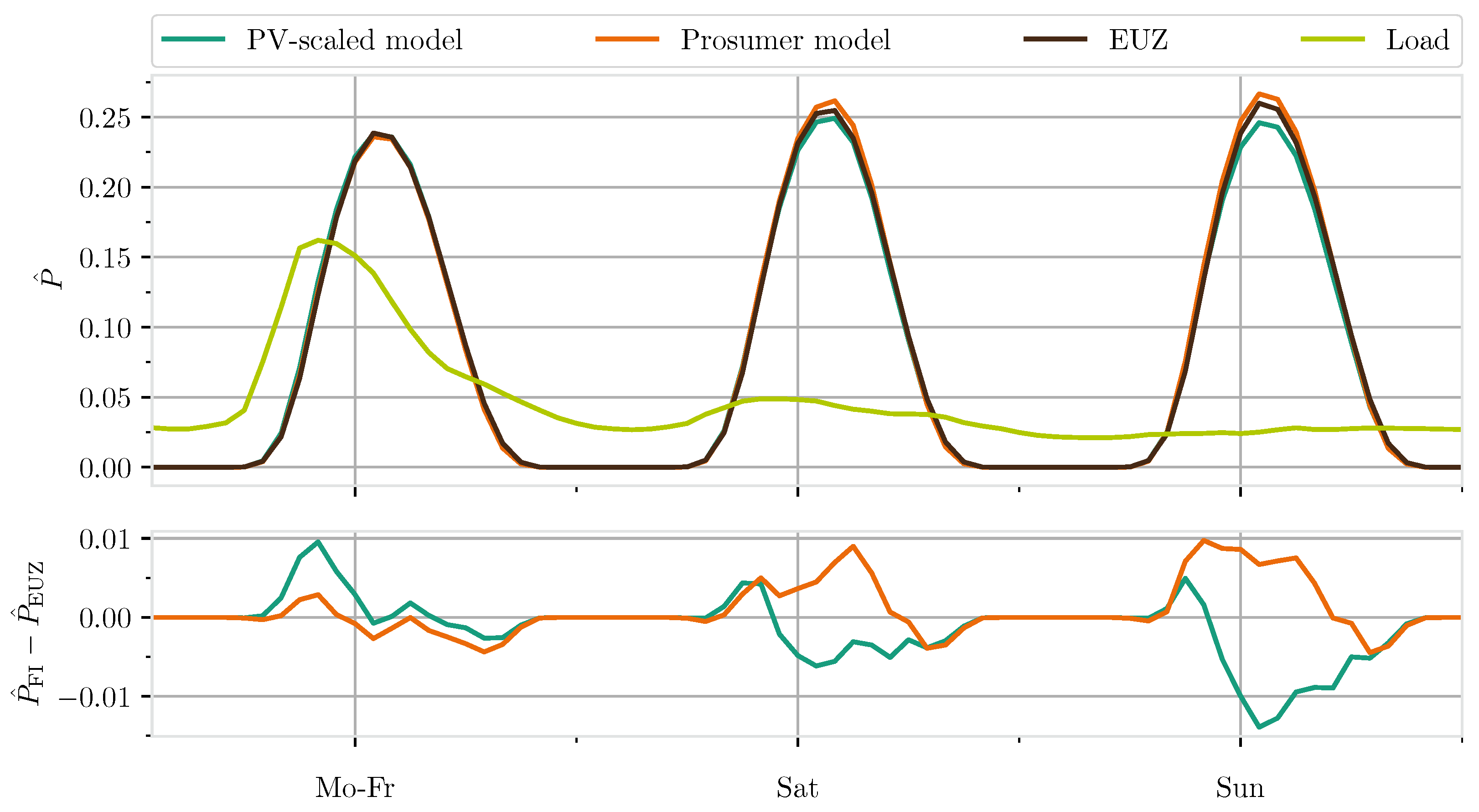
Figure 4 depicts the modelled PV power feed-in to the EUZ in a so-called “type week”. The average daily profiles of the feed-in and load are displayed separately for working days (Monday to Friday), Saturdays and Sundays. The difference in feed-in between the model and the EUZ is shown in the bottom panel. As PV generation evidently does not depend on the day of the week, the profiles for the different type days are very similar in the “PV-scaled” model. In contrast, consumption varies over the course of the week. This is particularly visible here due to the large share of nonresidential prosumers in the SOL validation portfolio (see Table 4). The significantly lower consumption on weekends results in a higher PV power feed-in which is captured by the prosumer model. Compared to the transfer time series EUZ a slight overestimation on weekends is observed in the prosumer model. This effect is, however, smaller in magnitude than the underestimation observed in the “PV-scaled” model. On workdays, the prosumer model shows significantly smaller deviations from the transfer time series EUZ than does the “PV-scaled” model by taking into account higher consumption during morning hours.

In summary, the evaluations confirmed that the prosumer model is capable of representing temporal patterns of measured PV power feed-in. In the studied situation with a small self-consumption rate of less than 10% on average, the improvement by inclusion of realistic consumption in the model is not very large but clearly visible.

4. Model Results and Discussion

The analysis of self-consumption was carried out on the full prosumer model system (see Table 2). As before, all PV systems registered as “designed for self-consumption” were chosen as prosumers, for all other systems full feed-in was assumed. The full model portfolio was studied in comparison with the SOL subportfolio comprising all PV systems with time-resolved measurements. This provides some insight into how far the measurement-based knowledge about the SOL systems can be transferred to the full grid and which further effects emerge. We analysed the self-consumption profiles according to the various parameters affecting PV generation and consumption.

4.1. Variations of Self-Consumption over the Year

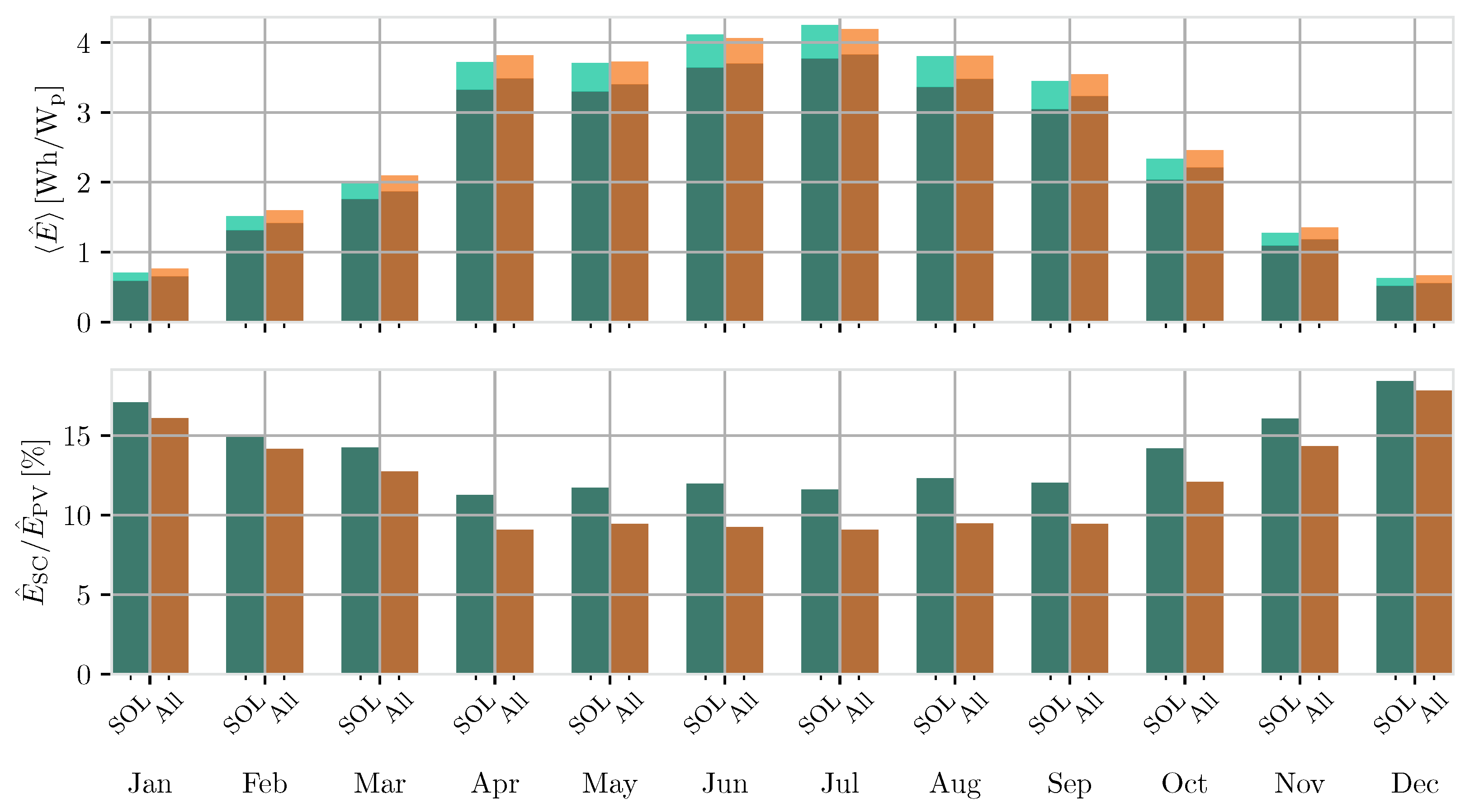
Electricity demand as well as PV generation change during the course of the year, affecting total and relative self-consumption. This seasonal effect is displayed in Figure 5 for the SOL subportfolio and for the full portfolio. The top panel shows monthly values of PV generation split into feed-in and self-consumption; in the bottom panel, the corresponding self-consumption rates are displayed. In each month, the SOL subportfolio exhibits higher self-consumption than does the full portfolio. Averaged of the whole year, self-consumption rates amount to 12% for the SOL subportfolio compared to 9.5% for the full portfolio. This can be attributed to the larger share of nonresidential buildings in the SOL subportfolio where the higher electricity demand (see Figure 2) allows for potentially higher self-consumption.

Higher self-consumption rates during the winter compared to the summer months are observed in both portfolios, reaching more than 17% in the month of December with the least sunlight and, hence, lowest PV generation. In the full portfolio, this is almost twice as high as in the summer months with high PV generation. The seasonal variation is less distinct in the SOL subportfolio where self-consumption rates during summer still reach 10–12%.

4.2. Variation of Self-Consumption with Different Parameters

For insight into the most relevant factors influencing the self-consumption in a portfolio, we examined how its time course correlates with other quantities. This could help identify suitable quantities for a parameterized model of self-consumption based on measurement data.

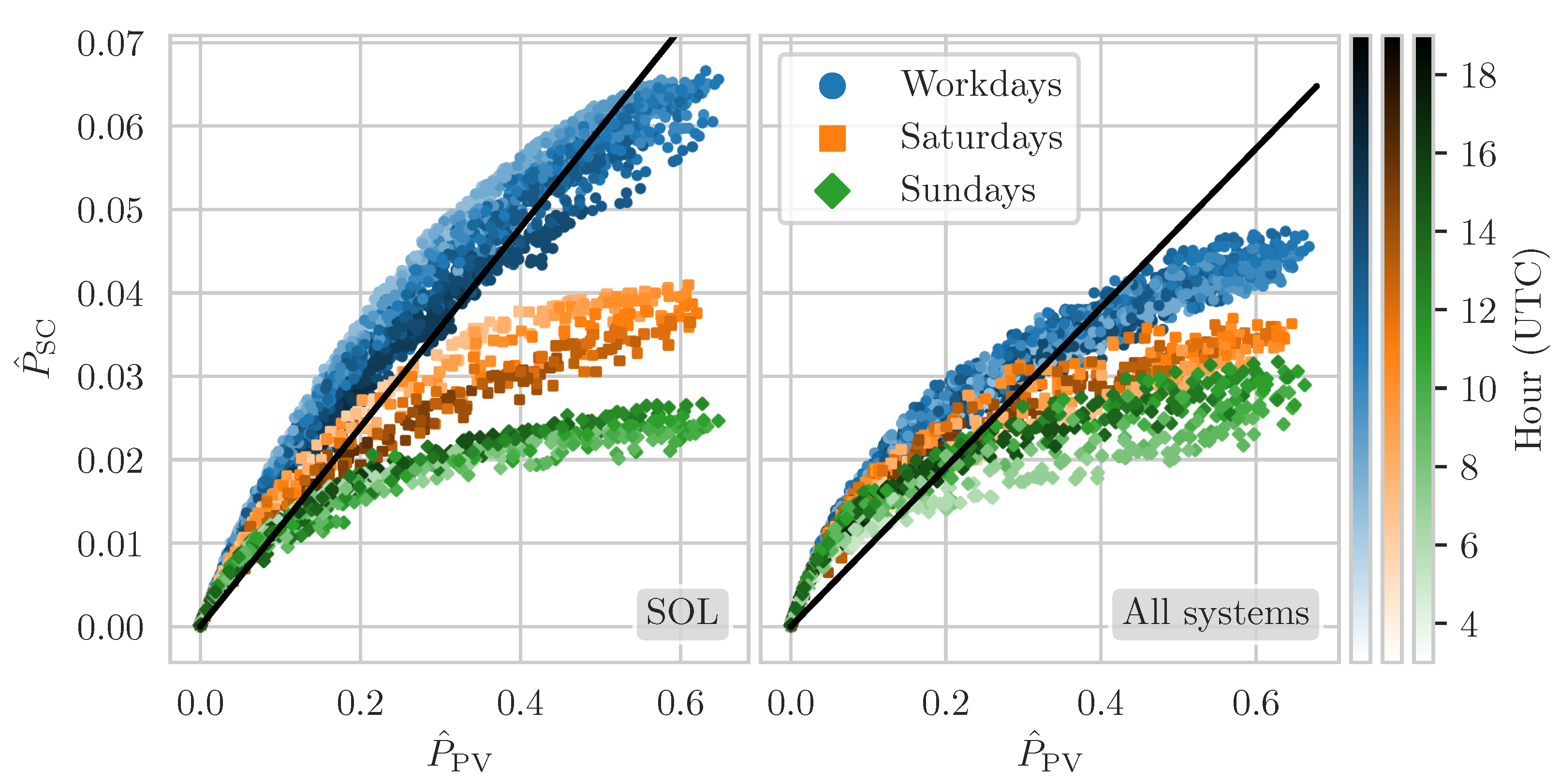
In Figure 6, it can be seen how the total self-consumption relates to the corresponding PV generation at each time step. With higher PV generation, higher values of self-consumption are observed. For the SOL subportfolio, this increase splits into three distinct branches of higher, medium and lower self-consumption for workdays, Saturdays and Sundays, respectively. Additionally, the amount of self-consumption varies with the time of the day inside each branch. At a given level of PV generation, self-consumption is higher in the morning on workdays and Saturdays, whereas on Sundays, self-consumption is higher in the afternoon. In the full model portfolio, the same branching is observed but the differentiation between the days of the week is less pronounced. The trend towards higher self-consumption in the afternoon on weekends appears even stronger, while on workdays, the time of the day appears to have little influence. These effects can be expected from the different load profiles (Figure 2), keeping in mind that the SOL subportfolio is dominated by the nonresidentials whereas the situation is more balanced in the full model portfolio.

The increase of the total self-consumption with PV generation in both portfolios exhibits a clearly nonlinear behaviour with a decreasing slope towards higher values of PV generation. An intuitive explanation of this is that for an increasing number of prosumers, the local PV generation exceeds the local demand, prohibiting a further increase of self-consumption at this site. As a result, the “PV-scaled” reference model indicated by the linear relation (black line) in Figure 6 will generally underestimate self-consumption in situations of low PV generation and overestimate in situations of high PV generation. This was also observable in the validation of both models against measured feed-in (see Figure 3).

From these observations, we draw three central conclusions. First, the assumption that the two portfolios behave differently is strengthened. A feed-in estimate based on the SOL subportfolio only will not adequately reproduce the effects of self-consumption in the full model portfolio. Second, self-consumption varies significantly with the courses of day and week, particularly in the SOL subportfolio. Hence, the day of the week and the time of the day might be relevant quantities for a parametrization of a refined model for PV self-consumption. Third, in a portfolio of PV/prosumer systems, the total self-consumption does not scale linearly with the total PV generation. An appropriate model capturing this nonlinear relation is very likely to generate more satisfactory estimates of self-consumption and feed-in.

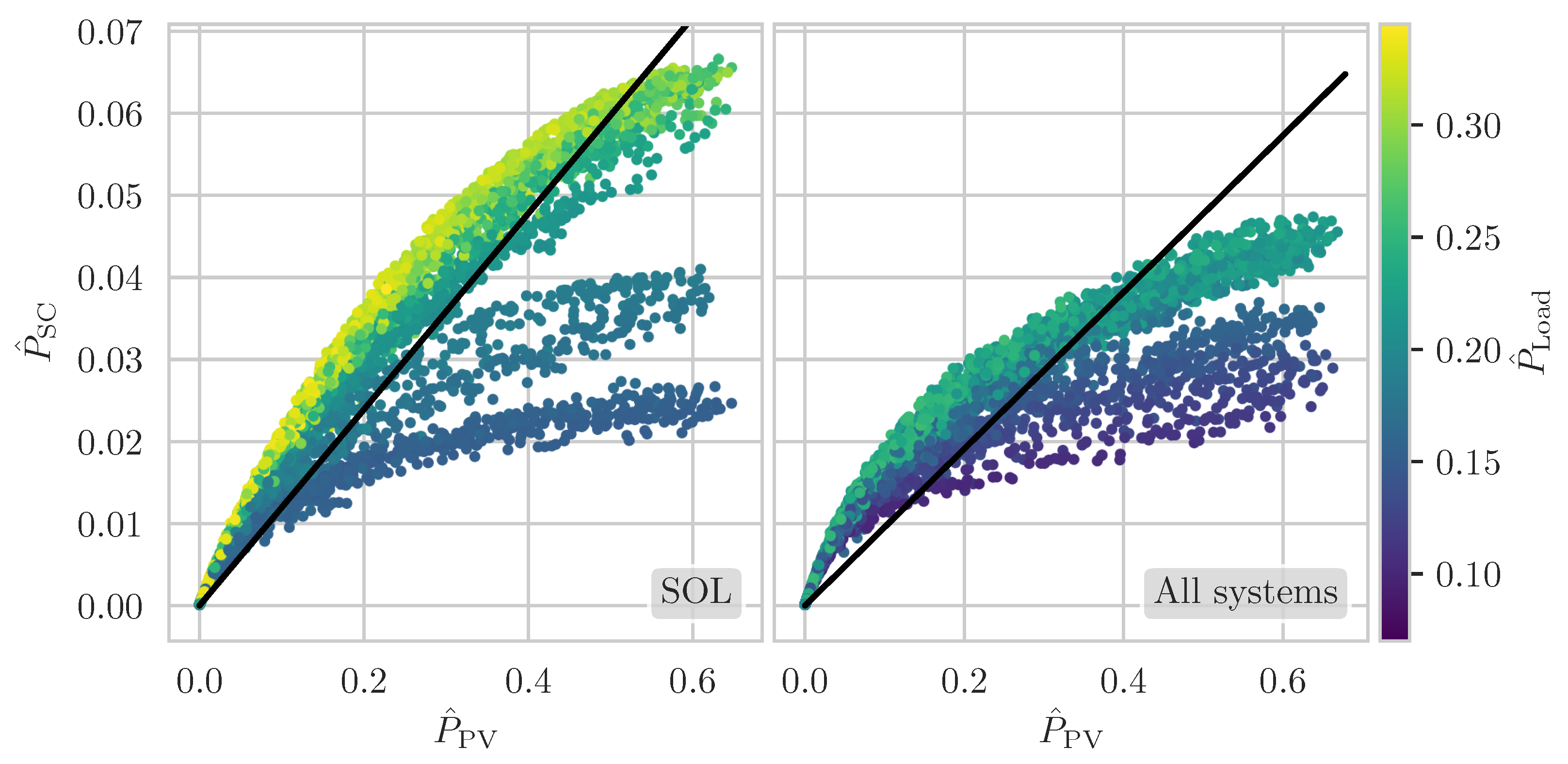
Another natural candidate for the parametrization of a self-consumption model is the total electricity demand of all buildings with PV systems in the grid. In Figure 7, the same data as in Figure 6 are shown with different colouring. Instead of day and time, the colour spectrum represents the corresponding specific load ${\widehat{P}}_{\mathrm{Load}}$. An overall positive correlation between self-consumption and load is observed for any given value of PV generation. The separation into workdays and weekends appears implicit in this parameter, as the latter exhibit lower load values. Similarly, the observed daily cycles in self-consumption seem to be strongly related to different load levels.

From the definition of self-consumption on an individual system level (Equation (1)), an increase of the total self-consumption with the total PV generation and load, as observed above, can be expected. The overall behaviour on a grid level is, however, not as trivial as the distribution of the total energy generation among the individual PV systems, and the distribution of the total load among the individual consumers and the share of prosumers in the grid induce strong nonlinearities. As consequence, parameters relating the total self-consumption to the total PV generation or the total demand necessarily have to be calibrated to the specific PV/prosumer system portfolio.

Post-FIT Scenario

It can be expected that with increasing electricity consumption costs and decreasing FITs, self-consumption will become increasingly attractive. In an extreme case, all PV systems associated with a consumer might act as prosumers. If the prosumer systems in the model portfolio form a representative subset of the full PV system portfolio, it can be expected that the overall self-consumption rate increases with the ratio of installed nominal powers (of all PV systems to the systems designed for self-consumption today, see Table 2) from 9.5% to 29.5%. In a “post-FIT” scenario, we apply the 100% prosumer situation to the model system and examine the effects on the net self-consumption rates. As we keep the PV portfolio constant and do not consider additional technologies like battery storage here, this is not expected to resemble the future reality but rather highlight the possible effects in a certain boundary case. For the simulation of the full system, we find a self-consumption rate of 26.2%, which is in good agreement with the estimate. For the SOL subportfolio, the situation is completely different. The scaling by the installed nominal powers yields a self-consumption rate of 38.0%, while in the simulation, we find 20.4%, indicating that the SOL systems currently designed for self-consumption are not a representative subset of all SOL systems.

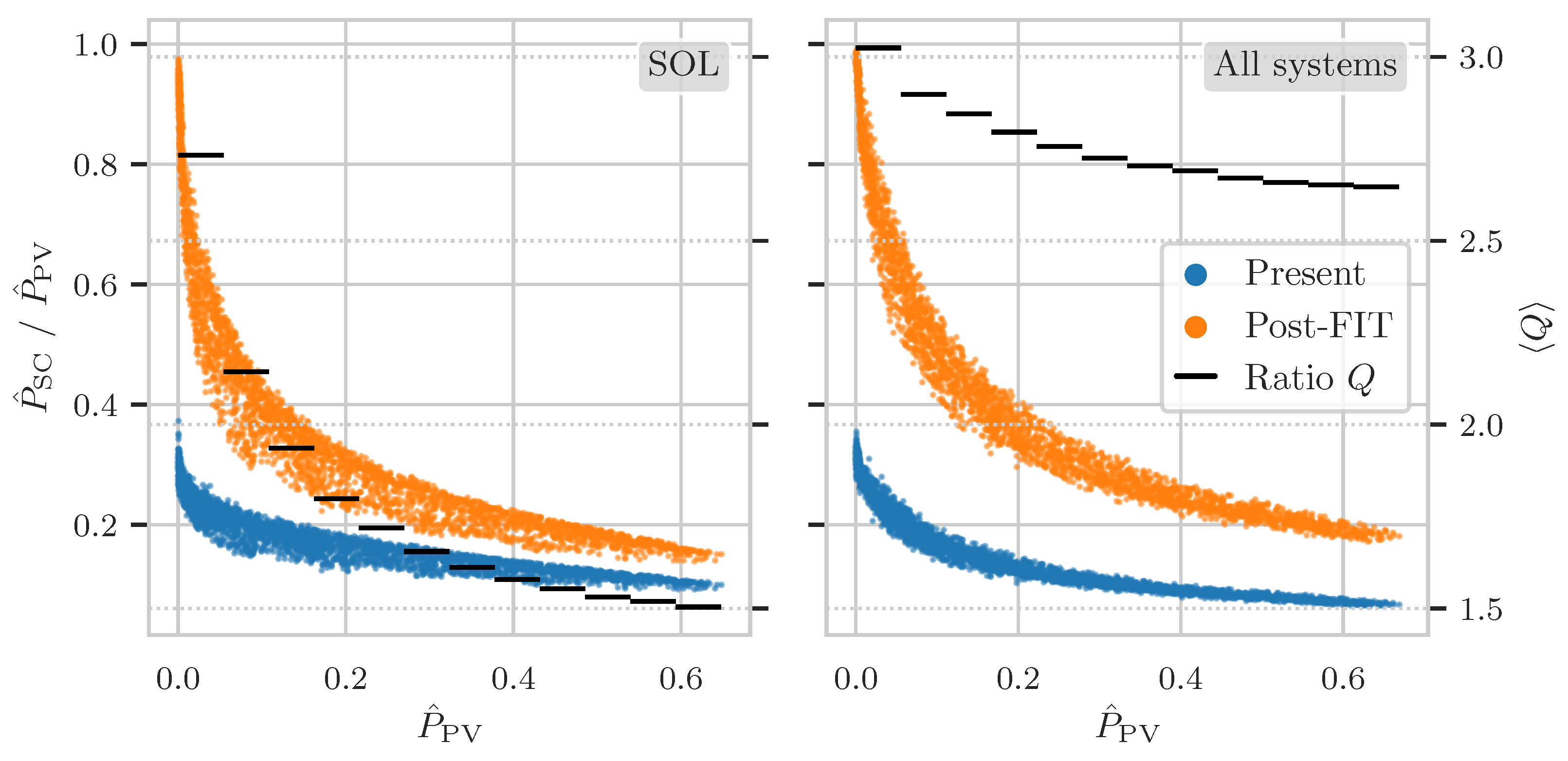
Figure 8 compares the time-dependent self-consumption rate ${\widehat{P}}_{\mathrm{SC}}/{\widehat{P}}_{\mathrm{PV}}$, for the present state and the post-FIT scenario. The observed overall shape of decreasing self-consumption rates with increasing PV generation is similar in either scenario and portfolio. In the “present” scenario, the self-consumption rate decreases from slightly below 40% to a value between 10 and 20% with increasing PV generation in both portfolios, the SOL systems and the full model. In the post-FIT scenario, almost 100% of the produced energy is taken up by self-consumption at low PV generation. With increasing PV generation, the self-consumption rate initially drops faster in the SOL subportfolio than in the full model but reaches a value slightly below 20% at maximum PV generation in both portfolios. In order to quantify the change in self-consumption behaviour, we also show the ratio Q of the self-consumption rate in the present to the post-FIT scenario as bin averages over the full range of PV generation. Compared to the simple estimate based on the nominal PV power mentioned above, Q would be the real scaling factor to predict the future self-consumption from the present state. $\langle Q\rangle$ decreases from 2.75 for low to around 1.5 for high PV generation values in the SOL portfolio. In the full model, the trend is the same, but the variation is much smaller with all values between 2.5 and 3. This confirms the observation that the linear scaling of self-consumption rates (with the ratio of 3.1 of installed nominal powers) is a viable approach in the full model portfolio but not in the SOL subportfolio. Again, we can conclude that the measurement-based knowledge of the behaviour of the SOL subportfolio cannot simply be extrapolated to the full portfolio.

5. Conclusions

In this paper, we introduced a stochastic bottom-up simulation model of PV generation, self-consumption and feed-in for a portfolio of 118,650 PV prosumers. Although statistic deviations at the individual system level are expected, this provides a realistic representation of the situation in a German transmission system and, thus, a valid description at higher levels of aggregation can be assumed. The model builds on established methods for satellite-derived solar irradiance calculations and PV simulations combined with synthetic load profile generation for households and commercial buildings. In the model validation, a deviation of less than 5% to annual meter readings was reached. Furthermore, a relative RMSE of less than 2% (of the nominal power) was obtained in comparison with the aggregated feed-in time series at the distribution grid level. Compared to a linear reference model in which the time dependence is derived from the time course of PV generation only, a relative improvement of more than 4% was observed.

The variation of self-consumption at different time scales was analysed as was the relation to the grid total of PV generation and electric load. These quantities were identified as candidates for the parametrization of a data-driven self-consumption model. Furthermore, several observations strengthen the assumption that the time-dependent behaviour of a grid-level PV/prosumer portfolio cannot simply be deduced from the currently available measurements. In a post-FIT scenario of 100% prosumers as a limiting case, the overall self-consumption rates that can be expected for different PV system portfolios were identified.

Of course, a number of improvements to the model presented here are possible. The use of real PV module orientations and the inclusion of representative industry load profiles or different prosumer strategies could be fruitful and yield quantitatively more precise results. Nevertheless, we are confident that our model system provides reasonable insight into the problem of self-consumption in the present state. Furthermore, it establishes a solid basis for the integration of additional technologies such as battery storage devices, heat pumps or electric cars. In this way, the impact of future technologies and diversifying usage strategies can be studied systematically in different scenarios.

References

1. Karalus, S.; Köpfer, B.; Guthke, P.; Killinger, S.; Lorenz, E. Modelling PV self-consumption at portfolio level. In Proceedings of the 11th Solar & Storage Power System Integration Workshop (SIW 2021), Institution of Engineering and Technology, Berlin, Germany, 28 September 2021; pp. 146–153. [Google Scholar] [CrossRef]
2. Sengupta, M.; Habte, A.; Wilbert, S.; Gueymard, C.; Remund, J. Best Practices Handbook for the Collection and Use of Solar Resource Data for Solar Energy Applications: Third Edition; Technical Report NREL/TP-5D00-77635; National Renewable Energy Lab.: Golden, CO, USA, 2021. [Google Scholar] [CrossRef]
3. Erdener, B.C.; Feng, C.; Doubleday, K.; Florita, A.; Hodge, B.M. A review of behind-the-meter solar forecasting. Renew. Sustain. Energy Rev. 2022, 160, 112224. [Google Scholar] [CrossRef]
4. Lenck, T.; Podewils, C.; Jahn, A. Wie Weiter Nach der EEG-Förderung? Solaranlagen Zwischen Eigenverbrauch und Volleinspeisung; Technical Report 188/01-H-2020/DE; Agora Energiewende: Berlin, Germany, 2020. [Google Scholar]
5. Kächele, R.; Tomschitz, C.; Rongstock, R.; Binder, J. Neue Prosumerlastprofile als Alternative zur Lastgangzählung bei Kleinverbrauchern mit PV-Anlage. In Online-PV-Symposium; Conexio GmbH: Pforzheim, Germany, 2021; pp. 53–62. [Google Scholar]
6. Günnewig, D.; Püschel, M.; Schicketanz, S.; Kinast, P.; Thylmann, M.; Nazerian, V.; Kelm, T.; Metzger, J.; Jachmann, H. Vorbereitung und Begleitung bei der Erstellung eines Erfahrungsberichts gemäß § 97 Erneuerbare-Energien-Gesetz. Teilvorhaben II c: Solare Strahlungsenergie; Bundesministerium für Wirtschaft und Energie: Berlin, Germany, 2019. [Google Scholar]
7. Günther, C.; Schill, W.P.; Zerrahn, A. Prosumage of solar electricity: Tariff design, capacity investments, and power sector effects. Energy Policy 2021, 152, 112168. [Google Scholar] [CrossRef]
8. Enervis. Mittelfristprognose zur Deutschlandweiten Stromerzeugung aus EEG-Geförderten Kraftwerken für die Kalenderjahre 2021 bis 2025. 2020. Available online: https://www.netztransparenz.de/EEG/Mittelfristprognosen/Mittelfristprognose-2021-2025 (accessed on 13 February 2023).
9. Wirth, H. Aktuelle Fakten zur Photovoltaik in Deutschland; Technical Report; Fraunhofer ISE. 2023. Available online: https://www.ise.fraunhofer.de/de/veroeffentlichungen/studien/aktuelle-fakten-zur-photovoltaik-in-deutschland.html (accessed on 1 March 2023).
10. Bahramara, S.; Mazza, A.; Chicco, G.; Shafie-khah, M.; Catalão, J.P. Comprehensive review on the decision-making frameworks referring to the distribution network operation problem in the presence of distributed energy resources and microgrids. Int. J. Electr. Power Energy Syst. 2020, 115, 105466. [Google Scholar] [CrossRef]
11. Balestrieri, M.; James, A.; Kedis, M.; Gonzales, F.M. Mitigation of Grid Susceptibility Caused by Behind-the-Meter Solar Generation. In Proceedings of the 2020 IEEE Conference on Technologies for Sustainability (SusTech), Santa Ana, CA, USA, 23–25 April 2020; pp. 1–8. [Google Scholar] [CrossRef]
12. Ciocia, A.; Amato, A.; Di Leo, P.; Fichera, S.; Malgaroli, G.; Spertino, F.; Tzanova, S. Self-Consumption and Self-Sufficiency in Photovoltaic Systems: Effect of Grid Limitation and Storage Installation. Energies 2021, 14, 1591. [Google Scholar] [CrossRef]
13. Hawker, G.S.; Bell, K.R.W. Making energy system models useful: Good practice in the modelling of multiple vectors. WIREs Energy Environ. 2020, 9, e363. [Google Scholar] [CrossRef]
14. Safarazi, S.; Deissenroth-Uhrig, M.; Bertsch, V. Assessing the Impacts of Community Energy Storage Systems on the German Electricity Market: An Agent-based Analysis. In Proceedings of the 2020 17th International Conference on the European Energy Market (EEM), Stockholm, Sweden, 16–18 September 2020; pp. 1–6. [Google Scholar] [CrossRef]
15. Sarfarazi, S.; Sasanpour, S.; Cao, K.K. Improving energy system design with optimization models by quantifying the economic granularity gap: The case of prosumer self-consumption in Germany. Energy Rep. 2023, 9, 1859–1874. [Google Scholar] [CrossRef]
16. Bu, F.; Dehghanpour, K.; Yuan, Y.; Wang, Z.; Zhang, Y. A Data-Driven Game-Theoretic Approach for Behind-the-Meter PV Generation Disaggregation. IEEE Trans. Power Syst. 2020, 35, 3133–3144. [Google Scholar] [CrossRef] [Green Version]
17. Bundesnetzagentur. Marktstammdatenregister. Available online: https://www.bundesnetzagentur.de/DE/Sachgebiete/ElektrizitaetundGas/Unternehmen_Institutionen/DatenaustauschundMonitoring/Marktstammdatenregister/MaStR_node.html (accessed on 15 May 2020).
18. OpenStreetMap Contributors. Available online: www.openstreetmap.org (accessed on 13 February 2023).
19. Karalus, S.; Reise, C.; Zech, T.; Holland, N.; Herzberg, W.; AlSayegh, G.; Killinger, S.; Lorenz, E.; Guthke, P. PV Eigenverbrauch: Hochaufgelöste Modellierung von PV-Erzeugung und Verbrauch für verbesserte Einspeiseprognosen. In Online-PV-Symposium; Conexio GmbH: Pforzheim, Germany, 2020; pp. 758–772. [Google Scholar]
20. Müller, B.; Hardt, L.; Armbruster, A.; Kiefer, K.; Reise, C. Yield predictions for photovoltaic power plants: Empirical validation, recent advances and remaining uncertainties. Prog. Photovoltaics Res. Appl. 2016, 24, 570–583. [Google Scholar] [CrossRef]
21. Hammer, A.; Heinemann, D.; Hoyer, C.; Kuhlemann, R.; Lorenz, E.; Müller, R.; Beyer, H.G. Solar energy assessment using remote sensing technologies. Remote Sens. Environ. 2003, 86, 423–432. [Google Scholar] [CrossRef]
22. Perez, R.; Ineichen, P.; Maxwell, E.L.; Seals, R.; Zelenka, A. Dynamic Global-to-Direct Irradiance Conversion Models. Ashrae Trans. 1992, 98, 354–369. [Google Scholar]
23. Perez, R.; Ineichen, P.; Seals, R.; Michalsky, J.; Stewart, R. Modeling daylight availability and irradiance components from direct and global irradiance. Sol. Energy 1990, 44, 271–289. [Google Scholar] [CrossRef] [Green Version]
24. Saint-Drenan, Y.M.; Good, G.H.; Braun, M. A probabilistic approach to the estimation of regional photovoltaic power production. Sol. Energy 2017, 147, 257–276. [Google Scholar] [CrossRef] [Green Version]
25. Killinger, S.; Lingfors, D.; Saint-Drenan, Y.M.; Moraitis, P.; van Sark, W.; Taylor, J.; Engerer, N.A.; Bright, J.M. On the search for representative characteristics of PV systems: Data collection and analysis of PV system azimuth, tilt, capacity, yield and shading. Sol. Energy 2018, 173, 1087–1106. [Google Scholar] [CrossRef] [Green Version]
26. Saint-Drenan, Y.M. A Probabilistic Approach to the Estimation of Regional Photovoltaic Power Generation Using Meteorological Data: Application of the Approach to the German Case. Ph.D. Thesis, Universität Kassel, Kassel, Germany, 2016. [Google Scholar]
27. Fischer, D.; Härtl, A.; Wille-Haussmann, B. Model for electric load profiles with high time resolution for German households. Energy Build. 2015, 92, 170–179. [Google Scholar] [CrossRef]
28. Statistische Ämter des Bundes und der Länder. Zensus 2011 Datenbank. 2011. Available online: https://ergebnisse2011.zensus2022.de/datenbank/online (accessed on 11 November 2019).
29. Eurostat. Harmonised European Time Use Surveys: 2008 Guidelines; Methodologies and Working Papers; European Communities: Luxembourg, 2009. [Google Scholar]
30. Wille-Haussmann, B.; Fischer, D.; Ohr, F.; Köpfer, B.; Wittwer, C.; Bercher, S.; Engelmann, P. synGHD—Synthetische Lastprofile für eine Effiziente Versorgungsplanung für nicht-Wohngebäude: Abschlussbericht; Technical Report; Fraunhofer-Institut für Solare Energiesysteme: Freiburg, Germany, 2020. [Google Scholar] [CrossRef]
31. Hersbach, H.; Bell, B.; Berrisford, P.; Biavati, G.; Horányi, A.; Muñoz Sabater, J.; Nicolas, J.; Peubey, C.; Radu, R.; Rozum, I.; et al. ERA5 Hourly Data on Single Levels from 1979 to Present. Copernicus Climate Change Service (C3S) Climate Data Store (CDS). 2018. Available online: https://cds.climate.copernicus.eu/cdsapp#!/dataset/reanalysis-era5-single-levels?tab=overview (accessed on 17 August 2020).
32. Statstisches Landesamt Baden-Württemberg. Unternehemensregister. Available online: https://www.statistik-bw.de/ (accessed on 16 June 2020).
33. Statistisches Landesamt Baden-Württemberg. Energiebilanz Baden-Württemberg 2016. Available online: http://www.lak-energiebilanzen.de/energiebilanzen/ (accessed on 16 June 2020).
34. Kleeberger, H.; Hardi, L.; Geiegr, B. Erstellen der Anwendungsbilanzen 2013 bis 2016 für den Sektor Gewerbe, Handel und Dienstleistungen (GHD); Technical Report; Lehrstuhl für Energiewirtschaft und Anwendungtechnik, Technische Universität München: Munich, Germany, 2018. [Google Scholar]
35. Neser, S.; Neiber, J.; Bonkoss, K. Stromverbrauch und Energieeffizienz in der Tierhaltung. In Proceedings of the Energiewende und Landwirtschaft—Landtechnische Jahrestagung, Bad Staffelstein, Germany, 22 November 2012. [Google Scholar]
Figure 1. Distributions of azimuth (left) and tilt angles (right) of the PV systems to be simulated (in blue) and reference systems (in orange) by nominal power classes. In the legend, both the numbers N of the sampled PV systems to be simulated and the reference systems for each class are given. The tilt angles for smaller systems often take high values (steeper roof inclinations of smaller residential buildings), low values for medium-sized systems (flatter roof inclination of large commercial buildings and rack mounting on flat roofs) and intermediate values for large systems (optimised for maximum energy yield). The azimuth angles are increasingly concentrated to the south as the nominal power increases (transition from available roof orientations to yield-optimised south orientations).
Energies 16 03059 g001
Figure 2. Mean electric load on workdays, Saturdays and Sundays for residential buildings, nonresidential buildings and the whole consumption model.
Energies 16 03059 g002
Figure 3. Scatter plot of the aggregated specific feed-in as modelled time series vs. measured transfer time series EUZ for the “PV-scaled” reference model and the prosumer model.
Energies 16 03059 g003
Figure 4. (Top) Type week of specific feed-in in the “PV-scaled” reference model and the prosumer model in comparison with the transfer time series EUZ and the specific load. (Bottom) Specific feed-in difference between the two models and the EUZ in the type weeks above.
Energies 16 03059 g004
Figure 5. Course of self-consumption over the year. (Top) Monthly average of daily specific PV generation split into feed-in (dark colours) and self-consumption (light colours) for the SOL (green)/complete model (orange) portfolios. (Bottom) Corresponding self-consumption rates per month.
Energies 16 03059 g005
Figure 6. Dependency of self-consumption on PV generation and time of day for the SOL (left) and the complete model (right) portfolios. The scatter symbols show the specific self-consumption P ^ SC and PV generation P ^ PV for each time step separated into workdays (blue circles), Saturdays (orange squares) and Sundays (green diamonds). The colours are shaded by the time of the day from morning (light) to evening (dark). The black lines indicate the relation between self-consumption and PV generation as predicted by the linear “PV-scaled” reference model based on the modelled overall self-consumption rates.
Energies 16 03059 g006
Figure 7. Dependency of self-consumption on PV generation and load for the SOL (left) and the complete model (right) portfolios. The scatter symbols show the specific self-consumption P ^ SC and PV generation P ^ PV for each time step coloured by the corresponding specific load P ^ Load . The black lines indicate the relation between self-consumption and PV generation as predicted by the linear “PV-scaled” reference model based on the modelled overall self-consumption rates.
Energies 16 03059 g007
Figure 8. Dependency of the self-consumption rate on PV generation in a post-FIT scenario of 100% prosumer systems compared with the present share for the SOL (left panel) and the complete model (right panel) portfolios. The scatter dots show the instantaneous share of self-consumption on PV generation P ^ SC / P ^ PV (left scale) for the present (blue) and post-FIT scenario (orange). The black lines depict the average ratio Q between future and present self-consumption shares in the indicated intervals (right scale). For a better visualisation, only data for working days are shown here.
Energies 16 03059 g008