
Quantitative Evaluation of the Effects of Heat Island on Building Energy Simulation: A Case Study in Wuhan, China

Abstract
:1. Introduction
2. Methodology
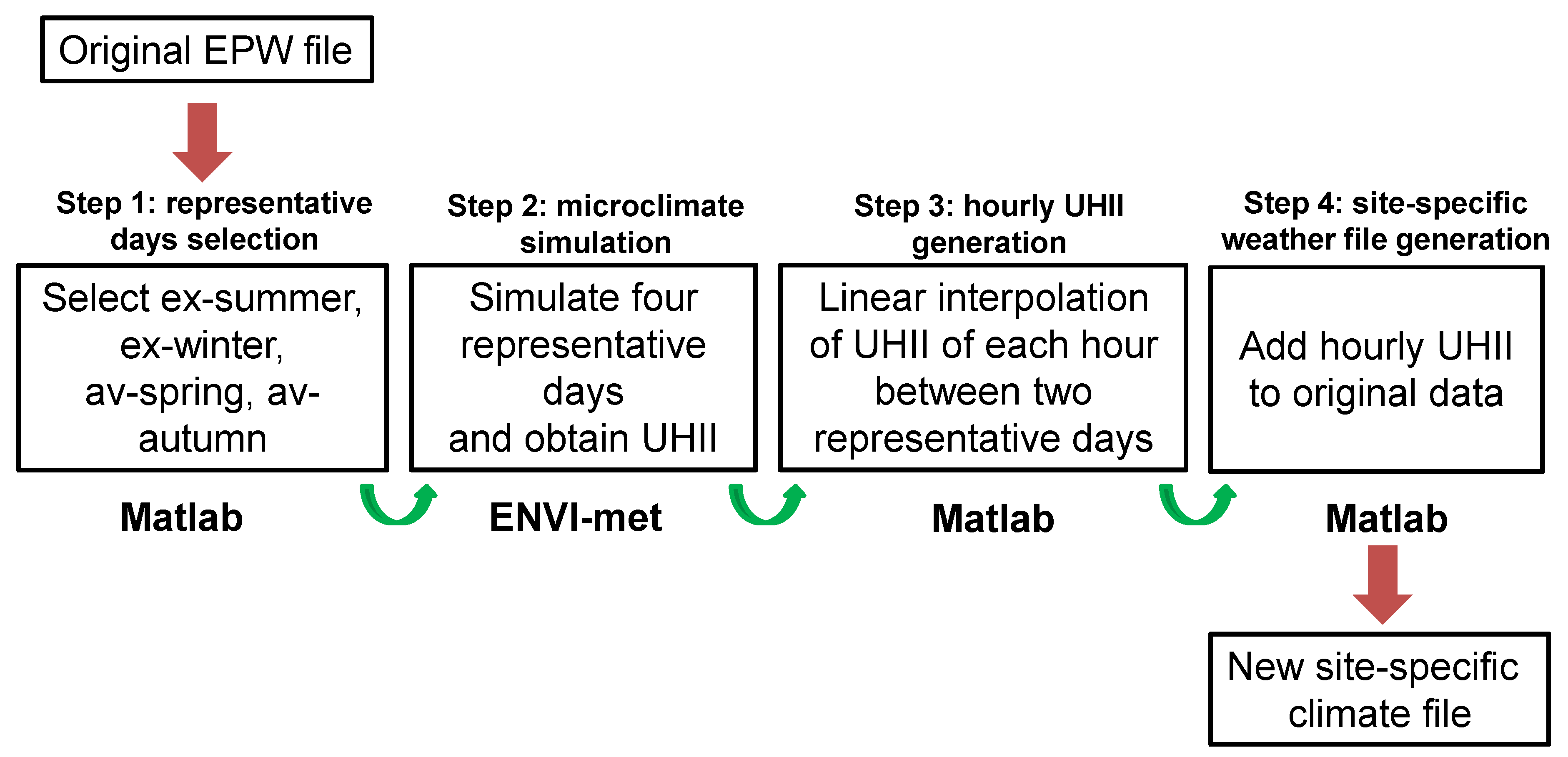
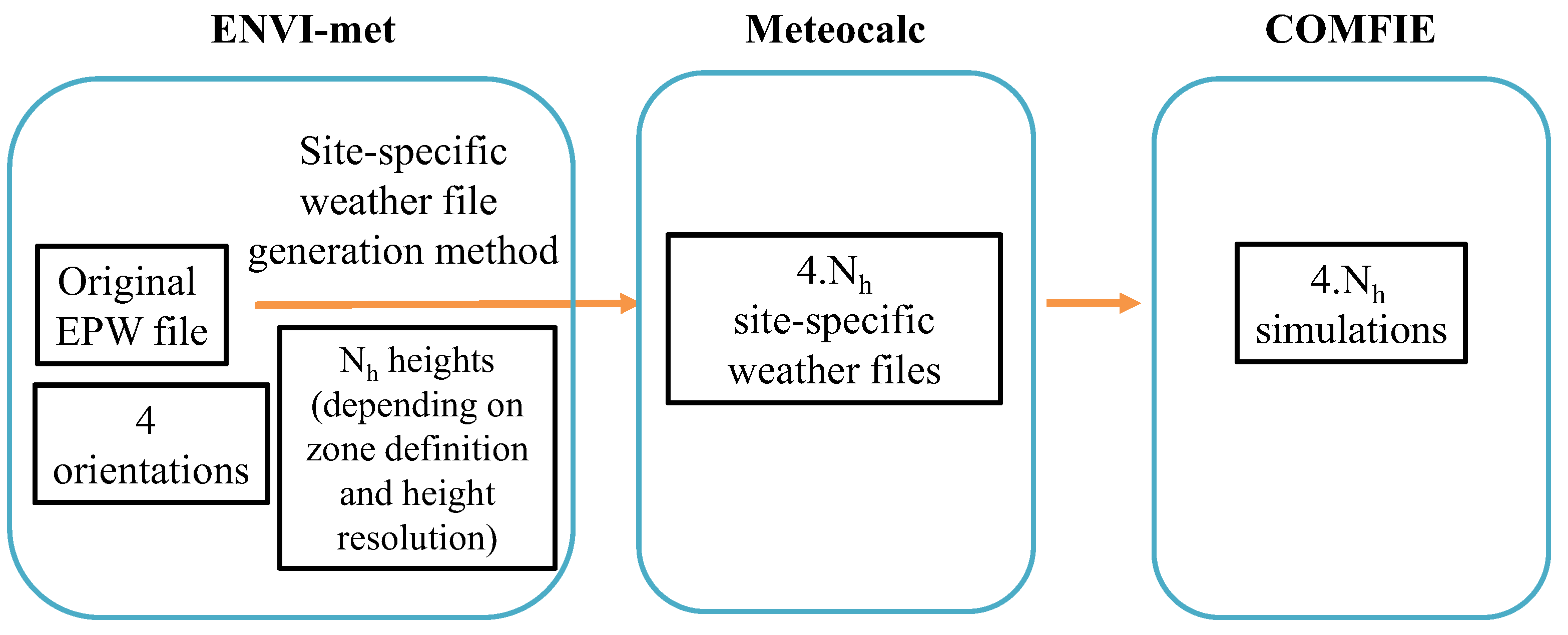
2.1. Site-Specific Weather File Generation Method
2.2. Coupling Microclimate Simulation Tool with DBES Tool
3. Case Study
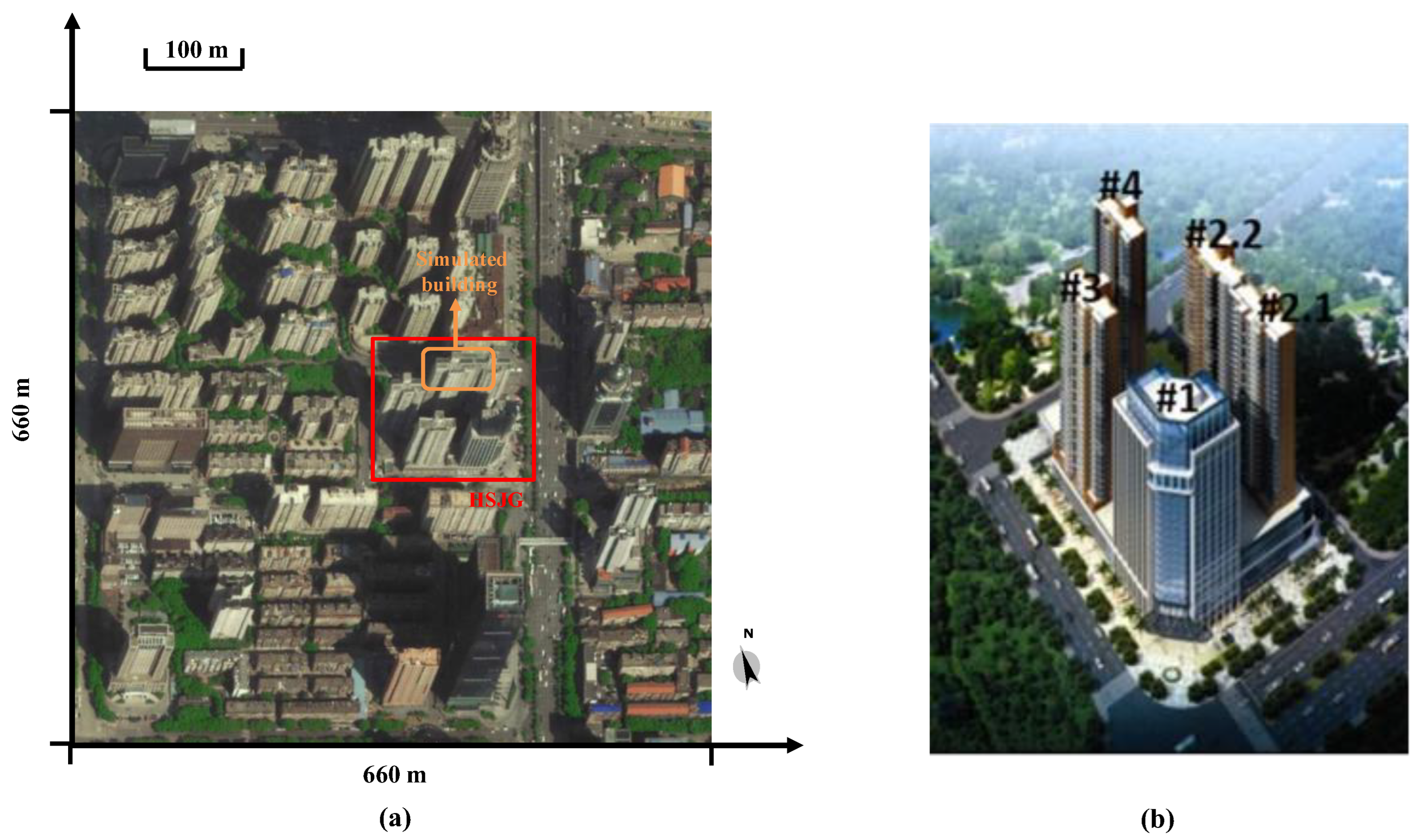
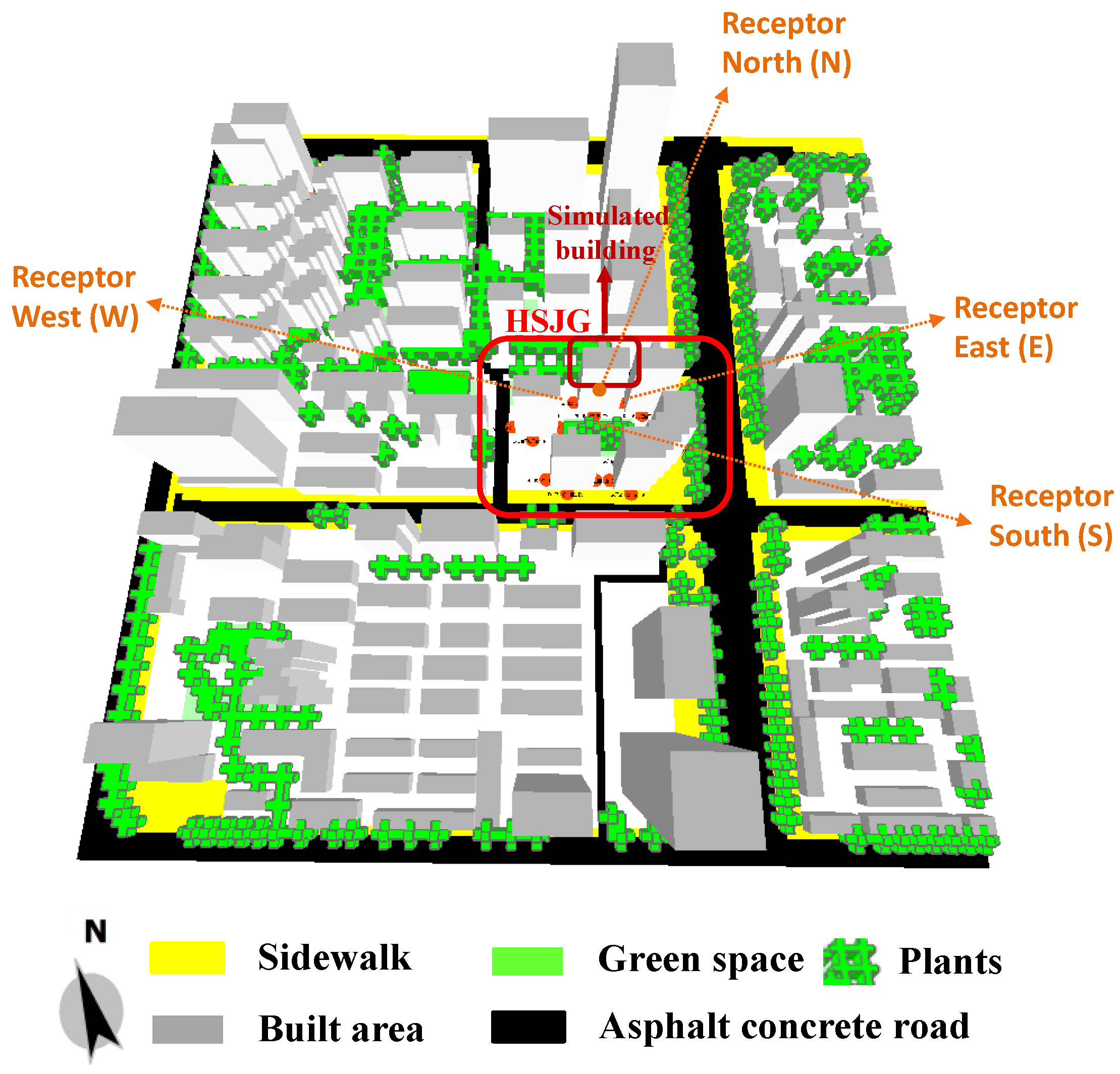
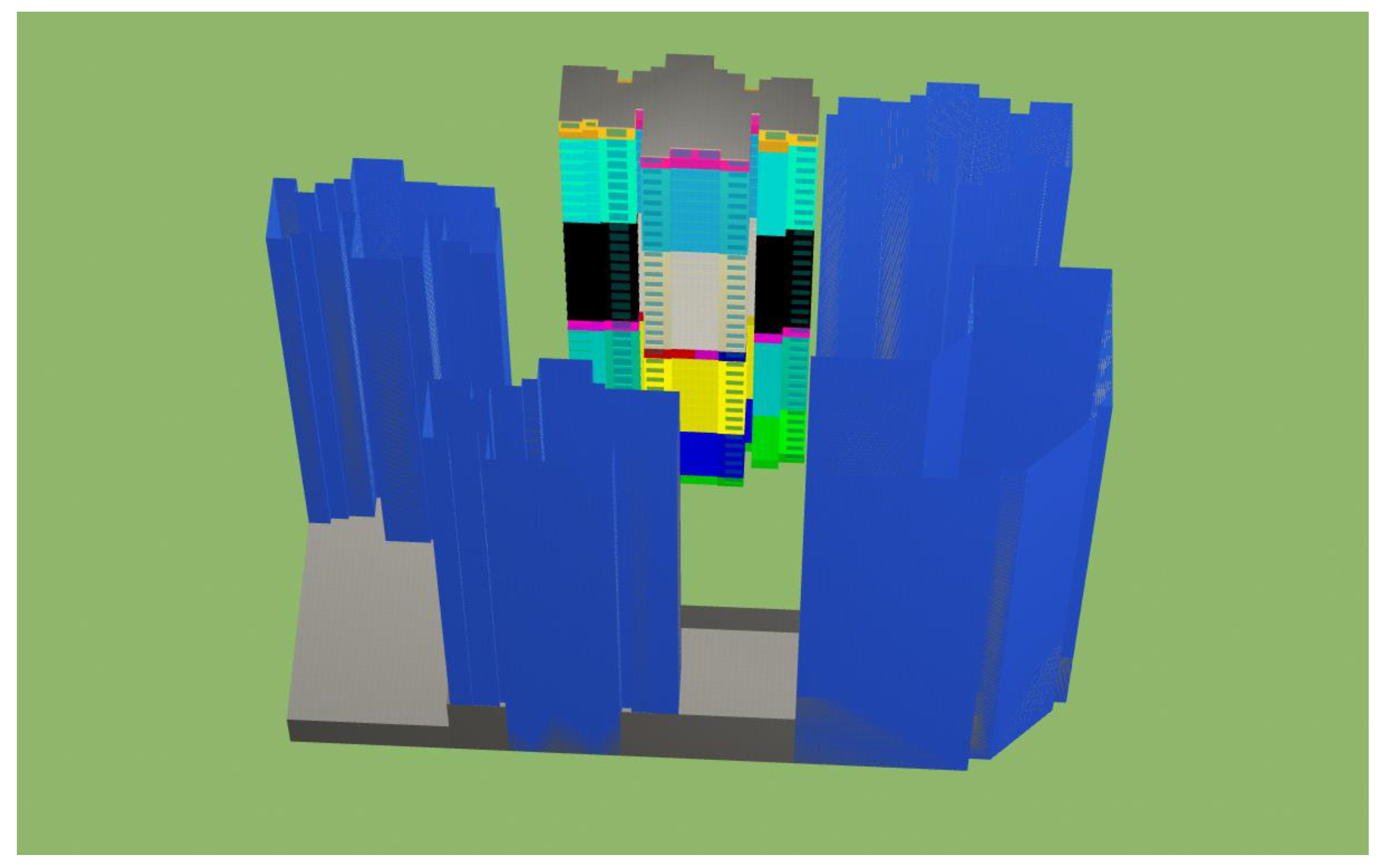
3.1. Basic Information
3.2. Microclimate Simulation Configuration
3.2.1. Representative Days Selection
3.2.2. Simulation Configuration
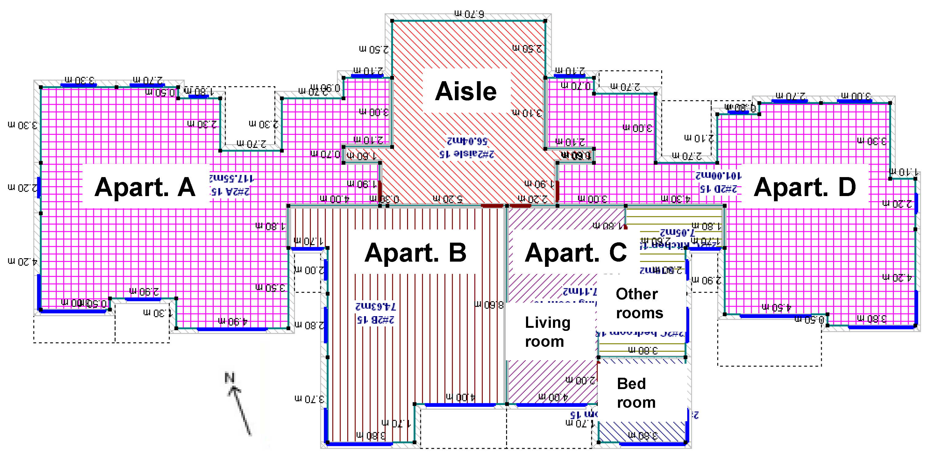
3.3. DBES Configuration
4. Results and Discussion
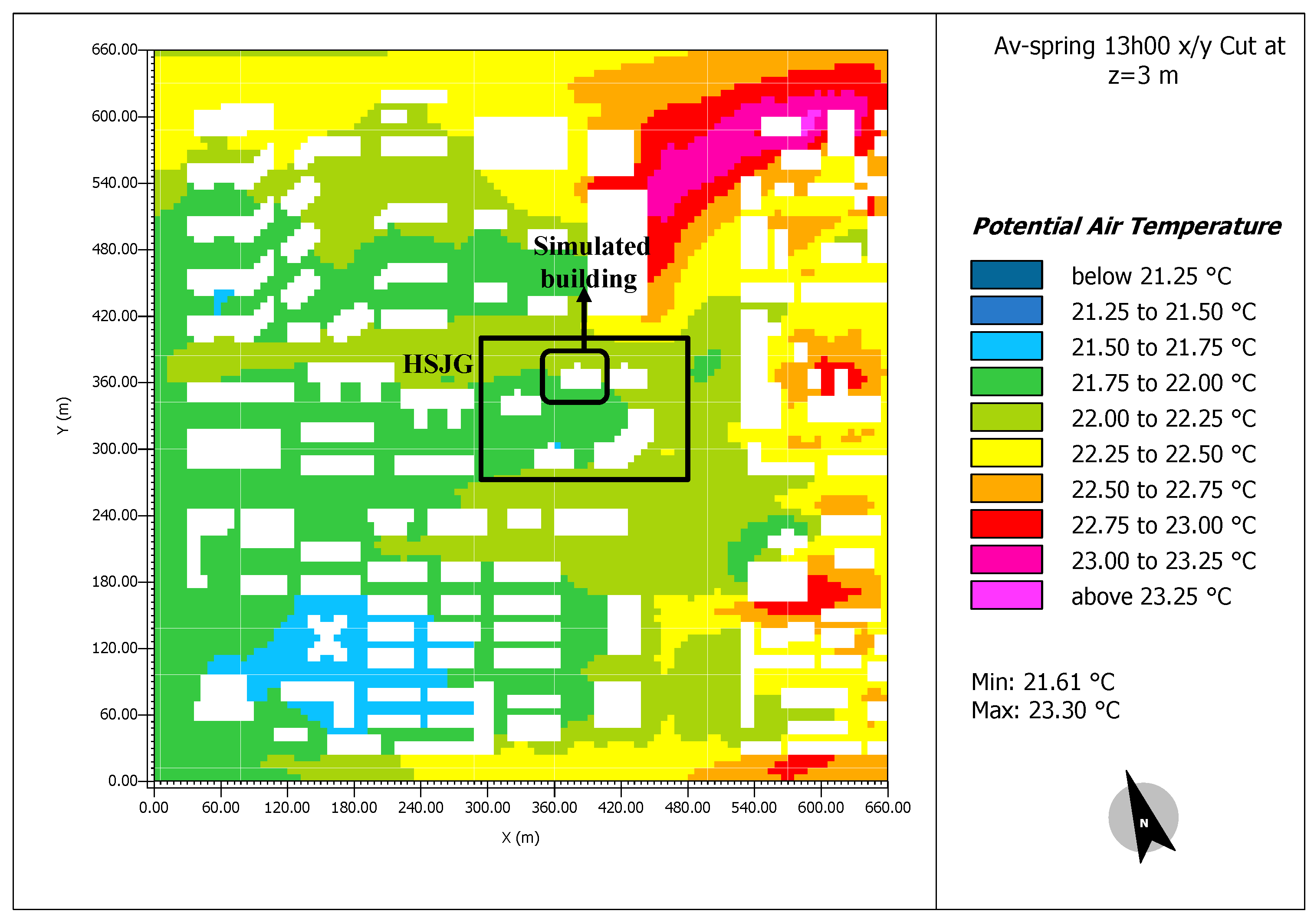
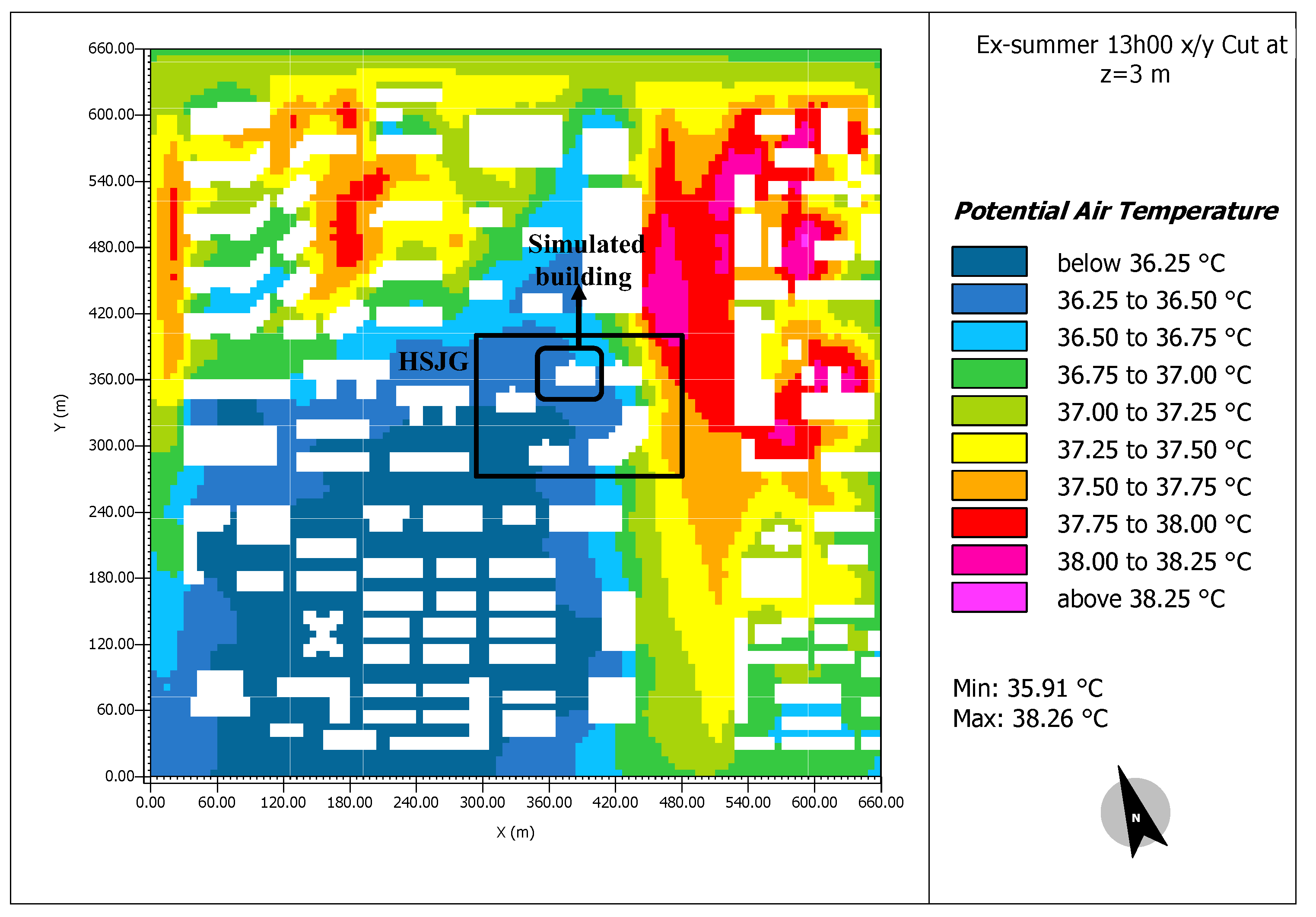
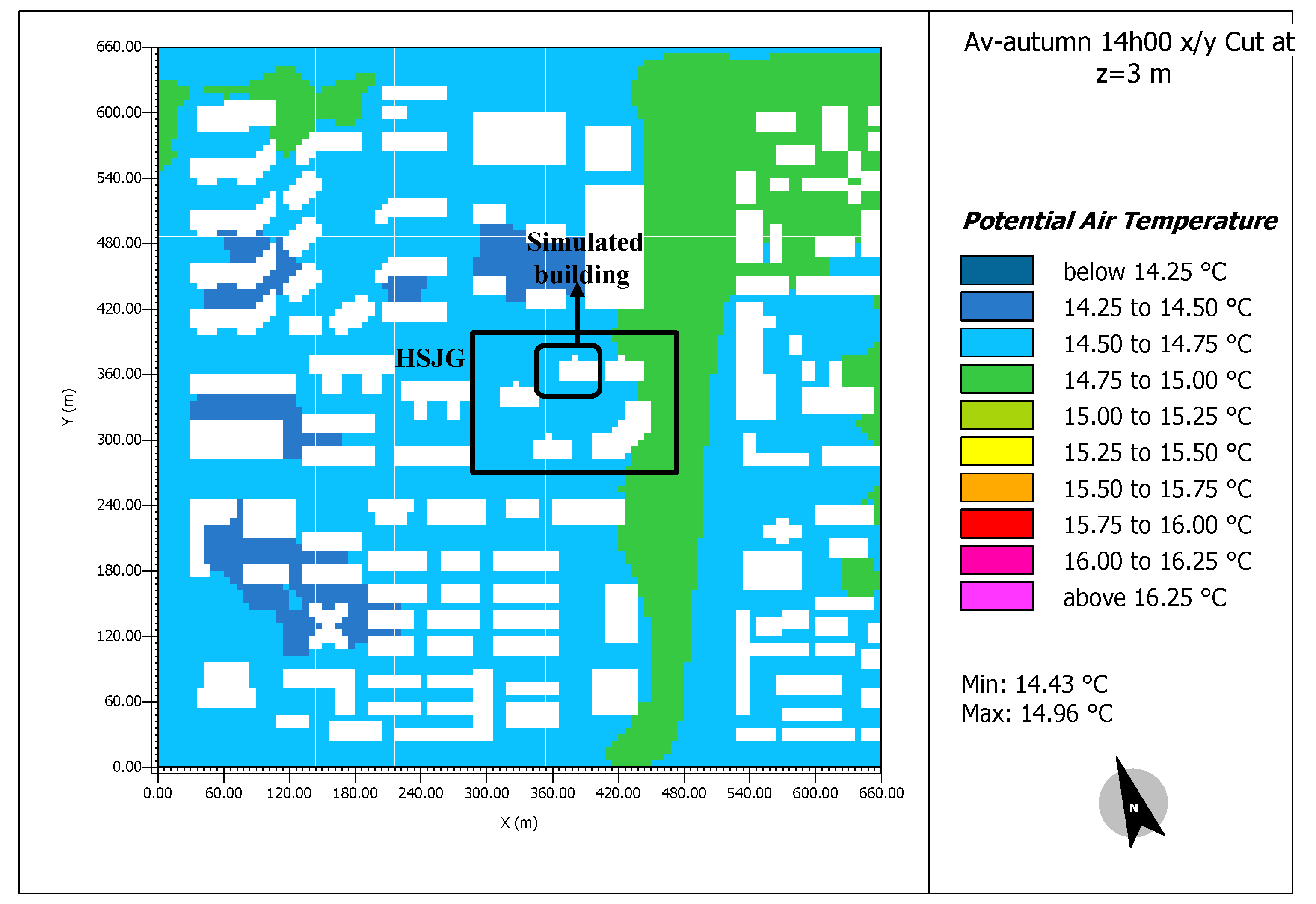
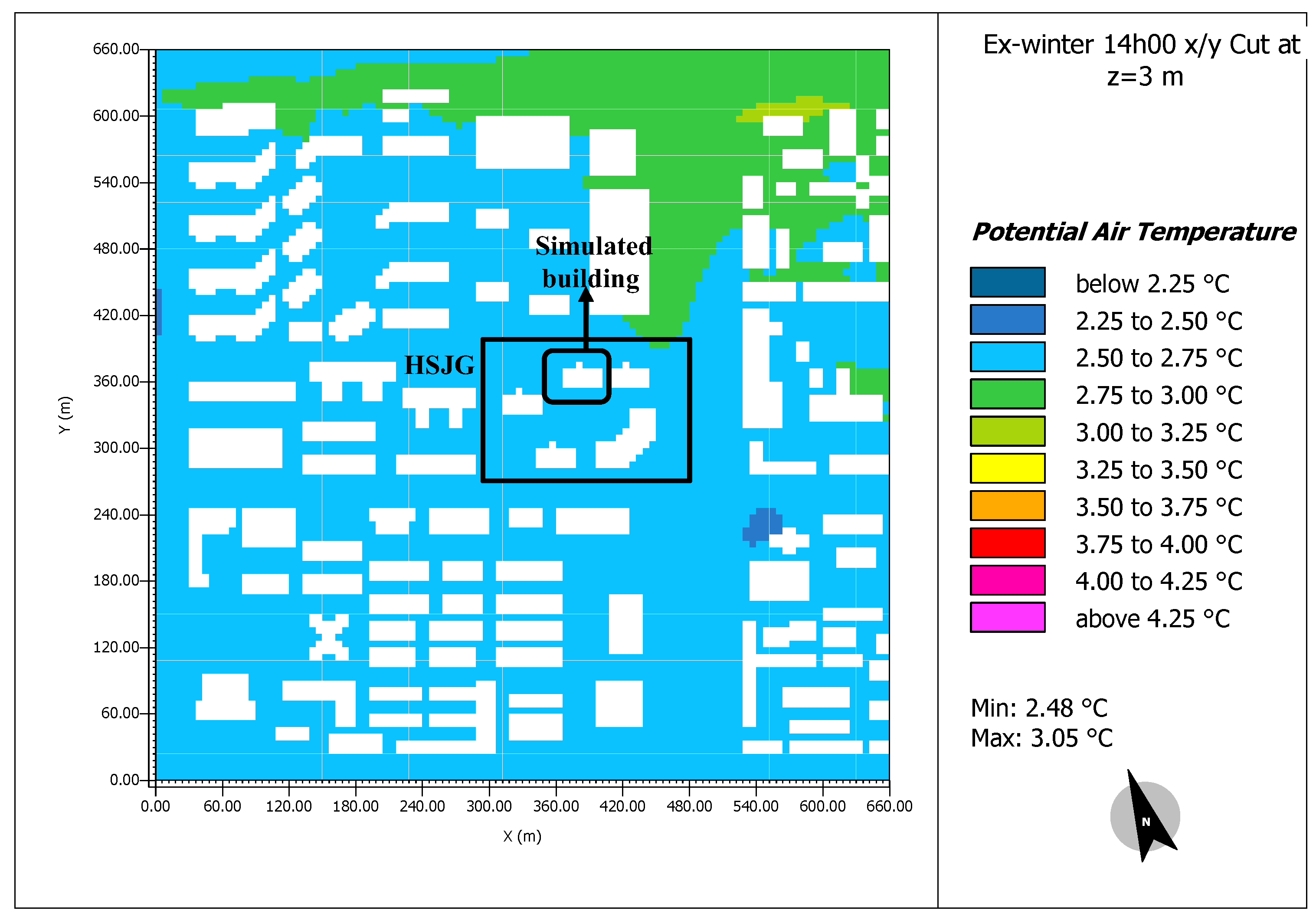
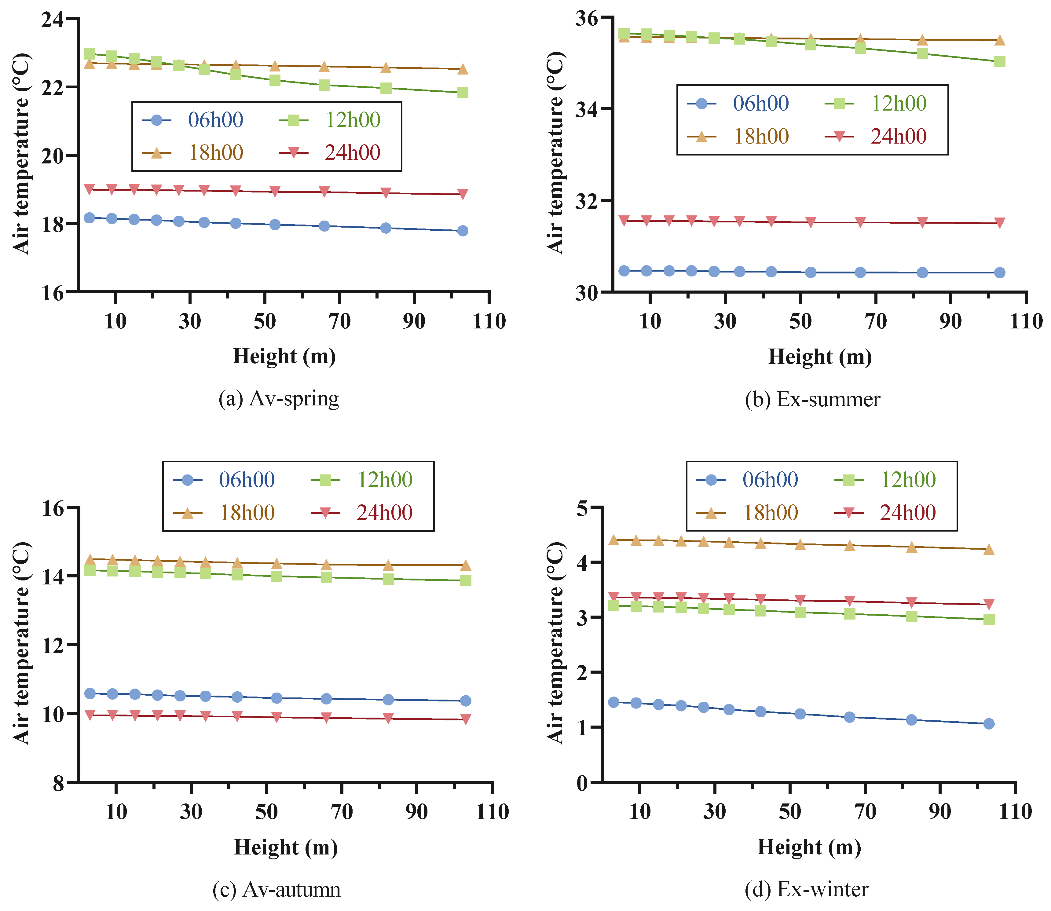
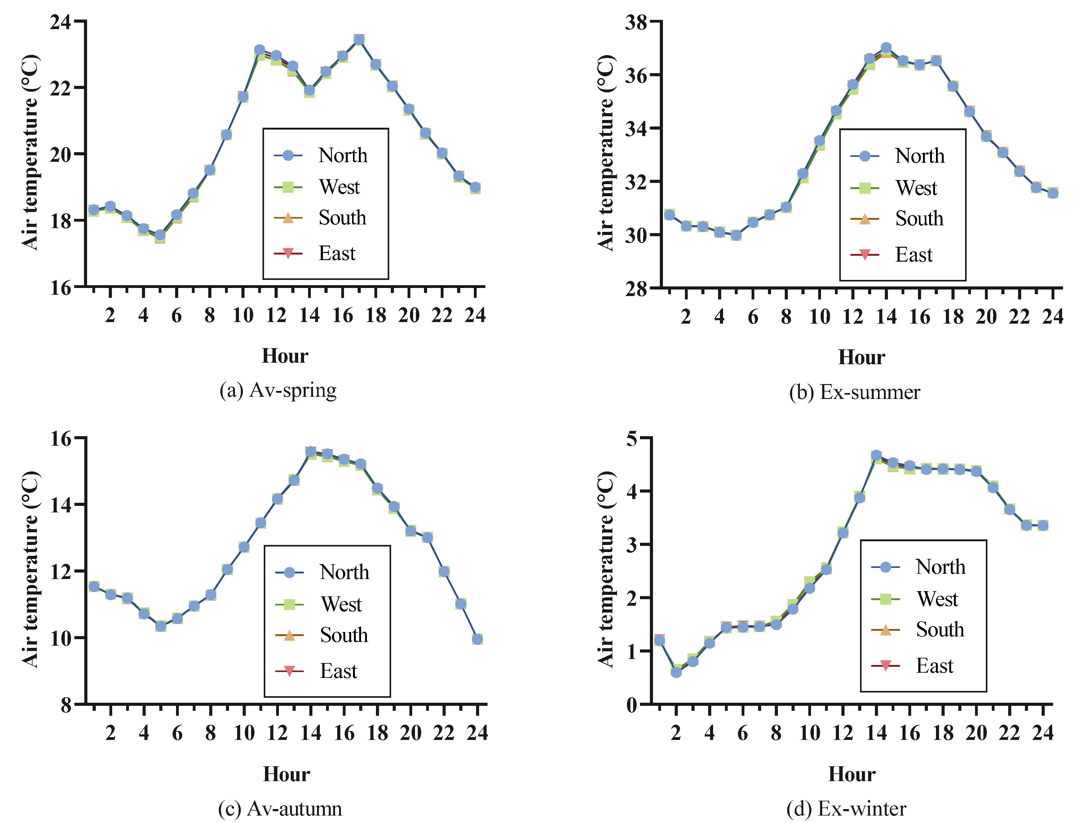
4.1. Microclimate Simulation Results
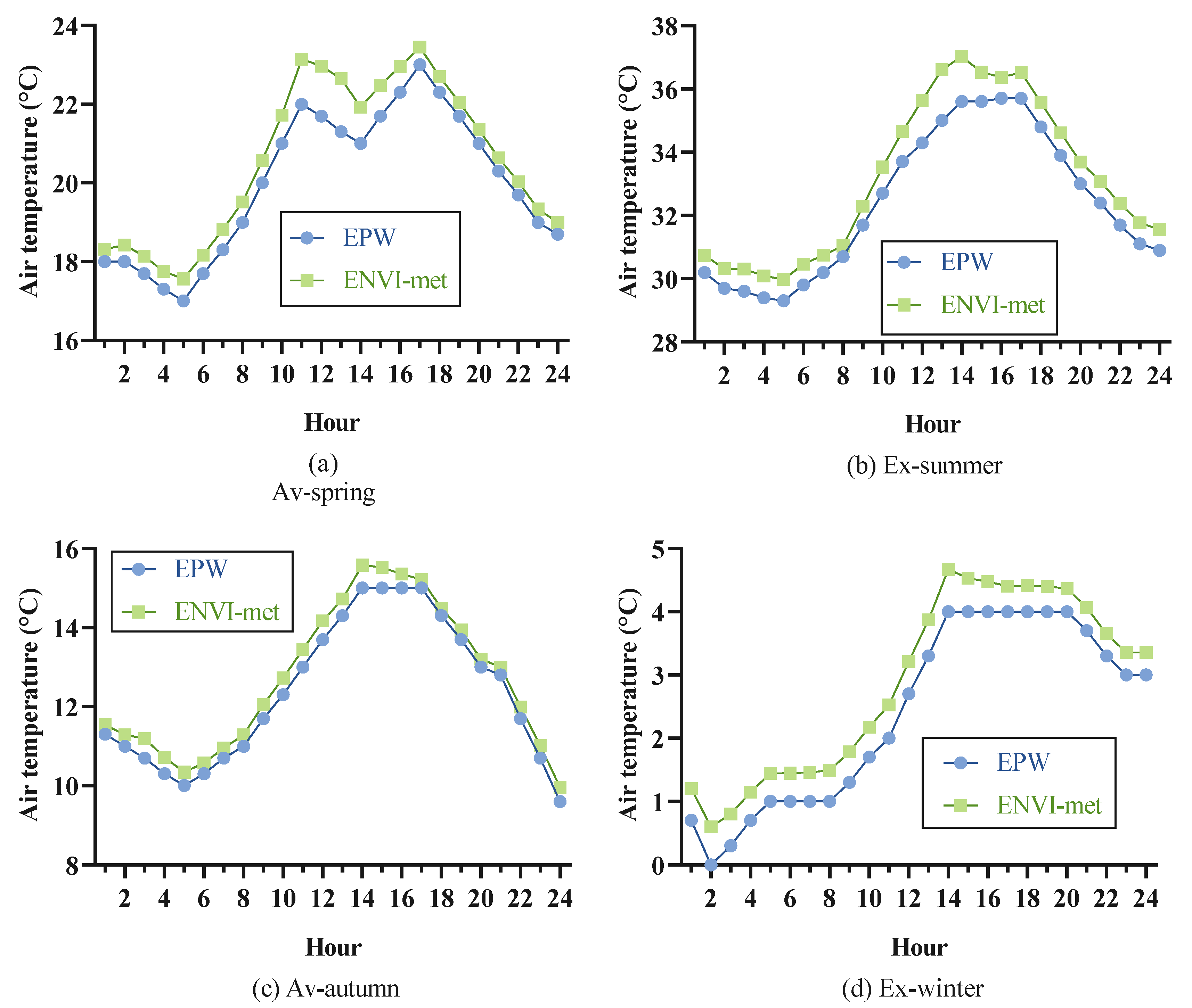
4.2. UHI Results for the Four Representative Days
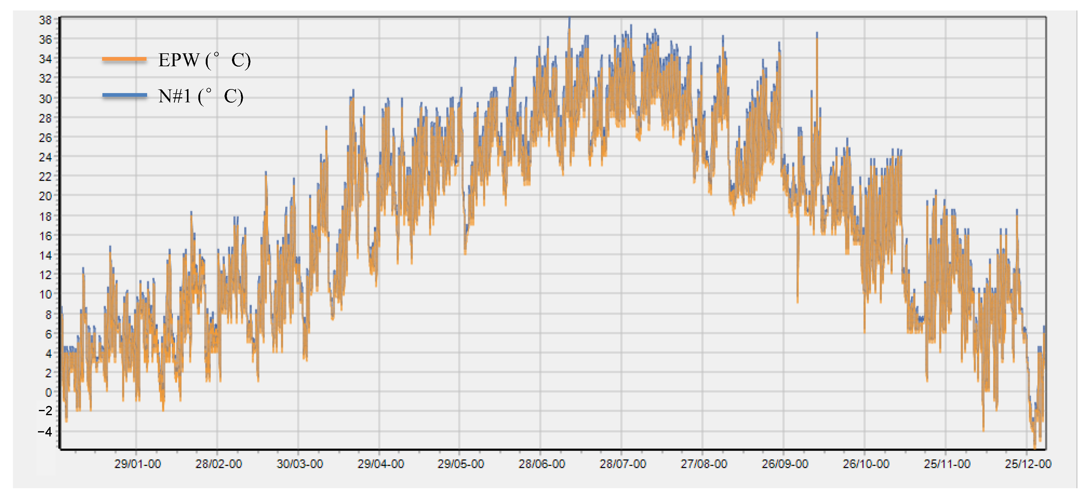
4.3. Generated Weather Files for COMFIE
4.4. Building Energy Simulation Results
4.4.1. DBES with Detailed Microclimate Data
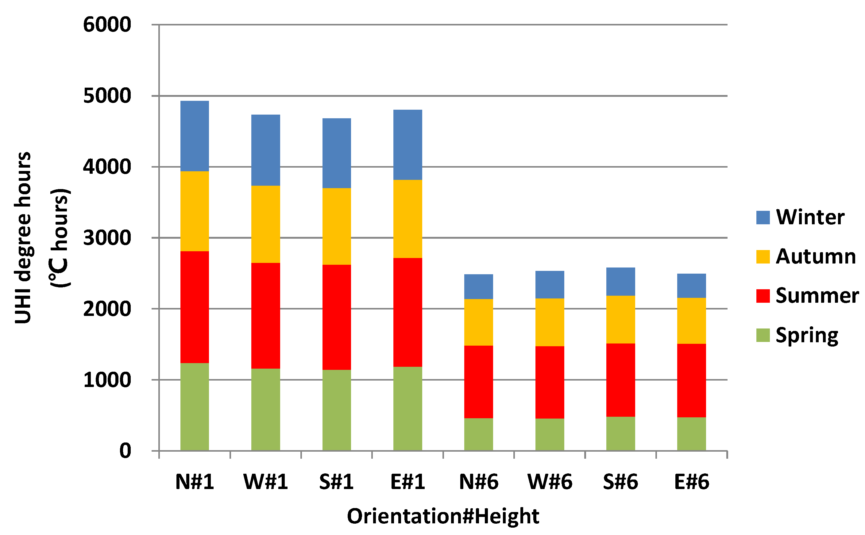
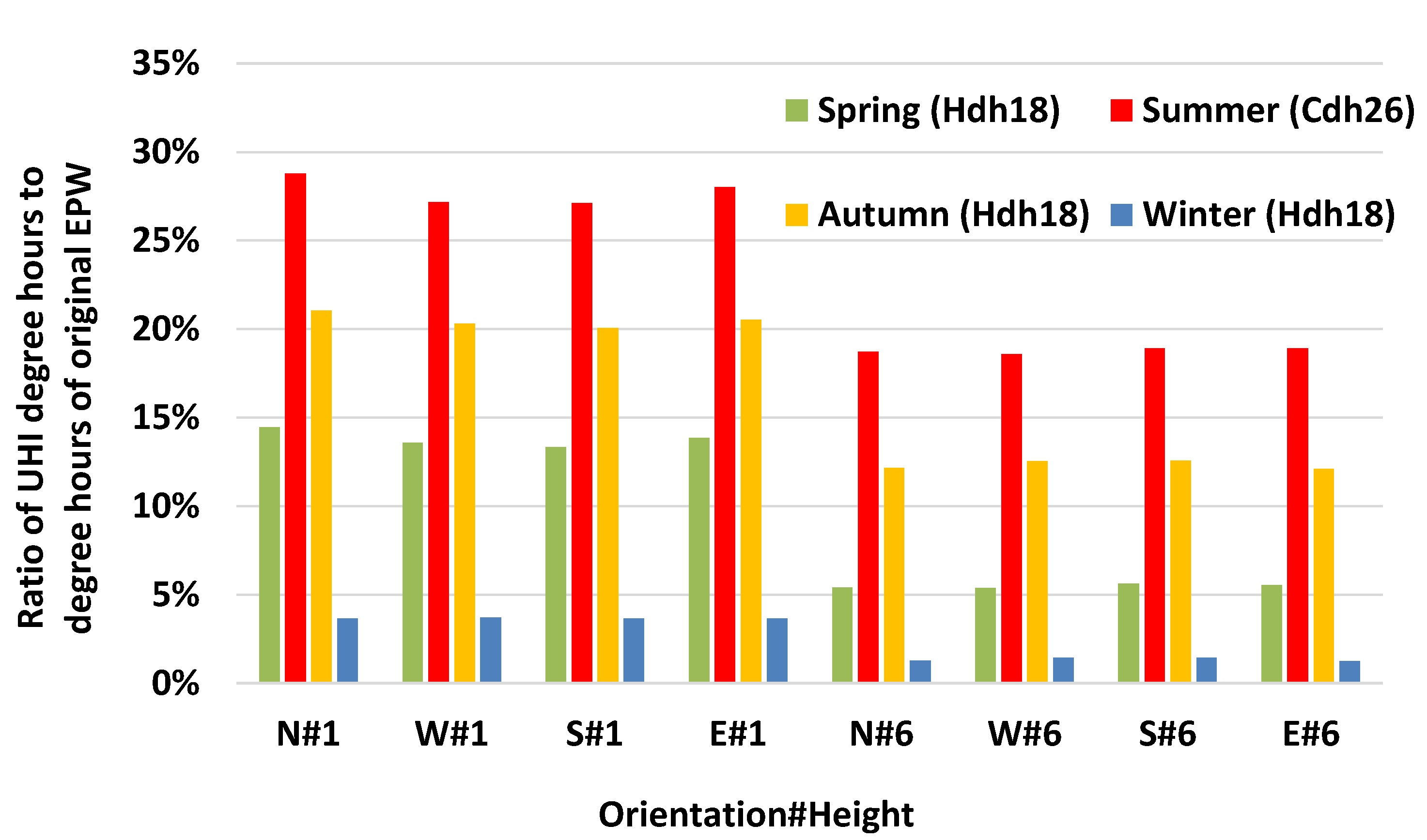
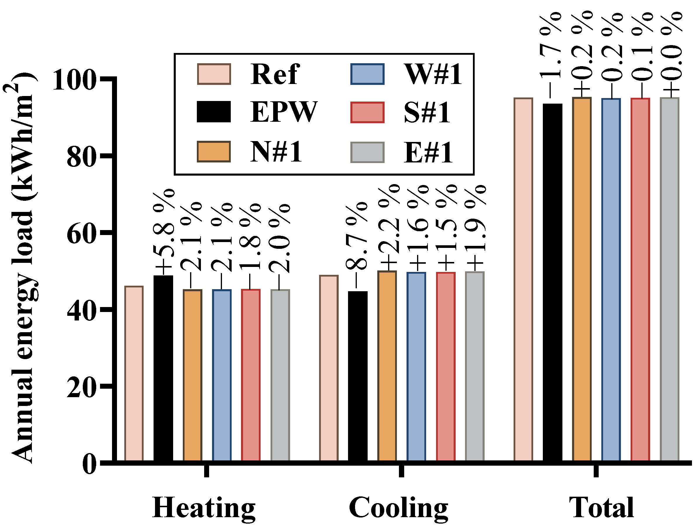
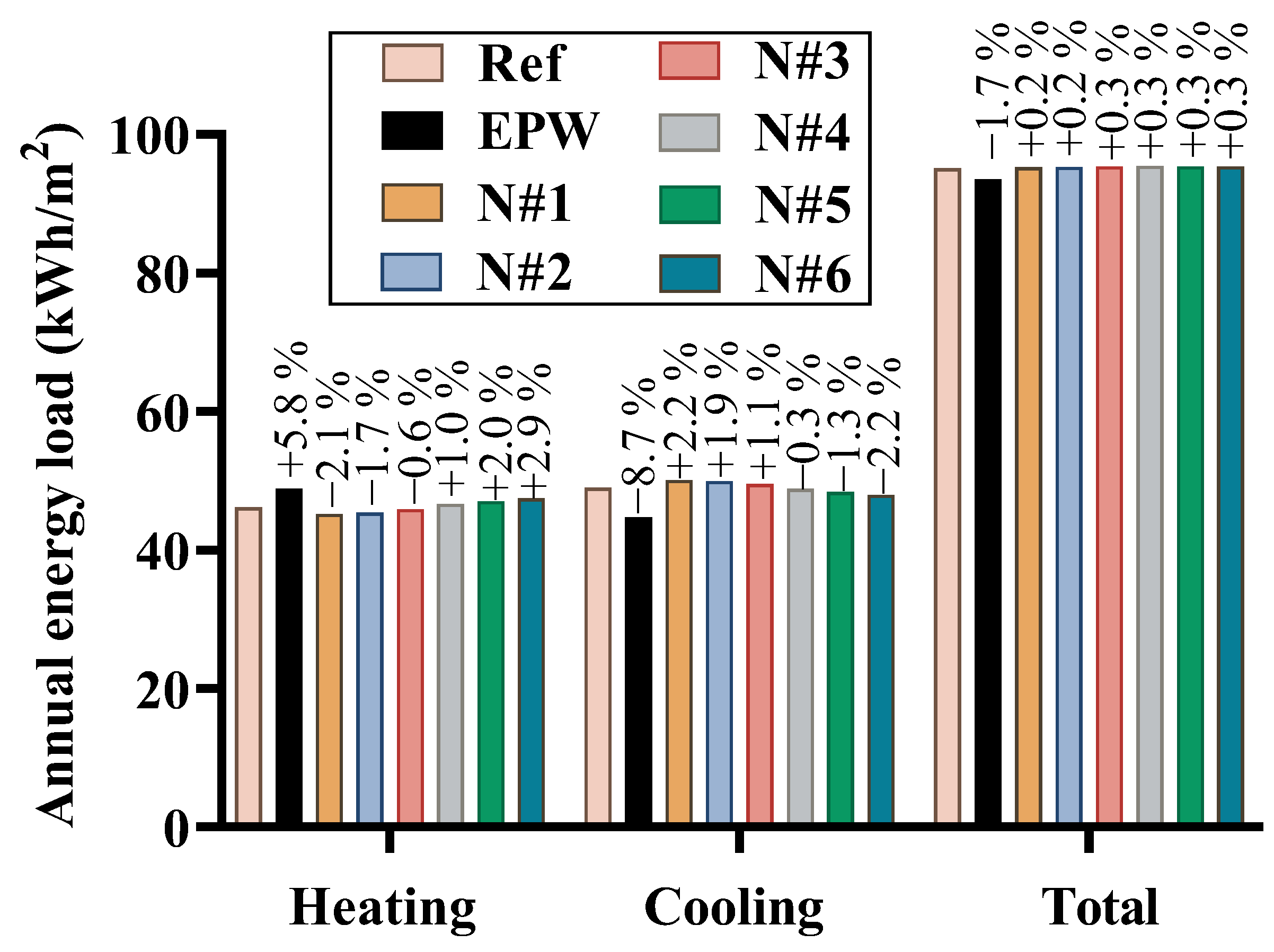
4.4.2. Impact of Orientation and Height
4.5. Discussion
5. Conclusions
Author Contributions
Funding
Institutional Review Board Statement
Data Availability Statement
Acknowledgments
Conflicts of Interest
Abbreviations
| List of abbreviations | |
| 3D | Three-dimensional |
| ach | air change per hour |
| DBES | Dynamic building energy simulation |
| E | East |
| EPW | EnergyPlus Weather |
| HSJG | Haishan Jingu |
| MAE | Mean absolute error |
| N | North |
| RMSE | Root mean square error |
| S | South |
| TMM | Typical meteorological months |
| TMY | Typical meteorological year |
| UCI | Urban cool island |
| UCII | Urban cool island intensity |
| UHI | Urban heat island |
| UHII | Urban heat island intensity |
| W | West |
| List of symbols | |
| I | Number of cells on x-axis in ENVI-met model |
| i | Hour number in a day |
| J | Number of cells on y-axis in ENVI-met model |
| j | Day number in a representative week |
| K | Number of cells on z-axis in ENVI-met model |
| k | Day number in a year |
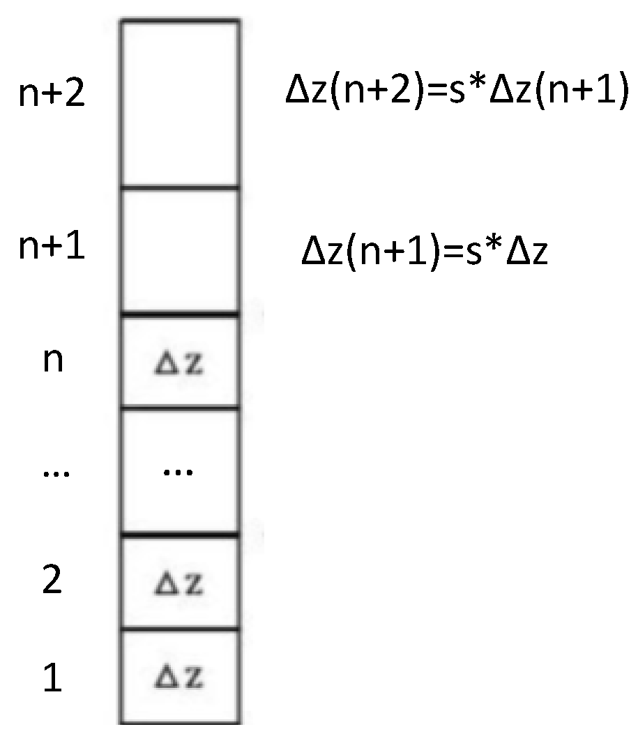
| n | Number of vertical cell |
| Nh | Number of different heights |
| P | Atmosphere pressure, Pa |
| P0 | Reference pressure, Pa |
| s | Scaling factor |
| T | Temperature, °C or K |
| UHIdh | Urban heat island degree-hours, °C hours |
| Superscripts and subscripts | |
| abs | Absolute |
| air | Air |
| av | Average |
| ENVImet | ENVI-met results |
| EPW | EPW file |
| max | Maximal |
| pot | Potential temperature |
| re1 | 1st representative day |
| re2 | 2nd representative day |
| List of Greek letters | |
| Δx | Resolution of cell on x-axis in ENVI-met model, m |
| Δy | The resolution of cell on y-axis in ENVI-met model, m |
| Δz | The resolution of cell on z-axis in ENVI-met model, m |
References
- Sun, Y.; Haghighat, F.; Fung, B.C.M. A Review of The-State-of-the-Art in Data-Driven Approaches for Building Energy Prediction. Energy Build. 2020, 221, 110022. [Google Scholar] [CrossRef]
- Tsoka, S.; Tolika, K.; Theodosiou, T.; Tsikaloudaki, K.; Bikas, D. A Method to Account for the Urban Microclimate on the Creation of ‘Typical Weather Year’ Datasets for Building Energy Simulation, Using Stochastically Generated Data. Energy Build. 2018, 165, 270–283. [Google Scholar] [CrossRef]
- Hall, I.J.; Prairie, R.R.; Anderson, H.E.; Boes, E.C. Generation of a Typical Meteorological Year; Sandia Labs.: Albuquerque, NM, USA, 1978. [Google Scholar]
- Wei, Y.; Huang, C.; Li, J.; Xie, L. An Evaluation Model for Urban Carrying Capacity: A Case Study of China’s Mega-Cities. Habitat Int. 2016, 53, 87–96. [Google Scholar] [CrossRef]
- Maheshwari, B.; Pinto, U.; Akbar, S.; Fahey, P. Is Urbanisation Also the Culprit of Climate Change?—Evidence from Australian Cities. Urban Clim. 2020, 31, 100581. [Google Scholar] [CrossRef]
- Toparlar, Y.; Blocken, B.; Maiheu, B.; van Heijst, G.J.F. Impact of Urban Microclimate on Summertime Building Cooling Demand: A Parametric Analysis for Antwerp, Belgium. Appl. Energy 2018, 228, 852–872. [Google Scholar] [CrossRef]
- Li, C.; Zhou, J.; Cao, Y.; Zhong, J.; Liu, Y.; Kang, C.; Tan, Y. Interaction between Urban Microclimate and Electric Air-Conditioning Energy Consumption during High Temperature Season. Appl. Energy 2014, 117, 149–156. [Google Scholar] [CrossRef]
- Oke, T.R. The Energetic Basis of the Urban Heat Island (Symons Memorial Lecture, 20 May 1980). Q. J. R. Meteorol. Soc. 1982, 108, 1–24. [Google Scholar]
- Imhoff, M.L.; Zhang, P.; Wolfe, R.E.; Bounoua, L. Remote Sensing of the Urban Heat Island Effect across Biomes in the Continental USA. Remote Sens. Environ. 2010, 114, 504–513. [Google Scholar] [CrossRef] [Green Version]
- Santamouris, M. Analyzing the Heat Island Magnitude and Characteristics in One Hundred Asian and Australian Cities and Regions. Sci. Total Environ. 2015, 512–513, 582–598. [Google Scholar] [CrossRef]
- Zhou, W.; Wang, J.; Cadenasso, M.L. Effects of the Spatial Configuration of Trees on Urban Heat Mitigation: A Comparative Study. Remote Sens. Environ. 2017, 195, 1–12. [Google Scholar] [CrossRef]
- Li, X.; Zhou, Y.; Asrar, G.R.; Imhoff, M.; Li, X. The Surface Urban Heat Island Response to Urban Expansion: A Panel Analysis for the Conterminous United States. Sci. Total Environ. 2017, 605–606, 426–435. [Google Scholar] [CrossRef] [PubMed]
- Li, H.; Zhou, Y.; Li, X.; Meng, L.; Wang, X.; Wu, S.; Sodoudi, S. A New Method to Quantify Surface Urban Heat Island Intensity. Sci. Total Environ. 2018, 624, 262–272. [Google Scholar] [CrossRef] [PubMed]
- Yang, X.; Peng, L.L.H.; Jiang, Z.; Chen, Y.; Yao, L.; He, Y.; Xu, T. Impact of Urban Heat Island on Energy Demand in Buildings: Local Climate Zones in Nanjing. Appl. Energy 2020, 260, 114279. [Google Scholar] [CrossRef]
- Tejedor, B.; Lucchi, E.; Nardi, I. Application of Qualitative and Quantitative Infrared Thermography at Urban Level: Potential and Limitations. In New Technologies in Building and Construction: Towards Sustainable Development; Bienvenido-Huertas, D., Moyano-Campos, J., Eds.; Lecture Notes in Civil Engineering; Springer Nature: Singapore, 2022; pp. 3–19. ISBN 978-981-19189-4-0. [Google Scholar]
- Martin, M.; Chong, A.; Biljecki, F.; Miller, C. Infrared Thermography in the Built Environment: A Multi-Scale Review. Renew. Sustain. Energy Rev. 2022, 165, 112540. [Google Scholar] [CrossRef]
- Lagüela, S.; Díaz−Vilariño, L.; Roca, D.; Lorenzo, H. Aerial Thermography from Low-Cost UAV for the Generation of Thermographic Digital Terrain Models. Opto-Electron. Rev. 2015, 23, 78–84. [Google Scholar] [CrossRef]
- Fabbri, K.; Costanzo, V. Drone-Assisted Infrared Thermography for Calibration of Outdoor Microclimate Simulation Models. Sustain. Cities Soc. 2020, 52, 101855. [Google Scholar] [CrossRef]
- Cho, Y.-I.; Yoon, D.; Shin, J.; Lee, M.-J. Comparative analysis of the effects of heat island reduction techniques in urban heatwave areas using drones. Korean J. Remote Sens. 2021, 37, 1985–1999. [Google Scholar] [CrossRef]
- Li, X.; Zhou, Y.; Yu, S.; Jia, G.; Li, H.; Li, W. Urban Heat Island Impacts on Building Energy Consumption: A Review of Approaches and Findings. Energy 2019, 174, 407–419. [Google Scholar] [CrossRef]
- Sun, Y.; Augenbroe, G. Urban Heat Island Effect on Energy Application Studies of Office Buildings. Energy Build. 2014, 77, 171–179. [Google Scholar] [CrossRef]
- Skelhorn, C.P.; Levermore, G.; Lindley, S.J. Impacts on Cooling Energy Consumption Due to the UHI and Vegetation Changes in Manchester, UK. Energy Build. 2016, 122, 150–159. [Google Scholar] [CrossRef] [Green Version]
- Lowe, S.A. An Energy and Mortality Impact Assessment of the Urban Heat Island in the US. Environ. Impact Assess. Rev. 2016, 56, 139–144. [Google Scholar] [CrossRef]
- Bruse, M.; Fleer, H. Simulating Surface–Plant–Air Interactions inside Urban Environments with a Three Dimensional Numerical Model. Environ. Model. Softw. 1998, 13, 373–384. [Google Scholar] [CrossRef]
- Huttner, S. Further Development and Application Ofthe 3D Microclimate Simulation ENVI-Met. Ph.D. Thesis, Johannes Gutenberg University Mainz, Mainz, Germany, 2012. [Google Scholar]
- López-Cabeza, V.P.; Galán-Marín, C.; Rivera-Gómez, C.; Roa-Fernández, J. Courtyard Microclimate ENVI-Met Outputs Deviation from the Experimental Data. Build. Environ. 2018, 144, 129–141. [Google Scholar] [CrossRef]
- Ayyad, Y.; Sharples, S. Envi-MET Validation and Sensitivity Analysis Using Field Measurements in a Hot Arid Climate. In Proceedings of the IOP Conference Series: Earth and Environmental Science, Cardiff, Wales, 24–25 September 2019; Volume 329, p. 012040. [Google Scholar] [CrossRef] [Green Version]
- Elwy, I.; Ibrahim, Y.; Fahmy, M.; Mahdy, M. Outdoor Microclimatic Validation for Hybrid Simulation Workflow in Hot Arid Climates against ENVI-Met and Field Measurements. Energy Procedia 2018, 153, 29–34. [Google Scholar] [CrossRef]
- Sharmin, T.; Steemers, K. Understanding ENVI-Met (V4) Model Behaviour in Relation to Environmental Variables. In Proceedings of the PLEA 2017 Edinburgh: Design to Thrive, Edinburgh, UK, 2 July 2017; pp. 2156–2164. [Google Scholar]
- Yang, X.; Zhao, L.; Bruse, M.; Meng, Q. Evaluation of a Microclimate Model for Predicting the Thermal Behavior of Different Ground Surfaces. Build. Environ. 2013, 60, 93–104. [Google Scholar] [CrossRef]
- Peuportier, B.; Blanc-Sommereux, I. Simulation Tool with Its Expert Interface for the Thermal Design of Multizone Buildings. Int. J. Sol. Energy 1990, 8, 109–120. [Google Scholar] [CrossRef]
- Peuportier, B. COMFIE, Logiciel Pour L’architecture Bioclimatique, Quelques Applications Pour Les Vérandas; Journée Technique GENEC (CEA): Marseille, France, 1993. [Google Scholar]
- Peuportier, B. Bancs D’essais de Logiciels de Simulation Thermique. In Proceedings of the Journée Thématique IBPSA France—SFT 2005, Outil de Simulation Thermo-Aéraulique du Bâtiment, La Rochelle, France, 31 March 2005. [Google Scholar]
- Brun, A.; Spitz, C.; Wurtz, E.; Mora, L. Behavioural Comparison of Some Predictive Tools Used in a Low-Energy Building. In Proceedings of the Eleventh International IBPSA Conference, Glasgow, Scotland, 27–30 July 2009. [Google Scholar]
- Recht, T.; Munaretto, F.; Schalbart, P.; Peuportier, B. Analyse de la Fiabilité de COMFIE par Comparaison à Des Mesures. Application à un Bâtiment Passif. In Proceedings of the Conférence IBPSA France-Arras-2014, Arras, France, 20 May 2014; p. 8. [Google Scholar]
- Spitz, C. Analyse de la Fiabilite Des Outils de Simulation et Des Incertitudes de Métrologie Appliquée à L’efficacité Energétique Des Bâtiments. Ph.D. Thesis, Université de Grenoble, Grenoble, France, 2012. [Google Scholar]
- Pei, L. The Study on Eco-Design of High-Rise Residential Buildings in Wuhan Based on Energy Simulation and Life Cycle Assessment. Master’s Thesis, Huazhong University of Science & Technology, Wuhan, China, 2015. [Google Scholar]
- EnergyPlus. Available online: https://energyplus.net/weather-location/asia_wmo_region_2/CHN/CHN_Hubei.Wuhan.574940_SWERA (accessed on 21 February 2023).
- Yang, X.; Yao, L.; Peng, L.L.H.; Jiang, Z.; Jin, T.; Zhao, L. Evaluation of a Diagnostic Equation for the Daily Maximum Urban Heat Island Intensity and Its Application to Building Energy Simulations. Energy Build. 2019, 193, 160–173. [Google Scholar] [CrossRef]
- Lauzet, N.; Rodler, A.; Musy, M.; Azam, M.-H.; Guernouti, S.; Mauree, D.; Colinart, T. How Building Energy Models Take the Local Climate into Account in an Urban Context—A Review. Renew. Sustain. Energy Rev. 2019, 116, 109390. [Google Scholar] [CrossRef]
- Thiers, S. Bilans Energétiques et Environnementaux de Bâtiments à Energie Positive. Ph.D. Thesis, École Nationale Supérieure des Mines de Paris, Paris, France, 2008. [Google Scholar]
- Wu, N.; Shi, P.; Zhu, G.; Pan, X. Changes of soil relative moisture content and influencing factor in the yangtze basin during 1992–2012. Resour. Environ. Yangtze Basin 2017, 26, 1001–1010. [Google Scholar] [CrossRef]
- Ministry of Housing and Urban-Rural Development. Design Standard for Energy Efficiency of Residential Buildings in Hot Summer and Cold Winter Zone; China Architecture & Building Press: Beijing, China, 2010.
- Yang, X.; Yao, L.; Jin, T.; Peng, L.L.H.; Jiang, Z.; Hu, Z.; Ye, Y. Assessing the Thermal Behavior of Different Local Climate Zones in the Nanjing Metropolis, China. Build. Environ. 2018, 137, 171–184. [Google Scholar] [CrossRef]
- Huang, K.-T.; Li, Y.-J. Impact of Street Canyon Typology on Building’s Peak Cooling Energy Demand: A Parametric Analysis Using Orthogonal Experiment. Energy Build. 2017, 154, 448–464. [Google Scholar] [CrossRef]
- Chan, A.L.S. Developing a Modified Typical Meteorological Year Weather File for Hong Kong Taking into Account the Urban Heat Island Effect. Build. Environ. 2011, 46, 2434–2441. [Google Scholar] [CrossRef]
- Peters, J.F.; Iribarren, D.; Juez Martel, P.; Burguillo, M. Hourly Marginal Electricity Mixes and Their Relevance for Assessing the Environmental Performance of Installations with Variable Load or Power. Sci. Total Environ. 2022, 843, 156963. [Google Scholar] [CrossRef] [PubMed]


| Season | Representative Week (Directly from EnergyPlus Website) | Representative Day | Abbreviation | RMSE (°C) | MAE (°C) |
|---|---|---|---|---|---|
| Summer Extreme hot | 5–11 August | 9 August | Ex-summer | 0.82 | 0.76 |
| Winter Extreme cold | 1–7 January | 4 January | Ex-winter | 1.11 | 0.90 |
| Spring Average temperature | 27 May–2 June | 2 June (date is in June, but represents spring) | Av-spring | 1.48 | 1.19 |
| Autumn Average temperature | 26 November–2 December | 30 November | Av-autumn | 1.25 | 1.02 |
| Sidewalk | Built Area | Green Space | Asphalt Concrete Road |
|---|---|---|---|
| Brick: 0~3 cm | Concrete: 0~20 cm | Sandy loam: 0~40 cm | Asphalt concrete: 0~10 cm |
| Concrete: 4~20 cm | Sand: 21~ 30 cm | Loam: 41~450 cm | Sand: 11~40 cm |
| Sand: 21~30 cm | Loam: 31~450 cm | Loam: 41~450 cm | |
| Loam: 31~450 cm |
| Av-Spring | Ex-Summer | Av-Autumn | Ex-Winter | |
|---|---|---|---|---|
| Upper layer (0–20 cm) | 26 °C/77% | 33.51 °C/85% | 12.33 °C/84% | 6.16 °C/80.5% |
| Middle layer (20–50 cm) | 24.66 °C/80.5% | 32.57 °C/81% | 13.66 °C/83% | 7.53 °C/83% |
| Deep layer (50–200 cm) | 21.07 °C/82% | 29.30 °C/79% | 17.20 °C/81% | 11.65 °C/84% |
| Bedrock layer (below 200 cm) | 19 °C/82% | 19 °C/79% | 19 °C/81% | 19 °C/84% |
| External Wall | Roof |
|---|---|
| Ceramic tile 1 cm | Ceramic tile 1 cm |
| Insulation mortar 4 cm | Extruded Polystyrene Board (XPS) 4 cm |
| Aerated concrete block 20 cm | Concrete (C10) 20 cm |
| Building Level | Level Height | Weather File Abbreviation of Four Orientations at Each Height | Height of the Weather File by Averaging the Heights of Vertical Cells in ENVI-met |
|---|---|---|---|
| 1 | 3 m | N#1, W#1, S#1, E#1 | 3 m (cell 1) |
| 2–6 | 6–18 m | N#2, W#2, S#2, E#2 | (9 m (cell 2)+ 15 m (cell 3))/2 = 12 m |
| 7–14 | 21–42 m | N#3, W#3, S#3, E#3 | (21 m (cell 4) + 27 m (cell 5) + 33.75 m (cell 6) + 42.19 m (cell 7))/4 = 31 m |
| 15–25 | 45–75 m | N#4, W#4, S#4, E#4 | (52.73 m (cell 8) + 65.92 m (cell 9))/2 = 59.3 m |
| 26–33 | 78–99 m | N#5, W#5, S#5, E#5 | 82.4 m (cell 10) |
| 34 | 102 m | N#6, W#6, S#6, E#6 | 103 m (cell 11) |
| Zone Number | Zone Name | Weather File |
|---|---|---|
| 1 | floor 1 | (N#1 + S#1 + W#1 + E#1)/4 |
| 2 | aisle | - |
| 3 | floor 2–6 north | (N#2 + S#2 + W#2 + E#2)/4 |
| 4 | floor 2–6 south | S#2 |
| 5 | floor 7–14 north | (N#3 + S#3 + W#3 + E#3)/4 |
| 6 | floor 7–14 south | S#3 |
| 7 | floor 15 C—living room (15) | S#4 |
| 8 | floor 15 C—bedroom (15) | S#4 |
| 9 | floor 15 C—other rooms (15) | S#4 |
| 10 | floor 15 B | S#4 |
| 11 | floor 15 north | (N#4 + S#4 + W#4 + E#4)/4 |
| 12 | floor 16–25 north | (N#4 + S#4 + W#4 + E#4)/4 |
| 13 | floor 16–25 south | S#4 |
| 14 | floor 26–33 north | (N#5 + S#5 + W#5 + E#5)/4 |
| 15 | floor 26–33 south | S#5 |
| 16 | floor 34 north | (N#6 + S#6 + W#6 + E#6)/4 |
| 17 | floor 34 south | S#6 |
| Representative Day | UHIImax (°C) | UHIIav (°C) |
|---|---|---|
| Av-spring | 1.35 | 0.58 |
| Ex-summer | 1.61 | 0.78 |
| Av-autumn | 0.58 | 0.34 |
| Ex-winter | 0.67 | 0.47 |
Disclaimer/Publisher’s Note: The statements, opinions and data contained in all publications are solely those of the individual author(s) and contributor(s) and not of MDPI and/or the editor(s). MDPI and/or the editor(s) disclaim responsibility for any injury to people or property resulting from any ideas, methods, instructions or products referred to in the content. |
© 2023 by the authors. Licensee MDPI, Basel, Switzerland. This article is an open access article distributed under the terms and conditions of the Creative Commons Attribution (CC BY) license (https://creativecommons.org/licenses/by/4.0/).
Share and Cite
Pei, L.; Schalbart, P.; Peuportier, B. Quantitative Evaluation of the Effects of Heat Island on Building Energy Simulation: A Case Study in Wuhan, China. Energies 2023, 16, 3032. https://doi.org/10.3390/en16073032
Pei L, Schalbart P, Peuportier B. Quantitative Evaluation of the Effects of Heat Island on Building Energy Simulation: A Case Study in Wuhan, China. Energies. 2023; 16(7):3032. https://doi.org/10.3390/en16073032
Chicago/Turabian StylePei, Long, Patrick Schalbart, and Bruno Peuportier. 2023. "Quantitative Evaluation of the Effects of Heat Island on Building Energy Simulation: A Case Study in Wuhan, China" Energies 16, no. 7: 3032. https://doi.org/10.3390/en16073032