Article

Dynamic Equivalent Model Considering Multiple Induction Motors for System Frequency Response

1
State Grid Shanxi Electric Power Research Institute, Taiyuan 030001, China
2
Dispatch and Control Center, State Grid Shanxi Electric Power Company, Taiyuan 030021, China
3
School of Electric Engineering, Xi’an Jiaotong University, Xi’an 710049, China
*
Author to whom correspondence should be addressed.
Energies 2023, 16(7), 2987; https://doi.org/10.3390/en16072987
Submission received: 13 February 2023 / Revised: 14 March 2023 / Accepted: 20 March 2023 / Published: 24 March 2023
(This article belongs to the Topic Advanced Systems Engineering: Theory and Applications)

Abstract

:
Renewable energy sources have been characterized by a persistent and rapid proliferation, which has resulted in a notable reduction in grid inertia over an extended period. There is a widely held belief that the primary source of inertia within the grid stems from generation-side conventional units. However, in power consumption, a significant number of induction motors are present, which can inherently offer rotational inertia by virtue of their kinetic energy. To investigate the influence of induction motors on grid inertia, in this paper, we propose two types of models, i.e., a detailed grid model and a dynamic equivalent model that considers multiple induction motors. Specifically, the detailed grid model with multiple induction motors is first established. However, the detailed model requires the specific parameters of induction motors, which are hard to acquire in large systems. Moreover, the accuracy of the model is unsatisfactory. To fill these gaps, the dynamic equivalent model (DEM) is further proposed to emulate the detailed model. Compared with the detailed model, the proposed dynamic equivalent model is structurally simple and does not require the specific parameters of induction motors. Therefore, it is possible to apply to large systems for investigating the influence of induction motors on grid frequency dynamics. A genetic algorithm is introduced in order to figure out the parameters of the proposed dynamic equivalent model from historical frequency data. The proposed detailed model and dynamic equivalent model are evaluated on the IEEE 9-bus system in MATLAB and SimPowerSystems toolbox.

1. Introduction

As the combustion of fossil fuels continues to rise, countries worldwide are confronted with the dual pressures of energy requirements and environmental preservation, prompting a heightened focus on renewable energy as a solution to these pressing global issues [1,2]. Among all the renewable energy resources, wind energy and solar energy have attracted the most attention due to their advantages, such as wide distribution of resources, mature key technologies, short construction cycle, and pollution-free characteristics [3,4,5,6]. According to the Global Wind Energy Council (GWEC), global wind power generation capacity experienced an addition of 93.6 GW in 2021. Moreover, the worldwide cumulative wind power capacity reached 837 GW with the installation of new wind power in 2021, representing an annual growth rate of 12% [7]. From this point of view, it is expected that there will be a consistent and accelerated expansion of renewable energy [8].
To make the most of the renewable energy resources, voltage source converters (VSCs) are introduced into the energy conversion systems [9,10,11,12]. As an intuitive example, Figure 1 presents a typical wind energy conversion system (WECS). From this figure, it can be seen that the permanent magnet synchronous generator (PMSG)-based wind turbine is connected to the grid through two VSCs, i.e., a rotor-side converter (RSC) and a grid-side converter (GSC). These converters decouple the rotor speed of the wind turbine from the grid frequency, thus reducing the grid inertia and posing a risk to the stable operation of the power system.
Given the significance of frequency stability in power systems, it is unsurprising that research efforts have predominantly centered on grid inertia. Currently, the literature about grid inertia mainly focuses on the inertia of conventional generating units and renewable energy generating units [13,14,15,16]. Specifically, conventional generating units such as a thermal generating unit and a hydroelectric generating unit, are connected to the grid directly. Therefore, when the grid frequency decreases (or increases), the rotor speed of the conventional generating unit decelerates (or accelerates). Correspondingly, the kinetic energy stored in the rotating rotor is naturally used to provide inertial support. When it comes to renewable energy generating units, there is a widely held belief that they make no contribution to the grid inertia. The reason is that these renewable energy generating units are connected to the grid through VSCs, thus they are decoupled from the grid. However, with the proper design of an additional inertia support controller, renewable energy generating units can provide inertia support to the grid, thus increasing grid inertia [17,18,19,20]. Specifically, in addition to generation-side units, there are a considerable amount of induction motors on the consumption-side, as shown in Figure 2. These induction motors can also contribute to grid inertia due to their stored kinetic energy. In a power system with a high penetration of renewable energy, the influence of induction motors on grid inertia becomes more prominent.
To the best of our knowledge, only few studies have addressed the impact of induction motors on grid inertia [21,22,23]. In [21], Zhou et al. established the induction motor model during the frequency regulation process and derived its transfer function by linearizing the relationship between active power and induction motor slip. Furthermore, in [22], Chen et al. formulated the induction model as a proportionate decrease in electromagnetic power with respect to the frequency deviation. In [23], from the viewpoint of power balance, Wang et al. constructed a model of the induction motor in the electromechanical transient process and presented a voltage magnitude-phase dynamic analysis. Although these studies revealed that consumption-side induction motors in a grid do affect grid inertia, they shared a common limitation, that is, only one aggregated induction motor was considered. On the one hand, it is hard to obtain the parameters of the aggregated induction motors in practice. On the other hand, induction motors operate at different operating points and using one aggregated model may introduce errors. From this point of view, there is still a lack of research on the grid frequency response model that considers multiple induction motors.
In addition to the grid frequency response model that considers multiple induction motors, it remains a challenge to apply the model in practice due to its complex structure and the requirements of the specific parameters of induction motors. As a result, the dynamic equivalent model (DEM) is urgently needed to reduce computation efforts while ensuring calculation accuracy. This can be achieved using the data-driven approach [24,25,26,27]. In fact, the data-driven approach has been widely used in studying power systems. In [24], to develop the dynamic equivalent model, Hu et al. presented a data-driven inertial response identification algorithm (IRIA). With this algorithm, the inertial support of the wind farm was emulated. Moreover, the inertia constant of the wind farm is further identified based on the grid frequency and wind farm power output. In [25], based on the data-driven method, Liu et al. presented a power flow linearization approach. This data-driven-based method can simplify and accelerate the calculation of a power system’s control, operation, and optimization. In Zheng et al. [26], an electricity theft detection approach was developed based on the data-driven method. By combining the clustering as well as the maximum information coefficient technique, the data-driven based approach can detect the electricity thefts in a faster and more accurate way. In Jiang et al. [27], a data-driven-based mode estimator was established for investigating inter-area oscillation which occurs in actual power systems. With this estimator, the inter-area oscillation mode in the China Southern Power Grid can be identified using phaser measurement units under both ring-down and ambient conditions. However, using the data-driven approach to develop the grid dynamic equivalent model to emulate the frequency dynamics of grid with multiple induction motors is rarely discussed.
From the above observations, we confront two main issues to investigate the influence of the induction motors on the inertia of a power system. The first issue is developing a grid frequency response model that considers multiple induction motors, while the second issue is reducing the complexity of the grid frequency response model while ensuring its calculation accuracy. To fill these gaps, in this work, firstly, a detailed grid model that considers multiple induction motors is established. Furthermore, considering the fact that the detailed model requires the specific parameters of induction motors, which are hard to acquire in large systems, a dynamic equivalent model is established to emulate the detailed one. Moreover, a data-driven method is introduced to figure out the parameters of the proposed dynamic equivalent model from historical frequency data. The proposed dynamic equivalent model is structurally simple and does not require specific parameters of induction motors compared with the detailed model. Therefore, it is possible to employ it in actual large systems.
The key contributions of the paper are threefold.
  • A detailed grid model incorporating multiple induction motors is established to imitate the influence of induction motors on grid inertia.
  • To address the limitations of the detailed grid model, a dynamic equivalent model is further proposed. Compared with the detailed model, the proposed dynamic equivalent model is structurally simple and does not require the specific parameters of induction motors. Thus, it is possible to apply it to large systems.
  • A genetic algorithm-based approach is introduced to identify the parameters of the dynamic equivalent model. Its optimality is guaranteed by an ad hoc approach.
The rest of the paper is organized as follows: Section 2 develops a detailed frequency response model considering multiple induction motors. Based on the detailed grid frequency response model, a dynamic equivalent model incorporating multiple induction motors is further derived using the genetic algorithm in Section 3. The proposed dynamic equivalent model is structurally simple and does not require the specific parameters of induction motors compared with the detailed model. In Section 4, the case studies are employed to evaluate performance of the detailed grid frequency response model and the dynamic equivalent model. Finally, a conclusion is drawn in Section 5.

2. Modeling of the Grid with Multiple Induction Motors

The detailed grid frequency response model incorporating multiple induction motors is developed in this section. With this detailed model, the influence of the induction motors on grid inertia can be investigated.
To derive the detailed model, firstly, a small signal model of introduction motors is proposed in the Laplace domain. Secondly, the above model is aggregated into the low-order system frequency response model. This aggregated model is exactly the detailed model of the grid that considers multiple induction motors. Compared with the current grid frequency response model, this detailed model includes not only the frequency response dynamics of the generating-side units, but also that of the multiple induction motors.

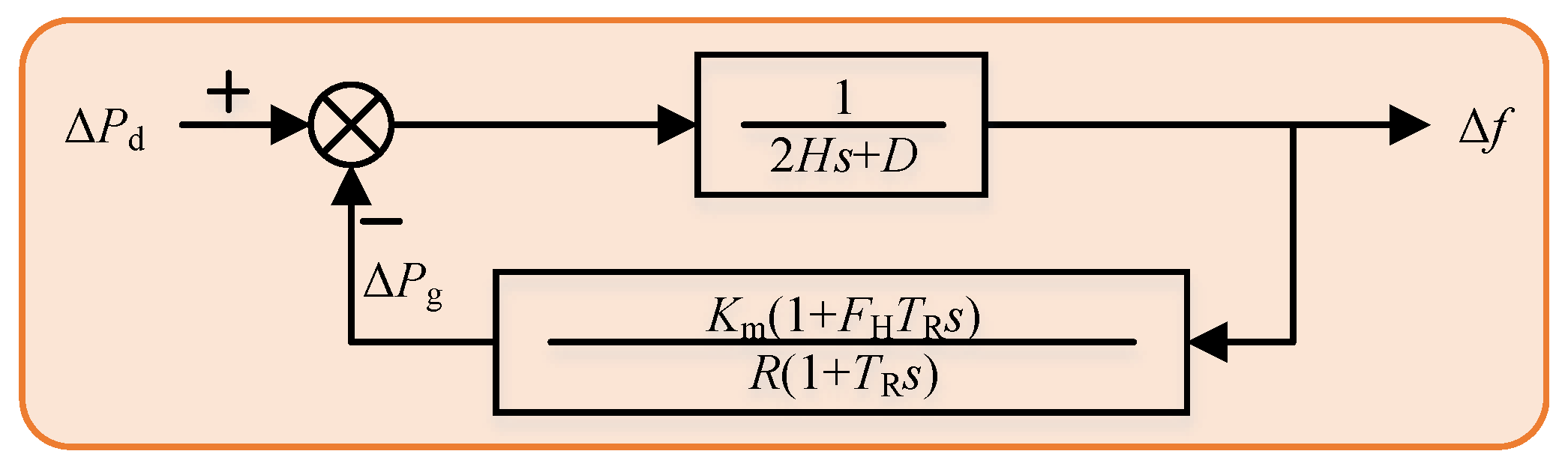
2.1. Low-Order System Frequency Response Model

The deviation of the utility grid frequency from its nominal value occurs once there is an active power imbalance between the grid load and generation. The low-order frequency response model of the grid, which is simple and fairly precise, can be employed to emulate this frequency behavior [28]. This low-order system frequency response model is capable of filtering out synchronizing oscillations between onshore conventional generation units, while still retaining the average frequency behavior. This low-order system model dynamics can be described as
d ( Δ f ) d t = D 2 H Δ f + 1 2 H ( Δ P d + Δ P g )
where Δ f denotes grid frequency deviation, H presents the grid inertia constant, usually within 3~9 s [29], D denotes the frequency damping coefficient of the utility grid, Δ P g represents the conventional generators’ power variation subsequent to the occurrence of a load disturbance, and Δ P d is grid load disturbance resulting from sudden load changes, either load increases or load decreases. In (1), the dynamics of Δ P g and Δ P d are [30]
Δ P d = P d , m · ε ( t t 0 )
d ( Δ P g ) d t = 1 T R · Δ P g + K m F H R · d ( Δ f ) d t + K m T R R · Δ f
Here, P d , m is the magnitude of the load disturbance in utility grid and ε ( t t 0 ) is the step signal indicating the occurrence of a load disturbance at time instant t 0 . The reheat time constant T R is a factor that predominantly influences the response of the majority of reheat turbine power output, typically within 6~14 s, K m is the mechanical power gain factor and it is subject to the influence of the system spinning reserve and power factor, while F H represents the high-pressure fraction of the turbine, usually within 0.15~0.4 [28], and R denotes governor speed regulation.
The Laplace domain representation can also be used to express the low-order system frequency response model (1)~(3), as shown in Figure 3.

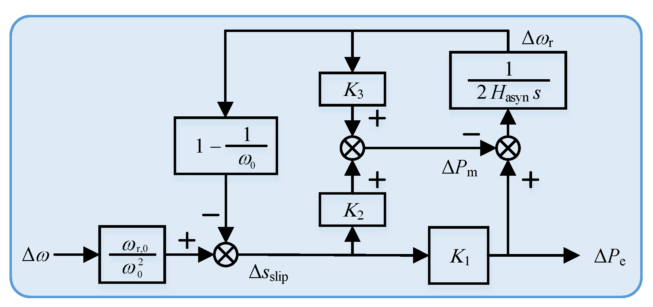
2.2. Induction Motor Model

In this subsection, the induction motor model will be derived. The influence of the induction motors on grid inertia can be further investigated with this model.
In general, grid inertia is mainly contributed by the synchronous generation units. Specifically, for the i-th synchronous generation unit in the utility grid, its inertia constant H s y n , i can be calculated as
H syn , i = E k , i S B , i = J i ( 2 π f m ) 2 2 S B , i
Here, E k , i is the rotational kinetic energy of i-th generation unit, J i denotes the inertia moment of i-th generation unit, f m represents the normal frequency of the utility grid, and S B , i denotes the rated power of i-th generation unit.
Once we obtain the inertia constants of all the synchronous generation units, the entire inertia of the grid can be derived as
H = i = 1 N H syn , i i = 1 N S B , i
Here, N is the number of generation units in the utility grid. From (5), it is clear that the inertia of the utility grid is contributed to by the synchronous generation units.
In fact, in addition to the synchronous generation units, there are a considerable amount of induction motors on the consumption-side, which can also contribute to grid inertia due to their stored kinetic energy. Traditionally, the frequency of the utility grid is mainly dominated by the inertial responses and the governor responses of the synchronous generation units, thus, the inertia of the grid is sufficient. As a result, the influence of the induction motors on grid inertia can be disregarded. However, the accelerated expansion of the renewable generation units results in a decreasing number of on-line synchronous generation units and, thus, reduces grid inertia significantly. In this scenario, the influence of the induction motor on grid inertia should be addressed. Moreover, it is necessary to investigate induction motors’ equivalent inertia.
In agreement with (4), of course, we can obtain the inertia of an induction motor, i.e., H asyn , as follows
H asyn = E k , asyn S B , asyn = J asyn ( 2 π f m ) 2 2 S B , asyn
However, H asyn cannot be aggregated into (5) directly because, compared with synchronous generation units, there is the slip between induction motors’ rotor speed and the grid frequency [23]. In other words, H asyn can only roughly, but not precisely, represent the influence of the induction motor on grid inertia. To fill this gap, a more precise equivalent inertia constant for induction motors should be developed.
From Figure 3, we can find that the grid inertia is relative with the deviation of power (i.e., Δ P d and Δ P g ) and grid frequency (i.e., Δ f ). Inspired by this observation, the relationship between the deviation of induction motor’s input active power (i.e., Δ P e ) and grid frequency (i.e., Δ f ) should be derived to precisely investigate the influence of the induction motor on the grid inertia.
To develop the relationship between Δ P e and Δ f , the dynamics of the induction motor should be established, as follows [21]
2 H asyn d ω r d t = P e P m
Here, ω r is the induction motor’s rotor speed, P e is the input electromagnetic power of induction motor, and P m is induction motor’s output mechanical power.
In (7), P e can be expressed as [23]
P e = U t 2 r s + r r s slip 2 + x s + x r 2 · r r s slip
Here, U t 2 is the stator voltage of induction motors, r s and r r are the stator and rotor resistance of the induction motor, x s and x r are the stator and rotor impedance of the induction motor, and s slip denotes the slip of induction motors, which can be described as
s slip = ω ω r ω
Here, ω is the rotating magnetic field speed of the stator.
Moreover, P m in (7) can be expressed as [21]
P m = ω r k α + ( 1 α ) 1 s slip ρ
Here, k, α , and ρ are depending on the load types of the induction motor.
As shown in Table 1, when ρ = 0 , (10) can be rewritten as P m / ω r = T m = k . In this case, the mechanical torque of the induction motor, i.e., T m , is constant, thus the induction motor’s load is a constant-torque load. When ρ = 1 and α = 0 , (10) can be rewritten as P m = k ω . Considering the facts that the rotating magnetic field speed of the stator, i.e., ω , is proportional to the grid frequency and that the grid frequency is generally kept at its normal value, k ω is a constant. That is, in this case, the load of the induction motor is a constant-power load. Moreover, when ρ = 1 and α = 0 , (10) can be rewritten as P m = k ω r 2 / ω , where we can see that the mechanical power of the induction motor is proportional to ω r 2 . In other words, in this case, the load of the induction motor is a pump load.
With (7)~(10), the relationship between P e and f has been developed. To further derive the relationship between Δ P e and Δ f , the conventional small-signal linearization technique is introduced due to the fact that the induction motor usually operates around their initial states. The linearized small-signal model is as follows
2 H asyn s Δ ω r = Δ P e Δ P m
Δ P e = K 1 Δ s slip
Δ s slip = ω r , 0 ω 0 2 Δ ω + ( 1 1 ω 0 ) Δ ω r
Δ P m = K 2 Δ s slip + K 3 Δ ω
Here, ω r , 0 denotes the initial rotor speed of the induction motor, ω r , 0 is the initial rotating magnetic field speed of the induction motor’s stator, and K 1 , K 2 , and K 3 represent the parameters related to the operating point of the induction motor, which can be calculated as follows
K 1 = d P e d s slip s slip = s slip , 0 = x s + x r 2 r s + r r s slip , 0 2 U t 2 r r s slip , 0 2 r s + r r s slip , 0 2 + x s + x r 2 2
K 2 = P m s slip s slip = s slip , 0 , ω r = ω r , 0 = k ω r , 0 ρ ( 1 α ) 1 s slip , 0 ρ 1
K 3 = P m ω r s slip = s slip , 0 = k α + ( 1 α ) 1 s slip , 0 ρ
Here, s slip , 0 is the initial slip of the induction motor.
Equations (11)~(17) can also be described in a block diagram, which is shown in Figure 4. For illustration purposes, the transfer function presented in Figure 4 is denoted as
Δ P e = G ( s ) · Δ ω

2.3. Detailed Grid Frequency Response Model Considering Multiple Induction Motors

The low-order grid frequency response model in Section 2.1 can successfully describe the frequency dynamics of the utility grid dominated by synchronous generation units. Nevertheless, with the accelerated expansion of renewable energy sources, the impact of induction motors on the grid frequency dynamics becomes more prominent and requires more attention. This motivates us to develop the detailed grid frequency response model considering multiple induction motors. In this section, the detailed grid frequency response model will be derived by integrating the induction motor’s small-signal model into a low-order system frequency response model. The grid frequency dynamics that consider multiple induction motors can be described with this detailed model. Further, the influence of the induction motors on grid inertia can be investigated.
In Section 2.1 and Section 2.2, the induction motor’s small-signal model and low-order grid frequency response model have been derived, respectively. With this low-order system frequency response model, we can see that the grid frequency deviation (i.e., Δ f ) is determined by the power mismatch between the generation and load (i.e., Δ P d Δ P g ). Moreover, with the induction motor’s small-signal model, we can also find that the active power response of the induction motor (i.e., Δ P e ) is related to the rotating magnetic field speed deviation of the stator ( Δ ω ).
Because Δ f is proportional to Δ ω , that is, Δ f = 2 π ω / p , the induction motor’s small-signal model is easily integrated into the low-order system frequency response model. Moreover, there are many induction motors in grid, which can be clustered into a certain number of representative induction motors according to their characteristics. Considering these two facts, the detailed grid frequency response model considering multiple induction motors can be derived from Section 2.1 and Section 2.2, as shown in Figure 5.

3. Dynamic Equivalent Model of the Grid and Its Identification Approach

The dynamic equivalent model of the grid considering multiple induction motors is introduced in this section. Further, the data-driven-based approach will be developed. With this approach, the parameters of the dynamic equivalent model can be identified, i.e., H e and D e .

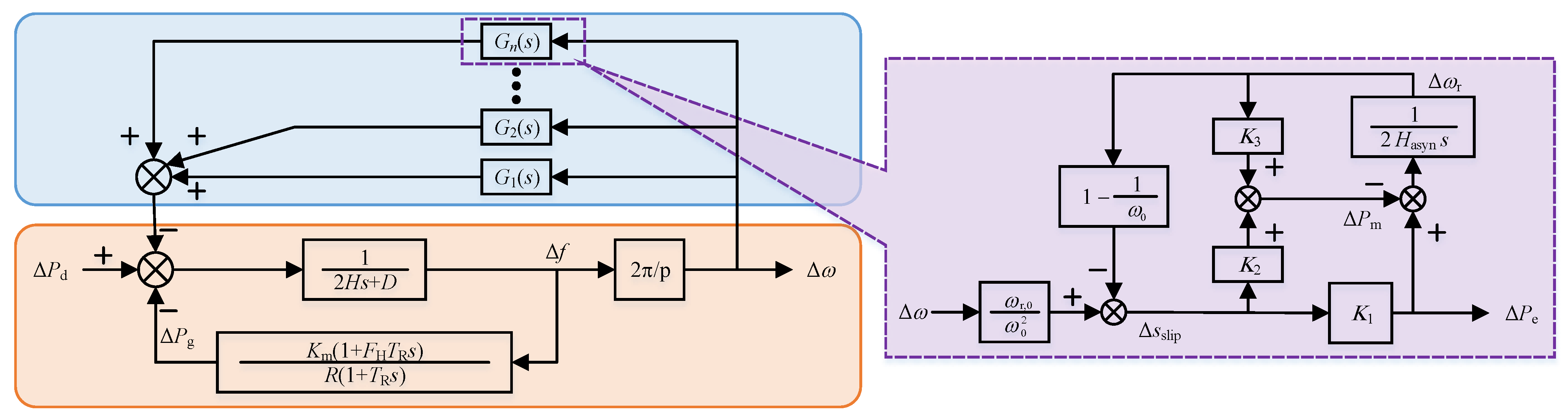
3.1. Dynamic Equivalent Model of the Grid Considering Multiple Induction Motors

With the detailed grid frequency response model, the grid frequency dynamics that consider multiple induction motors can be reproduced roughly, which will be further verified in Section 4.1. Nevertheless, from Figure 5, we can see that this detailed model is structurally complex and requires the specific parameters of induction motors. As a result, it remains a challenge to apply the detailed model in practice.
To fill this gap, a grid dynamic equivalent model (DEM) will be proposed in this section, as shown in Figure 6. From this figure, we can find the proposed DEM is the same structure as the low-order system frequency response model, but with different parameter values. Specifically, the grid damping coefficient and inertia constant are replaced by the corresponding equivalent values, that is, H and D are replaced by H e and D e , respectively. These two equivalent values can be identified using the data-driven approach, which will be introduced in the next section. The DEM is structurally simpler and therefore easier to apply in practice compared with the detailed grid frequency response model.
Once the dynamic equivalent model is derived, its parameters should be identified. To do so, firstly, the actual system, i.e., the modified IEEE 9-bus system, is established and evaluated. The actual IEEE 9-bus system will be present in Section 4. The evaluated results will be shown in Section 4.2. Secondly, m scenarios are simulated by adjusting the load disturbance Δ P d in the actual IEEE 9-bus system. In this work, m = 3 scenarios are simulated, where Δ P d is set to 1%, 3%, and 5%, respectively. In this manner, the dynamic behavior of the grid frequency can be observed, and the resulting frequency response curve can be sampled and labeled as Δ f ( i , j ) . Here, i 1 , 2 , . . . , m represents the i-th scenario and j 1 , 2 , . . . , n represents the j-th sample points in the i-th scenario. It should be observed that the sampling rate must not surpass 1 ms, taking into account the nominal frequency of the utility grid being 50 or 60 Hz. Any sampling rate exceeding 1 ms would result in sampling failure [24]. Thirdly, the same simulation scenarios are repeated using the dynamic equivalent model. Similarly, the corresponding frequency response curve is recorded and denoted by Δ f e ( i , j ) . Finally, with the aim of minimizing the mismatch between Δ f ( i , j ) and Δ f e ( i , j ) , H e and D e are identified by solving the optimal problem. In the following parts, special attention is paid to the detailed formulation and solution of the optimal problem.

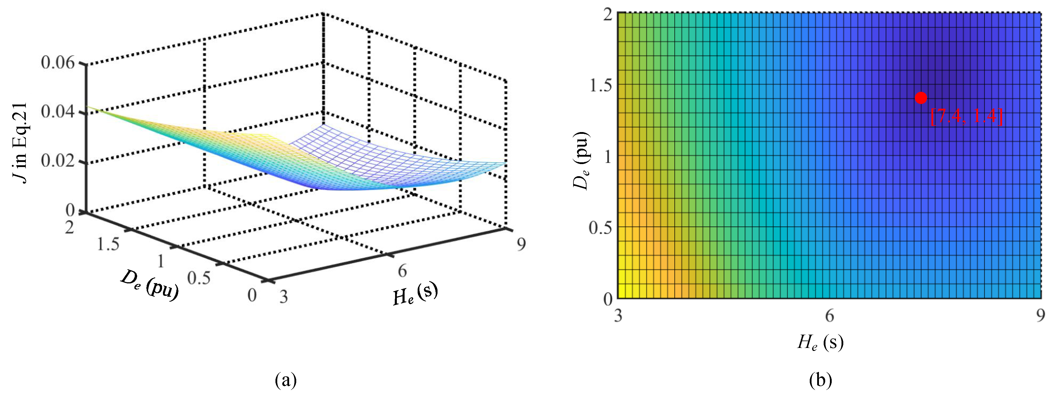
3.2. Formulation of the Optimal Problem

To identify the best fitting parameters H e and D e , an optimal problem should be developed. In general, there are two major elements for optimal problem formulation, i.e., objective function and constraints.
  • Objective Function
    As mentioned before, the aim of the identification approach is to minimize the mismatch between Δ f ( i , j ) and Δ f e ( i , j ) . In this point of view, the objective function is described as
    min J = i = 1 m j = 1 n Δ f ( i , j ) Δ f e ( i , j ) n
    Here, n denotes the sampling point numbers in one scenario and m denotes the simulated scenarios numbers.
  • Constraints
    The identified equivalent H e and D e should also be limited within a feasible range. In general, the grid inertia constant is 3~9 s and the grid damping coefficient is 0~2, which can be represented as [28]
    3 H e 9 0 D e 2

3.3. Solution of the Optimal Problem

From (19) and (20), we can see that Δ f ( i , j ) is the sampled data from the simulation of the actual system, and as a result, the optimal problem is without stringent mathematical formulation. Moreover, this optimal problem is highly non-convex. From these points of view, it is difficult to obtain the solution of the optimal problem (19) and (20) using the traditional gradient-based optimizing procedure. To address this issue, a genetic algorithm (GA) is introduced. GAs are known for their robustness and their ability to search adaptively for the global optimal point in a stochastic and discrete manner. They operate based on the mechanics of natural selection and genetics, enabling them to evolve an initial set of poor solution guesses into a set of acceptable solutions. In the following parts, special attention is paid to the steps using a GA for identification of H e and D e .
As for the optimal procedure for the GA, the parameters to be identified need to first be determined. In this paper, the damping coefficient D e and grid inertia constant H e are the two parameters to be identified. In other words, H e and D e need to be optimized so that the equivalent model can reproduce the actual grid frequency dynamics. Once the parameters to be identified are determined, a set of these parameters with specific values, i.e., vector H e , D e , constitutes an individual. Further, N p individuals generated randomly make up the initial population. To facilitate genetic manipulation, individuals are represented in binary form. That is, each individual is an N b -bit Gray encoding of a vector H e , D e .
After the population is generated, each individual, i.e., vector H e , D e , has a specific value. Considering the fact that the main objective of the identification approach is to minimize the mismatch between Δ f ( i , j ) and Δ f e ( i , j ) , for k-th individual, its fitness value can be calculated by
J k = i = 1 m j = 1 n Δ f k ( i , j ) Δ f e , k ( i , j ) n
Further, the average fitness value of the whole population can be represented as
F = l = 1 N p J k N p = i = 1 m j = 1 n l = 1 N p Δ f l ( i , j ) Δ f e , l ( i , j ) n N p
Here, N p is the number of individuals in the population. In this work, N p = 20 .
Genetic operations, that is, mutation, crossover, and selection, can be facilitated and the next population is generated, with fitness of individuals and population. Finally, the iteration will be stopped as soon as the termination criterion is met. Otherwise, the fitness of the population will be recalculated and using genetic operations, the new population will be generated. Please refer to Table 2 for more details about the genetic operations and termination criterion.
Remark 1.
In this work, considering the fact that the optimal problem (19) and (20) is high non-convexity, one of the intelligence algorithms, i.e., a genetic algorithm, has been employed to identify the equivalent parameters of the grid dynamic equivalent model. However, these intelligent algorithms may not guarantee the globally optimal values once the termination criterion has been achieved. In other words, the solution calculated by the intelligent algorithm may be a locally optimal one. Even worse, in the presence of an optimal problem with multiple local minima, the assurance of achieving a globally optimal solution cannot be guaranteed upon subsequent execution of the intelligent algorithm. Fortunately, an ad hoc approach makes it possible to fill this gap. By plotting the J, i.e., (21), in terms of H e and D e , this ad hoc approach can provide the globally optimal value. Nevertheless, there remains a concern with employing the ad hoc approach. That is, the accuracy and computational cost of the method are determined by the mesh partition of H e and D e . Specifically, if the partition step size is too large, the calculation results may not meet the required level of accuracy and the computational cost may become prohibitively high. From the above observations, we employ the genetic algorithm to find the optimal solution of the problem (19) and (20). Meanwhile, the ad hoc approach with a slightly larger partition step size is employed to guarantee the solution of the genetic algorithm is the globally optimal one.
Table 2. Steps of the GA-based identification approach.
StepDescription
Step 1Initialize the population: In the initialization phase, N p individuals are created to form the initial population. Each individual is an N b -bit Gray encoding of a vector H e , D e . In other words, each individual denotes a feasible solution to the optimal problem (19) and (20).
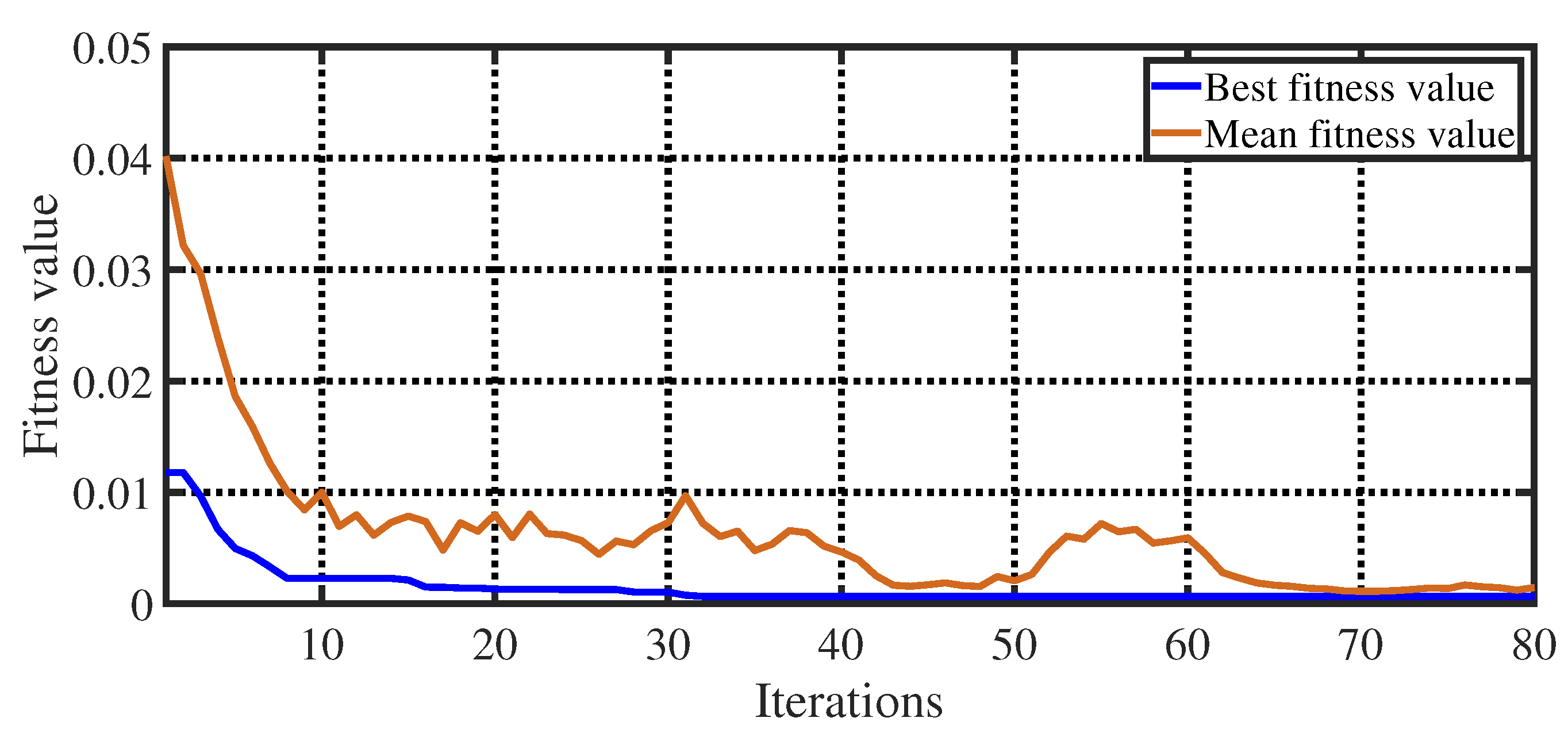
Step 2Calculate fitness value: The main objective of the data-driven-based identification approach is to minimize the mismatch between Δ f ( i , j ) and Δ f e ( i , j ) . As a result, for k-th individual, its fitness value can be calculated by J k = i = 1 m j = 1 n Δ f k ( i , j ) Δ f e , k ( i , j ) Δ f k ( i , j ) Δ f e , k ( i , j ) n n . Correspondingly, the average fitness value of the whole population can be represented as F = k = 1 N p J k J k N p N p = i = 1 m j = 1 n k = 1 N p Δ f k ( i , j ) Δ f e , k ( i , j ) Δ f k ( i , j ) Δ f e , k ( i , j ) ( n N p ) ( n N p ) .
Step 3Generate the new population by selection, crossover, and mutation.
  • Selection: Some of the individuals in the current population have lower fitness value, which means that they may the optimal solutions. As a result, these individuals are directly selected in the next population. In this work, 5% of individuals are directly selected in the next population.
  • Crossover: Besides the selection, two of the individuals are randomly selected and some part of their binary coding is exchanged to form the new individuals. In this work, the crossover fraction is 0.8.
  • Mutation: For the newly generated population, some of the individuals are selected in a random way. Further, some part of these selected individuals’ binary coding is changed. In this work, the mutation fraction is 0.2.
  • Individuals that do not meet the constraints (20) are removed from the population.
Step 4Termination criterion: The iteration is stopped as soon as any one of these two condition is met. Otherwise, the algorithm goes back to Step 2.
  • The quantity of generations: The algorithm will stop when the number of generations reaches its threshold setting, i.e., 100.
  • The change of fitness value: The algorithm will stop when the average relative change in the fitness value is less than its threshold setting, i.e., 0.001.

3.4. Performance Evaluation of the Grid Model Considering Multiple Induction Motors

Up to now, considering multiple induction motors, the dynamic equivalent model and detailed grid frequency model have been proposed. Before discussing the influence of induction motors on grid frequency with the proposed models, their performance needs to be evaluated. In other words, the accuracy of the proposed models should be analyzed. To do so, the following two error indicators are introduced.
I E ( t ) = f ( t ) f a ( t ) f a ( t ) f n
A E ( t ) = 0 t f ( t ) f a ( t ) d t 0 t f a ( t ) f n d t
Here, I E ( t ) denotes the instantaneous error at t, A E ( t ) denotes the accumulative error at t, f a ( t ) is the frequency curve of the real grid, f ( t ) is the frequency curve of the proposed model during a frequency event, and f n is the normal frequency of the grid, i.e., 50 Hz in this work.
From the definitions of the two error indicators, we can see that I E ( t ) and A E ( t ) indicate the accuracy of the proposed models. The larger the I E ( t ) and A E ( t ) , the less accurate the proposed models. That is, larger I E ( t ) and A E ( t ) indicate larger mismatch between the frequency model and the actual grid.
Remark 2.
It is noted that the above two error indicators are a posteriori ones. That is, these two indicators can be calculated only after the frequency response curves of the actual system and the model are recorded. In other words, these two indicators cannot be used for the traditional model alone, which are not satisfactory. This will be our future research focus.

4. Simulation Studies

The present section assesses the performance of the detailed grid frequency response model proposed in Section 2.3 and the dynamic equivalent model proposed in Section 3.1. To accomplish this, five cases are conducted, which are outlined as follows:
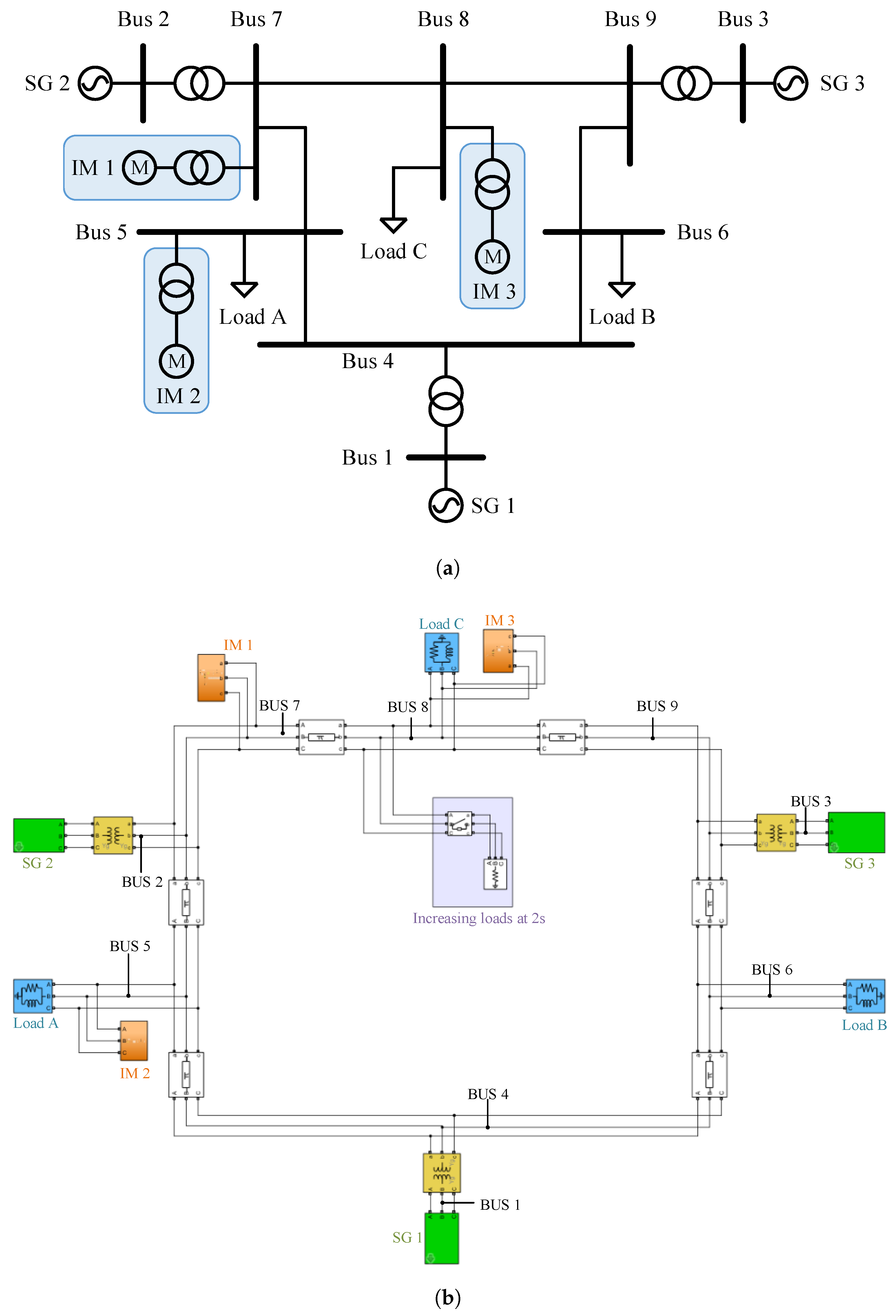
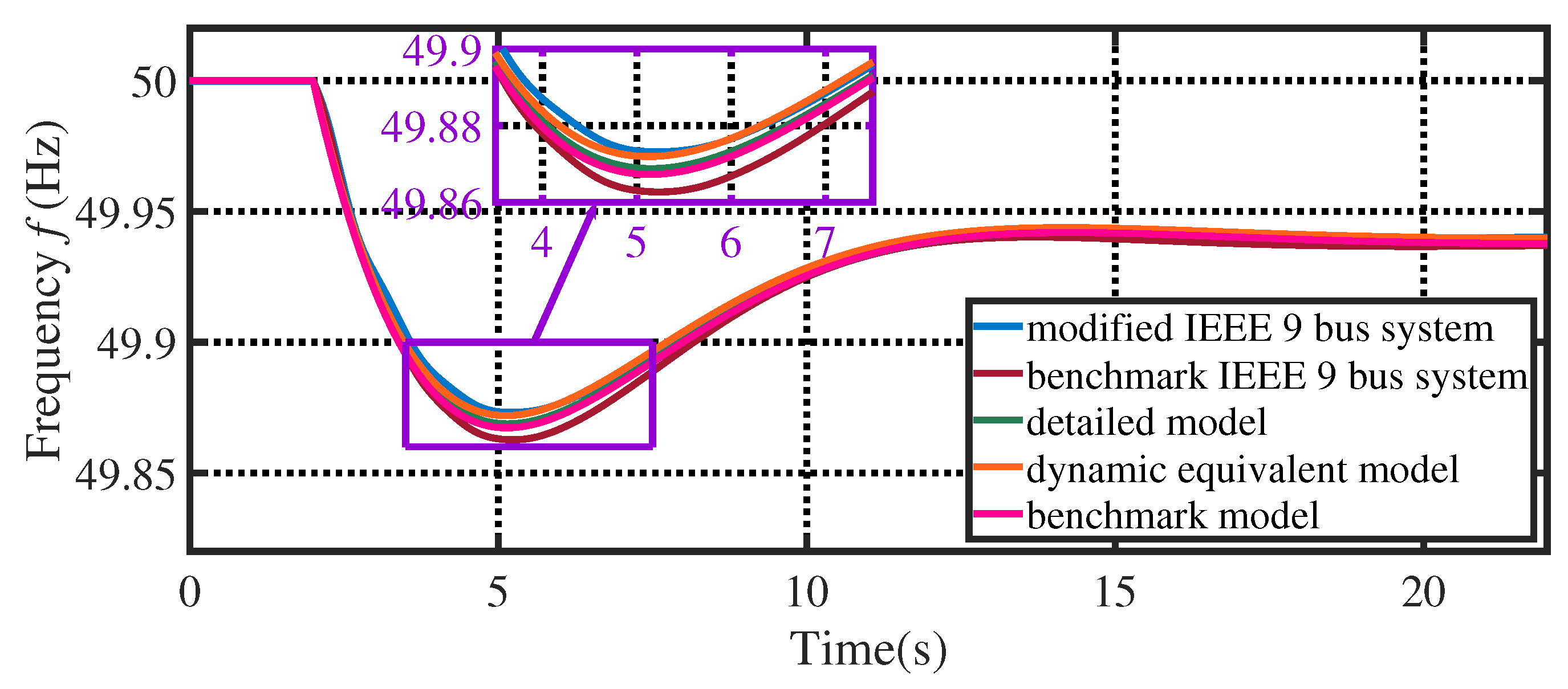
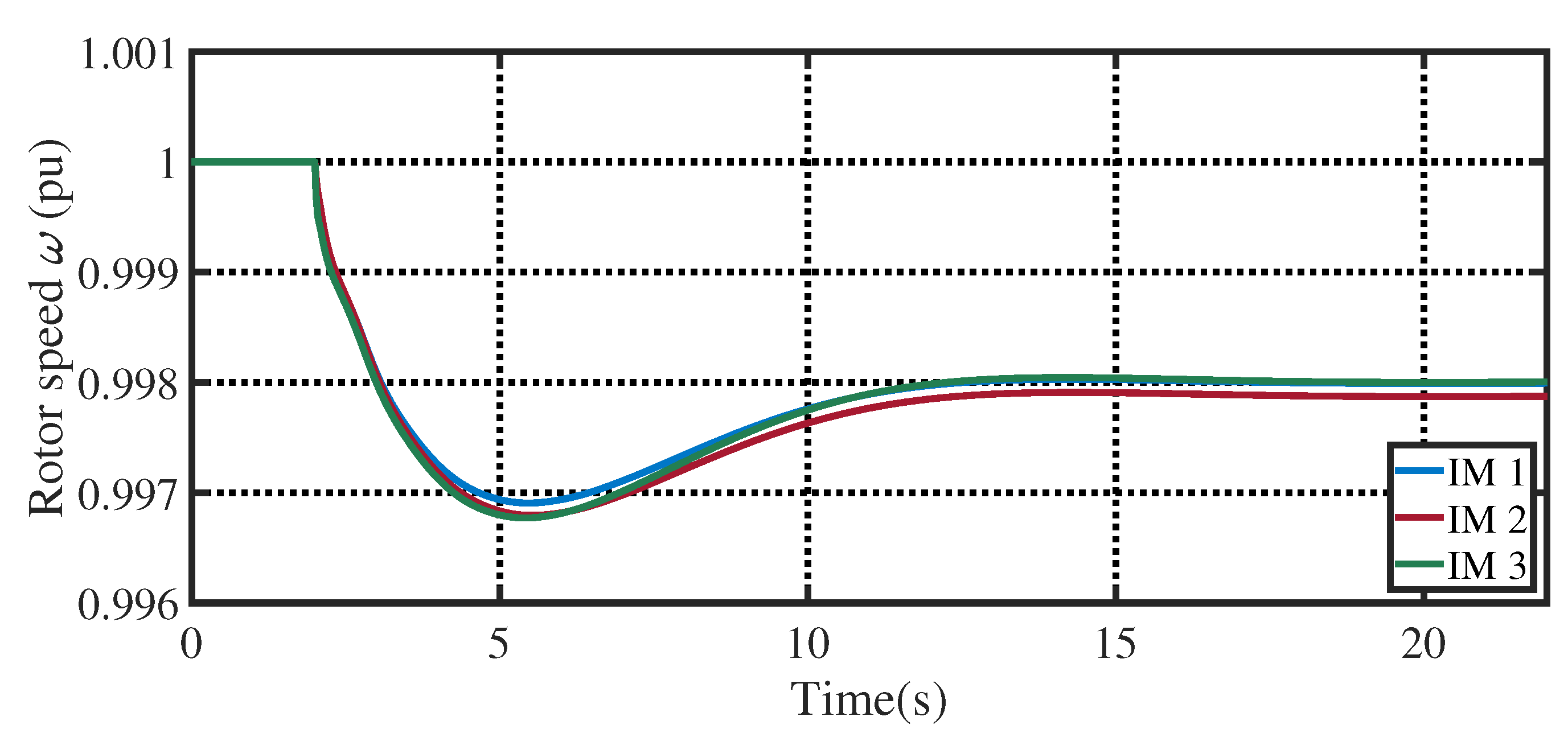
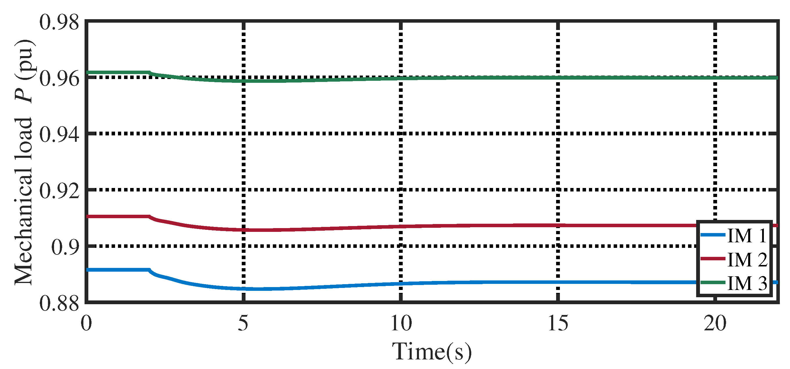
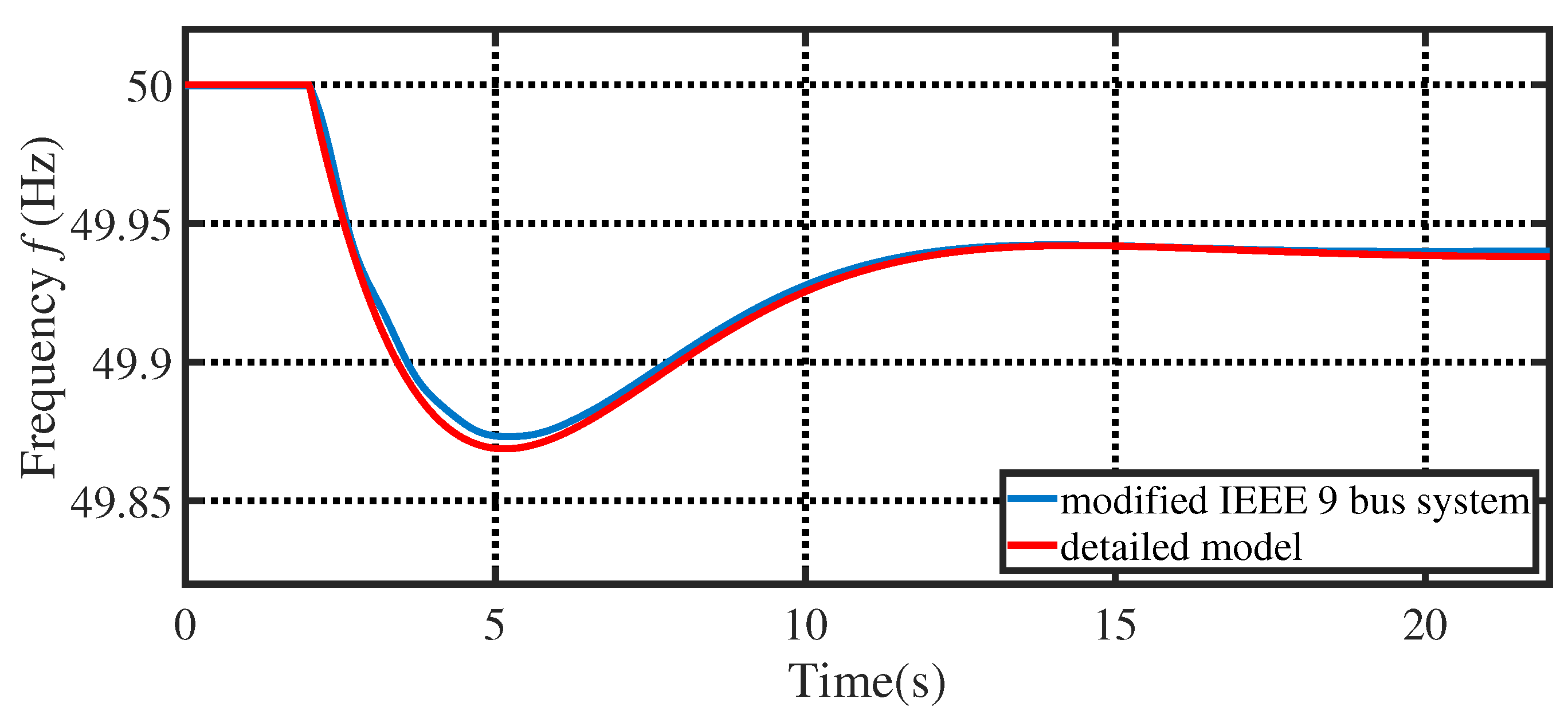
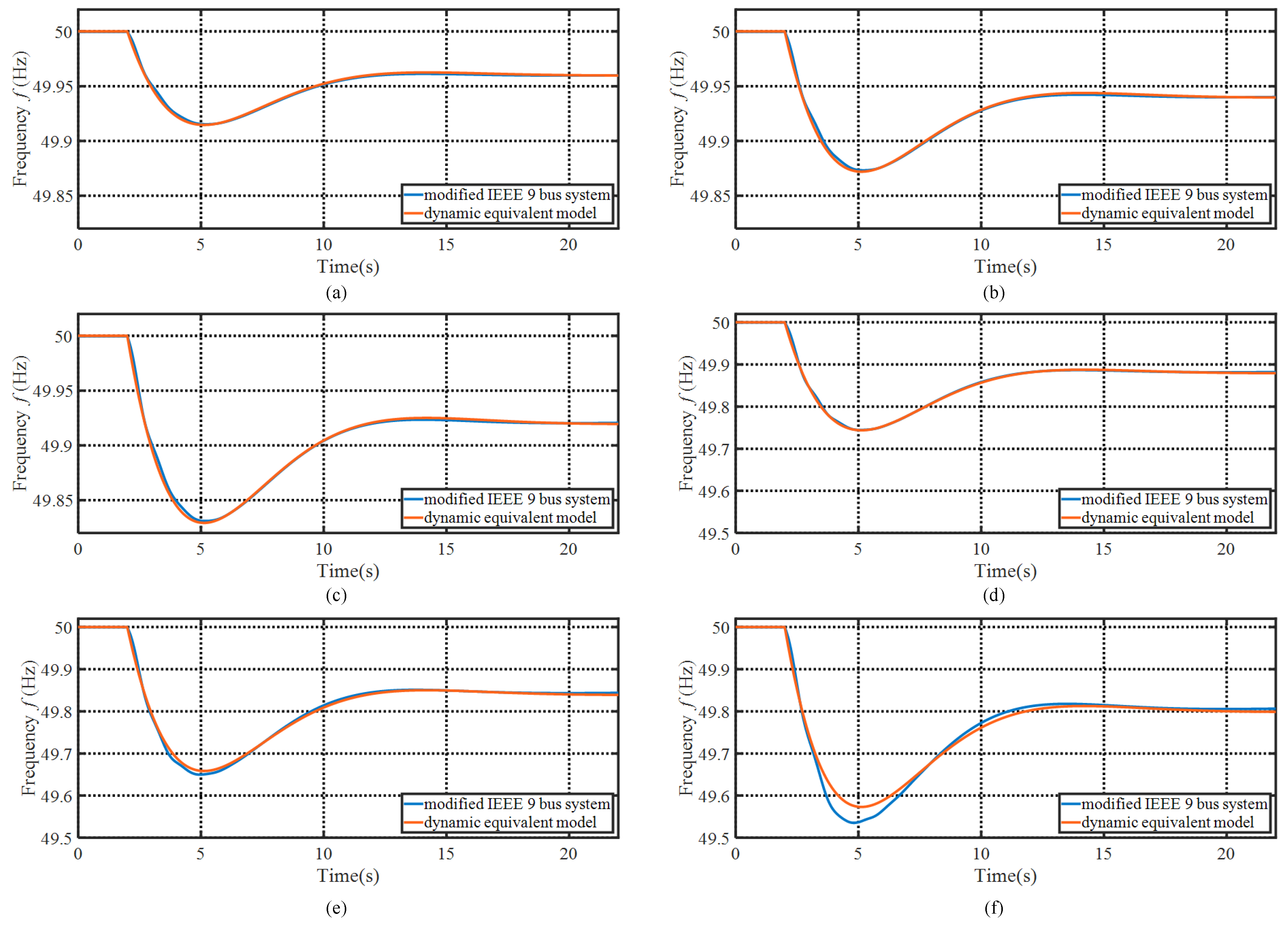
  • Modified IEEE 9-bus system: The modified IEEE 9-bus system is implemented in MATLAB Simulink using the Special Power Systems library, whose block diagram is shown in Figure 7. It is the modified version of the actual IEEE 9-bus system. In the modified system, there are three synchronous generators, that is, SG 1, SG 2, and SG 3, on the generation-side. All of them are connected to the grid via transformers. The parameters of these three synchronous generators are presented in Table A1. On the consumption-side, three constant loads, i.e., Load A, Load B, and Load C, are connected to the grid, and whose parameters are listed in Table A2. Moreover, three induction motors, that is, IM 1, IM 2, and IM 3, are also integrated into the grid on Bus 7, Bus 5, and Bus 8, respectively. Considering that the induction motors are predominantly employed in high energy consumption enterprises, where they are either in operation or planned to be stopped, the operation conditions of these three induction motors are assumed unchanged, that is, they always work near the initial operation point. The parameters of the induction motors, transformers, and transmission lines are shown in Table A3, Table A4 and Table A5, respectively.
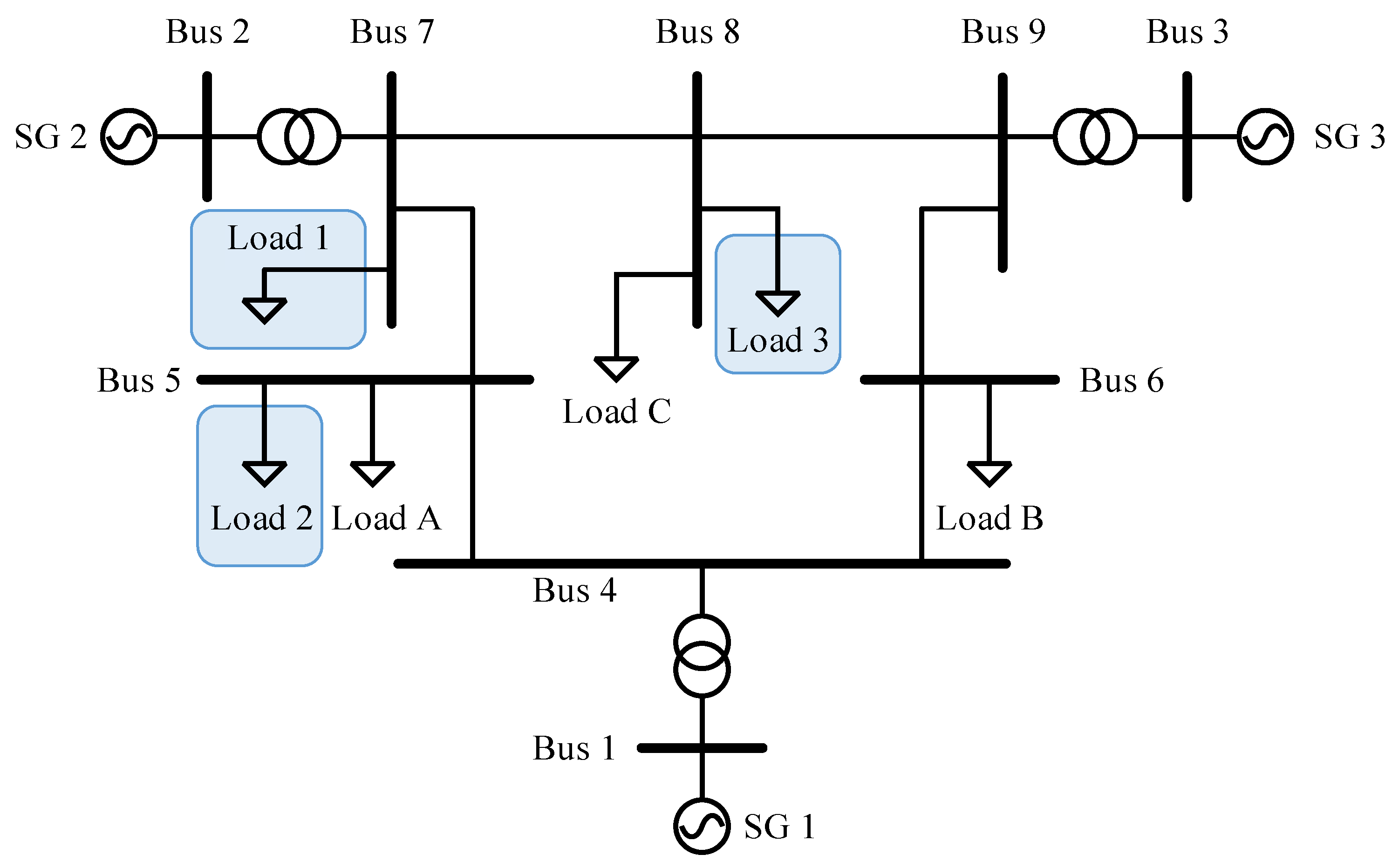
  • Benchmark IEEE 9-bus system: The benchmark IEEE 9-bus system is derived from the above modified IEEE 9-bus system, whose block diagram is shown in Figure 8. The benchmark IEEE 9-bus system is also implemented in MATLAB Simulink using the Special Power Systems library. The only difference between these two systems is that in the benchmark system, the induction motors are replaced with the equal capacity constant loads. Specifically, IM 1, IM 2, and IM3 are replaced with Load 1, Load 2, and Load 3, respectively, whose parameters are listed in Table A6.
  • Detailed model: The detailed model is proposed in Section 2.3, whose block diagram is shown in Figure 5. This model is also implemented in the MATLAB Simulink platform.
  • Dynamic equivalent model: The dynamic equivalent model is proposed in Section 3.1, whose block diagram is shown in Figure 6. This model and its identification approach are implemented using MATLAB scripts.
  • Benchmark model: The benchmark model is proposed in [21]. In this model, only an aggregated induction model is used to emulate the influence of induction motors on the grid frequency dynamics.

4.1. Influence of the Induction Motors on Grid Frequency Dynamics

As mentioned in introduction, there are a considerable amount of induction motors in a grid, which would contribute to grid inertia due to their stored kinetic energy and mechanical loads. In this subsection, the influence of the induction motors on the grid frequency dynamics will be presented. To do so, the frequency dynamics of different cases are studied during the under-frequency events. To cause an under-frequency event, in the modified and benchmark IEEE 9-bus system, a step increase of 10% active power of Load C (i.e., 3% of total load) is simulated at 2.0 s. Correspondingly, in the detailed model, dynamic equivalent model, and benchmark model, a step increase of 3% of total load is also simulated at 2.0 s. The result for this case is shown in Figure 9.
Figure 9 presents the grid frequency dynamics of different cases during the under-frequency event. From this figure, we can see that during the early stage of the frequency event (i.e., 2.0~2.8 s), the frequency dynamics of the modified IEEE 9-bus system is nearly same as that of the benchmark IEEE 9-bus system. After that, the frequency of the modified IEEE 9-bus system is always above that of the benchmark IEEE 9-bus system. Specifically, the frequency nadir of the modified IEEE 9-bus system is 49.87 Hz (appears at t = 5.1 s), which is higher than that of the benchmark IEEE 9-bus system, i.e., 49.86 Hz (appears at t = 5.2 s). At the steady-state stage, the frequency of the modified IEEE 9-bus system is steady at 49.94 Hz, while that of the benchmark IEEE 9-bus system also constant at 49.94 Hz. The above simulation results indicate that in addition to the synchronous units on generation-side, the induction motors on consumption-side also have a great influence on the grid frequency dynamics. The reason is because of the fact that when the grid frequency decreases (or increases), the rotor speed of the induction motors decelerate (or accelerate). Correspondingly, the kinetic energy stored in the rotating rotor is naturally used to provide frequency support. Moreover, when the grid frequency decreases (or increases), the mechanical loads of the inductions will change, and thus need less (or more) active power from the grid.
It is noted that from Figure 9, we can also see that in comparing the benchmark model and detailed model, the the fidelity of the dynamic equivalent model is higher. This will be further verified in Section 4.2 and Section 4.3.
Figure 10 presents the induction motors’ rotor speed dynamics in the modified IEEE 9-bus system during the under-frequency event. From this figure, we can see that after the under-frequency event, the active power absorbed by the induction motors decreases. The reason being that when the grid frequency decreases, the rotor speed of the induction motors decelerates, as shown in Figure 10. Correspondingly, the kinetic energy stored in the rotating rotor is naturally released to provide frequency support.
Moreover, in Figure 11, the induction motors’ mechanical load dynamics in the modified IEEE 9-bus system during the under-frequency event is also presented. From this figure, we can see that after the under-frequency event, the mechanical loads of the inductions have changed. Specifically, when the grid frequency decreases (or increases), the mechanical loads of the inductions correspondingly decreases (or increases), and thus need less (or more) active power from the grid.
Form Figure 10 and Figure 11, we can see that the consumption-side induction motors in grid do effect the grid frequency dynamics with their kinetic energy and mechanical loads. Moreover, this effect depends on the parameters and working conditions of the induction motors. In this work, the parameters and working conditions of the induction motors have been listed in Table A3, where we can see that the parameters and working conditions of the induction motors are all different from each other. This causes the difference in the values of the rotor speed and mechanical load of the induction motors during the under-frequency event.

4.2. Accuracy of the Detailed Grid Frequency Response Model Considering Multiple Induction Motors

In this subsection, the accuracy of the detailed grid frequency response model considering multiple induction motors, i.e., detailed model, is evaluated.
To do so, the frequency dynamics of the modified IEEE 9-bus system and that of the detailed model are simulated and plotted, as shown in Figure 12. From this figure, we can see that the proposed detailed model can reproduce the grid frequency dynamics of the modified IEEE 9-bus system with a high degree of fidelity. Specifically, during the early stage of the frequency event (i.e., 2.0~2.8 s), the frequency dynamics of the detailed model are nearly same as those of the modified IEEE 9-bus system. In the frequency recovery phase (i.e., 5.1~12 s), the frequency of the detailed model is slightly higher than that of the modified IEEE 9-bus system. At the steady-state stage (i.e., 18.0~22.0 s), the frequency of the detailed model becomes slightly lower than that of the modified IEEE 9-bus system.
To further verify the accuracy of the detailed grid frequency response model, its instantaneous error and accumulative error are calculated and shown in Figure 13. To obtain the instantaneous error and accumulative error, the frequency curve of the detailed model is selected as f ( t ) in (23) and (24), meanwhile, the frequency curve of the modified IEEE 9-bus system is selected as f n ( t ) . From Figure 13, we can find that both the maximum instantaneous error and maximum accumulative error are less than 10%, which appears at t = 2.3 s. From these points of view, it is shown that the proposed detailed grid frequency response model is a fair fidelity model.

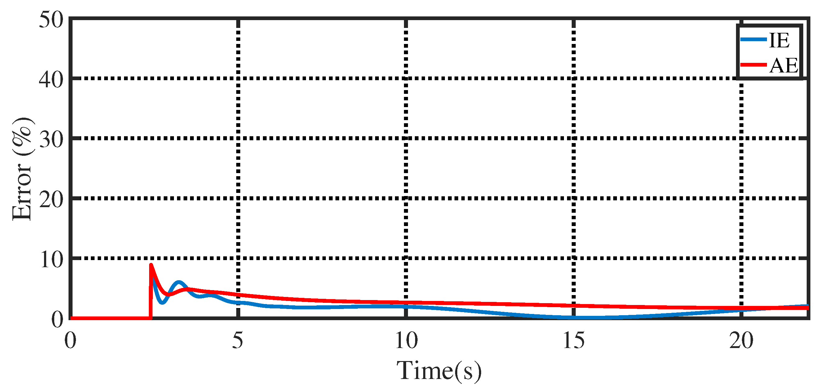
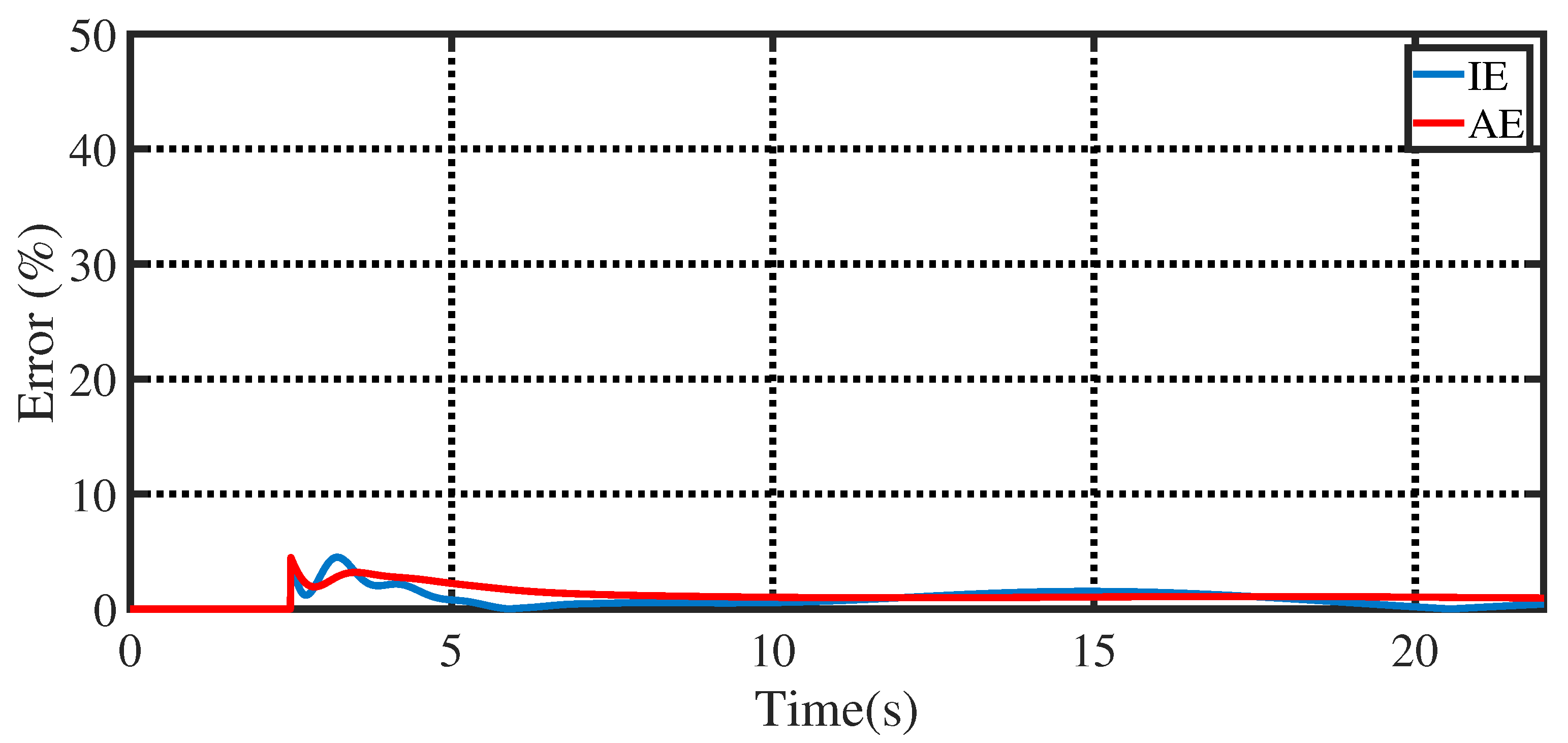
4.3. Dynamic Equivalent Model Identification and Its Accuracy

Although the detailed model can reproduce the frequency dynamics of the grid with multiple induction motors, it is structurally complex and requires the specific parameters of induction motors. To fill this gap, the dynamic equivalent model is derived in Section 3.1, and its equivalent parameters can be identified using the data-driven approach proposed in Section 3.2 and Section 3.3. In this subsection, the parameters’ identification results and the accuracy of the proposed dynamic equivalent model are going to be presented.
Table 3 presents the inertia constant (H) and frequency damping coefficient (D) of the detailed model. These two parameters are derived from the benchmark IEEE 9-bus system. That is, H and D represent the original inertia constant and frequency damping coefficient of the modified IEEE 9-bus system without considering multiple induction motors. Moreover, the identified equivalent inertia constant ( H e ) and frequency damping coefficient ( D e ) are also listed in Table 3, where we can see that not only does the inertia constant increase, but the frequency damping coefficient also increases after considering the multiple induction motors in grid.
The fitness value dynamics during the identification process are plotted in Figure 14. From this figure, the conclusion can be drawn that after 80 iterations, the fitness of the optimal individual and the mean fitness of the population tend to be stable. This indicates that the equivalent inertia constant ( H e ) and frequency damping coefficient ( D e ) are the optimal solutions.
As mentioned in Section 3.3, intelligent algorithms may not guarantee the globally optimal values once the termination criterion has been achieved. In other words, the solution calculated by the intelligent algorithm may be a locally optimal one. To fill this gap, the ad hoc approach is introduced. By plotting the J in terms of H e and D e , this ad hoc approach can roughly provide the globally optimal value. To do so, partition step size of H e and D e is set to 0.1, that is, J is plotted in terms of 61 H e (i.e., 3.0, 3.1, …, 9.0) and 21 D e (i.e., 0.0 0.1, …, 2.0). The results are shown in Figure 15. The computational cost of the GA-based identification method and ad hoc method are listed in Table 4.
From Figure 15 and Table 4, we can see that the identification results of the ad hoc method (i.e., H e = 7.4 , D e = 1.4 ) are nearly the same as those of the GA-based identification method (i.e., H e = 7.4230 , D e = 1.4070 ). In Figure 15, darker and cooler colors represent better fit results. From this point of view, the identification results calculated by GA are the globally optimal ones. Moreover, compared with the ad hoc method, the GA-based identification method is more accurate, that is, its solutions can achieve accuracy up to four decimal places. Although the ad hoc method can achieve the same accuracy by reducing the partition step size of H e and D e , it is computationally expensive to do so.
Once the optimal equivalent inertia constant ( H e ) and frequency damping coefficient ( D e ) are identified, the grid dynamics can be studied using the dynamic equivalent model. Figure 16 shows the grid frequency dynamics of the modified IEEE 9-bus system, the detailed model, and the dynamic equivalent model during the under-frequency event. As seen from this figure, the proposed dynamic equivalent model can reproduce the grid frequency dynamics of the modified IEEE 9-bus system with a higher degree of fidelity than the detailed model, which benefits from the selection of multiple scenarios when identifying H e and D e .
Figure 17 further verifies the the accuracy of the dynamic equivalent model. In this figure, the instantaneous error and accumulative error of the dynamic equivalent model are calculated and presented. To obtain the instantaneous error and accumulative error, the frequency curve of the dynamic equivalent model is selected as f ( t ) in (23) and (24), meanwhile, the frequency curve of the modified IEEE 9-bus system is selected as f n ( t ) . From Figure 17, we can find that both the maximum instantaneous error and the accumulative error are less than 5%. From this point of view, the fidelity of the proposed dynamic equivalent model is higher than the detailed grid frequency response model.

4.4. Influence of the Grid Load Disturbance on the Dynamic Equivalent Model Accuracy

In Section 3, three scenarios, where the grid load disturbance Δ P d is set to 1%, 3%, and 5%, are employed to identify the parameters of the dynamic equivalent model. In this section, the influence of the grid load disturbance on the dynamic equivalent model accuracy is going to be investigated.
To do so, five additional scenarios, where the grid load disturbance Δ P d is set to 2%, 4%, 6%, 8%, and 10%, are employed. The frequency dynamics of the IEEE 9-bus system and dynamic equivalent model under different load disturbance Δ P d have been presented in Figure 18. From this figure, we can see that when | Δ P d | < 8 % , the dynamic equivalent model can accurately reproduce the frequency dynamics of a grid with multiple induction motors. However, when the grid load disturbance is too large (such as | Δ P d | = 10 % ), the fidelity of the model is reduced. From this point of view, the proposed dynamic equivalent model is more accurate in the case of small grid load disturbance.

5. Conclusions

In this paper, the influence of induction motors on grid inertia are investigated. To do so, in this paper, we propose two types of models, i.e., the detailed grid model and dynamic equivalent model considering multiple induction motors. Specifically, a detailed grid model with multiple induction motors is first established. However, the detailed model requires the specific parameters of induction motors, which are hard to acquire in large systems. Moreover, the accuracy of the model is unsatisfactory. To fill these gaps, a dynamic equivalent model (DEM) is further proposed to emulate the detailed model. Compared with the detailed model, the proposed dynamic equivalent model is structurally simple and does not require the specific parameters of induction motors. Therefore, it is possible to apply it to large systems to investigate the influence of induction motors on grid frequency dynamics. To figure out the parameters of the proposed dynamic equivalent model from historical frequency data, a genetic algorithm approach is introduced. The proposed models are evaluated on the IEEE 9-bus system in MATLAB and SimPowerSystems toolbox, which verifies their accuracy and effectiveness.
The key contributions of the paper are threefold.
  • A detailed grid model incorporating multiple induction motors is established to imitate the influence of induction motors on grid inertia.
  • To address the limitations of the detailed grid model, a dynamic equivalent model is further proposed. Compared with the detailed model, the proposed dynamic equivalent model is structurally simple and does not require the specific parameters of induction motors. So it is possible to be applied to large systems.
  • A genetic algorithm-based approach is introduced to identify the parameters of the dynamic equivalent model. Its optimality is guaranteed by an ad hoc approach.
In this work, all of the induction motors are assumed to work near the initial operation point. Considering the random characteristics of induction motors, it is crucial to investigate the effects of random motor start-up and shutdown events, which will be our future research focus.

Author Contributions

Conceptualization, Z.T., G.M. and P.K.; methodology, Z.T., G.M., H.Y., J.P., P.K., M.M. and Z.Z.; software, Z.T., H.Y., M.M. and Z.Z.; validation, G.M., H.Y. and Z.X.; investigation, Z.T., G.M. and P.K.; resources, H.Y., J.P. and Z.X.; writing—original draft preparation, Z.Z.; writing—review and editing, Z.T., P.K. and M.M.; visualization, H.Y.; supervision, Z.T. and G.M.; project administration, P.K.; funding acquisition, Z.T. All authors have read and agreed to the published version of the manuscript.

Funding

This research was funded by the Science and Technology Project of State Grid Shanxi Electric Power Research Institute.(Project name: Research on equivalent inertia and frequency response characteristics of induction motors and applications of black-start scheme in power grid, Project number: 52053022000J).

Data Availability Statement

Not applicable.

Conflicts of Interest

The authors declare no conflict of interest.

Appendix A

Table A1. The parameters of the synchronous generators.
ParametersSG 1SG 2SG 3
Rated power S n (MVA)250220128
Line-to-line voltage V (kV)16.51813.8
Rated frequency f n (Hz)505050
Inertia coefficient H (s)666
Stator resistance R s (pu)0.0040.0040.004
d axis reactance X d , X d , X d (pu)1.7, 0.27, 0.21.7, 0.27, 0.21.7, 0.27, 0.2
q axis reactance X q , X q , X q (pu)1.65, 0.47, 0.21.65, 0.47, 0.21.65, 0.47, 0.2
Table A2. The parameters of the constant loads, i.e., Load A, Load B, and Load C.
ParametersLoad ALoad BLoad C
Rated active power P n (MW)12590100
Rated reactive power Q n (MVar)503035
Table A3. The parameters of the induction motors.
ParametersIM 1IM 2IM 3
Rated power S n (MVA)353218
Rated frequency f n (Hz)505050
Stator resistance and inductance R s , L s (pu)0.020, 0.0400.014, 0.0350.022, 0.043
Rotor resistance and inductance R r , L r (pu)0.019, 0.0400.017, 0.0360.021, 0.042
Mechanical loads (pu) T m = 0.5 ω r + 0.5 ω r 2 T m = 0.5 + 0.3 ω r + 0.2 ω r 2 T m = 1
Mechanical loads typeconstant-power load and pump loadconstant-torque load, constant-power load and pump loadconstant-torque load
Table A4. The parameters of the transformers.
LocationNominal Power (MVA)Nominal Frequency (Hz)Winding 1 Parameters [R1(pu), L1(pu)]Winding 2 Parameters [R2(pu), L2(pu)]
Bus 1–Bus 425050[0, 0.15][0, 0.15]
Bus 2–Bus 722050[0.15, 0][0.15, 0.05]
Bus 3–Bus 915050[0, 0][0, 0.15]
Table A5. The parameters of the transmission lines.
LocationLengthResistances (Ohms/km)Inductances (mH/km)Capacitances (uF/km)
Bus 4–Bus 516.7554.70.31
Bus 4–Bus 616.7554.70.31
Bus 5–Bus 716.7554.70.31
Bus 6–Bus 916.7554.70.31
Bus 7–Bus 816.7554.70.31
Bus 8–Bus 916.7554.70.31
Table A6. The parameters of the constant loads, i.e., Load 1, Load 2, and Load 3.
ParametersLoad 1Load 2Load 3
Rated active power P n (MW)353218

References

  1. Qi, J.; Liu, L.; Shen, Z.; Xu, B.; Leung, K.S.; Sun, Y. Low-carbon community adaptive energy management optimization toward smart services. IEEE Trans. Ind. Inform. 2019, 16, 3587–3596. [Google Scholar] [CrossRef]
  2. Alotaibi, I.; Abido, M.A.; Khalid, M.; Savkin, A.V. A comprehensive review of recent advances in smart grids: A sustainable future with renewable energy resources. Energies 2020, 13, 6269. [Google Scholar] [CrossRef]
  3. Kalantar-Neyestanaki, M.; Cherkaoui, R. Coordinating distributed energy resources and utility-scale battery energy storage system for power flexibility provision under uncertainty. IEEE Trans. Sustain. Energy 2021, 12, 1853–1863. [Google Scholar] [CrossRef]
  4. Muttaqi, K.M.; Islam, M.R.; Sutanto, D. Future power distribution grids: Integration of renewable energy, energy storage, electric vehicles, superconductor, and magnetic bus. IEEE Trans. Appl. Supercond. 2019, 29, 1–5. [Google Scholar] [CrossRef]
  5. Zuo, K.; Wu, L. Enhanced Power and Energy Coordination for Batteries Under the Real-Time Closed-Loop, Distributed Microgrid Control. IEEE Trans. Sustain. Energy 2022, 13, 2027–2040. [Google Scholar] [CrossRef]
  6. Muttaqi, K.M.; Sutanto, D. Adaptive and predictive energy management strategy for real-time optimal power dispatch from vpps integrated with renewable energy and energy storage. IEEE Trans. Ind. Appl. 2021, 57, 1958–1972. [Google Scholar]
  7. Global Wind Energy Council. GWEC Global Wind Report 2022; Global Wind Energy Council: Brussels, Belgium, 2022. [Google Scholar]
  8. Xiao, Y.; Wang, X.; Wang, X. A modified intra-day market to trade updated forecast information for wind power integration. IEEE Trans. Sustain. Energy 2020, 12, 1044–1059. [Google Scholar] [CrossRef]
  9. Worku, M.Y.; Hassan, M.A.; Abido, M.A. Real time energy management and control of renewable energy based microgrid in grid connected and island modes. Energies 2019, 12, 276. [Google Scholar] [CrossRef]
  10. Fjellstedt, C.; Ullah, M.I.; Forslund, J.; Jonasson, E.; Temiz, I.; Thomas, K. A Review of AC and DC Collection Grids for Offshore Renewable Energy with a Qualitative Evaluation for Marine Energy Resources. Energies 2022, 15, 5816. [Google Scholar] [CrossRef]
  11. Lunardi, A.; Normandia Lourenço, L.F.; Munkhchuluun, E.; Meegahapola, L.; Sguarezi Filho, A.J. Grid-Connected Power Converters: An Overview of Control Strategies for Renewable Energy. Energies 2022, 15, 4151. [Google Scholar] [CrossRef]
  12. Xue, S.M.; Liu, C. Line-to-line fault analysis and location in a VSC-based low-voltage DC distribution network. Energies 2018, 11, 536. [Google Scholar] [CrossRef]
  13. Hu, Q.; Han, R.; Quan, X.; Wu, Z.; Tang, C.; Li, W.; Wang, W. Grid-forming inverter enabled virtual power plants with inertia support capability. IEEE Trans. Smart Grid 2022, 13, 4134–4143. [Google Scholar] [CrossRef]
  14. Li, C.; Yang, Y.; Cao, Y.; Aleshina, A.; Xu, J.; Blaabjerg, F. Grid inertia and damping support enabled by proposed virtual inductance control for grid-forming virtual synchronous generator. IEEE Trans. Power Electron. 2022, 38, 294–303. [Google Scholar] [CrossRef]
  15. Sockeel, N.; Gafford, J.; Papari, B.; Mazzola, M. Virtual inertia emulator-based model predictive control for grid frequency regulation considering high penetration of inverter-based energy storage system. IEEE Trans. Sustain. Energy 2020, 11, 2932–2939. [Google Scholar] [CrossRef]
  16. Qi, Y.; Deng, H.; Liu, X.; Tang, Y. Synthetic inertia control of grid-connected inverter considering the synchronization dynamics. IEEE Trans. Power Electron. 2021, 37, 1411–1421. [Google Scholar] [CrossRef]
  17. Björk, J.; Johansson, K.H.; Dörfler, F. Dynamic virtual power plant design for fast frequency reserves: Coordinating hydro and wind. IEEE Trans. Control. Netw. Syst. 2022. [Google Scholar] [CrossRef]
  18. Basak, R.; Bhuvaneswari, G.; Pillai, R.R. Low-voltage ride-through of a synchronous generator-based variable speed grid-interfaced wind energy conversion system. IEEE Trans. Ind. Appl. 2019, 56, 752–762. [Google Scholar] [CrossRef]
  19. Kabsha, M.; Rather, Z.H. A new control scheme for fast frequency support from HVDC connected offshore wind farm in low-inertia system. IEEE Trans. Sustain. Energy 2019, 11, 1829–1837. [Google Scholar] [CrossRef]
  20. Manaz, M.M.; Lu, C.N. Design of resonance damper for wind energy conversion system providing frequency support service to low inertia power systems. IEEE Trans. Power Syst. 2020, 35, 4297–4306. [Google Scholar] [CrossRef]
  21. Zhou, T.; Liu, Z.; Ye, H.; Ren, B.; Xu, Y.; Liu, Y. Frequency response modeling and equivalent inertial estimation of induction machine. Energy Rep. 2022, 8, 554–564. [Google Scholar] [CrossRef]
  22. Chen, L.; Wang, X.; Min, Y.; Li, G.; Wang, L.; Qi, J.; Xu, F. Modelling and investigating the impact of asynchronous inertia of induction motor on power system frequency response. Int. J. Electr. Power Energy Syst. 2020, 117, 105708. [Google Scholar] [CrossRef]
  23. Wang, D.; Yuan, X.; Zhang, M. Power-balancing based induction machine model for power system dynamic analysis in electromechanical timescale. Energies 2018, 11, 438. [Google Scholar] [CrossRef]
  24. Hu, Y.L.; Wu, Y.K. Inertial Response Identification Algorithm for the Development of Dynamic Equivalent Model of DFIG-Based Wind Power Plant. IEEE Trans. Ind. Appl. 2021, 57, 2104–2113. [Google Scholar] [CrossRef]
  25. Liu, Y.; Zhang, N.; Wang, Y.; Yang, J.; Kang, C. Data-driven power flow linearization: A regression approach. IEEE Trans. Smart Grid 2018, 10, 2569–2580. [Google Scholar] [CrossRef]
  26. Zheng, K.; Chen, Q.; Wang, Y.; Kang, C.; Xia, Q. A novel combined data-driven approach for electricity theft detection. IEEE Trans. Ind. Inform. 2018, 15, 1809–1819. [Google Scholar] [CrossRef]
  27. Jiang, T.; Mu, Y.; Jia, H.; Lu, N.; Yuan, H.; Yan, J.; Li, W. A novel dominant mode estimation method for analyzing inter-area oscillation in China southern power grid. IEEE Trans. Smart Grid 2016, 7, 2549–2560. [Google Scholar] [CrossRef]
  28. Anderson, P.M.; Mirheydar, M. A low-order system frequency response model. IEEE Trans. Power Syst. 1990, 5, 720–729. [Google Scholar] [CrossRef]
  29. Ulbig, A.; Rinke, T.; Chatzivasileiadis, S.; Andersson, G. Predictive control for real-time frequency regulation and rotational inertia provision in power systems. In Proceedings of the 52nd IEEE Conference on Decision and Control, Firenze, Italy, 10–13 December 2013; IEEE: Piscataway, NJ, USA, 2013; pp. 2946–2953. [Google Scholar]
  30. Zhang, Z.; Kou, P.; Zhang, Y.; Liang, D. Distributed model predictive control of all-dc offshore wind farm for short-term frequency support. IET Renew. Power Gener. 2022, 14, 458–479. [Google Scholar] [CrossRef]
Figure 1. Diagram illustration of the typical PMSG-based wind energy conversion system.
Energies 16 02987 g001
Figure 2. Diagram illustration of generation-side units and consumption-side customers in a power system.
Energies 16 02987 g002
Figure 3. Schematic of the low-order frequency response model of a power system.
Energies 16 02987 g003
Figure 4. Block diagram of the induction motor’s small-signal model.
Energies 16 02987 g004
Figure 5. Block diagram of the detailed grid frequency response model considering multiple induction motors.
Energies 16 02987 g005
Figure 6. Block diagram of the DEM of the grid considering multiple induction motors.
Energies 16 02987 g006
Figure 7. The modified IEEE 9-bus system. (a) Single-line diagram. (b) Simulink block diagram.
Energies 16 02987 g007
Figure 8. Single-line diagram of the benchmark IEEE 9-bus system, where the induction motors are replaced with the equal capacity constant loads.
Energies 16 02987 g008
Figure 9. Grid frequency dynamics of different cases.
Energies 16 02987 g009
Figure 10. Induction motors’ rotor speed dynamics in the modified IEEE 9-bus system during the under-frequency event.
Energies 16 02987 g010
Figure 11. Induction motors’ mechanical load dynamics in the modified IEEE 9-bus system during the under-frequency event.
Energies 16 02987 g011
Figure 12. Grid frequency dynamics of the modified IEEE 9-bus system and the detailed model during the under-frequency event.
Energies 16 02987 g012
Figure 13. Instantaneous error and accumulative error of the detailed grid frequency response model.
Energies 16 02987 g013
Figure 14. Dynamics in fitness value during the identification process.
Energies 16 02987 g014
Figure 15. Dynamics of J in Equation (21) with different H e and D e . (a) 3-D graph, (b) 2-D filling graph.
Energies 16 02987 g015
Figure 16. Grid frequency dynamics of the modified system, the detailed model and the dynamic equivalent model during the under-frequency event.
Energies 16 02987 g016
Figure 17. Instantaneous error and accumulative error of the dynamic equivalent model.
Energies 16 02987 g017
Figure 18. Frequency dynamics of the IEEE 9-bus system and dynamic equivalent model under different load disturbance Δ P d . (a) Δ P d = 2 % , (b) Δ P d = 3 % , (c) Δ P d = 4 % , (d) Δ P d = 6 % , (e) Δ P d = 8 % , and (f) Δ P d = 10 % .
Energies 16 02987 g018
Table 1. Different types of mechanical loads for induction motors.
ρ α DescriptionTypes
0/ P m / ω r = T m = k , i.e., T m , is constant.constant-torque load
−10 P m = k ω is constantconstant-power load
10 P m = k ω r 2 / ω pump load
Table 3. Parameters of the detailed model and identification results of the dynamic equivalent model.
Detailed ModelDynamic Equivalent Model
Parameter H ( s ) D H e ( s ) D e
Value6.760.757.42301.4070
Table 4. Computational cost and the identification results of the GA-based method and ad hoc method.
MethodGA-Based Identification Method Proposed in Section 3Ad Hoc Method Introduced in Remark 1
Computational cost (s)17.3108.0
Best fitting H e (s)7.42307.4
Best fitting D e (pu)1.40701.4
Disclaimer/Publisher’s Note: The statements, opinions and data contained in all publications are solely those of the individual author(s) and contributor(s) and not of MDPI and/or the editor(s). MDPI and/or the editor(s) disclaim responsibility for any injury to people or property resulting from any ideas, methods, instructions or products referred to in the content.

