A Machine Learning Approach for Generating and Evaluating Forecasts on the Environmental Impact of the Buildings Sector

Abstract

The building sector has traditionally accounted for about 40% of global energy-related carbon dioxide (CO₂) emissions, as compared to other end-use sectors. Due to this fact, as part of the global effort towards decarbonization, significant resources have been placed on the development of technologies, such as active buildings, in an attempt to achieve reductions in the respective CO₂ emissions. Given the uncertainty around the future level of the corresponding CO₂ emissions, this work presents an approach based on machine learning to generate forecasts until the year 2050. Several algorithms, such as linear regression, ARIMA, and shallow and deep neural networks, can be used with this approach. In this context, forecasts are produced for different regions across the world, including Brazil, India, China, South Africa, the United States, Great Britain, the world average, and the European Union. Finally, an extensive sensitivity analysis on hyperparameter values as well as the application of a wide variety of metrics are used for evaluating the algorithmic performance.

1. Introduction

The world is undergoing a period of critical change in terms of its climate, as witnessed by the increasing prevalence of extreme weather events, which have a strong correlation with the dramatic increase in greenhouse gas emissions [1,2]. At the same time, there have been ongoing efforts by various countries worldwide toward decarbonization. One prominent example is COP26, in which the participating countries signed the Glasgow Climate Pack, which aims to push governments to “accelerate the development, deployment, and dissemination of technologies and the adoption of policies to transition towards a low-emission energy system” [3]. In addition, the Paris Agreement [4] outlined several measures to limit the increase of global temperature to two degrees Celsius, including encouraging investment in renewables, speeding up the transition to electric vehicles, and adopting energy-efficient active buildings. Therefore, various countries around the world initiated collaborative work to achieve these objectives, with a special focus on the building sector since it accounts for about 40% of the energy-related CO₂ emissions on a global scale [5].

The emissions related to the building sector—industrial, commercial, and residential—occur due to the burning of fossil fuels for the generation of heat and electricity, as well as the handling of waste. Within this sector, two processes involve the burning of fossil fuels: first, the construction of the building’s infrastructure, and second, the energy consumption of buildings, such as for heating and electricity. Therefore, alongside the heavy use of fossil fuels to power the construction of buildings, once built, buildings themselves require heat and electricity—two forms of energy that are currently produced through the combustion of fossil fuels.

Hence, it is obvious that the building sector can make a significant contribution to the global effort toward decarbonization if the energy consumption of buildings is properly planned and managed. In this context, the emissions can be reduced by implementing measures and policies such as the adoption of zero-carbon heating, the use of renewable sources of energy to cover the buildings’ electricity needs, and the deployment of smart technologies in buildings such as energy storage [6,7,8,9], vehicle-to-buildings concepts [10,11], and demand-side response schemes [12].

The building sector contributes to emissions directly and indirectly. Direct emissions primarily originate from burning fossil fuels for space heating, water heating, and cooking. On the other hand, indirect emissions stem from electricity generation units that burn fossil fuels to generate electricity. In this context, emissions from buildings can be reduced in two fundamental ways. The first is to improve energy efficiency to decrease the energy required for heating/cooling or cooking, whereas the second is to electrify building equipment based on renewables, which would involve replacing appliances that use fossil fuels with sustainable energy technologies.

In this context, various countries around the world legally require the building sector to adopt measures for the reduction of CO₂ emissions.

Brazil, one of the five major emerging economies (BRICS), has enacted such measures. Examples include the Mitigation and Adaptation to Climate Change for a Low-Carbon Emission Agriculture Plan, the Steel Industry Plan, the Low Carbon Emission Economy in the Manufacturing Industry Plan, and the Sectoral Transport and Urban Mobility Plan [13,14,15].

In India, whose building sector is responsible for 20% of its total CO₂ emissions, a goal has been set for generating 50% of the national energy consumption through renewable energy by 2030. In addition, there is an objective to realize the transition to energy-efficient active buildings [16].

China accounts for approximately 30% of the world’s CO₂ emissions and is the world’s largest emitter of greenhouse gases, with the building sector representing around a fifth of the country’s total CO₂ emissions. To address this issue, the Chinese government has enacted various policies toward energy efficiency in buildings as well as upgrading its electricity grid to accommodate a larger share of renewables [17].

In South Africa, the Climate Change Bill has been enacted to reduce the vulnerability to climate change. Other important actions include the formation of the Presidential Climate Change Commission as well as the National Climate Change Adaptation Strategy, which also addresses the transition to energy-efficient buildings [18].

In the United States, emissions from buildings account for about 15% of total U.S. greenhouse gas emissions [19]. In this context, the United States has adopted policy tools such as the American Renewable Energy Act of 2021 [20], encouraging the transition to more energy-efficient active buildings.

The United Kingdom has adopted the Carbon Plan [21], which outlines various energy efficiency methods used to reduce emissions from the building sector, given that this sector accounts for about 15% of the country’s greenhouse gas emissions.

Finally, the European Union has also set ambitious targets for the reduction of greenhouse gas emissions by approximately 55% by 2030 through the adoption of novel green technologies to be deployed in the building sector. In this context, the European Green Deal [22] was enacted to ensure such commitments became legal obligations.

In this context, the work is structured as follows: Section 2 presents the ten-step machine learning methodology, while Section 3 presents relevant literature on machine learning algorithms with a focus on linear regression, ARIMA, and neural networks and describes the novelty of the study. Section 4 presents the case study, the results, and sensitivity analyses on key hyperparameters to evaluate model performance. Section 5 discusses the results in detail and mentions the last step of the methodology. Section 6 presents key points of the entire methodology, while Section 7 concludes and mentions future work pathways.

2. The Ten-Step Machine Learning Methodology

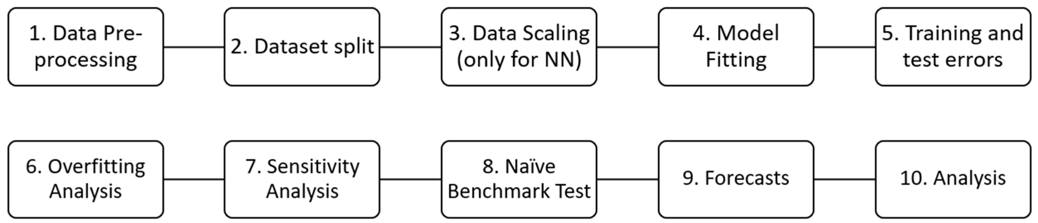
Given the uncertainty surrounding the future levels of CO₂ emissions from buildings, novel methods based on machine learning can be used as forecasting tools. These methods provide fundamental insights into the future evolution of CO₂ emissions while taking into account the efforts made so far. This work aims to provide insights into the future level of CO₂ emissions from buildings in different countries. This section presents the ten-step machine learning methodology, which is illustrated in Figure 1 below.

This methodology can use any machine learning methodology. In this paper, we have chosen to use linear regression, ARIMA, shallow neural networks, and deep neural networks (also known as “deep learning”) as these fundamental algorithms have not been used before in the context of CO₂ emissions from buildings. However, note that the methodology is expandable to any number and type of algorithms.

In a linear regression model, the relationship between the target variable and the independent variable x is expressed in the form $y=\alpha +{\displaystyle \sum }_i{b}_i{x}_i+ ϵ$, where $\alpha$ is the intercept that expresses the predicted value for the target variable when all the predictor variables $x_i$ are equal to zero. Additionally, $x_i$ are the features (or predictors), and $y$ is the target, which, in this case, is linearly related to the features. Finally, $b_i$ are the regression coefficients, which multiply the predictor variables, and each of them can be interpreted as the change in the predicted value for the target variable for each unit change in the specific regression coefficient, provided that all other regression coefficients remain constant. To fit the linear regression model to the training set, the ordinary least squares (OLS) methodology is used to obtain the optimal value for the parameters (intercept and coefficients). Specifically, the OLS is an optimization method that minimizes the standard loss function, which for the case of linear regression is equal to the sum of the squared residuals, as in ${\displaystyle \sum }_i^N{\left(y_i-\widehat{y_i}\right)}^2$, where $y_i$ is the actual value for observation $i$ and $\widehat{y_i}$ is the predicted value, while N is the total number of observations in the estimation sample.

ARIMA (autoregressive integrated moving average) is a machine learning algorithm for making forecasts. One of the hyperparameters includes the autoregressive (AR) term, also known as the “lag order”, which represents the number of lag observations. Another hyperparameter is the differencing order I, known also as the degree of differencing, and represents the number of times that the raw observations have differed. Finally, the moving average (MA) term represents the size of the moving average windows. Note that a hyperparameter, as opposed to a parameter, attains its value as set by the user and is not the result of an optimization algorithm. Note that the model equation is determined by the auto-regressive (AR) order. In this case, the model equation for a k-order ARIMA model takes the following form: $y=\alpha +b_1{x}_1\left(t\right)+{\displaystyle \sum }_i{b}_i{x}_i\left(t\right)+{\displaystyle \sum }_k{\theta }_{k}y\left(t-k\right)+ϵ\left(t\right),$ where $ϵ\left(t\right)~N\left(0,{\sigma }^2\right)$ and $\alpha$ is the constant or intercept. ${\theta }_k$ is the k-order autoregressive coefficient, and ${\sigma }^2$ is the variance of the error term, where $x_i$ are the independent variables.

Note that there are three steps for model building in ARIMA [23]. The first step is the identification step. This includes checking for stationarity with tests such as the KPSS test (Kwiatkowski-Phillips-Schmidt-Shin), which states that a time series is stationary when the corresponding p-value is greater than the selected significance level. In this step, methods such as auto ARIMA or the ACF/PACF plots are utilized to determine the optimal ARIMA order. The second step includes the model estimation or fitting, where the model is trained on the training set. Finally, the last step includes conducting diagnostic tests. Such tests make sure that the three key assumptions of ARIMA are satisfied, namely that the residuals are serially uncorrelated (via the Ljung-Box test), have constant variance (i.e., no heteroskedasticity), and are normally distributed (via the Jarque-Bera test).

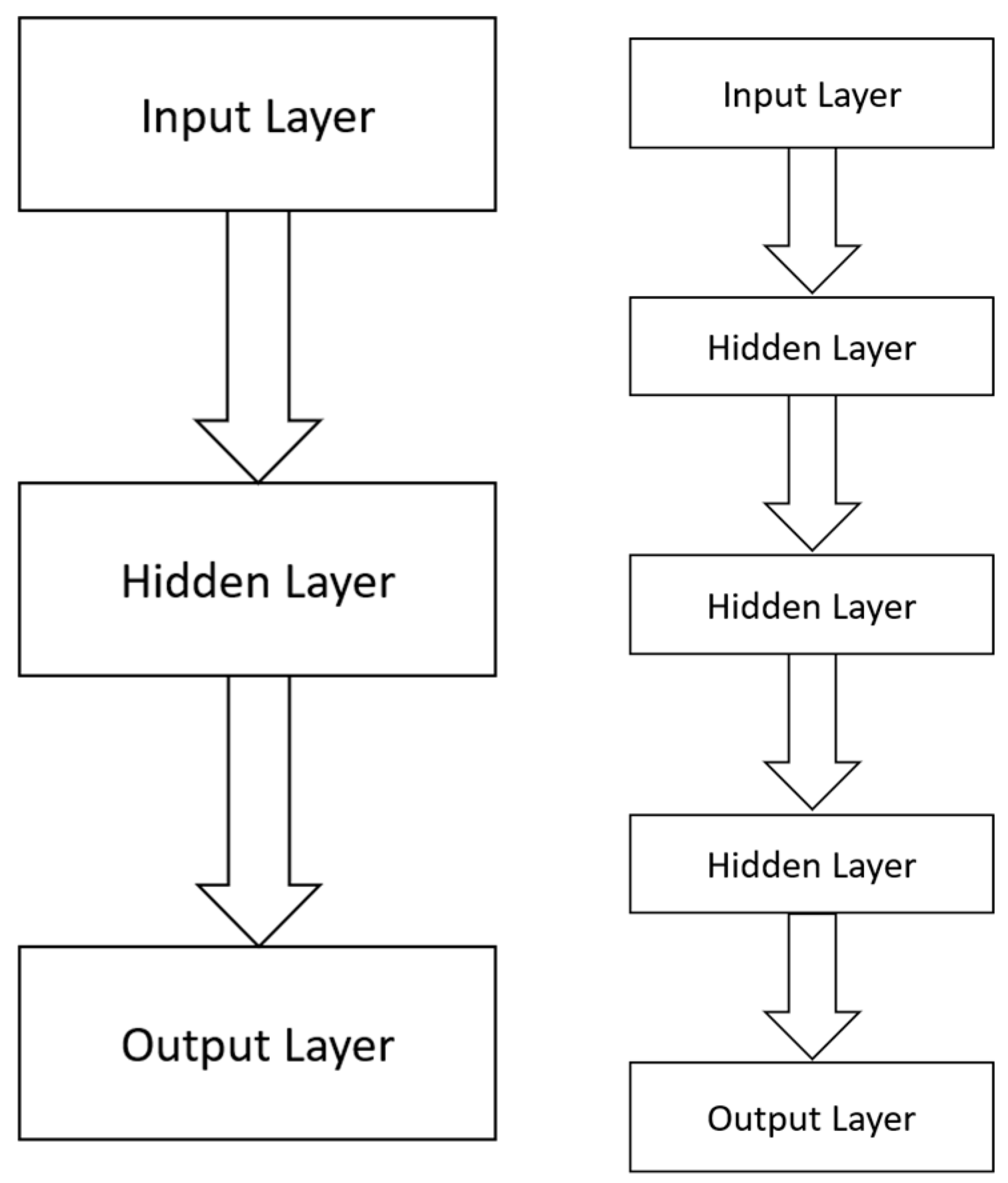
Neural networks constitute a forecasting modeling approach with two main types: shallow and deep, as shown in Figure 2. The former is a type of neural network with a single hidden layer, while the latter is a neural network with multiple hidden layers. Once a neural network model is fitted to the training set, an optimization method is applied, typically gradient descent, to yield the optimal values of the parameters, which are weights and biases. Key hyperparameters typically include the number of layers, the number of neurons per hidden layer, the activation function, the number of epochs, the learning rate, and the batch size. Linear activation functions typically characterize output layers, while nonlinear ones (such as the rectified linear unit) characterize hidden layers. The learning rate determines the update of the parameter values at every gradient descent step, where “gradient” is the first derivative of the loss function with respect to the parameters. That is, the learning rate determines by how much the parameters should change at each gradient descent step and takes values in (0,1). The batch size is the size of the subset of the training set that is used for each iteration (or step) of gradient descent for each parameter update. Finally, the number of dense layers represents the depth of the network; the greater the number of dense layers, the deeper the network, while the number of hidden units (or neurons) in each (dense) layer represents the width of the network; the more neurons, the wider the network. In general, deeper (rather than wider) networks perform better; however, having too many layers or too many neurons can potentially lead to overfitting.

Regarding the methodology, as mentioned, it consists of ten steps, all of which collectively lead to the generation of forecasts from models with acceptable accuracy and no overfitting. The steps are as follows:

The first step is called “Data Preprocessing”, and it involves the selection and processing of data. In this case, the World Bank is the source of the data selected for this work, and the data consist of annual CO₂ emissions from buildings, expressed as a percentage of total fuel combustion. Note that the focus is not on CO₂ emissions in general but specifically on CO₂ emissions related to the building sector. It was particularly challenging to obtain such data, with the World Bank being the only available source. Specifically, the data cover the period from 1971 to 2014, and there is a single value for every year, which is the annual-average level of CO₂ emissions. As such, the dataset consists of 44 observations, which may make it challenging to produce high-accuracy forecasts given that the larger a dataset is, the more likely it is to obtain significant forecasting errors. Still, we have chosen to conduct the analysis because the size of the dataset does not guarantee low accuracy in the results. In addition, the methodology presented remains valid and unchanged irrespective of the size of the dataset. Therefore, there is merit in presenting it, particularly given that it is the first time that it finds application to such a dataset.

The second step involves the definition of the feature, the feature matrix, the target variables, and their components. These components include the training, testing, and validation components. However, when the datasets are small (e.g., with fewer than 100 observations), there is no room for creating a validation component. For this reason, we have split the original dataset into a training subset and a test subset without defining a validation subset. This is because there are only 44 values in the original dataset, so the training subset would only have about 20 values, which could affect the efficiency of model fitting. On the other hand, when a validation subset is not included, the training subset comprises 36 values, making it a superior alternative. Note that the use of a validation set in the analysis is aimed at fine-tuning the hyperparameters, but this fine-tuning can also be approximated through the sensitivity analysis performed in Step 7 of this method.

The third step applies to shallow and deep neural networks and involves scaling the feature matrix and the target variables, as well as their component/subset matrices (training and test set components). Note that this step is not necessary, and therefore omitted, for linear regression or ARIMA. The resulting scaled matrices are used to produce scaled predictions and scaled forecasts, as described in subsequent steps of the methodology, as this is a necessary part of the function of neural networks. Later, the scaled values will be unscaled again to obtain the actual results (predictions and forecasts).

The fourth step involves model fitting, also known as a model estimation. Specifically, the models are fitted to the training set, so that they can learn the patterns held in the training dataset and then be able to use this learning for generating predictions and forecasts. This is a case of univariate model fitting, meaning that the models for each of the regions are fitted to the datasets of the corresponding regions and not to datasets from other regions. Therefore, for the eight regions/datasets considered in the model, eight models are fitted, per algorithm (linear regression, ARIMA, shallow neural networks, and deep neural networks), resulting in 32 fitted models in total.

The fifth step involves calculating the training and test set predictions. The former are the outputs of the model corresponding to the training dataset, i.e., the period 1971–2005, while the latter are the outputs of the model corresponding to the test dataset i.e., the period 2006–2014. Then, by comparing these predictions with the original training and test subsets (i.e., the actual values belonging to the datasets obtained from the World Bank), it is possible to evaluate the corresponding errors known as “mean absolute percentage errors”, or MAPE. These errors express the distance between the outputs of the models (i.e., the predictions) and the actual values, thereby reflecting the model accuracy in seen (i.e., the training set) and unseen datasets (i.e., the test set).

The sixth step involves the overfitting analysis. Specifically, the training and the test errors are compared with each other and if their difference is greater than 10%, the corresponding model is considered to be overfitting. Overfitting can happen when the training set errors are small, which indicates very good fitting, while the test set errors are very large, indicating very high test errors, i.e., poor model performance on unseen data. In other words, when a model overfits, it has learned from the training set data so well (i.e., has very small training set errors) that it cannot generalize to new, unseen data, resulting in significant test-set errors. For this reason, such a model cannot be utilized to determine forecasts; it is disqualified from further analysis.

The seventh step constitutes the sensitivity analysis of the test set errors. Specifically, for different combinations of hyperparameters, the test errors are evaluated. This analysis is conducted because it can offer significant insights into the model’s performance on the forecasts. Particularly, the test set errors are considered proxies for the forecasting errors because both are errors on unseen datasets and reflect the model’s performance on new data. Therefore, the sensitivity analysis can provide significant insights into the behavior of the forecasting errors themselves.

The eighth step involves conducting the naïve benchmark test. While the overfitting analysis focused on the comparison between the training and test errors, the naïve benchmark test focuses solely on the test error. It involves comparing the test error of the model used in the analysis against the test error of a “naïve” or simple model. The idea is that if the naïve model can yield a smaller test error, then the test error of the model used in the analysis is considered unacceptably high. This test allows characterizing whether a test error is high or not, as the naïve model serves the purpose of the benchmark for this comparison.

The ninth step involves the generation of the forecasts and the corresponding graphs. Note that forecasts are the outputs of the models corresponding to the forecasting period, i.e., the years until 2050. Note that at this point the forecasts are produced only by those models that have successfully passed both the overfitting test and the naïve-model benchmark test. As a result, the models that will be used for the generation of the forecasts are guaranteed not to overfit (since they have successfully passed the overfitting test) and to have a relatively low forecasting error since they have successfully passed the naïve-benchmark test.

Finally, the last step incorporates the analysis of the results obtained in the previous steps. Specifically, this step includes the comparison of the model performance in terms of overfitting as well as test-set errors (test-set MAPE) and a description of the final selection of the models whose forecasts will be accepted based on the results of the naïve—model tests and of the overfitting tests.

3. Literature Review on Machine Learning Algorithms

A machine learning model is an algorithm that learns, by itself, the pattern in the data and develops the relationship between the dependent variable, or target, y, and the independent variables, or features, x, as in y = f(x) + $ϵ$, where $ϵ$ is the error term. Machine learning models have constituted fundamental algorithms for making forecasts, such as linear regression, ARIMA, and neural networks, as discussed in the previous section.

To the best of our knowledge, these algorithms have not yet been applied in the context of producing forecasts on the dataset for CO₂ emissions from the building sector. This fact alone renders this work novel since it demonstrates for the first time such an application.

Linear regression has found application in other areas, such as electricity revenue forecasting [24], data-driven power flow modeling [25], and the prediction of electricity consumption [26,27].

Regarding ARIMA, it has found application in other cases such as the prediction of next-day electricity prices [28], the development of stochastic wind power modeling [29], the solar PV forecast for the optimal charging of electric vehicles (EV) at the workplace [30], as well as the prediction of road gradient and vehicle velocity for hybrid electric vehicles [31].

Regarding neural networks, they have found applications in cases such as solar power forecasting [32] and electricity price short-term forecasting [33,34]. They have also been used to generate forecasts of CO₂ emissions in Bangladesh until 2019 [35], in China until 2030 [36], and globally until 2019 [37].

As can be seen, none of the above works includes the application of machine learning to data on the CO₂ emissions from buildings, nor does it present a step-by-step methodology as it is conducted in the current work. In this context, the novelty of the presented work is as follows:

• For the first time in the literature, a ten-step methodology based on machine learning algorithms for the generation of accurate forecasts is described. This methodology is constructed in such a way that it is dataset-independent (i.e., it is not restricted only to data for CO₂ emissions) and it is expandable (i.e., new algorithms can be included, and it is not restricted only to the algorithms presented here, i.e., linear regression, ARIMA, and neural networks).
• Application: for the first time in the literature, the ten-step methodology is applied to a dataset on CO₂ emissions specifically related to the building sector and across multiple regions across the world.
• Presentation of a comprehensive comparison of linear regression, ARIMA, shallow neural networks, and deep neural networks based on a wide range of metrics and sensitivity analyses.

4. Case Study

In the previous section, it was stated that the aforementioned machine learning algorithms can be used for conducting forecasts. This section presents the application of these algorithms to forecasting CO₂ emissions from the building sector across different regions of the world.

4.1. Setting up the Studies

The first step of the analysis includes the data preprocessing stage. This stage consists of selecting the dataset of interest, as per

Table 1. Dataset of CO₂ emissions from buildings, expressed as a percentage of total fuel combustion, in Brazil (BRA), India (IND), China (CHN), South Africa (ZAF), the United States (USA), Great Britain (GBR), the world (WLD), and EUU (the European Union), covering the period between 1971–2014.

Year	BRA	IND	CHN	ZAF	USA	GBR	WLD	EUU
1971	7.04	15.08	21.59	7.92	19.06	17.23	18.61	21.95
1972	7.05	14.03	21.32	7.74	18.39	18.14	18.43	22.12
1973	6.56	14.18	20.83	6.94	17.04	17.42	17.56	21.89
…	…	…	…	…	…	…	…	…
2012	4.75	5.70	5.30	5.55	9.71	20.13	8.64	16.34
2013	4.51	5.70	5.30	5.59	10.68	20.82	8.80	17.06
2014	4.29	5.49	5.35	5.47	11.01	19.06	8.59	15.46

, from a reliable source [38], across geographical locations of interest as well as the timeline. In this case, the dataset includes the CO₂ emissions from the buildings sector across different regions in the world (Brazil, India, China, South Africa, the United States, Great Britain, the world, and the European Union) between 1971–2014. The objective of the analysis is to make forecasts for the timeline from 2015–2050.

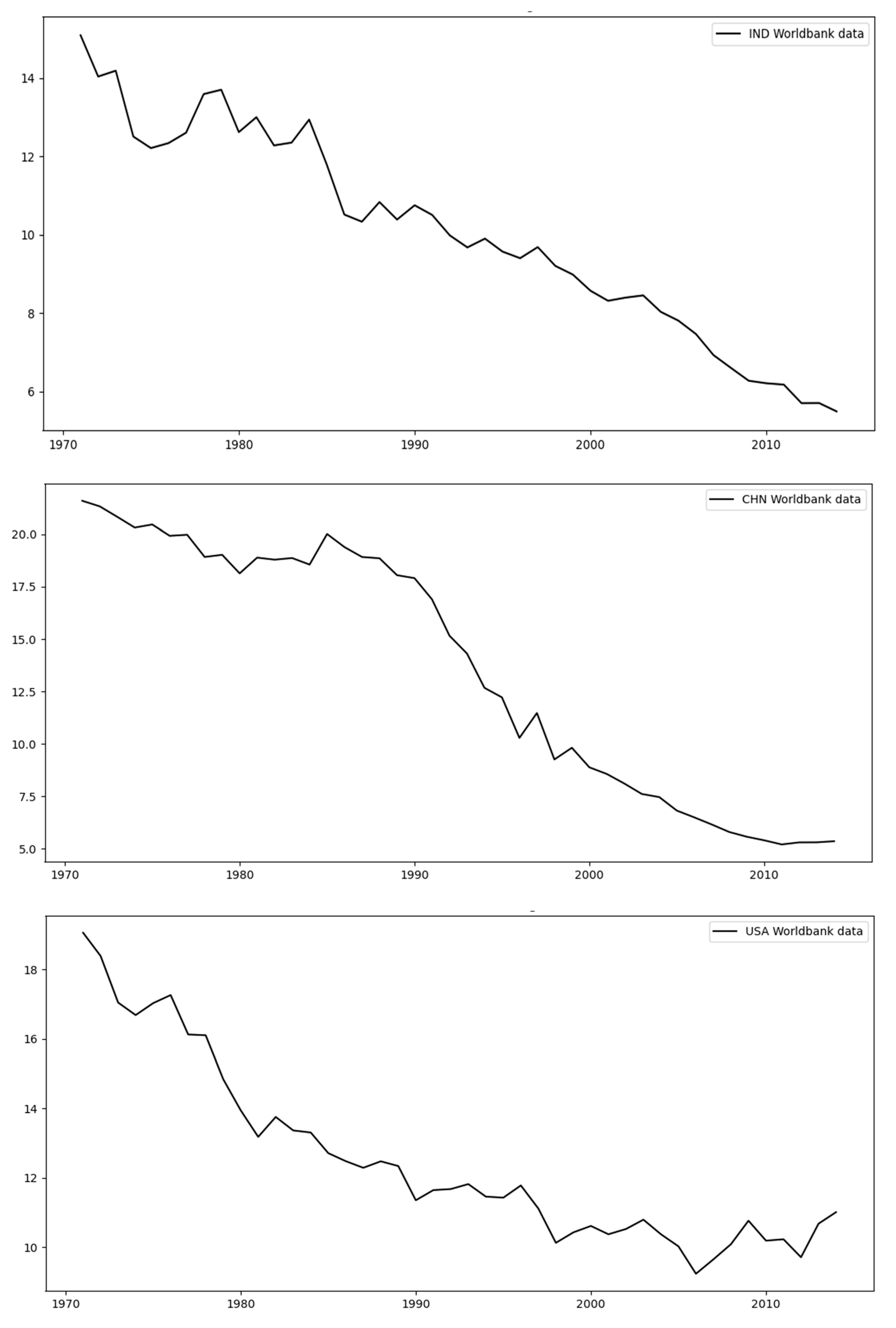
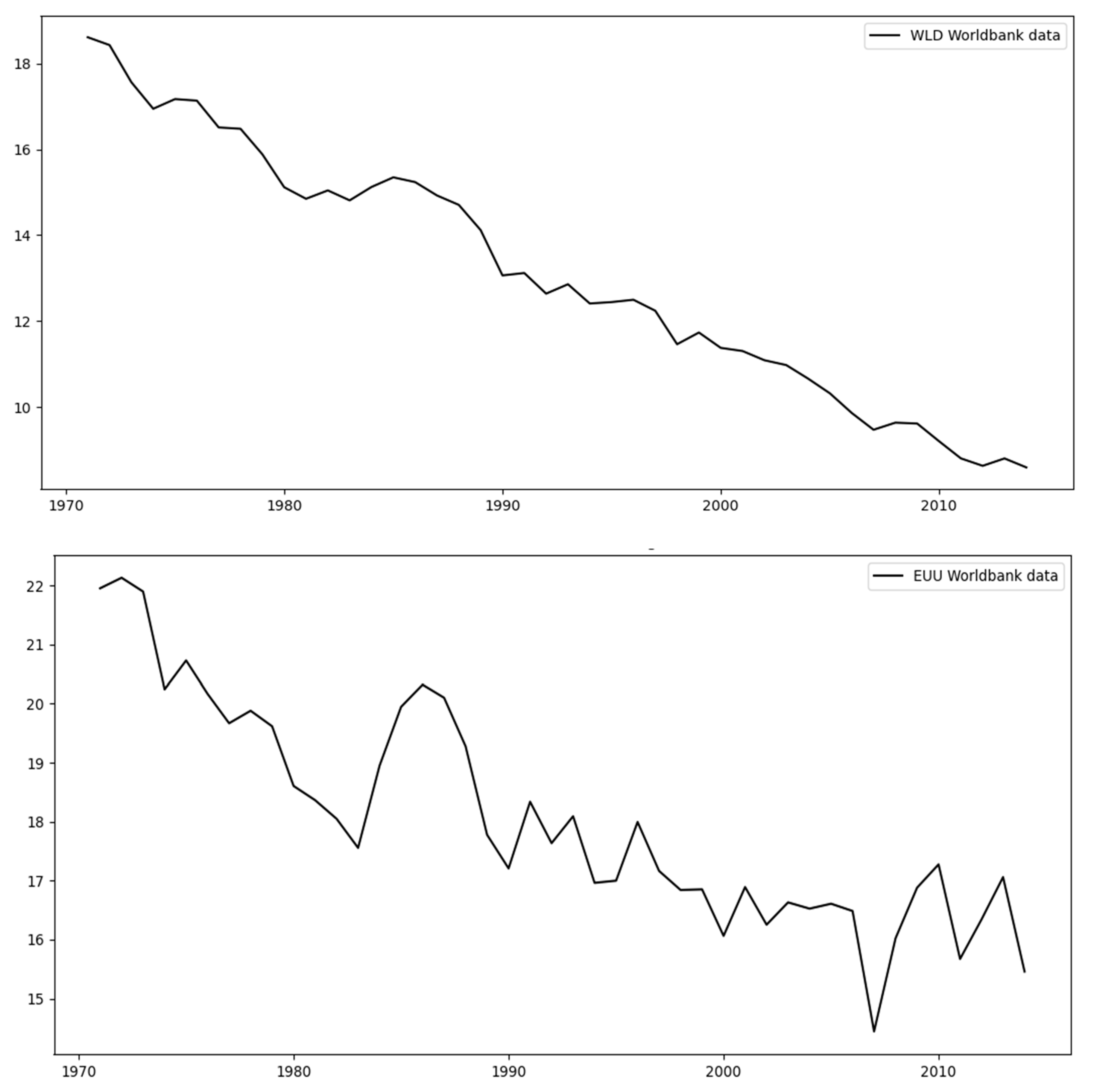
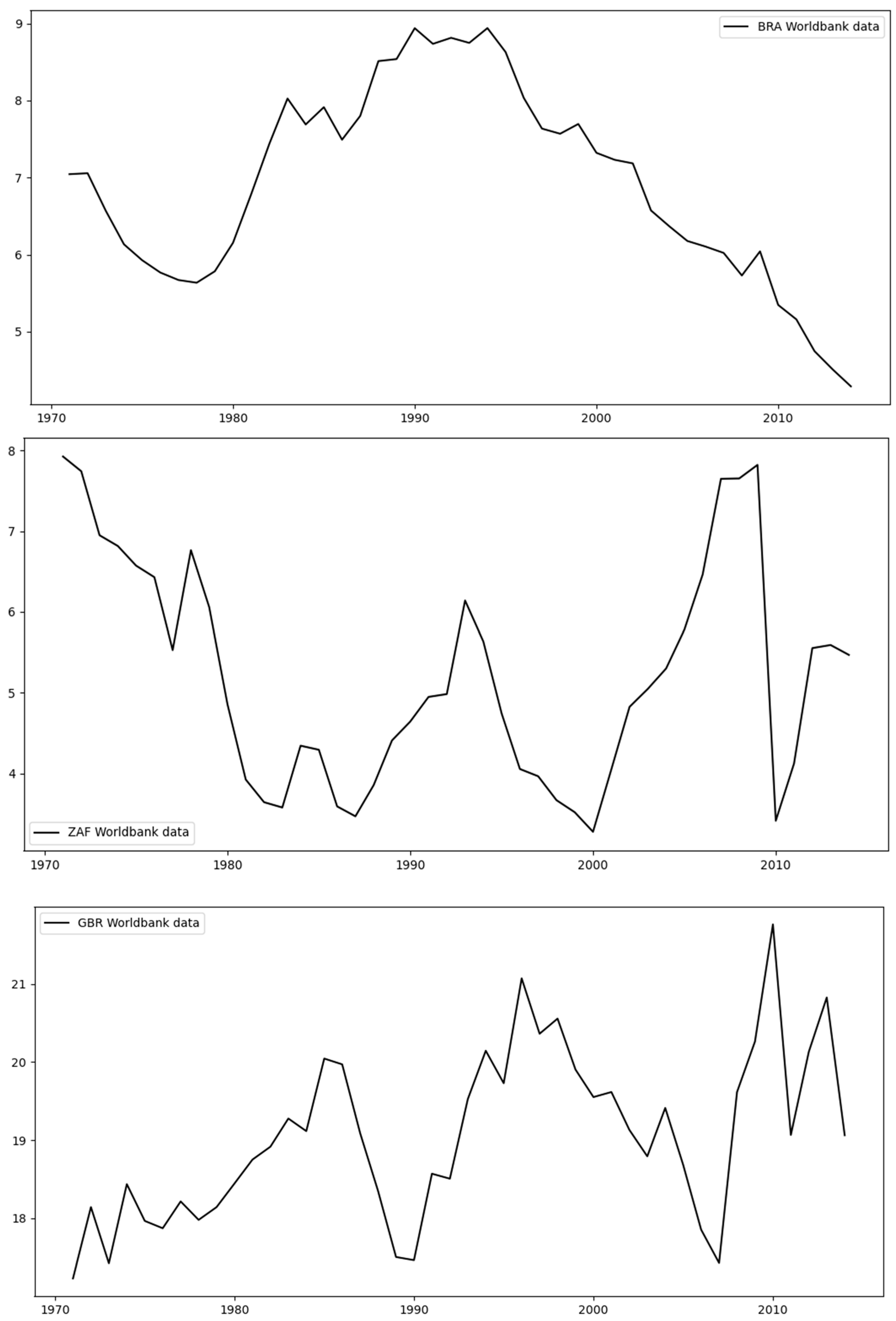
Figure 3 and Figure 4 below show the original data for each of the different regions considered in this study. By observing these data, we can determine that there are two main types of regions: those with a relatively small variability (Figure 3) and those with high variability (Figure 4). 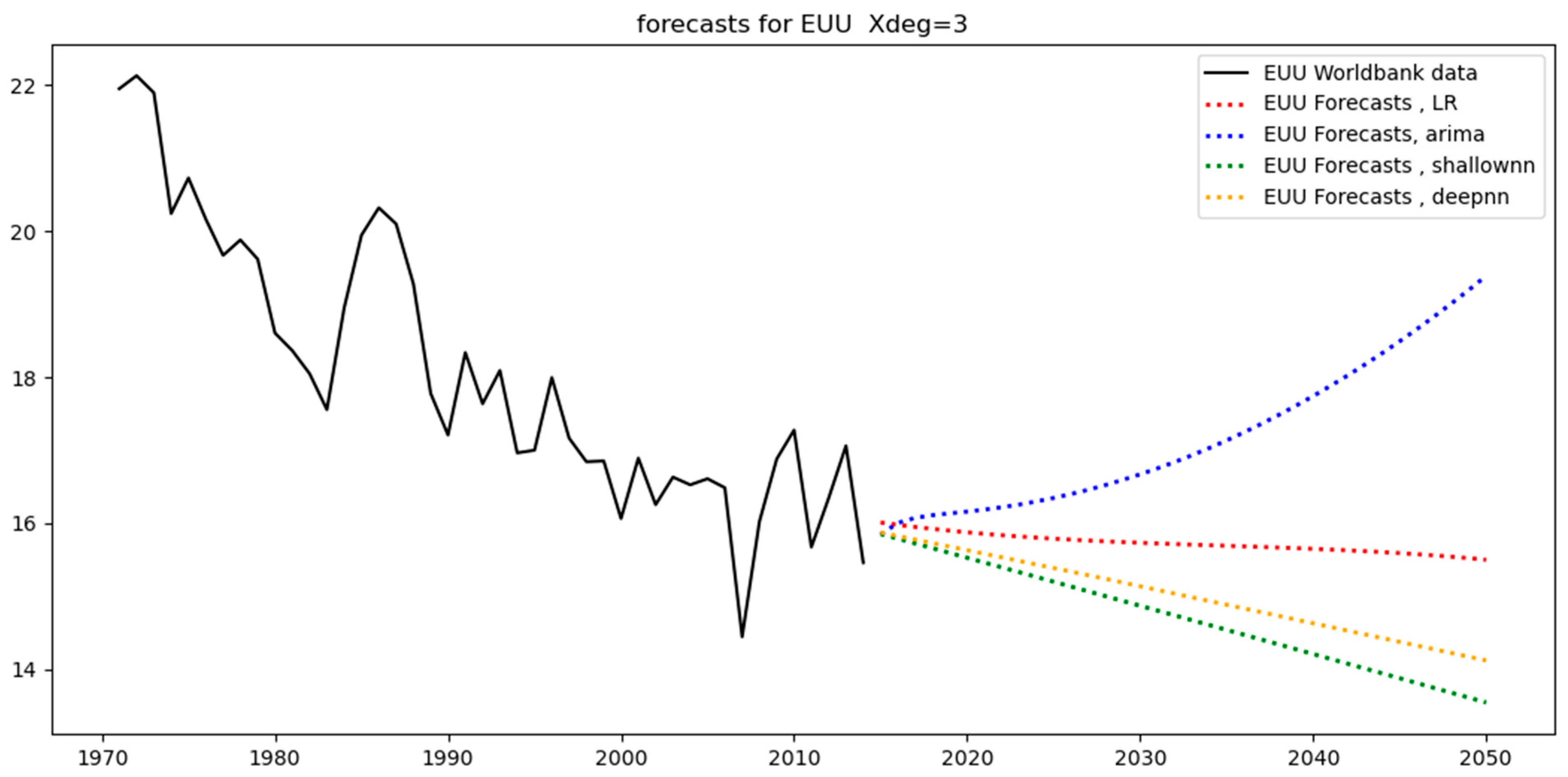The first set includes the regions India (IND), China (CHN), the USA, the World (WLD), and the European Union (EUU), as can be seen in Figure 3 below; these datasets follow straight trends with some fluctuations, with WLD exhibiting the smallest amount of fluctuation as opposed to that for EUU.

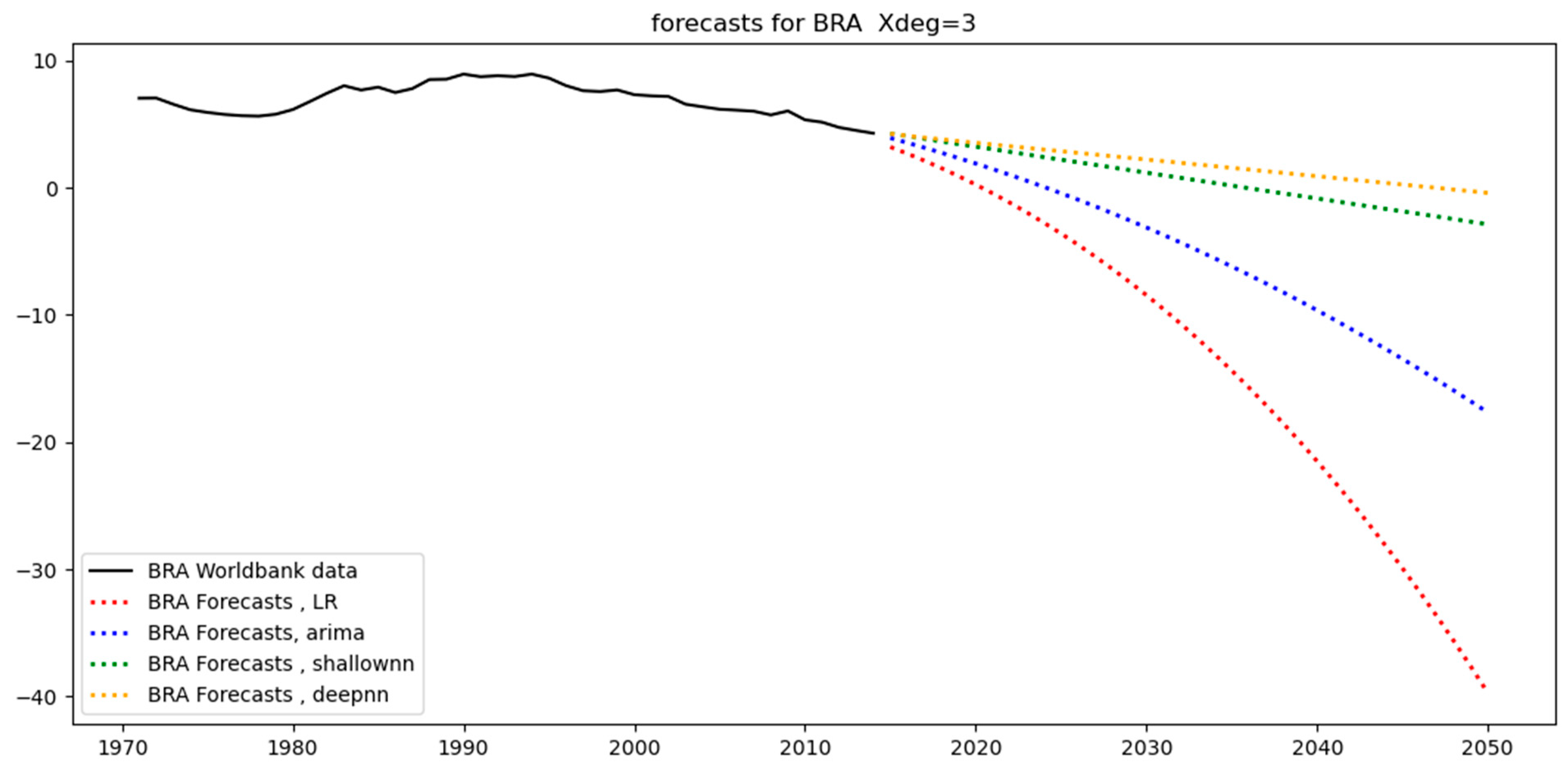
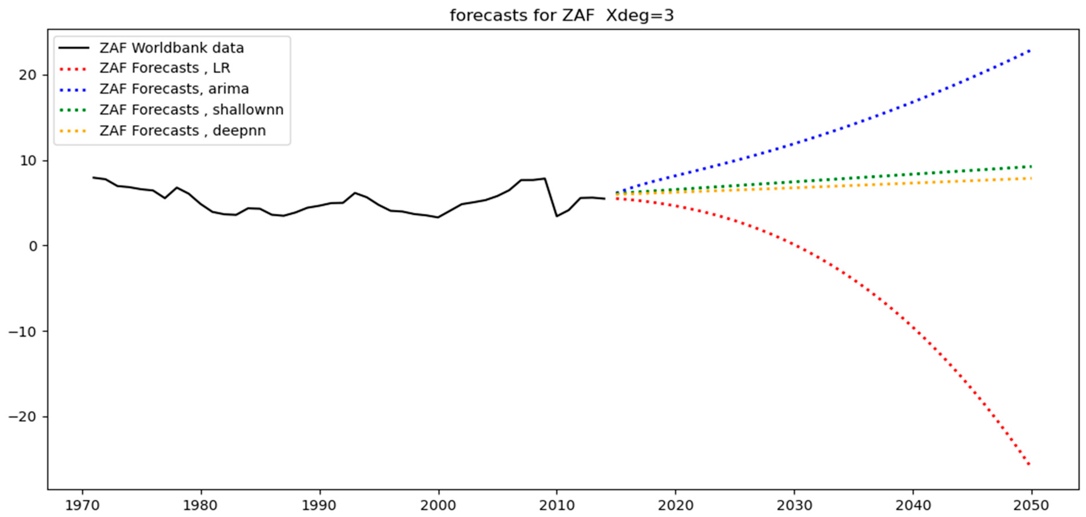
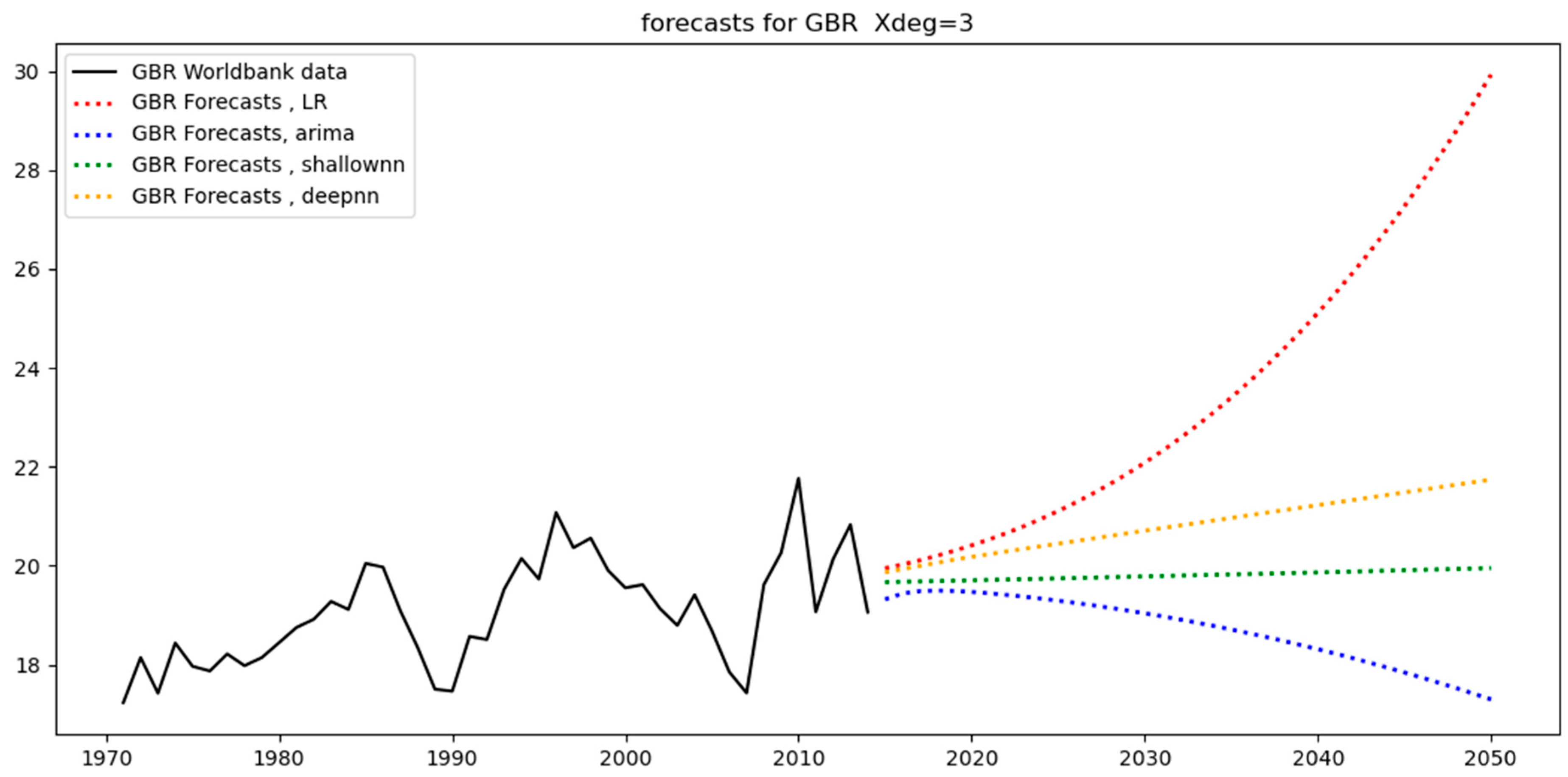
The second set includes the regions of high variability, which are Brazil (BRA), South Africa (ZAF), and Great Britain (GBR), as can be seen in Figure 4 below. We can observe that BRA has a peak around 1991 with an overall parabolic trend, while ZAF and GBR have significant variance.

The next step is to add polynomial features to the model. We consider a third-degree feature matrix for the existing dataset as well as for the forecasting dataset. Having a third-degree polynomial allows one to capture non-linearities in the dataset and produce a more accurate forecast. Furthermore, the original dataset, which consists of 44 observations (1971–2014) for each region, is split into a training set and a test set. The former is selected from approximately 80% of the original dataset, i.e., 35 observations, with the remaining nine forming the test set.

Subsequently, the features matrix as well as the target variables are scaled, which is necessary for the neural network algorithms, while ARIMA and linear regression do not require scaling but, rather, continue using the unscaled versions of the matrices.

Moreover, all models across all regions are fitted to the training sets. Since there are eight regions in total, there are eight training sets and, as a result, eight fitted models in total. Specifically, the ARIMA models are of the order (1,0,0). The first order being equal to one means that y(t) is modeled as a function of y(t − 1). The second order (known as the integration order) being zero means that the model predicts y(t) directly; if it was equal to 1, then the model would predict the first difference of y(t), which is $y\left(t\right)-y\left(t-1\right)$ symbolized as $\mathsf{\Delta }y\left(t\right)$. The third order (known as the moving average order) being 0 means that the model predictions do not take into account the previous errors; the error is defined as $ϵ\left(t\right)=y\left(t\right)-\widehat{y}\left(t\right)$, where y(t) is the true value of the time series and $\widehat{y}\left(t\right)$ is the value predicted by the model. If the MA order was set equal to one, then the model would predict y(t) as a function of $y\left(t-1\right)-\widehat{y}\left(t-1\right)$, which is symbolized as $ϵ\left(t-1\right)$ [39,40]. For the ARIMA models, too, the Jarque Bera test is run. As can be seen in

Table 2. The p-value of the Jarque Bera Test for the selected regions.

Region	p-Value
BRA	35%
IND	84%
CHN	85%
ZAF	18%
USA	70%
GBR	73%
WLD	39%
EURO	43%

, it yields p-values greater than 10% (the default significance level) for ARIMA models applied to every region. This indicates that the model residuals are normally distributed (i.e., the null hypothesis that the model residuals are normally distributed is not rejected), which is the desired result and reflects the efficiency of the fitting process.

In terms of neural networks, we define and fit eight shallow neural network models and eight deep neural network models, each for each of the eight regions. The activation function for every hidden layer is the rectified linear unit, which has been shown to have the best performance on most learning tasks [41]. This is why the activation function for the output layer is linear. We have also selected as hyperparameters 100 neurons for every hidden layer, 100 epochs for the optimization method, which is stochastic gradient descent, and a batch size equal to eight. These hyperparameters have been selected following sensitivity analyses to ensure that the model does not overfit.

At this point, all the models have been defined in terms of their hyperparameters and have been fitted to the training set. The next subsection explores the predictions obtained.

4.2. Predictions

In the previous subsection, the linear regression, ARIMA, and neural network models for each region were fitted to the training sets. Since the models have now been trained, the next step is to proceed with the calculation of the predictions on both the training and test sets. The training- and test-set predictions are the outputs of the models derived from their application to the training and test sets.

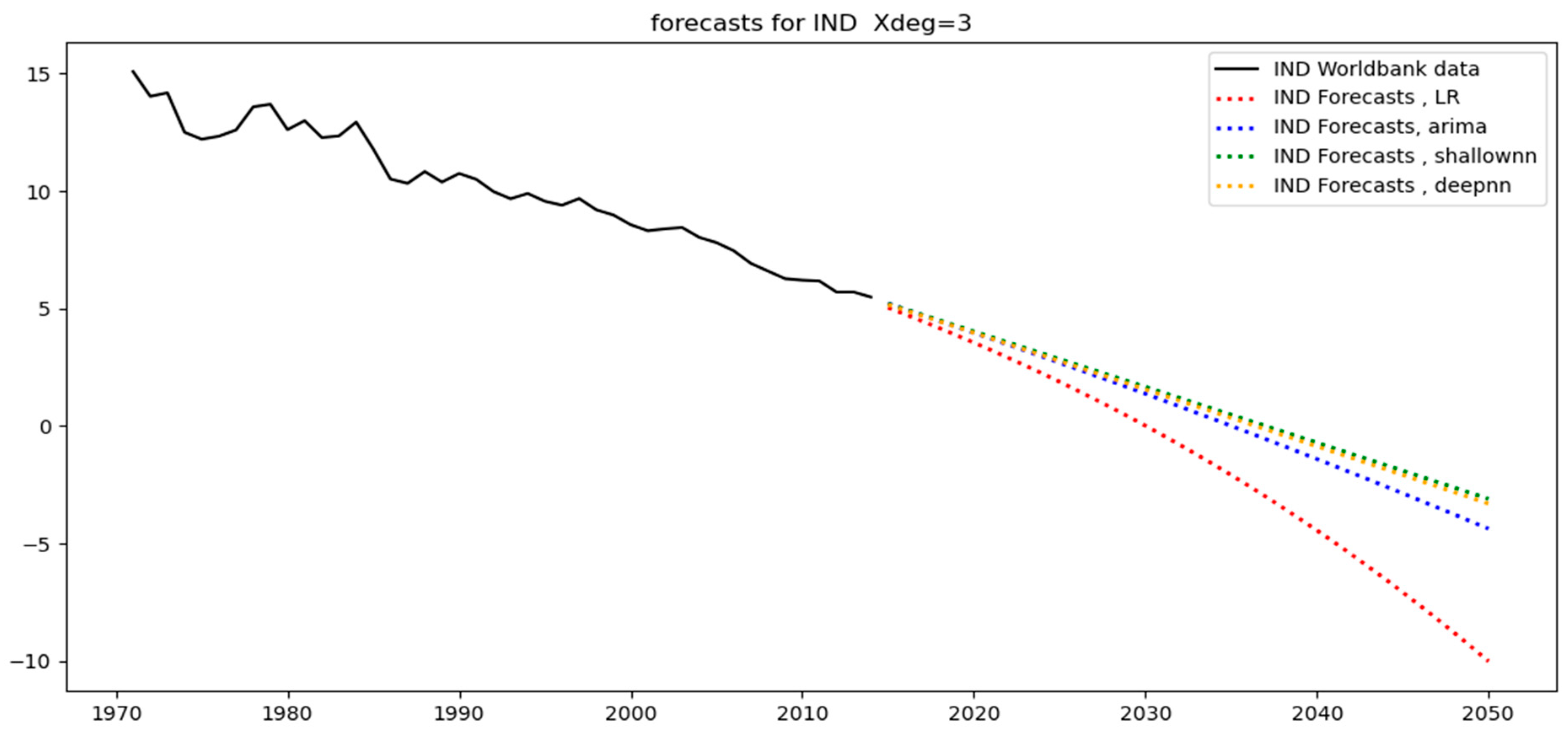
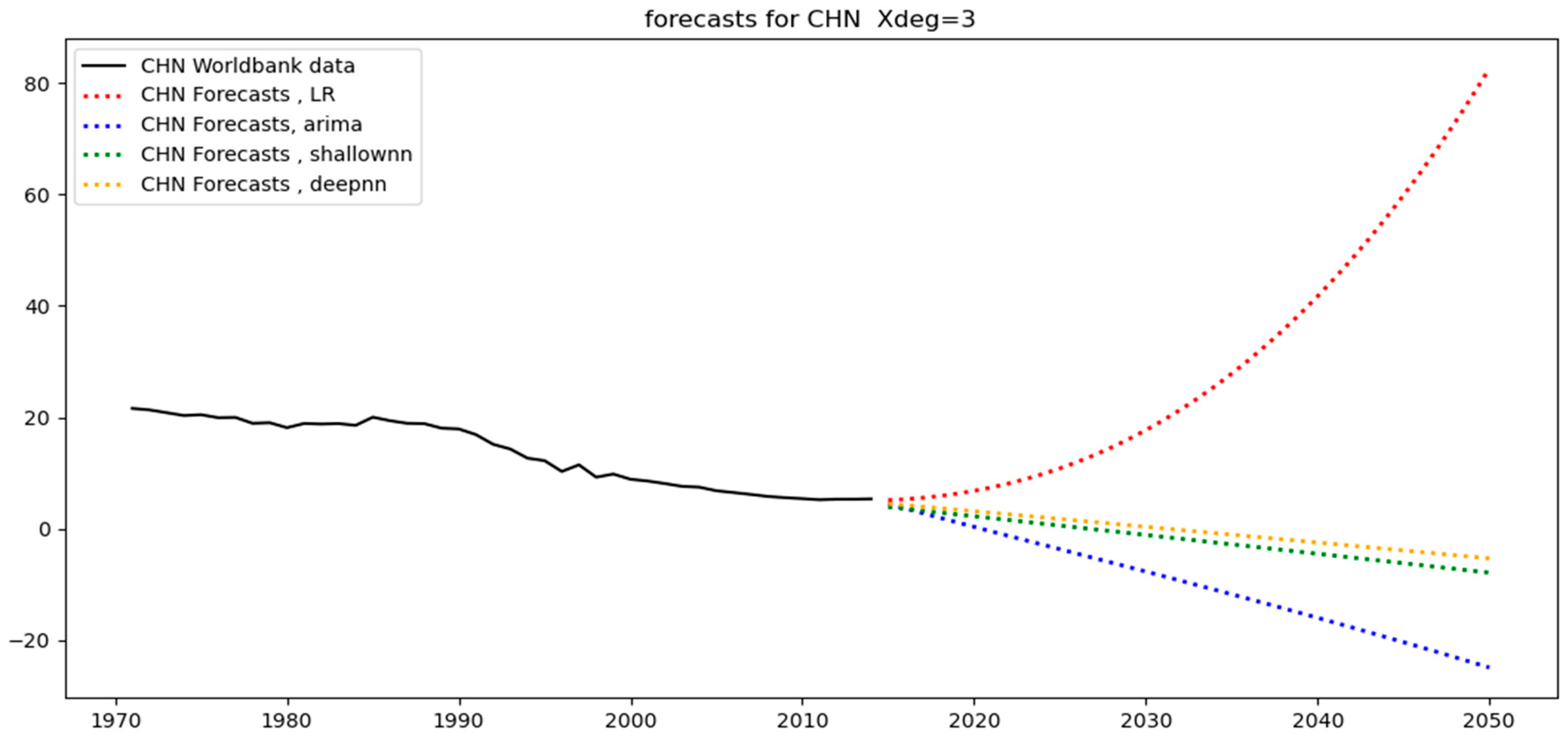
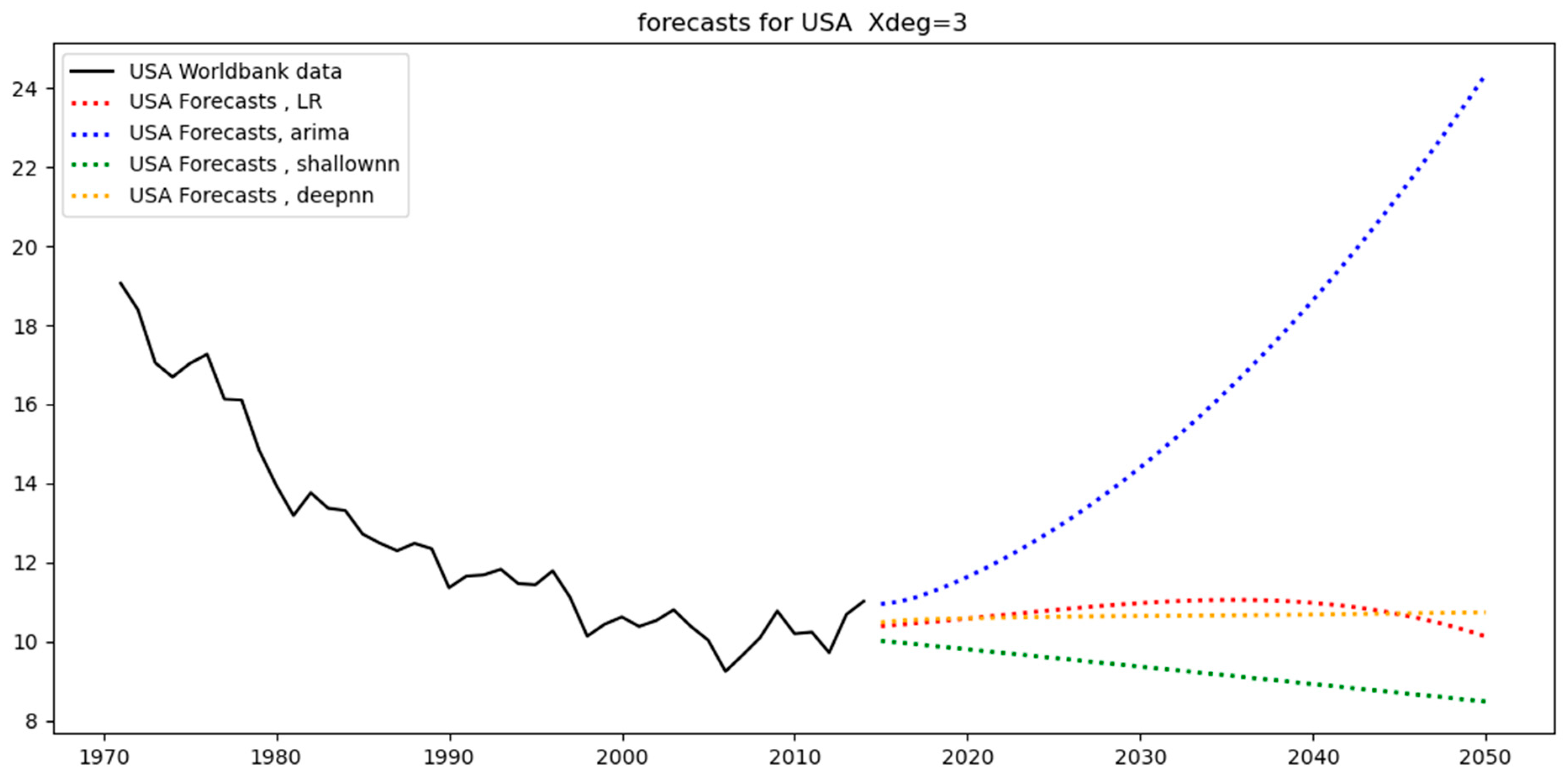
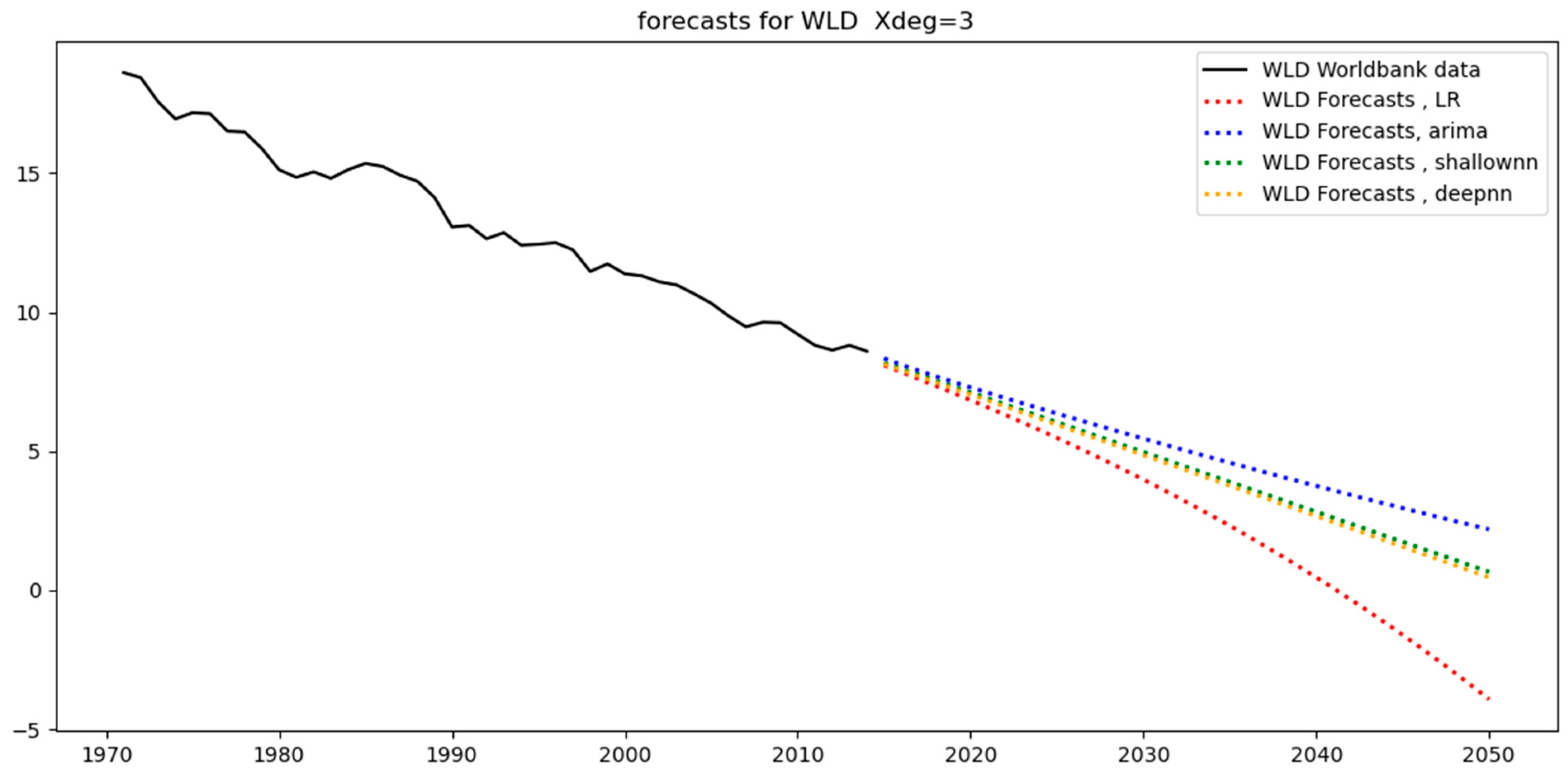
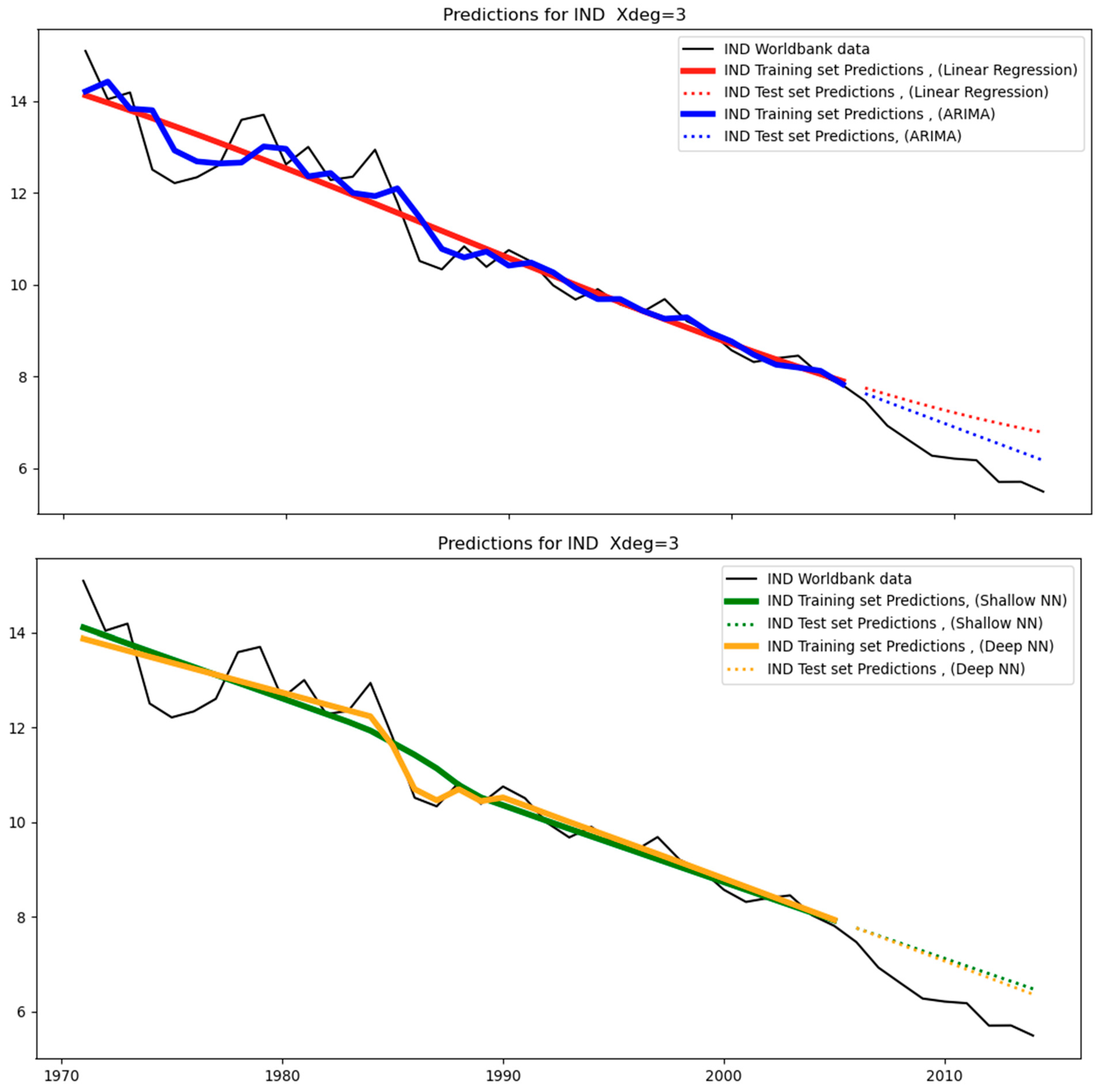
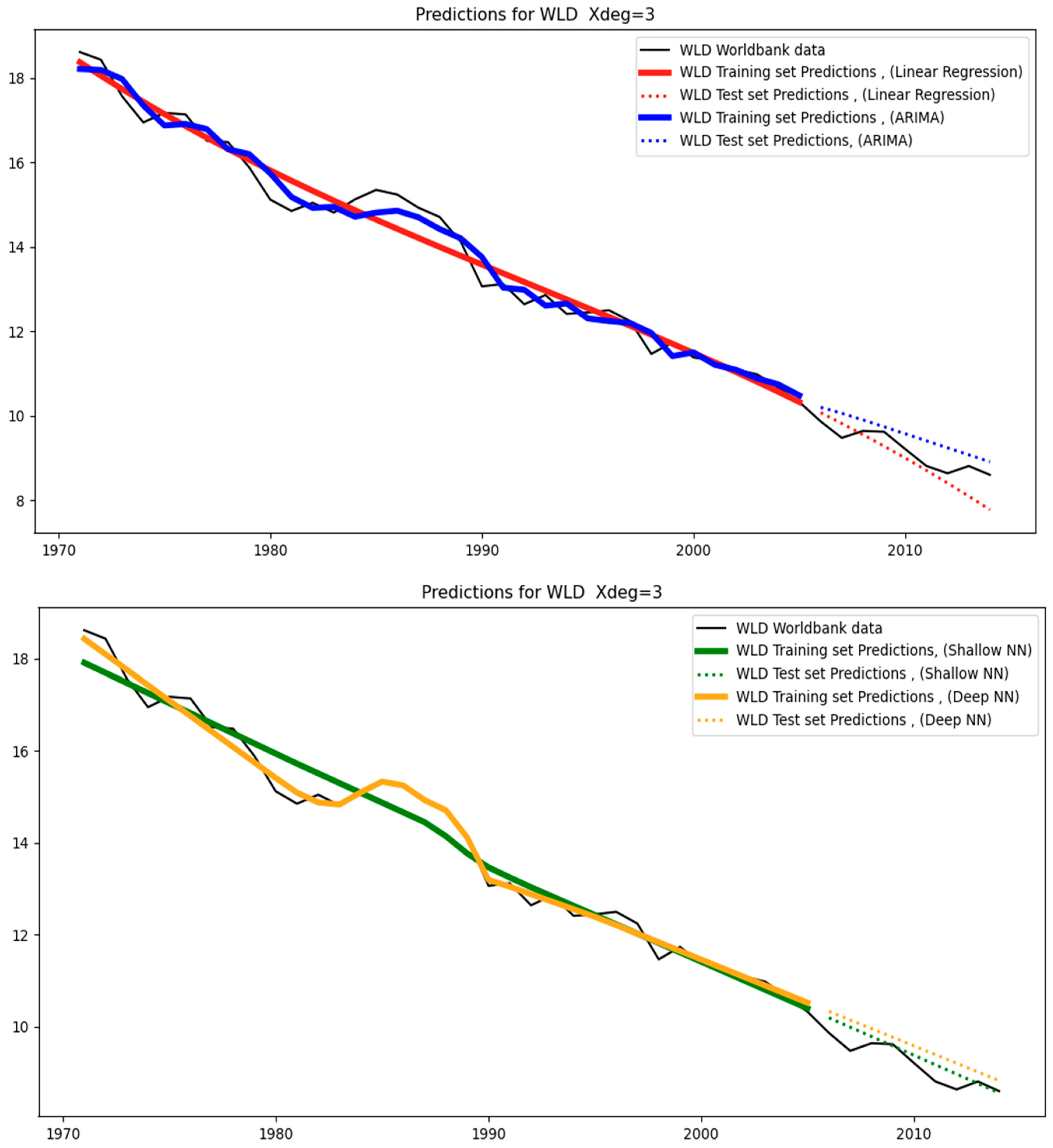
Figure 5, Figure 6, Figure 7, Figure 8, Figure 9, Figure 10, Figure 11 and Figure 12 below show the models’ predictions using a third-degree polynomial (Xdeg = 3). The black straight lines are the original data. These are the counterfactuals against which the predictions are compared. The straight-colored lines are the training set predictions (covering the period 1971–2005), while the dotted colored lines are the test-set predictions (covering the period 2006–2014). Different colors characterize different models (for example, ARIMA models are shown in blue).

From a close observation, we can see that the test-set predictions (i.e., dotted colored lines) are less aligned with the test-set data (i.e., black straight line covering the period 2006–2014) than the training-set predictions (i.e., straight colored lines) are aligned with the training-set data (i.e., black straight line covering the period 1971–2014). This happens because the test set essentially constitutes unseen data for the models as opposed to the training set data, where the models were trained. As a result, it is expected that the level of divergence between the straight-colored lines and the black line will be less than that between the dotted-colored lines and the black line. The level of divergence is also known as the “error”: training-set error and test-set error, respectively.

4.3. Prediction Errors and Overfitting Analysis

As mentioned in the previous subsection, the level of divergence between the predictions and the actual data are known as the “prediction error”. If the models have not been trained effectively, then the test-set error will also be high, leading to a reduction in accuracy.

Specifically, to assess the effectiveness of the fitting process, we evaluate the mean absolute percentage error (MAPE) on both the training set and the test set, as shown in the following tables.

Table 3. The mean average percentage error (MAPE) on the training set, per region and model, is under a polynomial degree of three.

Region	Linear Regression	ARIMA	Shallow NN	Deep NN
IND	3.45%	3.45%	3.26%	2.82%
CHN	6.30%	6.71%	3.66%	2.13%
USA	2.44%	2.94%	2.50%	2.06%
WLD	2.10%	2.13%	2.06%	1.06%
EUU	3.06%	3.03%	3.16%	1.45%
BRA	5.73%	8.19%	4.10%	2.59%
ZAF	12.99%	13.05%	12.53%	7.44%
GBR	2.74%	2.84%	2.75%	1.15%

shows the MAPE on the training set (also known as the training-set MAPE), while

Table 4. The mean average percentage error (MAPE) on the test set, per region and model, is under a polynomial degree of three.

Region	Linear Regression	ARIMA	Shallow NN	Deep NN
IND	15.68%	10.07%	13.72%	12.75%
CHN	74.74%	89.69%	44.35%	28.47%
USA	8.52%	8.36%	8.67%	8.32%
WLD	3.79%	4.20%	2.38%	4.33%
EUU	11.02%	4.36%	4.87%	4.45%
BRA	93.01%	2.17%	4.49%	5.59%
ZAF	25.48%	38.84%	24.22%	25.85%
GBR	10.53%	5.73%	5.50%	9.38%

shows the MAPE on the test set (also known as the test-set MAPE). The former reflects the level of divergence between the training-set predictions and the actual training data (covering the period 1971–2005), while the latter reflects the level of divergence between the test-set predictions and the actual test data (covering the period between 2006–2014). That is, the MAPE is equal to the percentage difference between the actual values (training or test set, respectively) and the predicted ones.

Note that the test-MAPE serves as a proxy for the forecasting error. This means that a relatively high value for the former is an indication of a high likelihood of a high value for the latter. The forecasting error reflects the level of divergence between the forecasts (covering the period 2015–2050) and the actual data for this period. However, given that the actual data will only become available when they have occurred, the forecasting error cannot be calculated with precision in advance. Instead, it can be estimated and the test-set MAPE is one such method.

In addition to the calculation of the MAPE, the effectiveness of the fitting process can be assessed by checking for overfitting. Overfitting refers to the situation where a model has been fitted to the training set so well (i.e., a very small training-set MAPE) that it cannot generalize to new, unseen data (such as the test data), thereby yielding high test-set errors.

The overfitting analysis consists of evaluating the difference between the MAPE on the test set and the MAPE on the training set. A benchmark of 10% is typically selected, meaning that a difference of at least 10% between the test MAPE and the train MAPE will be an indication of overfitting. This would indicate that the corresponding model has learned very well the patterns in the training set (i.e., it has been fitted very well to the training set that it has produced a very small training-set MAPE). However, it has exhibited poor performance in the unseen data of the test set, thereby leading to a high test-set MAPE. In other words, a model that overfits yields very accurate training-set predictions while yielding very inaccurate test-set predictions. Models that overfit cannot be used for producing forecasts because the test-set MAPE is a proxy for the forecasting MAPE. Since models that overfit tend to produce high test-set MAPE, they are also expected to produce high forecasting errors, rendering the forecasts meaningless.

Table 5. Difference between the mean average percentage error on the test set and on the training set (MAPE on the test set minus the MAPE on the training set) for different regions and different models, and under a polynomial degree of three.

Region	Linear Regression	ARIMA	Shallow NN	Deep NN
IND	12.24%	6.62%	10.47%	9.94%
CHN	68.44%	82.98%	40.69%	26.35%
USA	6.08%	5.42%	6.17%	6.26%
WLD	1.69%	2.07%	0.32%	3.27%
EUU	7.96%	1.34%	1.71%	3.01%
BRA	87.28%	−6.02%	0.39%	3.00%
ZAF	12.49%	25.79%	11.69%	18.40%
GBR	7.79%	2.88%	2.75%	8.23%

below shows the difference between the training-set MAPE and the test-set MAPE. As expected, in the vast majority of the cases, the test-set MAPE is greater than the training-set MAPE. There is one case where this does not apply (ARIMA for Brazil), indicating that the training MAPE is higher than the test MAPE, which may happen sometimes and is an acceptable outcome (i.e., no overfitting). A difference greater than 10% indicates that the corresponding model has overfitted; the models that have overfitted are shown in

Table 6. Models that have exhibited overfitting (i.e., corresponding to a value that is greater than 10% in Table 5) under a polynomial degree of 3.

Region	Model
IND	Linear Regression
IND	Shallow NN
CHN	Linear Regression
CHN	ARIMA
CHN	Shallow NN
CHN	Deep NN
BRA	Linear Regression
ZAF	Linear Regression
ZAF	ARIMA
ZAF	Shallow NN
ZAF	Deep NN

below.

4.4. Discussion on Predictions and Overfitting

In this subsection, we make observations about the models based on the above tables and figures.

Starting with India, Figure 3 shows the original data covering the period between 1971–2014. Table 4 shows the test-set MAPE for India across all different models (linear regression, ARIMA, shallow and deep neural networks). As mentioned, India is in the same group as China, the USA, the world, and the EUU (see Figure 3), and among these four regions, the test MAPE for India is the second highest (after China). This can be attributed to the relatively more high-frequency noise governing its training set over its test set (see Figure 3), while for the other models, the differences between the two sets are not that pronounced.

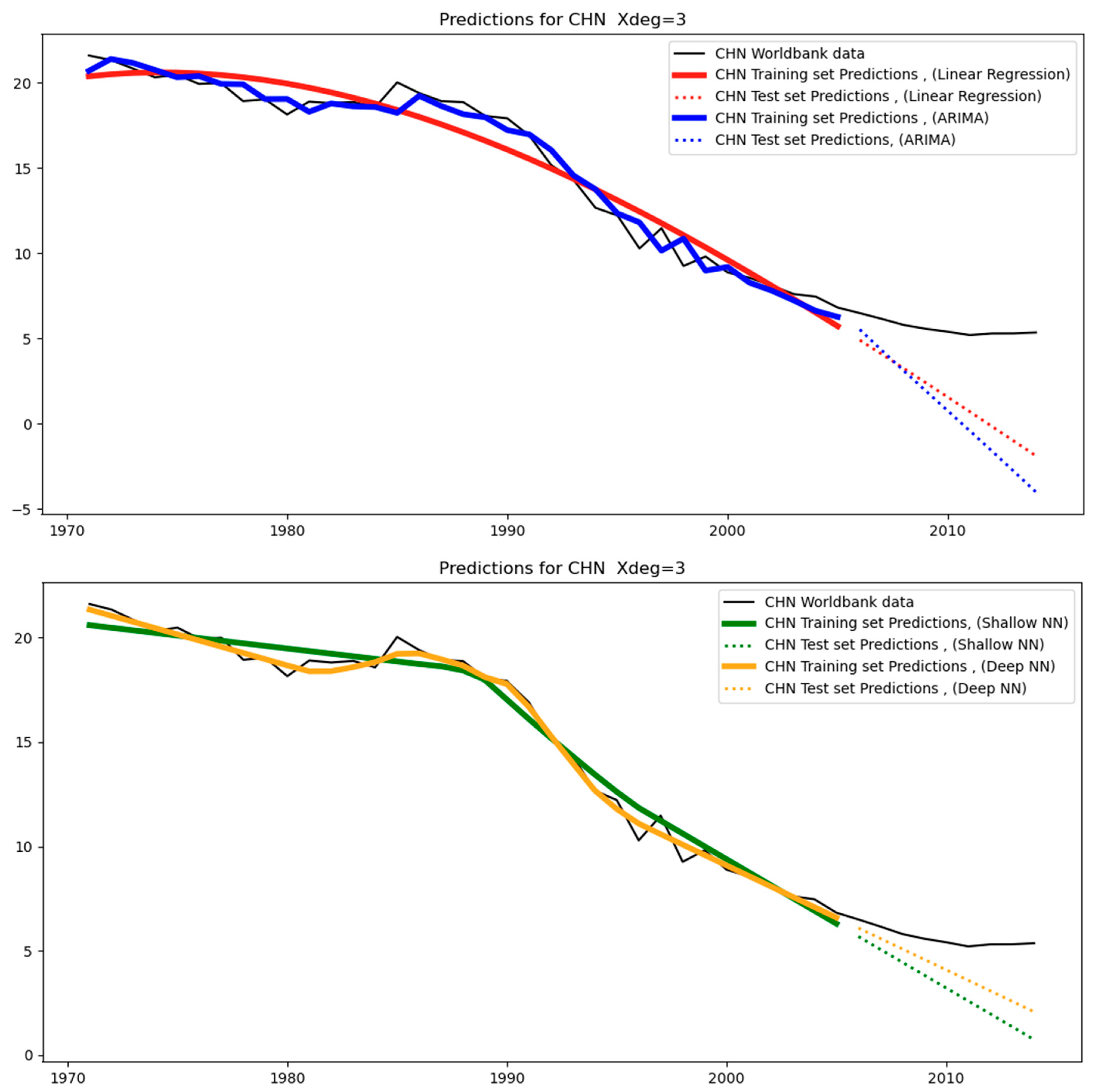
With regards to China, the original data (see Figure 3) displays a clear change of trend immediately after 2005, at the end of the training set, thereby resulting in the highest test-MAPE (see Table 4) over all other regions of the group (India, the USA, WLD, and EUU).

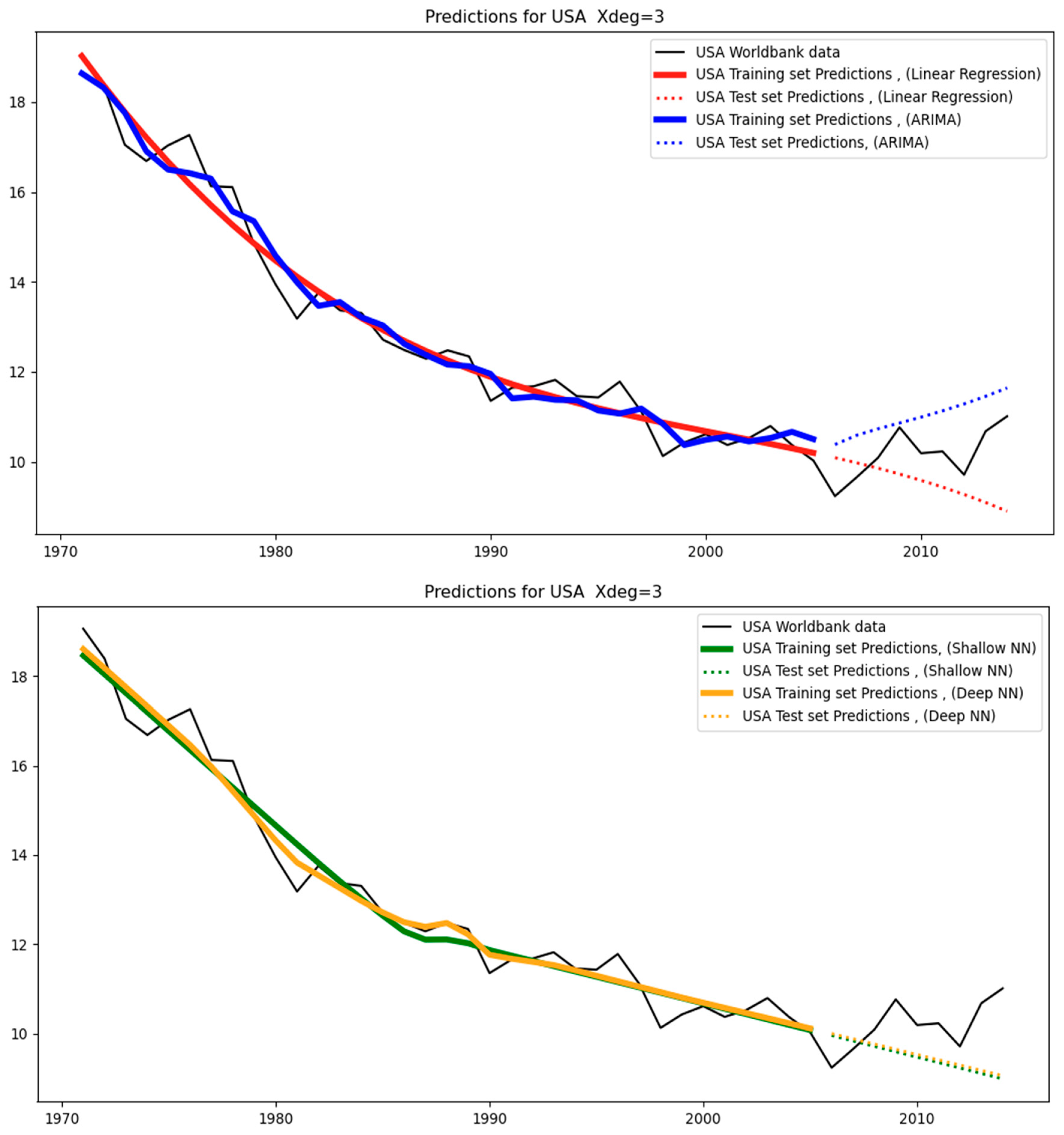
With respect to the USA, WLD, and EUU, they correspond to relatively low test-MAPE because the training and test data (see Figure 3) closely follow a similar trend with a small level of variance. That is, the models are tested on a set that resembles the one to which they were fitted. As a result, for the USA, the test-MAPE is among the smallest (see Table 4). This also applies to WLD, which is the most stable dataset. This is to be expected since it aggregates the data of all the countries, and the resulting low variability helps the models fit the data with high accuracy and the lowest errors across all regions, as can be seen in Table 4. A similar situation applies to EUU, where the data follows a straight line with only a small variance. For this reason, none of these regions leads to overfitting (see Table 6).

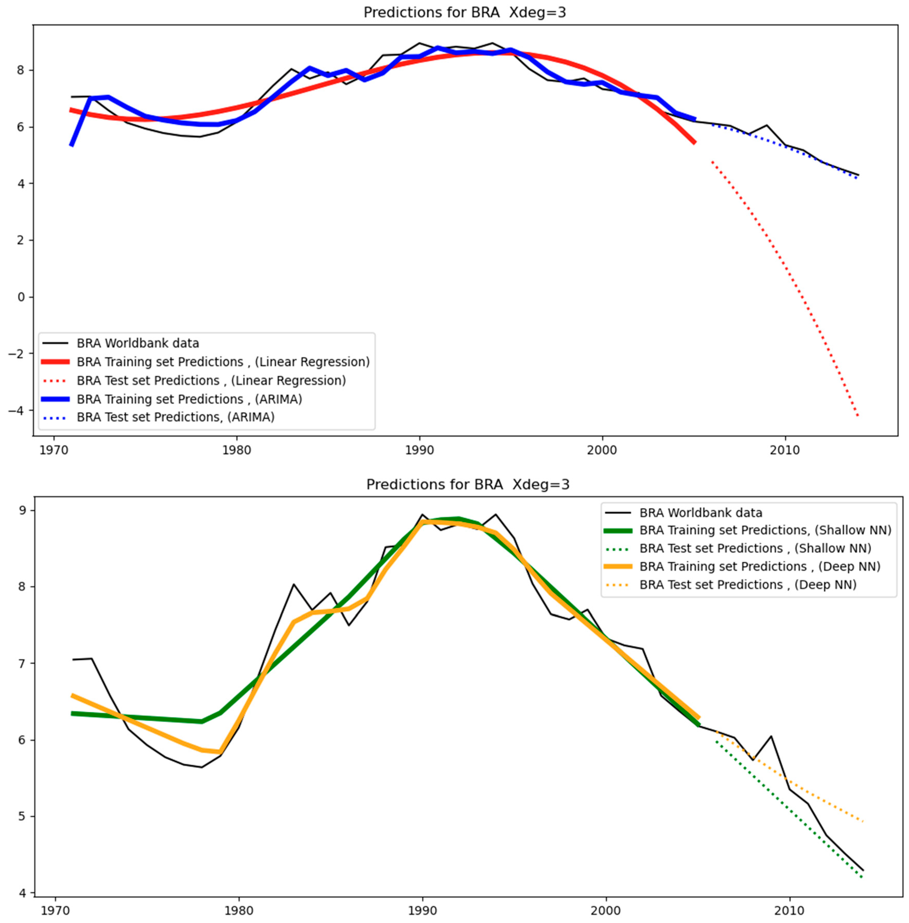
Regarding Brazil (BRA), as can be seen in Table 4, it exhibits the highest test error in linear regression across all regions, which also causes the model to overfit as observed in Table 6. However, there is no overfitting under ARIMA and neural networks, as these models are capable of maintaining the test error close to the training error. This can be witnessed in Figure 10, where we can observe that linear regression is the only model of all and across all regions where the test predictions attain negative values of high magnitude over many years.

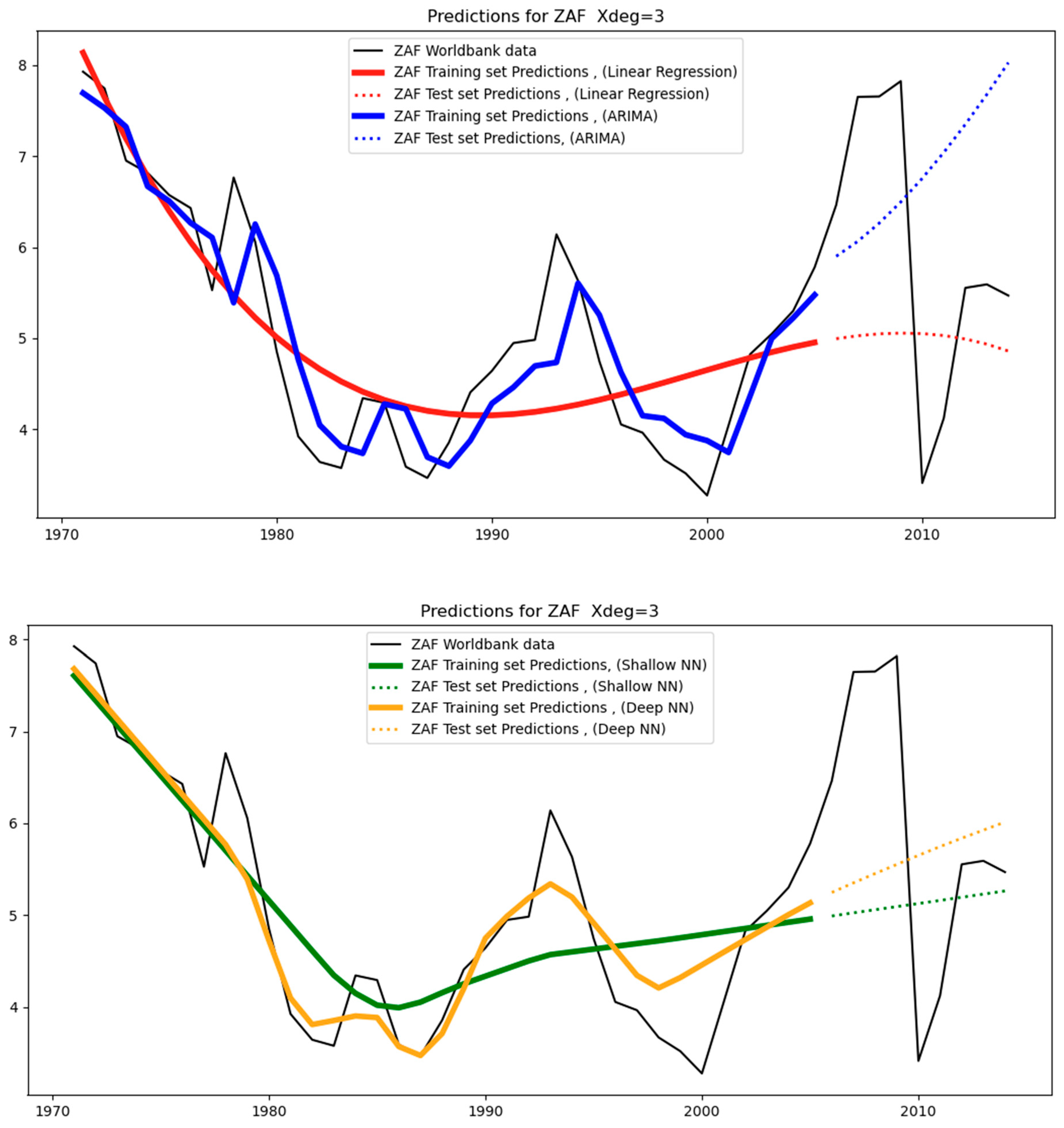
In terms of South Africa, it can be seen in Figure 4 that the dataset is irregular, with the test dataset having a very different pattern from the training set. This renders accuracy in the test predictions particularly challenging. This is why all models for South Africa overfit, as can be seen in Table 6. The training set is much smaller than the test set (see Table 3 and Table 4). Figure 11 illustrates the difficult fitting process for both the training and test sets.

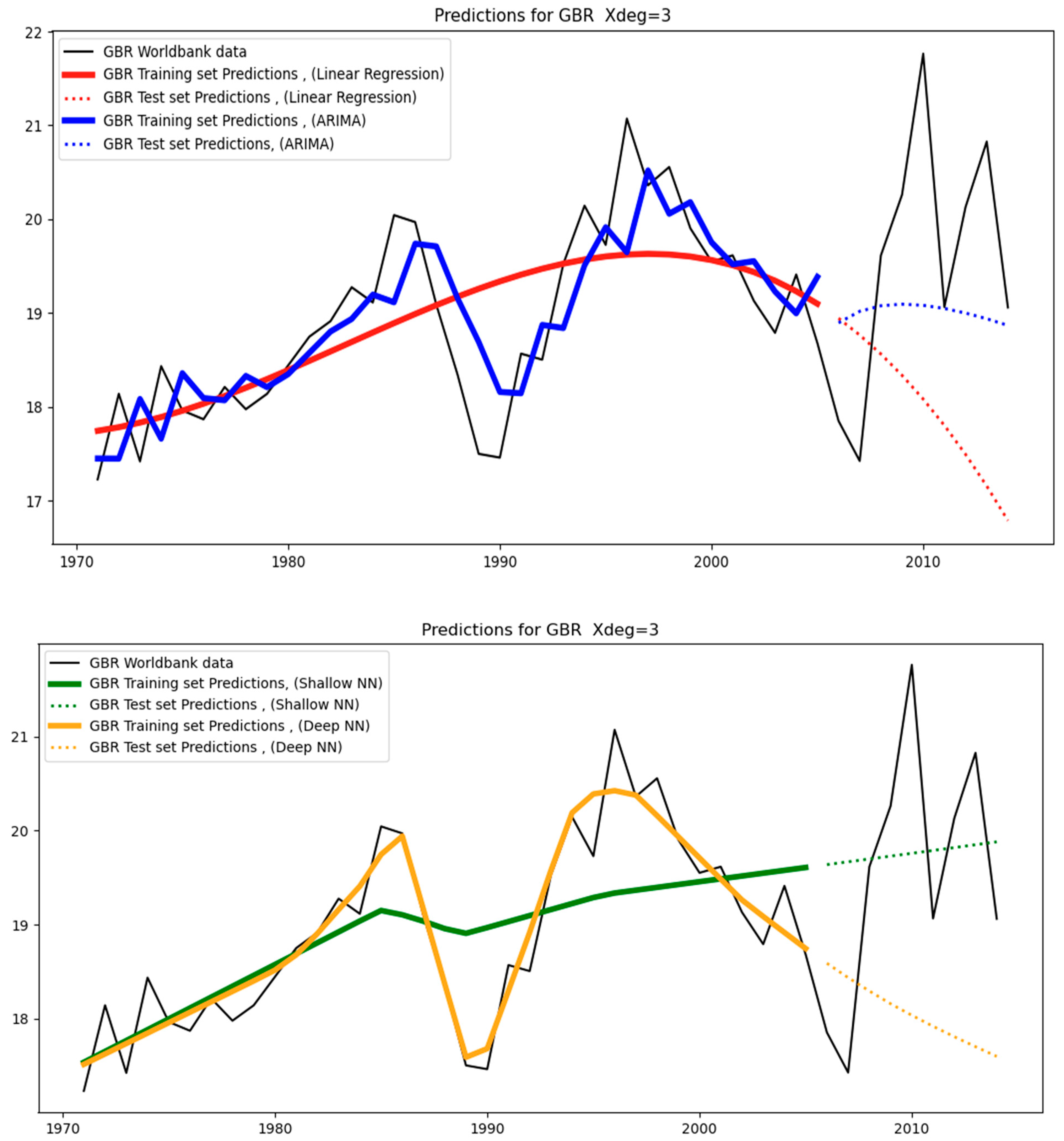
Regarding GBR, despite the high variance (see Figure 4), the test set follows a rather similar trend as the training set, resulting in low errors across the models (see Figure 12 and Table 4).

Table 5 shows that there is significant variation in overfitting per machine learning algorithm.

Table 7. Standard deviation of the difference between the mean average percentage error on the test set and on the training set, under a polynomial degree of three.

	Linear Regression	ARIMA	Shallow NN	Deep NN
Standard Deviation	32.8%	28.8%	13.4%	8.4%

below includes the standard deviation corresponding to each of the algorithms for the values in Table 5; the standard deviation is a measure of how dispersed the data are in relation to the mean. We can observe that the deep neural network models perform better on average, as they exhibit the smallest deviation between test-MAPE and training MAPE, which indicates that they are the least sensitive to dataset patterns.

4.5. Sensitivity Analyses on the MAPE of the Test Set

In this subsection, sensitivity analysis is conducted for each model to evaluate the effect of key hyperparameters on the test-MAPE. This underlines the significance of the test-MAPE as an error metric since it serves as a proxy for the forecast error, indicating the performance of the model on the forecasts.

Table 8. Mean absolute percentage error (MAPE) on the test set using linear regression for different degrees of the polynomial (Deg).

Region	Deg	MAPE
BRA	1	55.77%
	2	3.03%
	3	93.01%
	4	93.49%
IND	1	9.24%
	2	10.05%
	3	15.68%
	4	15.76%
CHN	1	13.27%
	2	96.57%
	3	74.74%
	4	74.12%
ZAF	1	37.73%
	2	39.05%
	3	25.48%
	4	25.54%
USA	1	22.25%
	2	8.64%
	3	8.52%
	4	8.63%
GBR	1	5.88%
	2	5.93%
	3	10.53%
	4	10.60%
WLD	1	2.18%
	2	4.44%
	3	3.79%
	4	3.80%
EUU	1	7.51%
	2	4.38%
	3	11.02%
	4	11.03%

below shows the effect that the degree of the polynomial can have on the MAPE of the test set when using linear regression. As a reminder, the degree of the polynomial is a hyperparameter, and its value determines the number of columns in the features matrix. For instance, when it is equal to one, there is just one column in the feature matrix. This means that the model can capture only linear patterns from inside the training set. This is while, with higher degree polynomials, the model can also capture nonlinear patterns. The higher the polynomial degree, the more complex the patterns the model can capture.

Table 9. Mean absolute percentage error (MAPE) on the test set using ARIMA for different values for the autoregressive ARIMA order (AR), and of the degree of the polynomial (Deg).

Region	MAPE	Deg	AR
BRA	55.74%	1	0
	24.26%	1	1
	33.72%	1	2
	3.03%	2	0
	1.83%	2	1
	2.07%	2	2
IND	9.24%	1	0
	9.43%	1	1
	9.32%	1	2
	10.05%	2	0
	10.05%	2	1
	10.03%	2	2
CHN	13.22%	1	0
	13.62%	1	1
	16.11%	1	2
	96.57%	2	0
	88.93%	2	1
	84.01%	2	2
ZAF	37.76%	1	0
	26.59%	1	1
	29.22%	1	2
	39.05%	2	0
	38.51%	2	1
	37.94%	2	2
USA	22.26%	1	0
	18.27%	1	1
	19.03%	1	2
	8.64%	2	0
	8.12%	2	1
	8.44%	2	2
GBR	5.88%	1	0
	4.85%	1	1
	4.96%	1	2
	5.93%	2	0
	5.81%	2	1
	5.90%	2	2
WLD	2.18%	1	0
	2.19%	1	1
	2.20%	1	2
	4.44%	2	0
	4.16%	2	1
	4.25%	2	2
EUU	7.52%	1	0
	7.05%	1	1
	7.29%	1	2
	4.38%	2	0
	4.36%	2	1
	4.35%	2	2

shows the effect of hyperparameters on the test-MAPE using ARIMA. This sensitivity analysis has been conducted using different combinations of ARIMA orders as well as the degree of the polynomial. Typical values for the autoregressive (AR) order are selected, while the difference (I) and moving average (MA) components are kept to zero.

Table 10. Mean absolute percentage error (MAPE) on the test set using shallow neural networks for different values of the degree of the polynomial (Deg), number of neurons per hidden layer (Un), and number of epochs (No).

Region	MAPE	Deg	Un	No
BRA	33.2%	1	50	50
	15.1%	1	50	100
	25.6%	1	100	50
	6.9%	1	100	100
	26.9%	2	50	50
	13.2%	2	50	100
	22.1%	2	100	50
	5.1%	2	100	100
IND	17.4%	1	50	50
	18.6%	1	50	100
	18.3%	1	100	50
	17.2%	1	100	100
	15.0%	2	50	50
	13.3%	2	50	100
	17.4%	2	100	50
	15.9%	2	100	100
CHN	14.8%	1	50	50
	32.7%	1	50	100
	33.1%	1	100	50
	40.8%	1	100	100
	37.5%	2	50	50
	38.8%	2	50	100
	38.9%	2	100	50
	36.1%	2	100	100
ZAF	28.5%	1	50	50
	25.1%	1	50	100
	26.9%	1	100	50
	25.1%	1	100	100
	27.2%	2	50	50
	24.5%	2	50	100
	25.9%	2	100	50
	23.3%	2	100	100
USA	7.4%	1	50	50
	5.4%	1	50	100
	7.6%	1	100	50
	6.1%	1	100	100
	8.1%	2	50	50
	6.7%	2	50	100
	7.1%	2	100	50
	7.5%	2	100	100
GBR	5.5%	1	50	50
	5.5%	1	50	100
	5.6%	1	100	50
	5.6%	1	100	100
	5.6%	2	50	50
	5.5%	2	50	100
	5.5%	2	100	50
	5.5%	2	100	100
WLD	9.0%	1	50	50
	5.2%	1	50	100
	6.1%	1	100	50
	4.0%	1	100	100
	3.2%	2	50	50
	4.9%	2	50	100
	4.7%	2	100	50
	3.2%	2	100	100
EUU	5.4%	1	50	50
	4.5%	1	50	100
	5.3%	1	100	50
	4.7%	1	100	100
	5.7%	2	50	50
	5.4%	2	50	100
	5.7%	2	100	50
	4.9%	2	100	100

shows the effect of hyperparameters on the test-MAPE using shallow neural networks. Specifically, the hyperparameters include the polynomial degree (Deg), the number of neurons per hidden layer (Un), and the number of epochs (No).

Table 11. Mean absolute percentage error (MAPE) on the test set using deep neural networks for different values of the degree of the polynomial (Deg), number of neurons per hidden layer (Un), and number of epochs (No).

Region	MAPE	Deg	Un	No
BRA	7.0%	1	50	50
	9.0%	1	50	100
	5.5%	1	100	50
	6.1%	1	100	100
	4.2%	2	50	50
	4.1%	2	50	100
	6.7%	2	100	50
	5.5%	2	100	100
IND	13.3%	1	50	50
	13.5%	1	50	100
	11.2%	1	100	50
	13.3%	1	100	100
	12.9%	2	50	50
	12.4%	2	50	100
	10.6%	2	100	50
	13.1%	2	100	100
CHN	34.4%	1	50	50
	16.0%	1	50	100
	29.6%	1	100	50
	25.7%	1	100	100
	28.7%	2	50	50
	28.9%	2	50	100
	30.3%	2	100	50
	25.2%	2	100	100
ZAF	25.7%	1	50	50
	23.3%	1	50	100
	26.0%	1	100	50
	31.6%	1	100	100
	26.7%	2	50	50
	24.4%	2	50	100
	25.8%	2	100	50
	27.4%	2	100	100
USA	8.7%	1	50	50
	8.5%	1	50	100
	8.5%	1	100	50
	8.6%	1	100	100
	8.6%	2	50	50
	8.2%	2	50	100
	9.0%	2	100	50
	8.8%	2	100	100
GBR	5.5%	1	50	50
	8.4%	1	50	100
	6.1%	1	100	50
	9.5%	1	100	100
	5.5%	2	50	50
	7.9%	2	50	100
	6.3%	2	100	50
	9.3%	2	100	100
WLD	4.2%	1	50	50
	4.2%	1	50	100
	5.3%	1	100	50
	4.3%	1	100	100
	3.5%	2	50	50
	4.1%	2	50	100
	5.5%	2	100	50
	4.7%	2	100	100
EUU	5.1%	1	50	50
	4.4%	1	50	100
	4.8%	1	100	50
	4.5%	1	100	100
	4.7%	2	50	50
	4.4%	2	50	100
	4.8%	2	100	50
	4.5%	2	100	100

shows the effect of hyperparameters on the test-MAPE using deep neural networks. The hyperparameters selected include the degree of the polynomial (Deg), the number of neurons per hidden layer (Un), and the number of epochs (No).

The average value of the test-MAPE across Table 8, Table 9, Table 10 and Table 11, along with the standard deviation, respectively, is shown in

Table 12. Average value and standard deviation for the mean average percentage error on the test set corresponding to the sensitivity analysis.

Test-MAPE	Linear Regression (Table 8)	ARIMA (Table 9)	Shallow NN (Table 10)	Deep NN (Table 11)
Average value	25.36%	18.18%	14.73%	12.16%
Standard Deviation	29.41%	22.48%	11.28%	9.14%

below.

The following subsection discusses the results of the sensitivity analysis.

4.6. Discussion on the Sensitivity Analysis

The aforementioned sensitivity analysis is conducted with the sole purpose of gaining more insights into how the test-set MAPE is affected by the values of different hyperparameters. In addition, we obtain significant insights into the models themselves through Table 12. This table shows that deep learning is a more stable modeling approach overall, given the smallest standard deviation across all models. In addition, this approach achieves the highest accuracy on the test predictions given that the average test error is the smallest. These observations, coupled with those in Table 7, underline the superior performance of deep learning in generating forecasts for this case study.

Regarding Table 8, which corresponds to linear regression, it can be stated that a polynomial degree equal to one (i.e., linear fitting) is the best option when the data are a straight line; this applies to IND, CHN, and WLD, where the data approximates a straight line as can be seen in Figure 3. Higher degrees trigger an increase in the test errors, caused by overfitting (for example, see Table 6, which is for a third-degree polynomial); overfitting is caused because the data are too simple (almost linear) for complicated models (i.e., models of high polynomial degrees). Regarding GBR, the general trend is flat (a straight line), as can be seen in Figure 4, which explains why a first-degree polynomial yields the smallest test error in Table 8. On the other hand, degree = 2 is optimal when the data have a single peak, such as when it is a parabola (concave shape) as in the case of Brazil (BRA). For EUU, the case is marginal, and this is why 1st and 2nd degrees yield relatively small tests—MAPE. With regards to the USA, the general trend of the data includes parabolic and nonlinear elements, and degrees greater than two yield optimal values for the MAPE. Furthermore, a degree = 3 is optimal for more complex shapes, such as ZAF.

Regarding Table 9, which corresponds to ARIMA, it can be observed that for linear datasets such as WLD, changing the degree does not have a significant effect. This also applies to IND and GBR, where the data generally follow a straight line, as can be seen in Figure 3 and Figure 4; note that GBR is quite irregular but still retains a flat trend. ARIMA is capable of yielding accurate test predictions in these cases, irrespective of the polynomial degree. On the other hand, for Brazil (BRA), the EUU, and the United States (USA), the second degree reduces the errors because it is more suitable given the presence of nonlinear parts in the datasets. As far as CHN is concerned, the data shows a sudden change in trend immediately after the test set has started. As a result, the error in all the tests is relatively high, but it is smaller under degree = 1 due to the relatively straight shape of the test set. Regarding South Africa (ZAF), the data are very irregular, resulting in relatively high errors regardless of the degree of the polynomial. This indicates that the ARIMA model is not the optimal option for this dataset. In Table 9, we can see that the AR order does not meaningfully change the test error produced. For cases of linear trends in the original data, such as for India (IND), WLD, and EUU, the AR order does not have any effect, while in other cases the effect is relatively small.

Regarding Table 10, which corresponds to shallow neural networks, we can observe the effect of three hyperparameters (namely, the degree of the polynomial, the number of neurons per hidden layer, and the number of epochs) on the test errors. Regarding Brazil (BRA), we observe that increasing the degree to two reduces the error in all situations. This is because the data for Brazil is more complex than a straight line. Therefore, the added complexity (degree = 2) is required. Additionally, increasing the number of neurons (Un) to 100 and the number of epochs (No) to 100 reduces the error in all the situations since the data are more complex than a straight line and the added complexity is required to learn these patterns. In terms of India (IND), there is not much difference between the cases of degree = 1 and 2, given that the data have a linear trend. Regarding China, increasing the degree increases the error because of the sudden change in the trend immediately after the test set has started, resulting in high test-MAPE in all cases. Similarly, the dataset for ZAF is very irregular, resulting in relatively high error under all situations. In terms of the USA, we observe that the errors are relatively small, and this is because the data are slightly parabolic with flat elements. Regarding GBR, the data are quite irregular, but the general trend is flat, resulting in the errors being almost equal to each other. In terms of WLD, the data are close to a straight line, and even with simple models, the resulting errors are small, minimizing the effect of the number of neurons and epochs. Regarding EUU, the data are quite straight with little variance. In this case, both degrees yield relatively small errors.

Regarding Table 11, which corresponds to deep neural networks (deep learning), we can observe the effect of three hyperparameters (namely, the degree of the polynomial, the number of neurons per hidden layer, and the number of epochs) on the test errors. As with the case of shallow neural networks, the effect of the latter two hyperparameters is not significant when keeping the same value for the degree of the polynomial. Regarding Brazil (BRA), it can be seen that the error reduces as the degree increases, which is due to the fact that the data are more complex than a straight line, thereby making the complexity of the second degree necessary for error reduction. Regarding India (IND) and the USA, there is no significant difference given that the data are quite straight with some noise. Similarly, for GBR, the data are irregular but the general trend is flat, and therefore the hyperparameters do not have a notable effect. In terms of China (CHN), since the data have a sudden change in trend immediately after the start of the test set, the resulting error is relatively large. Regarding South Africa (ZAF), since the data are irregular, the resulting errors are relatively high in all cases. Regarding WLD, the data are close to a straight line, and even with simple models, small errors can be achieved. Finally, in terms of EUU, the errors are kept relatively small, given that the data are relatively straightforward.

4.7. The Naïve-Model Benchmark Test

In this subsection, we will conduct the naïve—model benchmark test, which involves comparing the test-MAPE that has been obtained against the test-MAPE of a simplistic/naïve model. This naïve model serves as the benchmark for deciding whether the test-MAPE results obtained are high and therefore not acceptable. That is, the models that have a high test-MAPE are disqualified from generating forecasts since, as mentioned, the test-MAPE is a proxy for the forecasting error, i.e., a model that has a high test-MAPE is likely to have a high forecasting error as well.

Table 13. Predictions of the naïve model. When compared with Table 1, it can be seen that the data have been shifted one row below, i.e., the values for 1971 in Table 1 are now placed in row 2.

Year	BRA	IND	CHN	ZAF	USA	GBR	WLD	EUU
1971	NaN	NaN	NaN	NaN	NaN	NaN	NaN	NaN
1972	7.04	15.08	21.59	7.92	19.06	17.23	18.61	21.95
1973	7.05	14.03	21.32	7.74	18.39	18.14	18.43	22.12
…	…	…	…	…	…	…	…	…
2012	5.16	6.17	5.21	4.12	10.23	19.07	8.81	15.68
2013	4.75	5.70	5.30	5.55	9.71	20.13	8.64	16.34
2014	4.51	5.70	5.30	5.59	10.68	20.82	8.80	17.06

shows the predictions obtained with the naïve model. These are produced by simply shifting the original data one row below. In other words, the model predicts that the next value of the time series will be the same as the current value, i.e., it carries forward the previous value. This is the most common benchmark used in time series forecasting.

Table 14. The mean average percentage error (MAPE) on the test set, per region, using the naïve model.

Region	Naïve Model
IND	4.04%
CHN	3.39%
USA	5.22%
WLD	2.90%
EUU	6.77%
BRA	5.40%
ZAF	22.60%
GBR	6.71%

shows the test-MAPE obtained using the naïve model. These values serve the purpose of the benchmark for the values shown in Table 4, i.e., the test-MAPE obtained using linear regression, ARIMA, shallow neural networks, and deep neural networks.

Table 15. Models that have failed the naïve model benchmark test, i.e., models whose test-MAPE is higher than that shown in Table 14.

Region	Model
IND	Linear Regression
IND	ARIMA
IND	Shallow NN
IND	Deep NN
CHN	Linear Regression
CHN	ARIMA
CHN	Shallow NN
CHN	Deep NN
USA	Linear Regression
USA	ARIMA
USA	Shallow NN
USA	Deep NN
WLD	Linear Regression
WLD	ARIMA
WLD	Deep NN
EUU	Linear Regression
BRA	Linear Regression
BRA	Deep NN
ZAF	Linear Regression
ZAF	ARIMA
ZAF	Shallow NN
ZAF	Deep NN
GBR	Linear Regression
GBR	Deep NN

shows the models that have yielded test-MAPE values (as in Table 4) that are higher than the ones shown in Table 14 and are therefore considered to have unacceptably high test errors and, by extension forecasting errors. The idea is that if the test-MAPE obtained using the simplistic/naïve model is smaller than the test-MAPE obtained using the complex models (linear regression, ARIMA, and neural networks) then the test-MAPE of the latter is considered unacceptably high. This means that these models are not to be used for producing forecasts. For example, the test-MAPE for the linear regression model applied to the IND test is 15.68% (see Table 4), i.e., higher than 4.04%, which is the test-MAPE obtained using the naïve model for India (see Table 14), therefore the former cannot be used for forecasts. Note that the naïve model cannot be used for forecasts either; it is only used for this analysis.

4.8. Forecasts

Figure 13, Figure 14, Figure 15, Figure 16, Figure 17, Figure 18, Figure 19 and Figure 20 below show the forecasts obtained per region and model. The hyperparameters that have been used are the ones used for generating the predictions as described in Section 4.1, for example, a third-degree polynomial. Then, Section 4 discusses the results.

5. Analysis of the Results

In the previous section, the models were trained and produced forecasts. However, it is important to filter the models in terms of which can eventually be deemed the most trustworthy in terms of their forecasts. As mentioned, the models that can be used for producing forecasts are the ones that have passed the overfitting test and the naïve-benchmark test. Both tests need to have been passed for the models to be considered reliable for forecasts.

Table 16. Performance of models per test. F and S stand for failed and succeeded, respectively. The models that pass both tests are in bold.

Region	Model	Overfitting Test	Naïve-Benchmark Test	Result
IND	Linear Regression	F	F	F
IND	ARIMA	S	F	F
IND	Shallow NN	F	F	F
IND	Deep NN	F	F	F
CHN	Linear Regression	F	F	F
CHN	ARIMA	F	F	F
CHN	Shallow NN	F	F	F
CHN	Deep NN	F	F	F
USA	Linear Regression	S	F	F
USA	ARIMA	S	F	F
USA	Shallow NN	S	F	F
USA	Deep NN	S	F	F
WLD	Linear Regression	S	F	F
WLD	ARIMA	S	F	F
WLD	Shallow NN	S	S	S
WLD	Deep NN	S	F	F
EUU	Linear Regression	S	F	F
EUU	ARIMA	S	S	S
EUU	Shallow NN	S	S	S
EUU	Deep NN	S	S	S
BRA	Linear Regression	F	F	F
BRA	ARIMA	S	S	S
BRA	Shallow NN	S	S	S
BRA	Deep NN	S	F	F
ZAF	Linear Regression	F	F	F
ZAF	ARIMA	F	F	F
ZAF	Shallow NN	F	F	F
ZAF	Deep NN	F	F	F
GBR	Linear Regression	S	F	F
GBR	ARIMA	S	S	S
GBR	Shallow NN	S	S	S
GBR	Deep NN	S	F	F

below shows whether the models have passed these two tests or not; this analysis is based on Table 6 and Table 14.

According to Table 16, the models that pass both tests, which are shown in bold font, are the following:

-

ARIMA applied to EUU, BRA, and GBR.

-

Shallow Neural Networks applied to WLD, EUU, BRA, and GBR.

-

Deep neural networks applied to EUU.

As a result, all the forecasts shown in Figure 13 (IND) are not accepted. After all, this is obvious from the fact that the forecasts attain negative values, which is clearly unrealistic as CO₂ emissions can never become negative. Additionally, Figure 14 (CHN) is rejected; this is again obvious given the negative forecasts. In addition, Figure 15 (USA) is rejected given that none of the models has passed both tests.

Regarding Figure 16, corresponding to WLD, only the forecast produced using shallow neural networks is accepted. This indicates a linear reduction in CO₂ emissions from buildings all the way to 2050.

In terms of Figure 17, for EUU, the forecasts using ARIMA, shallow and deep neural networks are accepted given that the corresponding models have all passed both tests; the ARIMA forecasts do not seem realistic, but they are still considered.

With respect to Figure 18, for Brazil (BRA), the forecasts using ARIMA and shallow neural networks are accepted. However, if we consider the additional constraint that CO₂ emissions cannot be negative, then the ARIMA forecasts are rejected as they yield negative values.

In terms of Figure 19, for South Africa (ZAF), all forecasts are rejected as the models have failed to pass both tests. Finally, in Figure 20 (GBR), the acceptable forecasts use ARIMA and shallow neural networks.

Notice that this forecasting analysis is based on the assumption that no major unexpected events will occur until the year 2050 compared to the period 1971–2014 covered by the original dataset, in which the models were trained. Such events can include major wars, economic crises, pandemics, etc. If such events occur, then it is advised that new data be fed to the models and the analysis be repeated.

6. Key Points

This study addresses the need for a clearly defined set of steps that will produce a more accurate and reliable forecast. The presented ten-step methodology starts with the selection of the dataset and then, through a series of tests, such as the naïve-benchmark and overfitting tests, arrives at forecasts that are neither overfit nor have high errors. A significant advantage of this methodology is that it is data-independent. This means that it can be applied to any dataset/time series and is not restricted only to CO₂-related time series. In this context, the merits and implications of this study can be summarized as follows:

• It presents a clearly defined set of steps for obtaining forecasts from machine learning models that have successfully passed a set of tests, thereby increasing the likelihood of obtaining forecasts of high accuracy.
• It is dataset-independent, i.e., it can be applied to any time series.
• It is expandable to more algorithms, meaning that it is not only restricted to the algorithms presented in this paper (linear regression, ARIMA, shallow neural networks and deep learning) but can also include more algorithms.

7. Conclusions and Future Work

This work presents for the first time in the literature the application of a machine learning-based methodology for generating forecasts of CO₂ emissions that are specifically related to the buildings sector, across different regions of the world (Brazil, India, China, South Africa, the United States, Great Britain, the world average, and the European Union). Note also that the data used originated from the official database of the World Bank and covered the period 1971–2014.

This methodology consists of ten steps as presented in Figure 1, namely (a) data preprocessing, (b) dataset Split, (c) data Scaling, (d) model fitting, (e) calculation of training-set errors and test errors, (f) overfitting analysis, (g) sensitivity analysis, (h) forecasts and (i) analysis. Note that the selected period for the forecasts stretches up to the year 2050.

The machine learning models that are used include linear regression, ARIMA, shallow neural networks, and deep neural networks (deep learning). These models are first fitted to the training set (years 1971–2005), then applied to the test set (years 2006–2014), and tested for overfitting using a benchmark of 10% for the difference between the test-set errors and the training-set errors; the error metric used is the mean absolute percentage error or MAPE. Those models that have passed the overfitting test successfully also have to pass the naïve-benchmark test. As a result, only the forecasts corresponding to models that have passed both tests and that are also not attaining negative values can be accepted.

Finally, deep learning has demonstrated superior performance over the other algorithms since it has shown less sensitivity to the value of hyperparameters, smaller test errors, and a smaller degree of overfitting on average.

Future work includes the application of additional machine learning methodologies for forecasting the CO₂ emissions from buildings, such as recurrent neural networks. In addition, it is of interest to the authors to focus on optimizing the value of hyperparameters. Methods that can be used for this purpose include heuristics such as backwards induction [42] and uncertainty analysis methods based on the combination of machine learning with reliability theory [43] and artificial neural networks [44]. The authors are also interested in evaluating the effect of external factors, such as the level of technological development and GDP, on the forecasts in these regions.