Frequency Stabilization in an Interconnected Micro-Grid Using Smell Agent Optimization Algorithm-Tuned Classical Controllers Considering Electric Vehicles and Wind Turbines

Abstract

In micro-grids (MGs), renewable energy resources (RESs) supply a major portion of the consumer demand. The intermittent nature of these RESs and the stochastic characteristics of the loads cause a frequency stabilization issue in MGs. Owing to this, in the present manuscript, the authors try to uncover the frequency stabilization/regulation issue (FRI) in a two-area MG system comprising wind turbines (WTs), an aqua-electrolyzer, a fuel cell, a bio-gas plant, a bio-diesel plant, diesel generation (DG), ship DG, electric vehicles and their energy storage devices, flywheels, and batteries in each control area. With these sources, the assessment of the FRI is carried out using different classical controllers, namely, the integral (I), proportional plus I (PI), and PI plus derivative (PID) controllers. The gain values of these I, PI, and PID controllers are tuned using the recently proposed smell agent optimization (SAO) algorithm. The simulation studies reveal the outstanding performance of the later controller compared with the former ones in view of the minimum settling period and peak amplitude deviations (overshoots and undershoots). The SAO algorithm shows superior convergence behavior when tested against particle swarm optimization and the firefly algorithm. The SAO-PID controller effectively performs in continuously changing and increased demand situations. The SAO-PID controller designed in nominal conditions was found to be insensitive to wide deviations in load demands and WT time constants.

1. Introduction

The continuous utilization of fossil-fuel-based energy sources over the past few decades has not only depleted their available levels but also raised environmental concerns about, for example, global warming, air pollution, the greenhouse gas effect, etc. Owing to this, in recent years, renewable energy resources (RESs) have been promoted in place of fossil fuels for the generation of power. A micro-grid (MG) can supply power to remote areas that are difficult to feed from conventional coal-based sources due to geographical conditions. An MG mainly comprises RESs, resulting in cleaner power production and a reduction in power losses. Despite the cleaner energy production using RESs, their intermittent nature and associated uncertainties make the operation of a micro-grid difficult, particularly due to the oscillations in frequency and power that require proper regulation [1]. Storage devices act as the supplement solution for the frequency regulation issue (FRI) in the event of a mismatch between the load demand and generation, including the intermittent nature of RESs [2,3]. A micro-grid comprises various distributed energy resources (DERs) that include RESs such as solar photovoltaic systems and wind turbines, storage devices, and connected loads.

Electric vehicles (EVs) play an important role in the future automotive industry as they facilitate environmentally friendly technology with significant reductions in hazardous greenhouse gas emissions and energy-saving features. Furthermore, EVs can be used for energy storage (ES) in power grids that can exchange power with the grid bi-directionally, i.e., during charging, an EV functions as a consumer in the grid, while during discharging, as a power producer. Hence, EVs play an important role in enhancing the operation of micro-grids. The main challenge in a micro-grid is that it accumulates intermittent RESs whose behavior is unpredictable and creates continuous frequency fluctuations, which needs to be addressed.

A critical literature survey reveals that a considerable amount of research work on addressing micro-grid frequency regulation has been reported [2,3,4,5,6,7,8,9,10,11,12,13,14,15,16,17,18,19,20,21,22,23,24]. Frequency stabilization in isolated micro-grids is addressed in [2,4,5,6,7,8,9,10,11,12,13,24], and that in interconnected environments is explored in [3,14,15,16,17,18,19,20,21,22,23]. The investigation in [4] took wind turbines (WTs), bio-diesel (BD), solar-thermal (ST) plants, fuel cells (FCs), and water heaters (WHs) into consideration. In [5,6,7,8,9], the studies considered photovoltaics (PV), diesel generators (DGs), WTs, FCs, and/or AEs, along with battery and flywheel storage. The investigation in [10] explored the micro-grid stability issue with an ST plant, WTs, DG, an AE, an FC, and battery storage. With electric vehicles (EVs), DG, and WTs, the micro-grid frequency problem is addressed in [11,12]. WTs, DG, and battery storage were studied in [13]. A two-zone MG system interconnected with DG, WTs, an FC, PV, and EVs was studied in [3]. A two-area-based WT, PV, DG, and battery storage MG system was investigated by Lal et al. [14]. Bio-diesel, micro-hydro turbines, and ST plants in an interconnected environment were considered by the authors of [15]. WTs, PV, and DG with a storage system interconnected micro-grid is considered in [16]. Ranjan et al. [17] studied a three-zone interconnected micro-grid with WT, ST, bio-gas, and PV units. Latif et al. [18] applied a strategy to stabilize the dynamics in a two-zone micro-grid with a WT, DG, a heat pump, and a freezer. A two-zone micro-grid with ST, WP, AE, FC, and battery storage units was studied in [19]. A multi-micro-grid with WP, PV, and DG plants is considered in [20]. In [21] and [22], a two-zone micro-grid with DG, WP, and PV plants and a storage system was studied. Bhuyan et al. [23] investigated a two-zone micro-grid system with ST, BD, battery, and super-conducting magnetic storage units.

Energy storage devices play an important role in frequency stabilization in micro-grids. They store the excess power generated in off-peak hours while releasing energy during peak demand hours. Owing to these advantages, the studies in [5,6,7,8,9] utilized both flywheel and battery storage, whereas the authors of [10,13] considered a battery storage system alone.

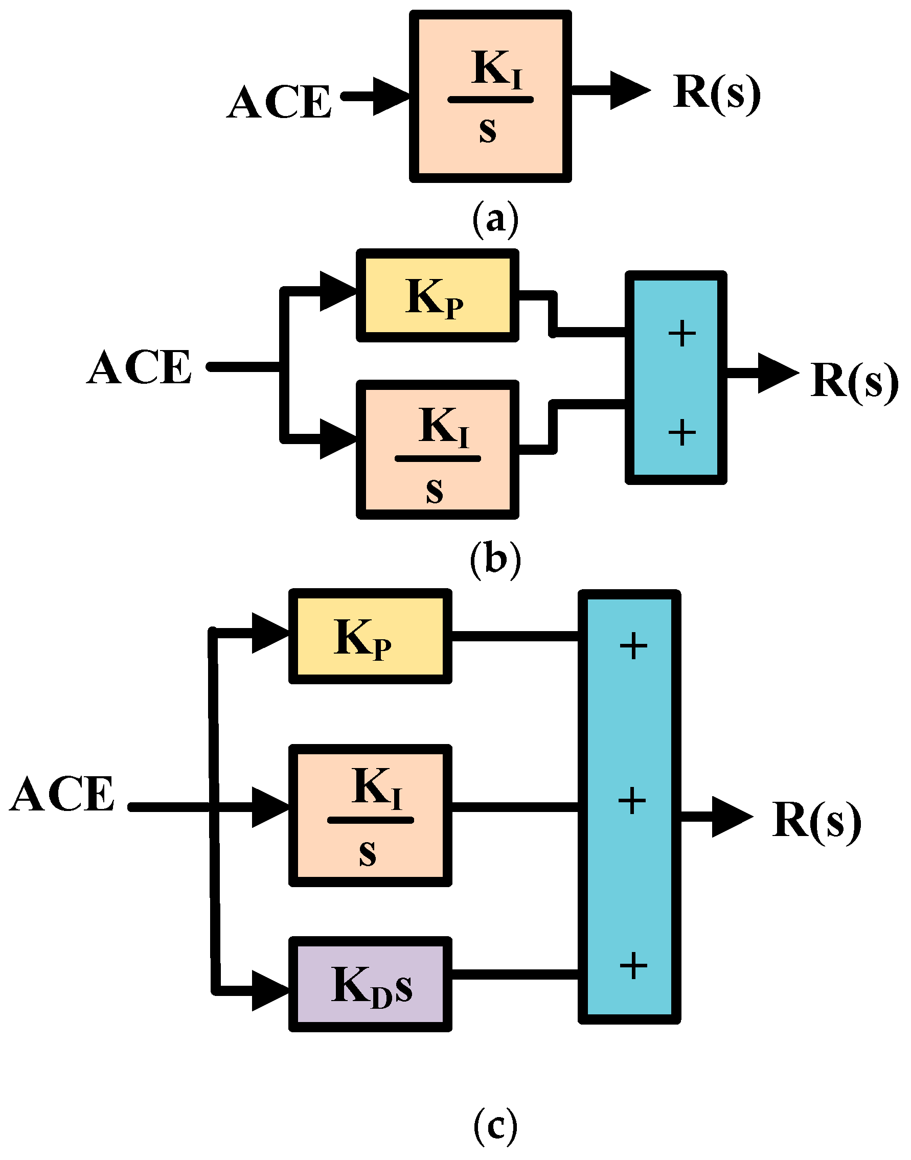
To stabilize fluctuations due to the randomized behavior of RESs and loads, a suitable controller is necessary for a micro-grid system. Owing to this, in the literature, different controllers have been applied to the FRI pertaining to MGs [2,4,5,6,8,10,12,13,14,15,16,17,18,19,21,22,23]. The studies in [5,8,13,16,17,19,21] addressed the FRI using a proportional–integral–derivative (PID) controller. A dual-degree PID (DD-PID or 2DOF-PID) controller was implemented in [10]. The utilization of non-integer controllers, i.e., fractional-order controllers, is observed in [18,22]. A cascade control mechanism with master and slave controllers was applied to solve the FRI in micro-grids by the researchers in [6,15,23]. PI controllers have been applied in investigations [13,24]. Intelligent-based fuzzy logic controllers were used in [12,14,15]. A two-stage controller was also implemented in the investigations carried out in [4]. The PID controller is versatile and popularly used owing to its superior dynamic and robust performance [8]. It is simple in structure, easy in tuning, reliable, requires minimal expertise, and offers a balance between performance and cost [1].

Once the controller is selected, it is expected that the controller adapts itself to varied system conditions, particularly in a micro-grid with intermittent RESs. To achieve the robust and adaptive nature of the controller, its knobs (gains or parameters) should be gained through a global optimization algorithm. In literature, the techniques such as genetic algorithm (GA) [25], particle swarm optimization (PSO)-based robust optimization [26], the firefly algorithm (FA) [8], cuckoo search (CS) methods [13], social spider optimization (SSA) [16], mine blast algorithm (MBA) [17], teaching–learning-based optimization (TLBO) [21], hybrid PSO–gravitational search algorithm [5], etc., have been applied to obtain the optimal knobs of the controller.

By critically analyzing the literature survey, the following research gaps have been identified:

i.

Frequency stabilization for a micro-grid system comprising bio-gas [17] and a ship diesel generator (SDG) [27] is in infancy and needs further investigations.

ii.

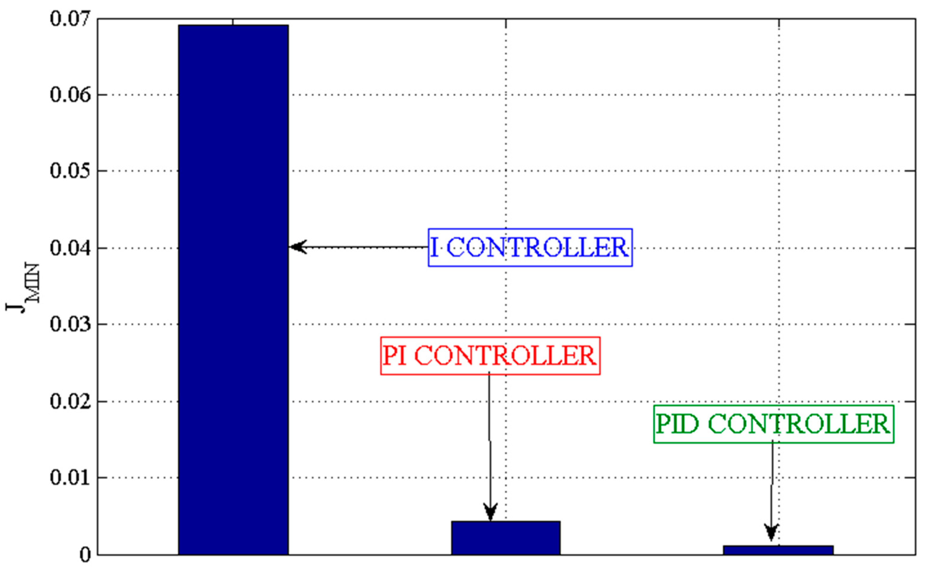
The comparative analysis of classical controllers, namely, the integral (I), proportional plus I (PI), and PI plus derivative (PID) controllers, has not been performed for a micro-grid system with BD, a SDG, WTs, an AE, an FC, DG, EVs, and storage (BES and FES).

iii.

The recently proposed smell agent optimization (SAO) algorithm offers advantages in finding the global optimum for 76% of benchmark functions and the cost-effective design of a hybrid renewable energy system [28]. The SAO algorithm has not been applied for tuning different controller knobs, which guarantees better micro-grid performance.

iv.

The effectiveness of the SAO algorithm has not been tested against particle swarm optimization (PSO) and firefly algorithm (FA) for the stabilization of micro-grid oscillations.

Based on the findings of the research gaps and literature survey, the major contributions of this manuscript are as follows:

i.

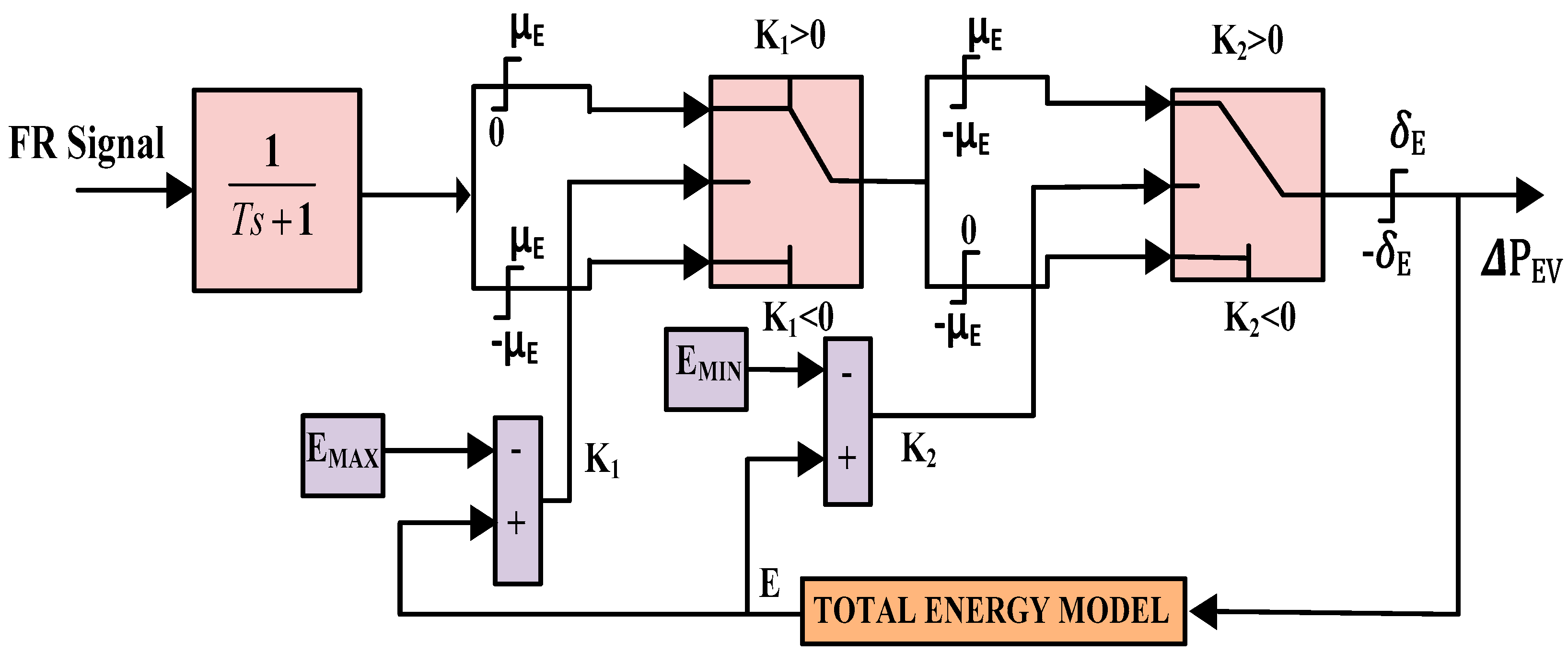
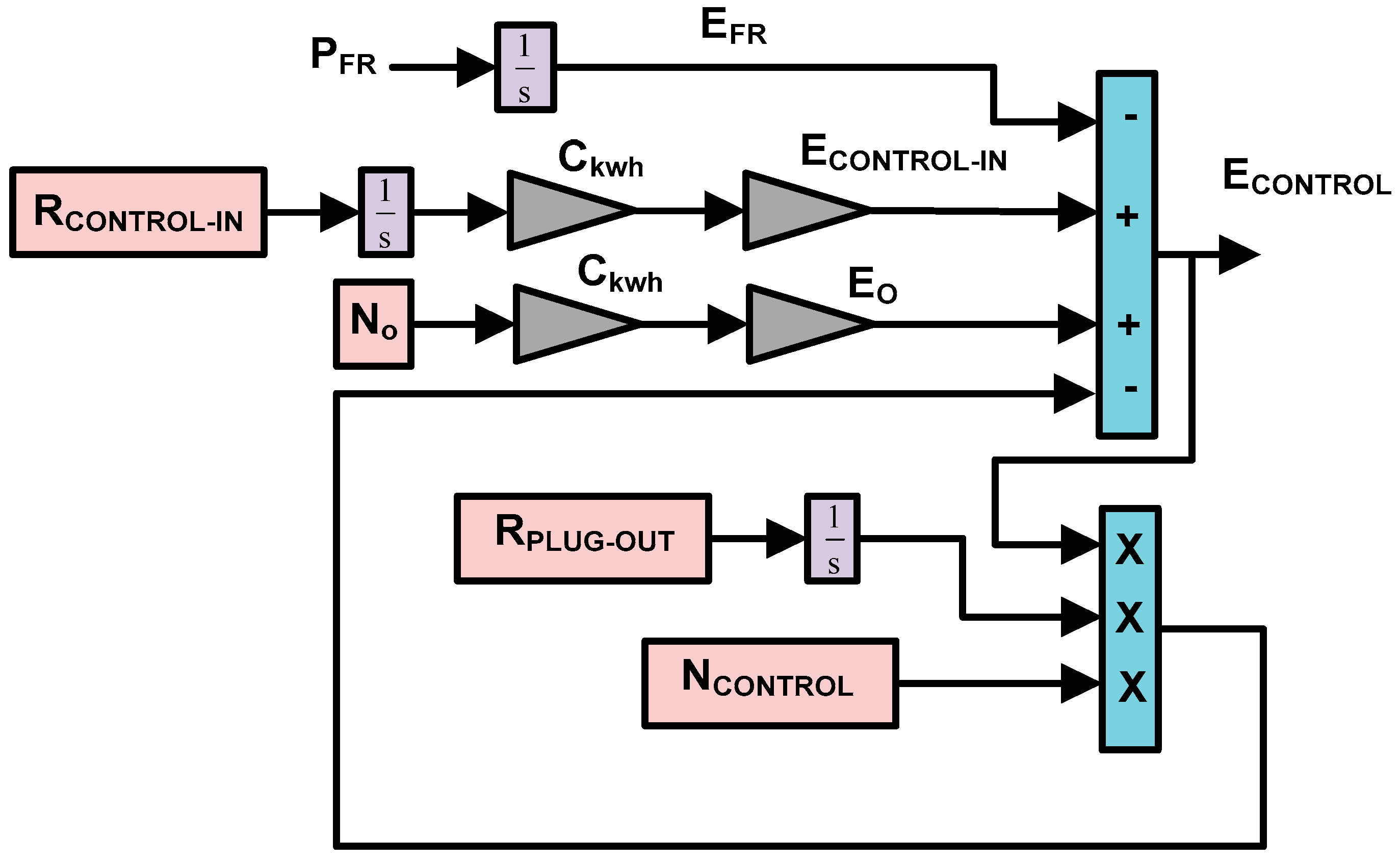
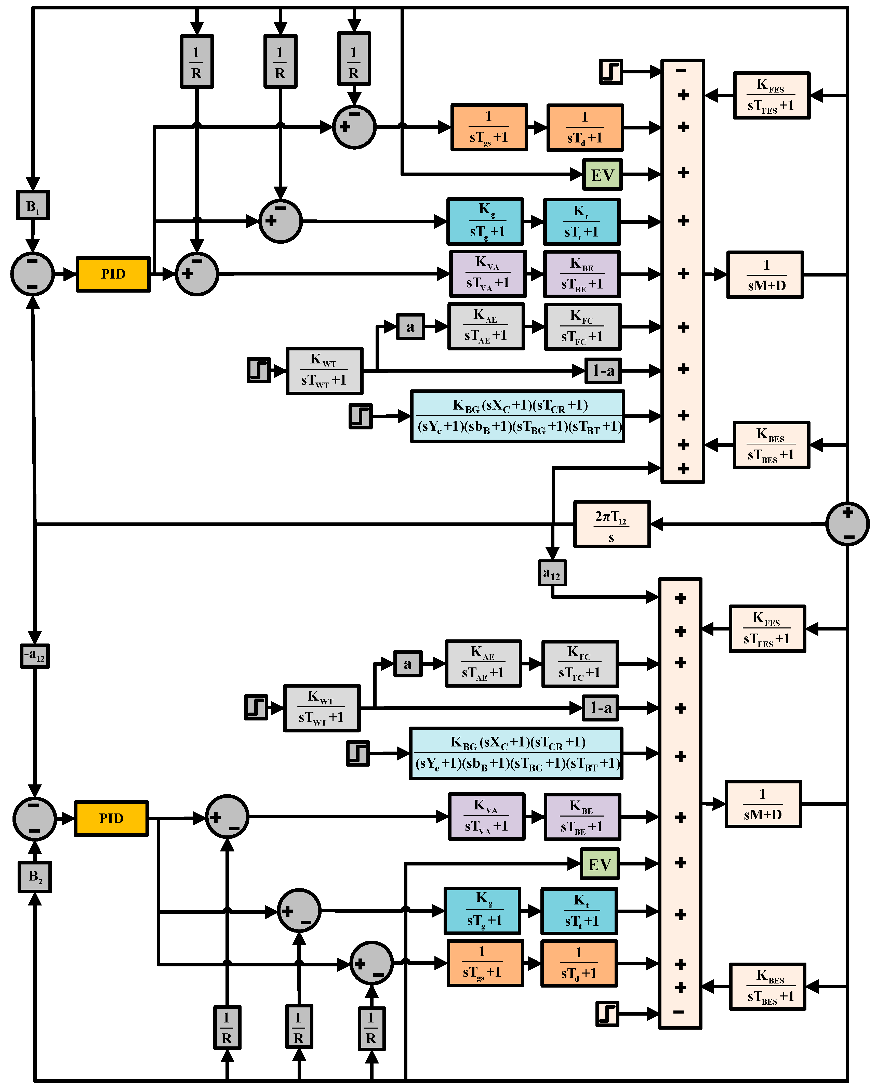
We model the dual-area interconnected small-signal analysis model of a micro-grid system comprising wind turbines (WTs), an aqua-electrolyzer (AE), fuel cell (FC), bio-gas (BG) plant, bio-diesel (BD) plant, diesel generation (DG), ship DG, electric vehicles (EVs) and their energy storage devices, flywheels, and batteries in each control area.

ii.

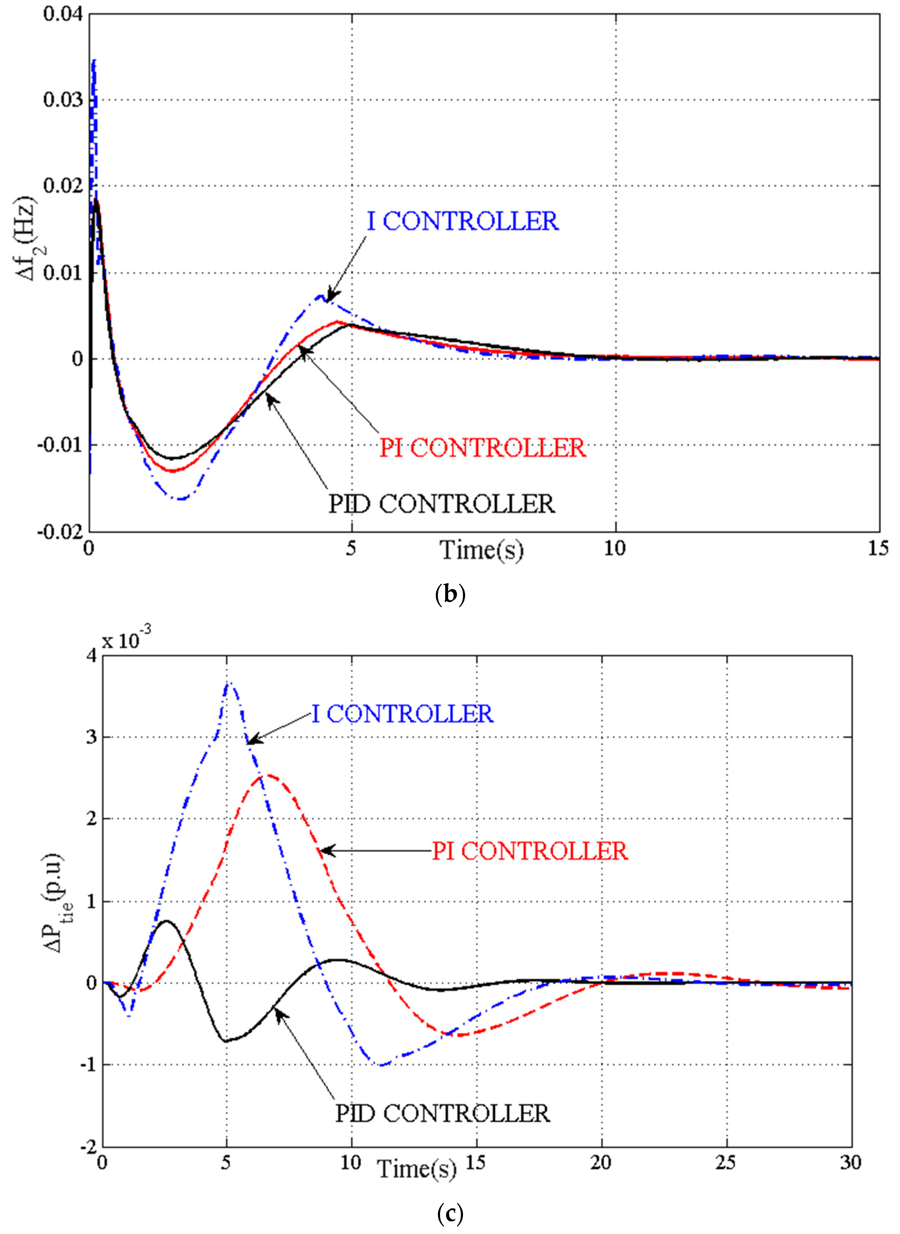
We apply various classical controllers, namely, the integral (I), proportional plus I (PI), and PI plus derivative (PID) controllers, to regulate the frequency of the micro-grid system.

iii.

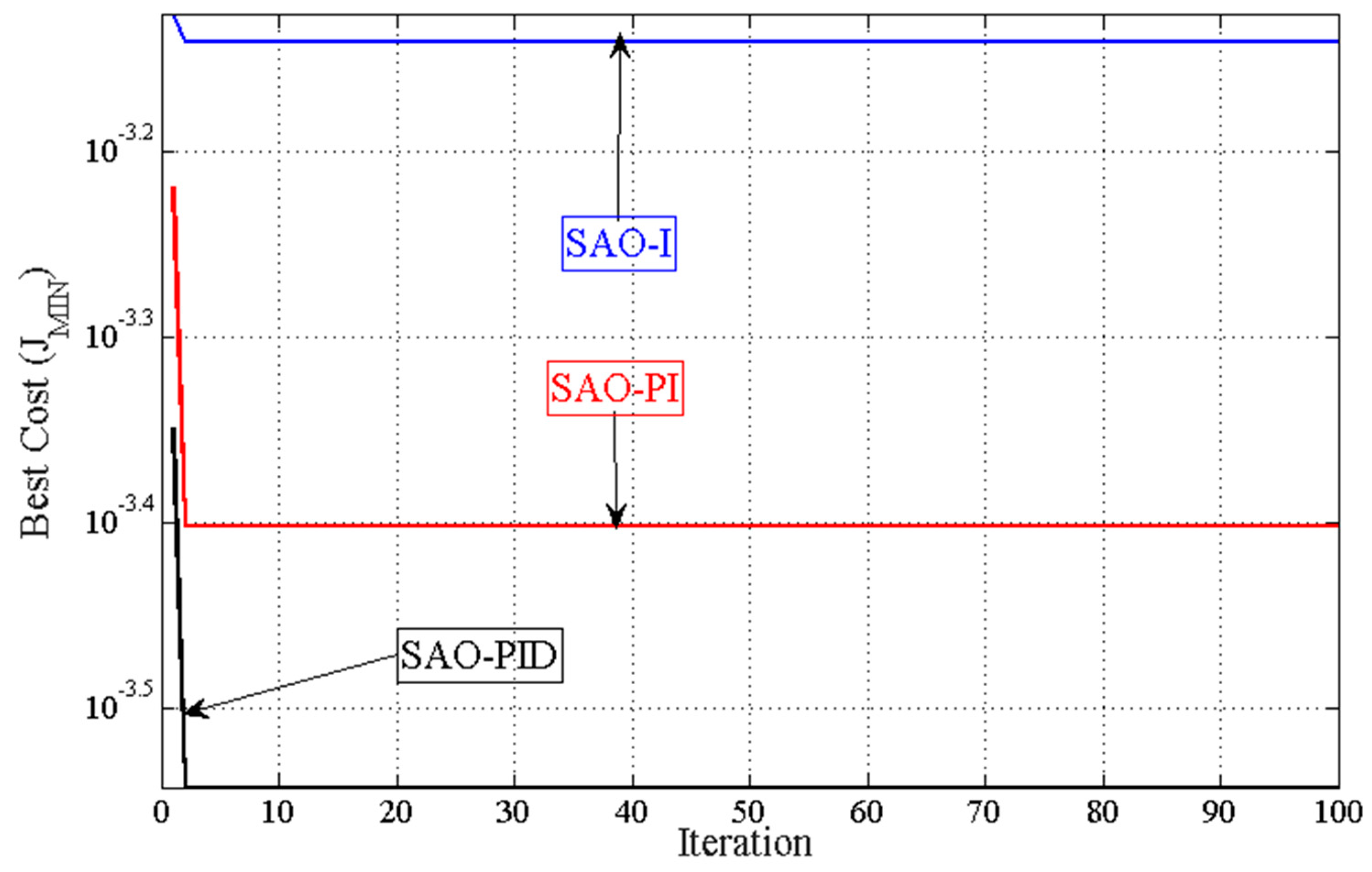
We apply the smell agent optimization (SAO) algorithm for the first time to optimize the above controller parameters to regulate oscillations in the MG system considered in i.

iv.

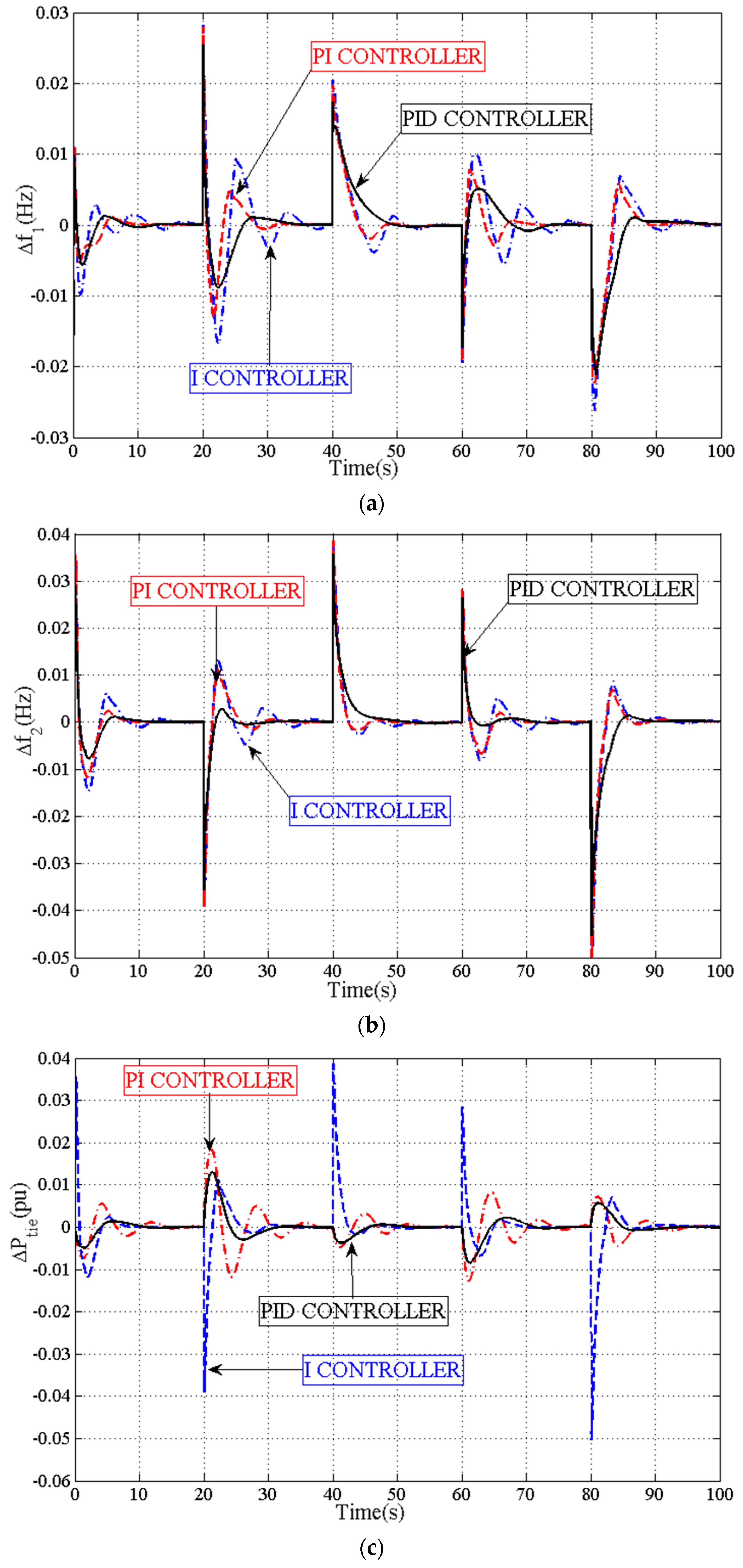
We study the comparative behavior of these classical controllers to decide the best among them.

v.

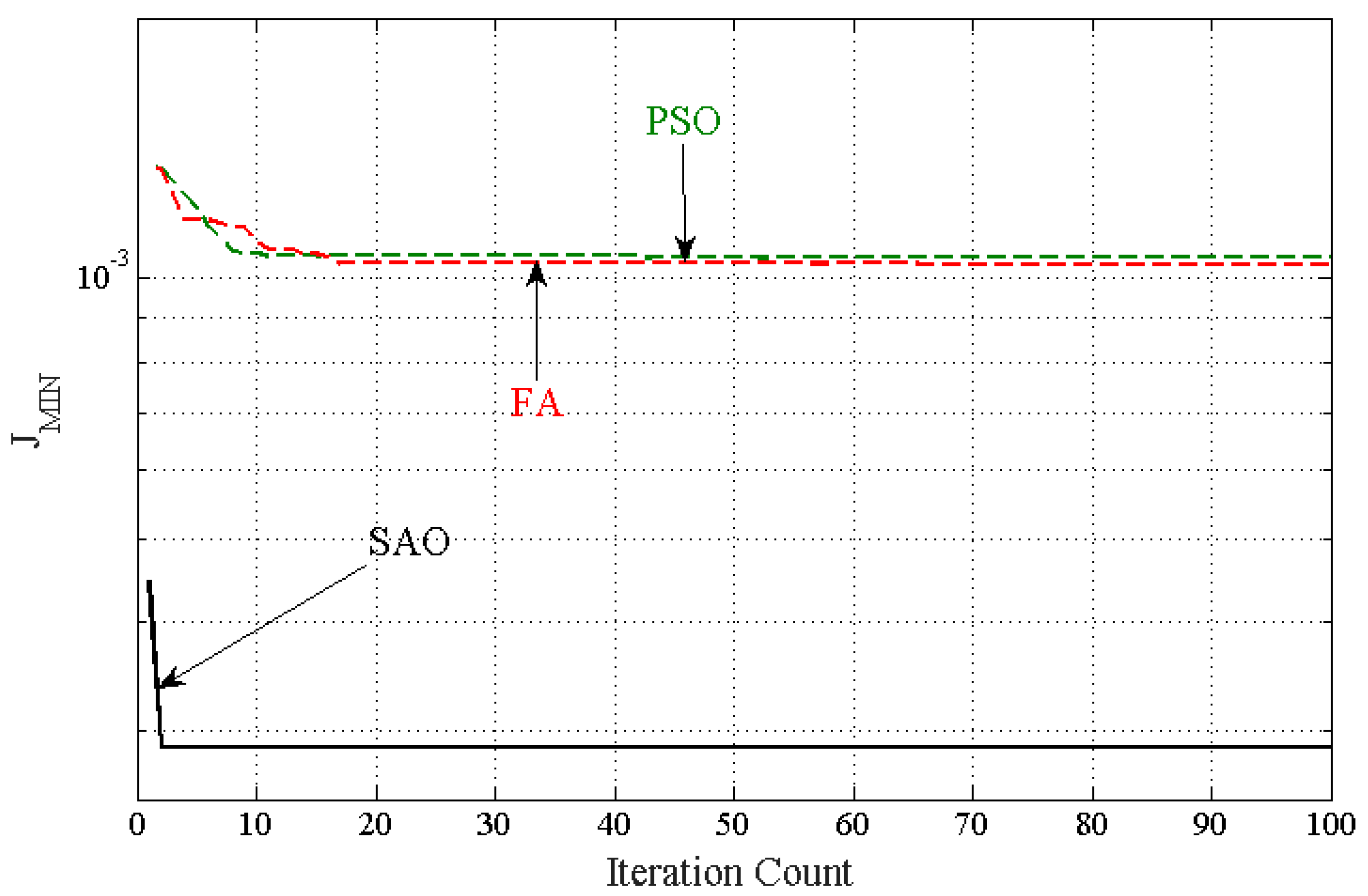
We show the effectiveness of the SAO algorithm compared with the commonly employed particle swarm optimization (PSO) and firefly algorithm (FA).

vi.

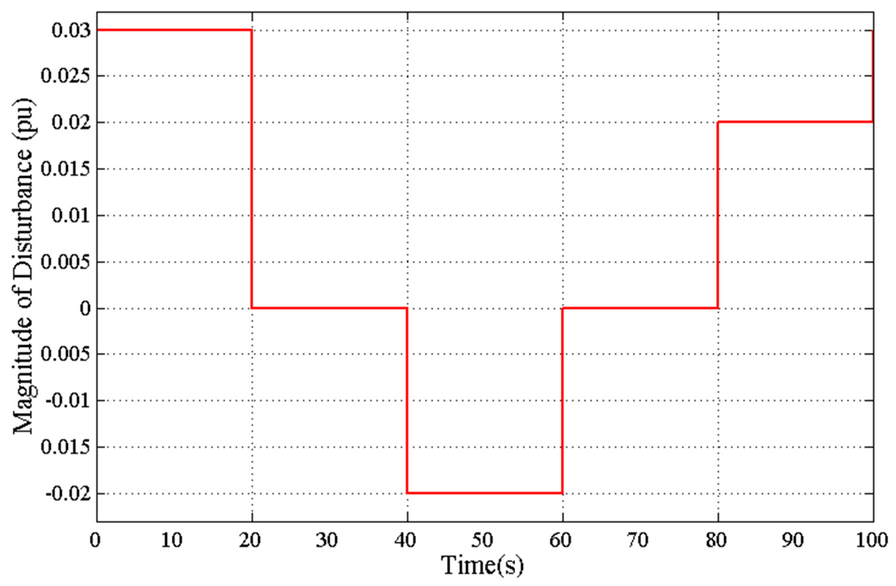
We observe the SAO-tuned PID controller performance compared with the I and PI controllers for randomized load demand patterns.

vii.

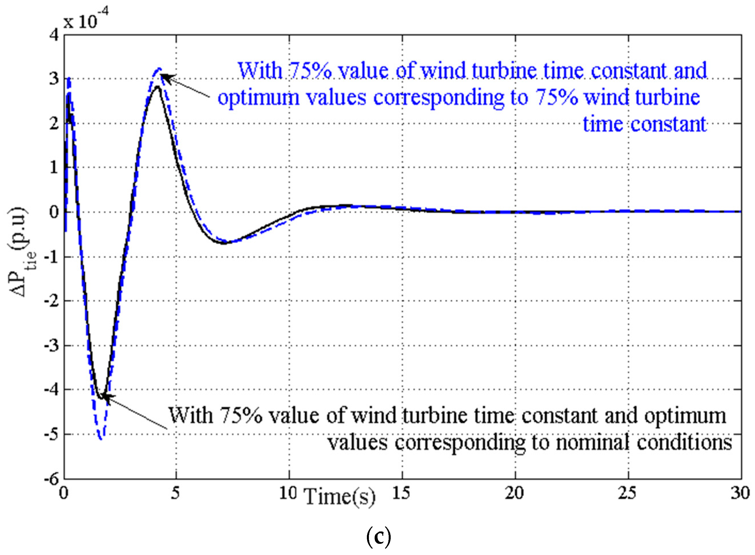
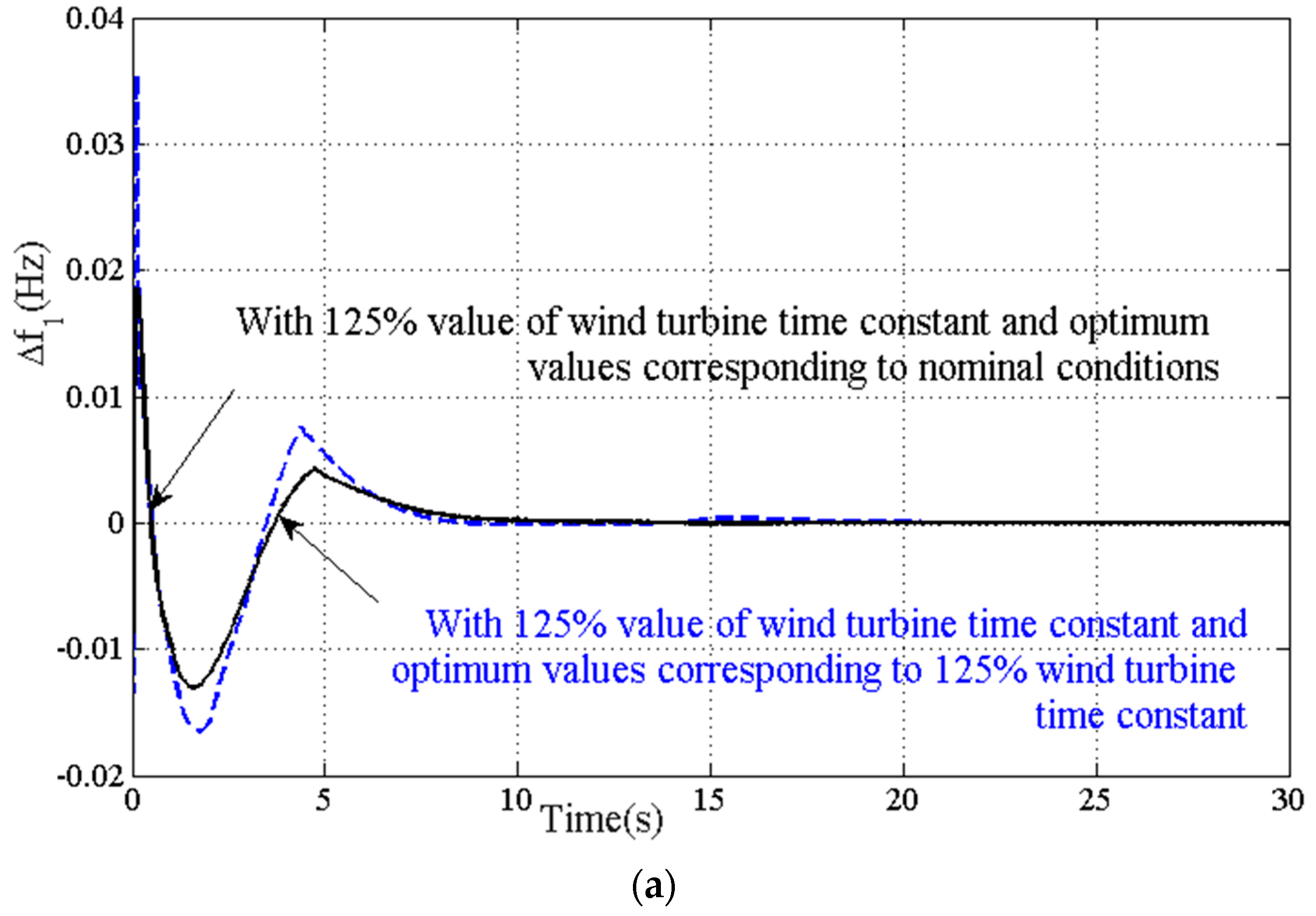
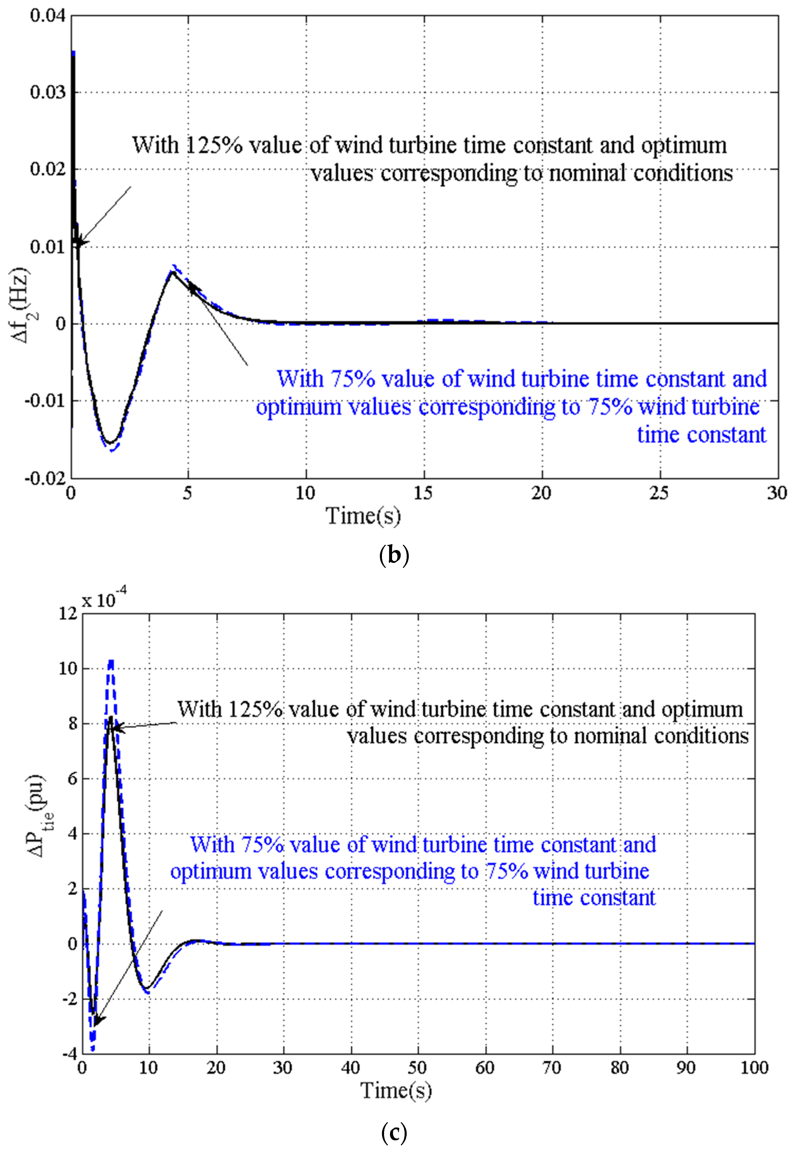
We observe the toughness of the SAO-tuned PID controller parameters with a larger load demand and deviations in the time constant values of WTs.

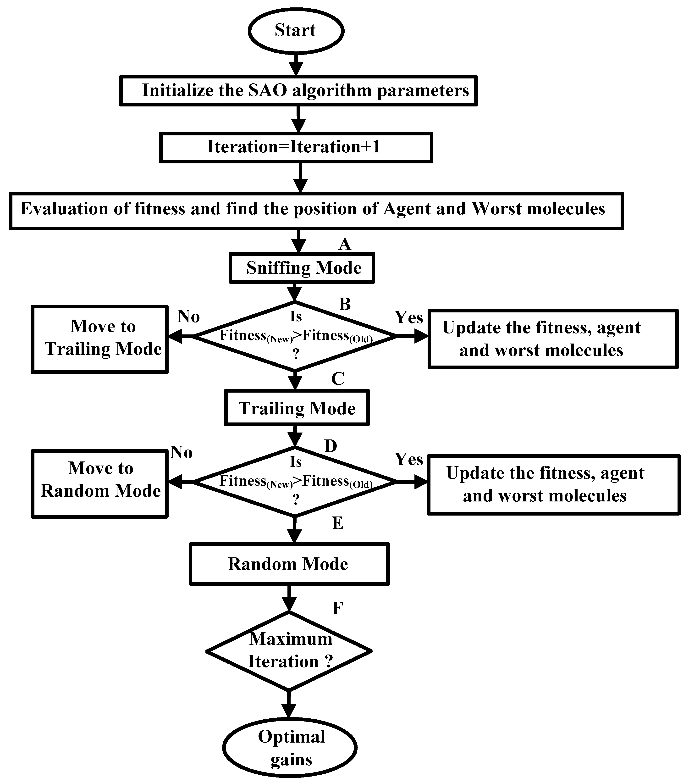
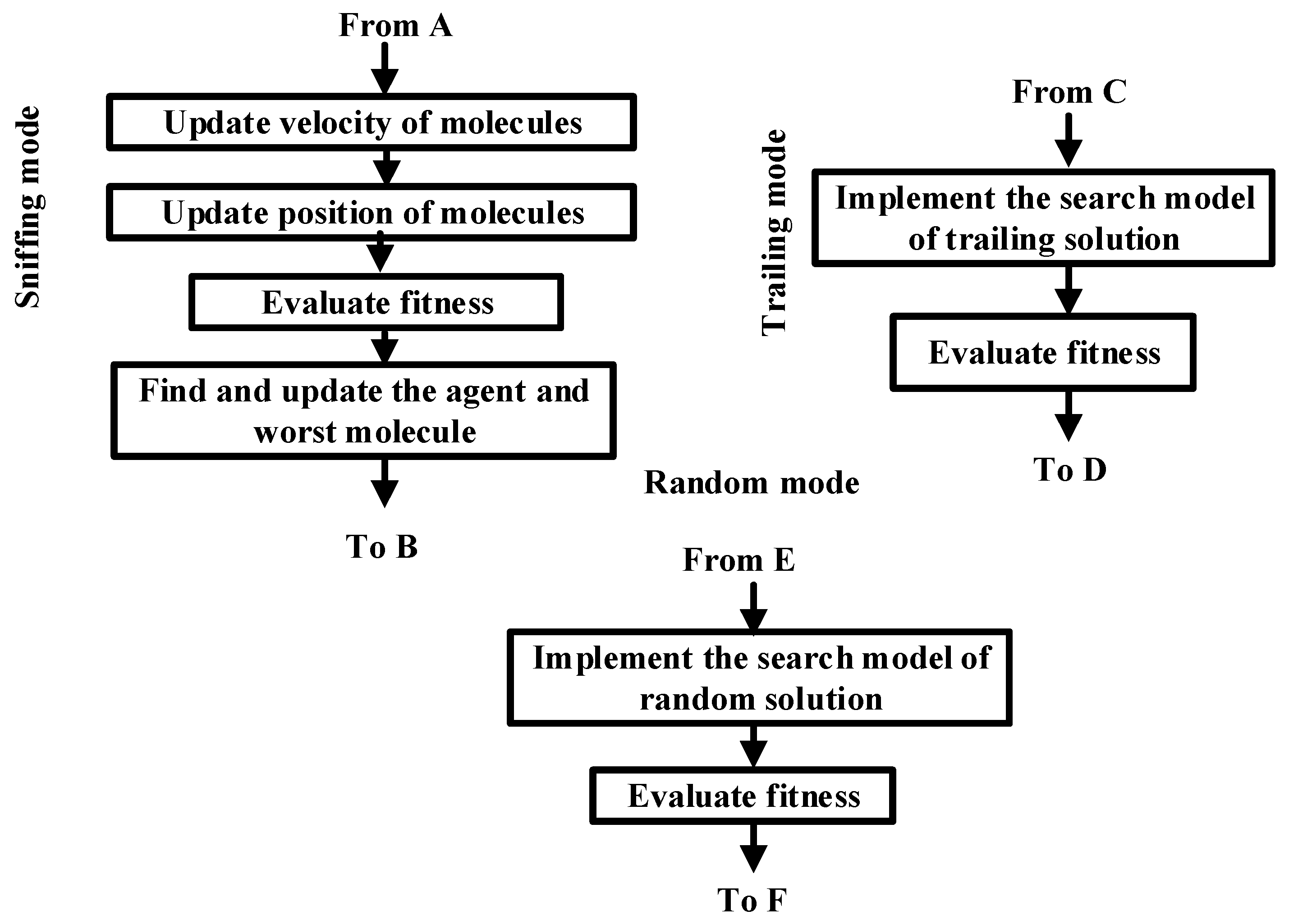
The rest of the manuscript is described as follows. In Section 2, the system considered for evaluation is described. The various controllers are explained in Section 3. The detailed SAO algorithm is discussed in Section 4. In Section 5, the analysis of the obtained results is discussed. Finally, the conclusions are described in Section 6.

2. System under Investigation

In the present manuscript, a multi-source interconnected micro-grid system is considered for investigation that has a biodiesel generator (BDG), a ship diesel generator (SDG), wind turbines (WTs), an aqua-electrolyzer, a fuel cell, a diesel generator (DG), electric vehicles (EVs), a biogas (BG) plant, and a storage system (battery energy storage (BES) and flywheel energy storage (FES)) in both areas. The effectiveness of various classical controllers (I, PI, and PID) in stabilizing/regulating the frequency and power is addressed. The nominal gain and time constant values of the various components considered are mentioned in Appendix A.

2.1. Electric Vehicle

There are basically three principal states of an EV, namely, driving, charging, and controllable states. After plugging in an EV, it enters into the driving state, and its state transitions from the controllable to the driving state. Each EV has a battery of 3 kW/15 kWh (C_kW = 3 and C_kWh = 15). After the trip, when the EV is plugged into a charging mode to charge its battery, this is referred to as the charging state of the EV. During this state of the EV, it is uncontrollable, i.e., it does not respond to frequency regulation (FR) signals. In the controllable state, the EV responds to FR signals, whereby the SOC of the EV fluctuates depending on the FR signal. The control-in rate is calculated using a random function so that the average of the driving period and energy loss from plug-out can be found. The charge and discharge of controllable EVs are limited by their MW (±C_kW) and MWh (80–90% of the SOC) limits. Each EV informs its local control center about its state of control, whether they are controlled-in or plugged-out. The model for the FR of EVs is given in Figure 1 [11]. This model replicates the behavior of one EV battery. This EV model can be used to calculate the total charging or discharging power in a controllable state. In Figure 1, The terms T, μ_e, and δ_e denote the time constant, inverter capacity, and power ramp rate constraints, respectively, of an EV. E_MAX and E_MIN denote the maximum and minimum controllable energy of the EV battery. ΔP_EV shows the amount of charging/discharging power. When ΔP_EV = 0, the EV is said to be in idle mode; if ΔP_EV > 0, the EV stays in discharging mode; and ΔP_EV < 0 means the EV is in charging mode. EVs can be charged and discharged within the limits of ±μ_e. However, it should be noted that when the stored energy of the EV exceeds the upper limit (E_MAX), the EV may no longer be charged, and, thus, it can only be discharged within the range of 0 to μ_e. Similarly, if the stored energy of the EV is less than the lower limit (E_MIN), the EV can only be charged within the range of −μ_e to 0. The terms K₁ and K₂ denote the difference between the limited energy and current energy of the EV battery, respectively, which can be estimated as K₁ = E − E_MAX and K₂ = E − E_MIN, respectively, where, E is the current energy of the EV battery.

Several EVs are used in a charging station; therefore, there is a need for considering an aggregate equivalent EV model that considers each EV with dissimilar inverter capacities, which is called the total energy model (TEM) of an EV. The TEM used for frequency regulation is shown in Figure 2 [3,29]. In the present study, a TEM with 50,000 EVs is assumed, in which 10% of them are treated as being in the vehicle-to-grid (V2G) controllable state. The EVs have a bidirectional nature and can be connected in either a series or parallel arrangement. If the EVs are charged, they respond to the load frequency control (LFC), i.e., frequency regulation (FR) signals within the energy capacity limits, i.e., the MWh limits expressed as $E_{CONTROL}^{MIN}\le E_{CONTROL}\le E_{CONTROL}^{MAX}$. The energy of the controllable EVs is denoted as $E_{CONTROL}$. The lower and upper energy capacity limits are represented by $E_{CONTROL}^{MIN}$ and $E_{CONTROL}^{MAX}$, respectively. These limits are estimated from Equations (1) and (2) and depend on the SOC, i.e., the control strategy [29].

$$E_{CONTROL}^{MIN}=\frac{N_{CONTROL}\ast C_{kWh}}{1000}\ast 0.8$$

(1)

$$E_{CONTROL}^{MAX}=\frac{N_{CONTROL}\ast C_{kWh}}{1000}\ast 0.95$$

(2)

The entire energy stored in all EVs, E_CONTROL, can be obtained from Equation (3), which shows the relation between the control-in energy (E_CONTROL-IN), plug-out energy (E_PLUG-OUT), initial energy (E₀), and energy associated with frequency regulation (E_FR).

$$E_{CONTROL}=-E_{FR}+E_{CONTROL\text{-}IN}+E_0+E_{PLUG\text{-}OUT}$$

(3)

The number of plug-out EVs is taken as 10,000 and that of the control-in EVs is taken as 40,000, and the initial SOC of the EVs in the TEM is considered as 0.8. The number of controllable EVs can be calculated with the help of the control-in rate (R_CONTROL-IN), the plug-out rate (R_PLUG-OUT) that denotes the number of EVs entering the controllable state, and the number of initial controllable EVs (N₀), as shown in Figure 3.

2.2. Biodiesel Generator [30]

Biodiesel is an esterified product, which can be obtained from biofuel basics (sugar, starch, or vegetable oil). It is an environmentally friendly and sustainable source of energy, and, hence, it does not affect the environment in a negative manner. The first-order transfer function of a biodiesel generator is given using Equation (4).

$$\mathrm{Biodiesel} \mathrm{Generator}: G_{BDG}=\frac{K_{VA}·K_{BE}}{(1+s{T}_{VA})(1+s{T}_{BE})}$$

(4)

2.3. Storage System [9]

A battery energy storage system (BESS) is used to manage short-term power fluctuations, which can occur in a micro-grid due to various unavoidable reasons. The BESS effectively handles these situations to keep the frequency variation within suitable limits. The time constants of a BESS are limited to several seconds as it takes time to charge. On the other hand, a flywheel energy storage system (FESS) plays a crucial role in supplying the requisite energy in peak load periods quickly by storing energy in a kinetic energy form during off-peak periods. The linearized transfer functions are denoted in Equations (5) and (6).

$$\mathrm{Battery} \mathrm{storage}: G_{BES}=\frac{K_{BESS}}{1+s{T}_{BESS}}$$

(5)

$$\mathrm{Flywheel} \mathrm{storage}: G_{FES}=\frac{K_{FES}}{1+s{T}_{FES}}$$

(6)

2.4. Ship Diesel System [27,31]

Due to several advantages, such as a quick start, high efficiency, and minimum maintenance, a ship diesel system (SDG) acts as the backup choice for shipboard micro-grids. Uncontrollable oscillations in a micro-grid system can be effectively controlled using an SDG [31], whose first-order transfer function is given using Equation (7) [27].

$$G_{SDG}=\frac{1}{(1+s{T}_g)(1+sT)}$$

(7)

2.5. Wind Turbine Generator (WTG) [9]

A WTG is a renewable resource, and its power generation depends on the speed of wind, as expressed in Equation (8).

$$P_{WT}=\frac{1}{2}\rho A_r{C}_P{V}_W^3$$

(8)

where $\rho$, $A_r$, $C_P$, and $V_W^3$ are the air density (=1.25 kg/m³), blades’ swept area, power coefficient, and cube of wind speed, respectively. The linearized WTG model is given using Equation (9).

$$G_{WT}=\frac{1}{1+s{T}_{WT}}$$

(9)

2.6. Aqua-Electrolyzer (AE) and Fuel Cell (FC) [9,32]

An aqua-electrolyzer (AE) uses a part of a WTG to produce hydrogen gas, which is used for the generation of power in a fuel cell (FC). A fuel cell uses the chemical energy of hydrogen to generate electricity by combining air with gaseous hydrogen in the absence of combustion. FCs offer several advantages, such as a low pollution level, high efficiency, etc. [32]. The small-signal representations of AE and FC are given using Equations (10) and (11).

$$G_{AE}=\frac{K_{AE}}{1+s{T}_{AE}}$$

(10)

$$G_{FC}=\frac{K_{FC}}{1+s{T}_{FC}}$$

(11)

2.7. Diesel Generator (DG) [11]

A DG produces power on a small scale and has advantages such as a high starting speed, durability, and higher efficiency. When load demand varies, a DG adjusts its output and contributes to frequency stabilization through fuel regulation [11], whose linearized transfer function is given using Equation (12).

$$G_{DG}=\frac{K_{DG}}{1+s{T}_{DG}}$$

(12)

2.8. Bio-Gas Generator (BGG) [15]

Biogas is produced by biochemically compositing the organic waste in O₂-free environments, which can be utilized as a substitute for existing traditional DGs. The small-signal-based transfer function of a BGG is given in Equation (13).

$$G_{BGG}=K_{BG}\frac{1+s{X}_c}{(1+s{Y}_c)(1+s{b}_B)}·\frac{1+s{T}_{CR}}{1+s{T}_{BG}}·\frac{1}{1+s{T}_{BT}}$$

(13)

The micro-grid under study is shown in Figure 4, in which different controllers are applied to obtain a better system stabilization of oscillations subjected to the minimization of the figure of merit J_MIN given using Equation (14).

$$J_{MIN}={\displaystyle \underset{0}{\overset{Time}{\int }}\{\Delta f_1^2+\Delta f_2^2+\Delta P_{tie}^2\}dt}$$

(14)

where $\Delta f_1^2$, $\Delta f_2^2$, and $\Delta P_{tie}^2$ denote the squares of the variations in the frequencies in areas 1, 2, and the tie-line power connecting these areas.

3. Controllers Utilized

In the present study, to stabilize/regulate the oscillations, the classical controllers named integral (I), proportional plus I (PI), and PI plus derivative (PID) are applied in both control areas. The I controller has one tunable parameter (K_I), the PI controller has two parameters, (K_I and K_P), and the PID controller has three tunable knobs (K_I, K_P, and K_D). These classical controllers’ structures are shown in Figure 5. The PID control process can be described in the time domain as Equation (15).

$$R(t)=K_{P}ACE+K_I{\displaystyle \int ACEdt}+K_D\frac{d}{dt}ACE$$

(15)

where, ACE denotes the area control error, which is the combination of the changes in the frequency (Δf) and tie-line powers (ΔP_tie), and R(s) is the output of the controller.

In the Laplace domain, it can be written as Equation (16) or Equation (17).

$$R(s)=K_{P}ACE+\frac{K_I}{s}ACE+s{K}_{D}ACE$$

(16)

$$\frac{R(s)}{ACE}=K_P+\frac{K_I}{s}+s{K}_D$$

(17)

4. SAO Algorithm

The SAO algorithm is a recent optimization technique proposed by Salawudeen et al. [28]. It is based on the connection between smell agents and the objects that evaporate the smell molecules. This SAO algorithm is governed by three modes, namely, sniffing, trailing, and random. In the sniffing mode, the agent distinguishes smell molecules, finds their positions, and makes the decision to find the source or not. In the trailing mode, based on the conclusion from the sniffing mode, the agent follows the smell molecules. The random mode helps the agent in avoiding the local optimum solutions. The SAO algorithm flow chart is given in Figure 6, and its processes are given in Figure 7.

4.1. Sniffing Mode

The initialization of smell molecules is given using Equation (18).

$$X_i^{(m)}=\left[\begin{array}{ccc}{x}_{(1,1)}& x_{(1,2)}& x_{(1,D)}\\ ⋮& ⋮& ⋮\\ x_{(N,1)}& x_{(N,2)}& x_{(N,D)}\end{array}\right]$$

(18)

The terms N, D, and m denote the total number of variables, decision variables, and iteration count, respectively.

The best position of the agent can be generated using Equation (19).

$$X_i^{(m)}=LB+r_0\times (U{B}_i-L{B}_i)$$

(19)

where LB, UB, and r₀ denote the lower and upper bounds and random value ∈ (0,1].

The velocity with which smell molecules diffuse from the origin or source is given using Equation (20).

$$v_i^{(m)}=\left[\begin{array}{ccc}{v}_{(1,1)}& v_{(1,2)}& v_{(1,D)}\\ ⋮& ⋮& ⋮\\ v_{(N,1)}& v_{(N,2)}& v_{(N,D)}\end{array}\right]$$

(20)

The Brownian-form diffused molecule velocity updating is performed using Equation (21).

$$x_i^{m+1}=x_i^m+v_i^{m+1}\times \Delta t$$

(21)

where Δt assumed to be 1.

The velocity update in the smell molecules is evaluated using Equation (22).

$$v_i^{t+1}=v_i^t+v$$

(22)

where the updated component of the velocity, v, is given using (23).

$$v=r_1\sqrt{\frac{3kT}{M}}$$

(23)

where k, M, and T denote the smell constant, the mass of the molecule, and the temperature, respectively.

4.2. Trailing Mode

This mode models the searching nature of the agents toward smell sources. The agent motion towards smell sources is given using Equation (24).

$$x_i^{m+1}=x_i^m+r_2\times olf\times (x_{agent}^m-x_i^m)-r_3\times olf\times (x_{worst}^m-x_i^m)$$

(24)

The notations r₂ and r₃ are random numbers ∈ (0,1] that penalize the influence of the olfaction capacity (olf) on $x_{agent}^m$ and the effect of olf on $x_{worst}^m$.

4.3. Random Mode

The random motion of the smell agent is given using Equation (25).

$$x_i^{m+1}=x_i^m+r_4\times SL$$

(25)

where, SL denotes the step length, and r₄ is a random value that penalizes r₄.

For the optimization of the various parameters of the classical controllers, the SAO algorithm parameters considered are olf = 0.9, k = 0.6, M = 0.9, T = 0.95, SL = 0.02, the smell molecule number (N) = 5, and iterations (m) = 100 subjected to obtain J_MIN discussed in Equation (14).

5. Analysis of Results

5.1. Nominal Conditions

This case study is evaluated in the MG system (Figure 4) with consideration of a 2% step-natured disturbance (SND) in both areas. With a 2% SND, the parameters of the classical controllers, namely, I, PI, and PID, are tuned using the SAO algorithm and are given in

Table 1. The SAO-tuned I, PI, and PID controllers’ parameters.

Parameter/Controller	I	PI	PID
KP (Area 1)	-----	0.9980	0.9080
KI (Area 1)	0.3644	0.869	0.9200
KD (Area 1)	-----	-----	0.8170
KP (Area 2)	-----	0.2277	0.8660
KI (Area 2)	0.1450	0.9989	0.9912
KD (Area 2)	-----	-----	0.9500

. With these values, the regulation of frequency and tie-line power changes are plotted and compared in Figure 8. The various measures of performance such as settling duration (SD), highest magnitude (HM) and lowest magnitude (LM) of oscillations are indicated in

Table 2. The settling durations and highest and lowest magnitudes of Figure 8 responses.

Response/Dynamic Measures	Settling Duration			Highest Magnitude (10−3)			Lowest Magnitude (−10−3)
	I	PI	PID	I	PI	PID	I	PI	PID
Response, Δf1	15.93	12.45	10.36	18.54	15.59	12.95	13.44	9.89	8.97
Response, Δf2	8.699	8.272	8.187	34.65	18.52	18.42	16.28	12.91	11.58
Response, ΔPtie	21.57	20.63	17.66	03.64	02.52	0.73	0.38	0.35	0.16

among these controllers.

It is clear from Figure 8 and Table 2 that between the three classical controllers, the PID controller is superior in terms of the SD, HM, and LM measures. The critical evaluations of the results for this case are explained herein.

The Δf (Area 1) graph shows a 53.76% and 20.17% improvement in the SD with PID in comparison with the I and PI controllers. With the PID controller, a 6.25% and 1.03% superior response in the SD of Δf (Area 2) is witnessed compared with the I and PI controllers. Similarly, the settling durations (SDs) are improved by 22.14% and 16.81% compared with earlier controllers for ΔP_tie.

The highest magnitudes (HMs) of oscillations are reduced by 43.16% and 20.38% in Δf (Area 1) and 88.11% and 0.542% in Δf (Area 2) for the PID controller compared with the I and PI controllers. The effectiveness of the PID controller is found in the lowest magnitudes (LMs) of oscillations, measured as 49.83% and 10.25% in Δf (Area 1) and 40.58% and 11.48% in Δf (Area 2) with the other controllers.

A comparative scrutiny is evaluated between these controllers in view of their convergence behavior. In Figure 9, the convergence characteristics are plotted, and it can be witnessed that the PID controller not only converges quickly but also provides a minimum objective function value (J_MIN) compared with the other controllers. A magnitude analysis is represented in Figure 10 to support this statement.

5.2. Varied Load Demand Pattern

In the above Section 5.1, the step-natured disturbance (SND) is considered as the load. However, in practice, the disturbance in the micro-grid system varies continuously. To analyze the performance of the I, PI, and PID controllers in the event of a continuously varied load demand, randomized-nature disturbance (RND), as shown in Figure 11, is applied as the disturbance in Area 1. With the RND as the load demand, the I, PI, and PID controllers’ parameters are again tuned with the SAO algorithm and given in

Table 3. The SAO-I, SAO-PI, and SAO-PID parameters with RND.

Title 1	I	PI	PID
KP (Area 1)	-----	0.9900	0.3700
KI (Area 1)	0.9980	0.8690	0.9990
KD (Area 1)	-----	-----	0.5810
KP (Area 2)	-----	0.2277	0.2660
KI (Area 2)	0.9050	0.9980	0.2199
KD (Area 2)	-----	-----	0.9970

. With these numerical values, the dynamic responses among these controllers are plotted and compared in Figure 12. Critical observations of these dynamics prove the efficiency of the PID controller in view of the HM, LM, and oscillations compared with the I and PI controllers.

5.3. Evaluation of Performances of SAO, FA, and PSO Techniques

In all the above studies, the SAO algorithm is used to tune all the parameters of the controllers. Herein, an attempt is made to compare the SAO algorithm with the recently used firefly algorithm and particle swarm optimization methods. From the above studies, the superior PID controller is taken for this purpose, and its parameters are individually obtained with all these controllers and shown in

Table 4. The PSO-PID and FA-PID controller parameters.

Parameter/Algorithm	PSO	FA
KP (Area 1)	0.9129	0.9995
KI (Area 1)	0.4387	0.9998
KD (Area 1)	0.7006	0.9171
KP (Area 2)	0.6616	0.9998
KI (Area 2)	0.8262	0.4220
KD (Area 2)	0.8553	0.9979

(the SAO-PID values are already given in Table 1). The convergence nature of PSO [33]-PID and FA [34]-PID are evaluated against the proposed SAO-PID in Figure 13. The critical evaluation in Figure 13 shows that SAO-PID provides quick convergence along with a minimized J_MIN, which confirms the efficiency of SAO-PID compared with FA-PID and PSO-PID.

5.4. Insensitiveness of SAO-PID Parameters

From the above studies, the SAO-PID is found to be superior to all the other controllers. However, it is expected that the system conditions will change, and in those changed conditions, whether SAO-PID retains its efficiency or not is tested in this case. For this, in this section, two types of investigations are performed: firstly, with larger load demands and later, with variations in the time constant of the WTs.

5.4.1. In Larger Load Demand Condition

In this condition, the PID controller is judged for its insensitiveness with larger load demands in the control areas. In nominal conditions, the assumed SND is 2% in both areas. The SND values are raised to 3% and 5% in control areas 1 and 2, separately. With these larger amplitudes of SND, the PID controller parameters (K_P, K_I, and K_D) are again tuned using the SAO algorithm, and the values are shown in

Table 5. The SAO-PID gains at different magnitudes of SND.

Parameter/SND Magnitude	3% SND	5% SND
KP (Area 1)	0.3700	0.9650
KI (Area 1)	0.9980	0.9800
KD (Area 1)	0.5810	0.8900
KP (Area 2)	0.2660	0.8600
KI (Area 2)	0.2199	0.9760
KD (Area 2)	0.9900	0.9890

. With these numerical parameters, the obtained dynamics are compared with those responses plotted using the optimum gains given in Table 1 in Figure 14 and Figure 15.

In Figure 14 and Figure 15, it is seen that the responses with the nominal and obtained parameters are not deviating too much, i.e., they are almost the same, which proves the insensitiveness (robustness) of the optimal PID parameters obtained at the nominal SND (2%) for wide variations in SND (3% and 5%).

5.4.2. With Changed Time Constants of WTs

In this study, the time constant (T_WT = 1.5 s) of intermittent WTs is changed by ±25%, i.e., to 1.125 s and 1.875 s, and, again, the PID parameters are tuned with the SAO algorithm, separately, for 1.125 s and 1.875 s and are shown in

Table 6. The SAO-PID gains for ±25% deviations in T_WT.

Parameter/% Change in TWT	−25%	+25%
KP (Area 1)	0.5800	0.7300
KI (Area 1)	0.8510	0.9900
KD (Area 1)	0.7810	0.8010
KP (Area 2)	0.9200	0.9160
KI (Area 2)	0.6800	0.6200
KD (Area 2)	0.9960	0.8300

. In these changed conditions, i.e., T_WT = 1.125 s and T_WT = 1.875 s, the dynamics are compared with the nominal WT time constant value (T_WT = 1.5 s) using the gains given in Table 1 and are shown in Figure 16 and Figure 17.

The observations of the comparative dynamics shown in Figure 16 and Figure 17 reveal that they are almost identical, which proves the stiffness of the SAO-PID parameters against wind turbine generator time constant (T_WT) variations by ±25%.

6. Conclusions

In this article, the frequency stabilization/regulation issue is performed using a smell agent optimization (SAO)-algorithm-based PID, i.e., a SAO-PID controller in a micro-grid system comprising wind turbines, an aqua-electrolyzer, a fuel cell, a biogas plant, a bio-diesel plant, diesel generation (DG), ship DG, electric vehicles, energy storage devices, flywheels, and batteries. The prime findings of the present research are as follows:

• The SAO-PID controller performs well when compared with the SAO-PI and SAO-I controllers in view of the settling duration and highest and lowest magnitudes of oscillations.
• The minimum cost function value is evidenced with the SAO-PID controller in comparison with the SAO-based I and PI controllers.
• The efficacy of the SAO-PID controller is observed for randomized-nature disturbance, also in view of the minimal highest and lowest magnitudes of deviations.
• The SAO technique performance was found to be efficient compared with the PSO and FA techniques with the measures of both convergence and minimum cost values.
• The parameters of the SAO-tuned PID controller obtained at nominal conditions are insensitive for larger amplitudes of step-natured disturbances.
• The SAO-based PID controller parameters were found to be stiff for wide variations in the time constant values of wind turbines by ±25%.

Future Scope

This study can be extended with the utilization of intelligent controllers such as fuzzy logic and neural network controllers for further effective frequency regulation in micro-grids. The various degrees-of-freedom controllers, namely, the two-degrees- and three-degrees-of-freedom controllers, can also be implemented for the above study. Generalized PID controllers, so-called fractional-order controllers, can be applied for effective frequency stabilization/regulation in a micro-grid system. The selection of the gains of these controllers can be performed using other optimization methods that can perform better than the SAO technique in providing optimal solutions.