
Development and Verification of Novel Building Integrated Thermal Storage System Models
by
 , ,
, ,
Matthias Pazold
1,
Jan Radon
1,2,
Matthias Kersken
3,
Hartwig Künzel
3,*,
Florian Antretter
1 and
Herbert Sinnesbichler
3 1
C3RROlutions GmbH, 83064 Raubling, Germany
2
Faculty of Environmental Engineering, University of Agriculture, 30-239 Kraków, Poland
3
Fraunhofer Institute for Building Physics, 83626 Valley, Germany
*
Author to whom correspondence should be addressed.
Energies 2023, 16(6), 2889; https://doi.org/10.3390/en16062889
Submission received: 16 February 2023
/
Revised: 15 March 2023
/
Accepted: 16 March 2023
/
Published: 21 March 2023
(This article belongs to the Special Issue Energy Efficiency of the Buildings II)
Abstract
:In electrical grids with a high renewable percentage, weather conditions have a greater impact on power generation. This can lead to the overproduction of electricity during periods of substantial wind power generation, resulting in shutoffs of wind turbines. To reduce such shutoffs and to bridge periods of lower electricity production, three thermal energy storage systems (TESs) have been developed for space heating and domestic hot water. These include a water-based thermal system (WBTS), a thermally activated building system (TABS), and a high-temperature stone storage system (HTSS). The paper explains the development of computer models used to simulate the systems and their successful verification using field measurements. Target values to cover about 90% of building heating demand with excess electricity were found to be achievable, with performance ratios depending on storage size, particularly for WBTS and HTSS. The TABS’ storage capacity is limited by building geometry and the available inner ceilings and walls.
1. Introduction
The share of electricity from renewable energy in the national power grids has increased significantly in most countries in recent years and will continue to grow. Solar and wind power supply are, unlike conventional power, less demand-controlled, because they depend a lot on weather conditions [1]. In Germany, wind power meanwhile accounts for the largest share of renewable electricity production [2]. Consequently, there is a high proportion of volatile energy in the electricity mix. At times of strong winds, more electricity may be produced than temporarily can be consumed or transported over long distances. Thus, wind turbines must be switched off to avoid overloading the electrical grid [3] which leads to costly redispatches. In Germany, the share of wind power is particularly high in winter due to the frequent occurrence of strong wind events. An analysis of the weather conditions has shown a 95% probability of strong wind events, which last on average 9 h within a period no longer than 13 days in average German winters [4]. As a result, storage options to utilize the energy with such a production pattern will further gain importance.
Research from [5] is related to the systems for energy storage methods and their application in power production facilities and plants. Besides thermal energy storage (TES), there is gravitational energy storage such as pumped hydroelectric storage (PHES), compressed air energy storage (CAES), mechanical by flywheel rotation energy, electromagnetic storage (SMES), and power to gas systems such as hydrogen generation (electrochemical accumulation) which release heat via gas combustion or electricity via fuel cells. The authors conclude that PHES, thermochemical energy storage (TCES), and thermo-capacity storage including water heat tanks and phase transition are promising with their main advantage being their low capital costs for power production facilities and plants. For energy storage in buildings, PHES is less relevant for single buildings and is geographically limited and storing electricity in lithium-ion batteries is too expensive for multi-day storage [6].
In cold climates, buildings require thermal energy, which can be provided by power to heat systems. Thermal energy storage allows for the partial decoupling of the energy generation from actual energy consumption, making use of surplus electricity to sustain a period of time without energy from fossil fuels. This leads to load reduction and obviously to a reduction in CO2 emission [7].
The method of storing energy determines the heat quantity and its usage time. Passive heat buffering in assemblies surrounding conditioned space depends on their thermal storage capacity, which can be increased via latent heat storage and the usage of phase change materials (PCMs). Different PCMs have been investigated using different experimental methods [8]. Research results show positive effects for heating energy savings [9] under fluctuating outdoor weather conditions. For a high heat exchange rate, another viable, active system interacting with PCM is necessary [10]. Unlike PCMs, the sensible heat storage capacity of conventional TES is more limited by minimum and maximum temperature levels, at least if no heat pump is used. In the case of water storage, the maximum temperature limitation is the boiling point temperature. Thus, more capacity requires an increase in volume. Regarding different materials that are as sensible as TES, the volumetric thermal storage capacity is reviewed according to its advantages and challenges when applied to zero energy buildings in [11]. Using a heat pump can shift the operational temperature of the storage material to the necessary comfort temperatures during the unloading of the storge; however, additional power is required to create this shift. As an electricity accumulator, the air source heat pump with added thermal energy storage (ASHP-TES) can shift the operation to times with better weather conditions [12]. However, using large amounts of electricity in a short time period is not an application case for heat pumps. Besides short-term storage, seasonal sensible, latent, and chemical storage [13] for residential buildings have also been investigated. A more detailed example of a borehole thermal storage system (BTES) is given in [14].
In general, innovative energy technology is necessary and required [15], but evaluated TES systems, such as in [16], mainly cover seasonal or diurnal periods but lack the analysis of TES that sustains a period of multiple days in residential buildings. The research and modeling of TES based on wind energy production patterns are little described in the literature. In this paper, the use of excess energy in the electrical grid to cover the heat and domestic hot water demand in buildings for weather patterns as explained above, i.e., for multiple days, is investigated. Only energy conversion from electricity to thermal energy is assumed; so, only TES is investigated. Residential thermal storage systems, investigated in [17], might only need to be enlarged. The authors concluded that such systems are used to shift peak loads and increase part of renewable energy, but differences in the thermal envelope between new construction and renovated buildings will become more important. There are well-known short-term storage heaters [18], placed in single rooms, using electricity at night to heat ceramic bricks which release thermal energy during the following day, formally used to exploit the excess electricity at night and balance the load in the grid. These are also improved by insulation to release less uncontrolled passive heat dissipation or used the other way around to be heated during the day via photovoltaics and release the heat at night [19].
However, for a thermal storage system which uses only surplus renewable electricity, while avoiding additional stress to the grid, various aspects need to be examined. The basic sizing of the storage technology will need to be designed to charge energy within a time frame of 9 h and to bridge a period of 13 days with the stored heat, i.e., something in between short-term and seasonal TES. Another key requirement is to use well-known and available market technologies, embeddable in new or retrofitted buildings. Regarding ecological and economical points of view, three systems were identified to be promising [4], including water-based thermal storage (WBST) with enough water volume to cover the heating demand of the building for several days. Another system use the available massive building components through their thermal activation (TABS) by adding a little insulation layer to control the heat flow to the rooms. The last system is a centralized high-temperature stone storage (HTSS). These systems are described and discussed in [20,21] and the results about their overall performance are discussed. To investigate the behavior of these systems, prototypes were built and evaluated. To enable a more general evaluation of these systems, with a broad variety of building types, usage, system specifics, and location, among others, the simulation of the systems integrated in the building is necessary. The simulation needs to be detailed enough to represent the system dynamics in direct interaction with the building to calculate the heat demand covered by the excess electricity but also the thermal comfort. In addition, the simulation needs to be fast enough for parametric studies and its application in the design process of such buildings. Monthly energy balance calculations are not applicable to investigate the dynamic behavior and thermal comfort in buildings [22]. Computational fluid dynamic (CFD) software could model the storage system in a very detailed way and can be coupled to building simulation software. However, this comes with a high computational cost [23], and therefore it is less applicable to extended simulation studies. An existing building simulation tool [24] is supplemented via the dynamic simulation of the technology to fill the gap in between monthly balance calculations and CFD.
2. Thermal Storage Concepts
All considered thermal storage comes with passive thermal losses. The insulation levels of all three storage systems are sized to meet the heating load of a high-performance building. Thus, the storage losses are not wasted but can fully contribute to space heating. All considered storage can be applied to new and also to retrofitted buildings, as long as their envelope and ventilation heat recovery are those of a high-performance building in terms of heating demand.
2.1. Load Control
An automated control takes care to fit the charging levels to the predicted heating demand so that the losses can also be utilized in warmer weather. First, weather forecast data are used to predict strong wind events as well as to estimate the heating demand of the building. The system only charges enough energy to meet the heating and domestic hot water demand estimation until the next predicted charging event. This is necessary to prevent fully loaded storage with undesired high passive heat losses.
In addition, the price of electricity is considered. Electricity prices on the day ahead and the intraday market indicate the share of renewable energies from which a market signal is derived. In times of surplus electricity, the stock market price of electricity decreases. This can even lead to negative prices. In this case, the purchase of electricity is not only favorable for the consumer, but it also stabilizes the market [25]. In the last step, the grid load between the production and the consumption location is analyzed to ensure that the required grid capacities are available. Finally, all of this information is used to generate a signal that determines the charging process of the thermal storage capacities in the building [26].
2.2. Hot Water Tank
The first technology introduced and investigated uses the excess electricity and stores it as thermal energy in water-based thermal storage (WBTS). The water in the tank is heated and stratified by a powerful direct electric-flow-type heater. Domestic hot water (DHW) is supplied by a DHW exchange module connected to the hot water tank. Whenever the storage temperature is lower than the design temperature for DHW, a small electric flow water heater raises the temperature to the desired setpoint temperature. Space heating is carried out via a common building heat transfer system with low supply temperatures, such as panel heating. The inlet temperature for the building heat transfer system is raised by another electric flow water heater whenever the desired temperature is not achieved by the storage temperature. Both small additional water heaters are introduced to prevent the unwanted heating of the WBTS’s large volume, if no excess electricity is available. The dimension and the water volume of the tank, respectively, can be determined by a newly developed procedure called the “wind period method” [20]. The tank should be well insulated to minimize the passive heat dissipation through the storage walls. The principal scheme of the hot water storage tank system is shown in Figure 1.
2.3. Building Components as Thermal Storage
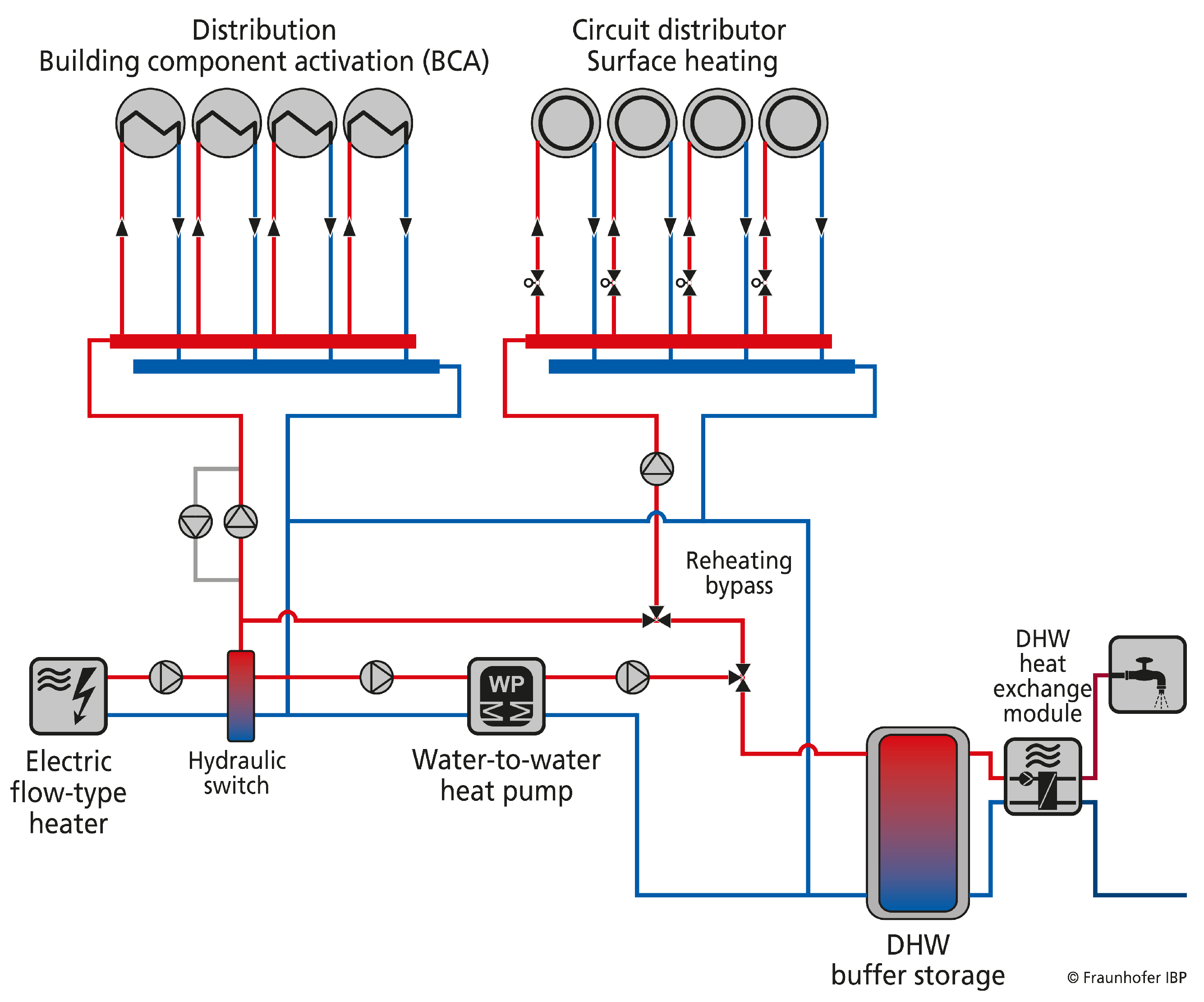
Usually, a thermally activated building system (TABS) is used for the continuous building conditioning, to reduce maximum heating and cooling loads by using the thermal inertia of building components and to keep the component surface temperatures comfortable. The TABS is supplied with warm or cool water in such a way that the return temperature of the TABS is approximately in the middle of the target temperature corridor for the room air temperatures (return temperature control). This temperature control within the target corridor creates the so-called self-regulating effect. If the room air is cooler than its target value, the TABS releases heat to the room air; if the room air is warmer, it is cooled by the TABS. For the purpose of storing excess electrical energy, the newly introduced concept uses the TABS to store heat at a significantly higher temperature level in order to store the required energy. Due to the increased temperature level, the self-regulating effect of such systems will not work. To ensure that the temperature difference between the storage building mass and the room air does not lead to the unwanted overheating of the rooms, a certain decoupling of the TABS storage masses from the room air becomes necessary. Insulating the activated component shall reduce the uncontrollable passive heat dissipation and enable the active discharge of the ceilings into the room air. This is achieved through a thicker than common impact sound insulation layer on top of the concrete slab and additional insulation layers at the bottom of the component.
In general, both ceilings and partition walls can be used as TABS storage if they are made of a material with sufficiently high thermal mass and thermal conductivity. Heat storage in components of the building-envelope-facing exterior conditions should be avoided, if possible, even in the case of very energy-efficient envelopes, since the increased temperature difference between the inside and the outside would increase the transmission heat losses of the building. Within the scope of this research project, systems for new buildings with piping in the concrete molds as well as solutions for building renovation are considered. The system for renovation uses aluminum profiles with pipes, which are clad to the components’ surfaces covered with an additional insulation layer.
To charge the components with available excess electricity, a powerful direct electric-flow-type module water heater is used. Whenever the passive heat dissipation of the component is not enough to keep the indoor climate above the setpoint temperature anymore, a pump is activated to recirculate the water from the piping inside the component to an additional panel heating system outside of the insulation. Whenever the temperature in the component’s core becomes lower than the setpoint inlet temperature for the panel heating, a water-to-water heat pump is activated to increase the water temperature level. The energy source, or primary side for the heat pump, is the component core of the TABS. This heat pump is also used to prepare domestic hot water, because the setpoint temperature for DHW is above the component core temperature. Whenever the component core temperature falls below the lower limit (about 17 °C), the electric water heater is used to keep the design temperatures. The principal scheme of the thermally activated building storage system is shown in Figure 2.
2.4. High-Temperature Stone Storage
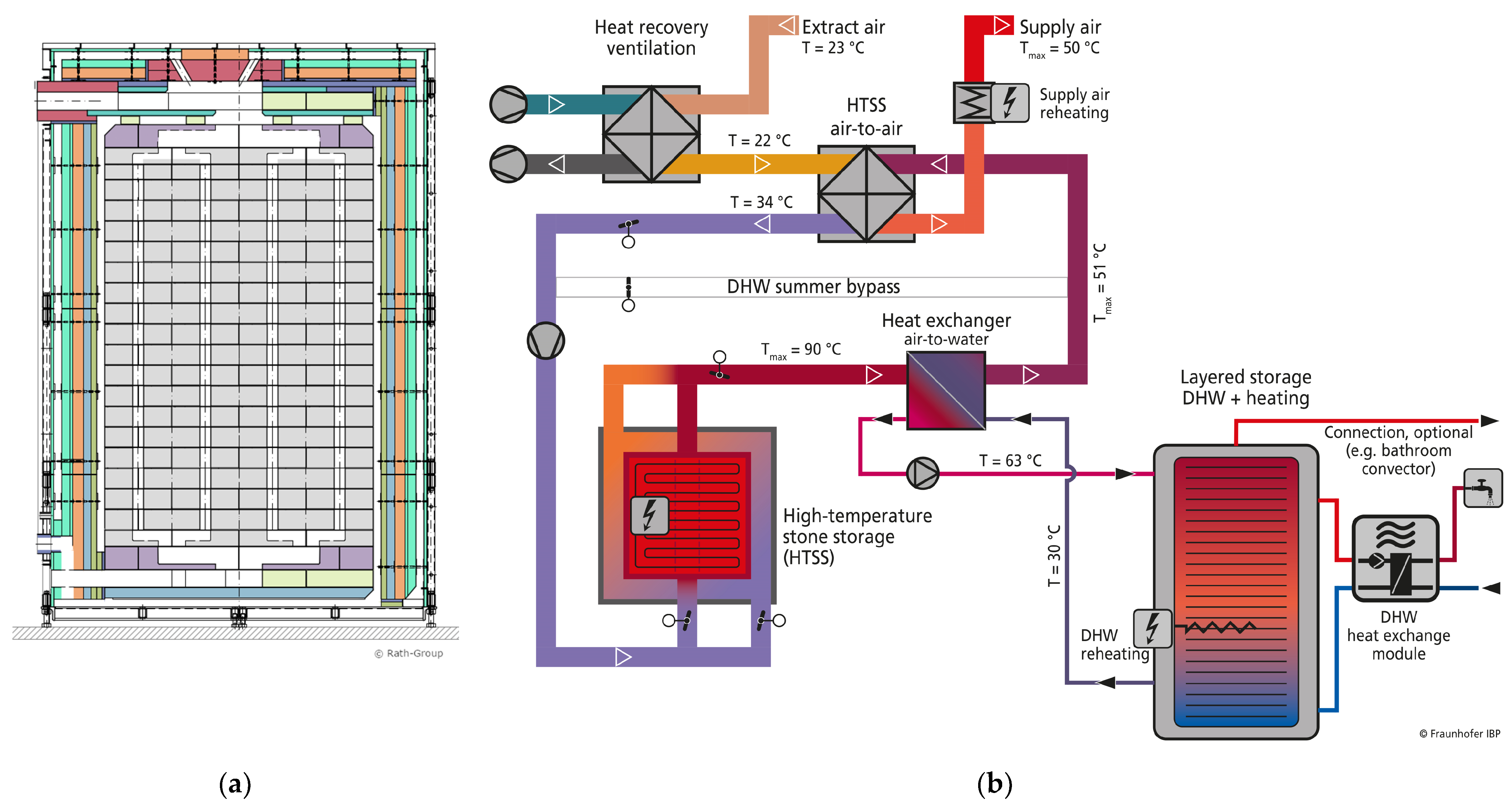
In this concept, the heat is stored in a massive “stone” core made of fired ceramic bricks and well insulated by layers of different insulation materials. The interior insulation layer must resist the high temperature of the core, which is about 800–900 °C. Additional insulation layers around the interior insulation can be less temperature-resistant, which also means being less expensive. A technical drawing is presented in Figure 3a. An aspect to be considered during the development of the stone storage is the handling of the approx. 5000 kg core material, typically installed in the cellar of a building. For this reason, the maximum weight of all individual components is limited to 9 kg, to be carried by humans. Accordingly, the insulated shell of the storage is modular, and the stone core is supplied as individual bricks and mortar.
The amount of heat necessary to charge the stone storage within a few hours to sustain the heat demand of the building for longer periods is supplied via electric heating rods. This requires the distribution of the charging power of approx. 50 kW depending on the building, and on the number and power of the heating rods in the stone core. If the number of the heating rods is too low, the storage will not be charged homogeneously and thus not completely, since the heat will not reach the stone volumes between the heating rods in the short time available. However, a very high number of heating rods leads to more cavities in the stone core, and increases the overall storage volume to provide the necessary thermal capacity. In addition, there is penetration in the storage insulation due to the electrical connection of each heating coil, whereby more heating rods also increase the storage losses.
While the storage is charged by the heating rods, the controlled heat output is realized by an air flow gap around the core. Regarding the ducts, it is also true that the optimum spacing or size is decisive for the function of the HTSS. Too few ducts prevent the use of the stone volumes between the ducts and, due to the small cross-section, generate high pressure losses in the air volume flow. Too many ducts mean a loss of thermal (stone) storage mass. The brick core is supplemented by air ducts below and above it. In order to distribute the air supplied to the storage core from the central connecting piece to the individual air channels in the core, a distribution layer of high-temperature resistant ceramics is used below the thermal core. Above the thermal core, the same layer is arranged but inverted to recollect the heated air before it leaves the hot stone.
In addition to the flow through the core, which is used for active heat extraction, an outside air gap between the core insulation and external shell is added. The air flow through this gap, the purge air gap, is controlled and used to keep the outer shell surface temperature low. It also feeds the passive storage losses of the HTSS to the building ventilation system and, thus, makes them usable. By means of an appropriately controlled ventilation flap, the total air volume flow is divided between the purge air gap and the core air channels in such a way that the outlet temperature desired by the control is established at the common air outlet of the HTSS. For safety reasons, it must be limited to a maximum of 90 °C.
This high temperature storage system is integrated into the building’s HVAC system, as shown in Figure 3b. After the HTSS, there is an air-to-water heat exchanger used for hot water preparation in a small tank. Space heating with this system is preferably performed through the mechanical ventilation system of the building, by heating the supply air. After the usual heat recovery heat exchanger, there is another air-to-air heat exchanger crossing the air flows from the building supply flow and the HTSS air circuit. Whenever the temperature of the supply air or the temperature in the small water tank fall below the setpoint temperature, there is additional direct electric heat via an air heater or the heating rod in the water tank.
3. Experimental Research
The development of hardware and control software of the storage system was aided by an extensive two-phase measurement campaign. During the pretest phase, the storage systems were loaded and discharged with stationary boundaries to be able to evaluate their performance and generate validation data for the simulation models. The second in situ phase included real boundaries such as climate and synthetic users, primarily to evaluate and optimize the control system. Since this paper describes the validation and calibration of the storage models, only the pretest phase is elaborated upon here. A single ceiling segment of the new construction TABS storage was installed in the Fraunhofer IBP’s technical center (Figure 4a). The retrofit TABS storage was installed in the living room of one of the twin houses (Figure 4b). The twin houses are two identical, typical, single-family homes on the IBP’s field test site that are often used for model validation [27,28]. To obtain a comprehensive validation dataset, these two TABS storage units were charged and (active and passive) discharged according to a fixed program, as shown in Table 1.
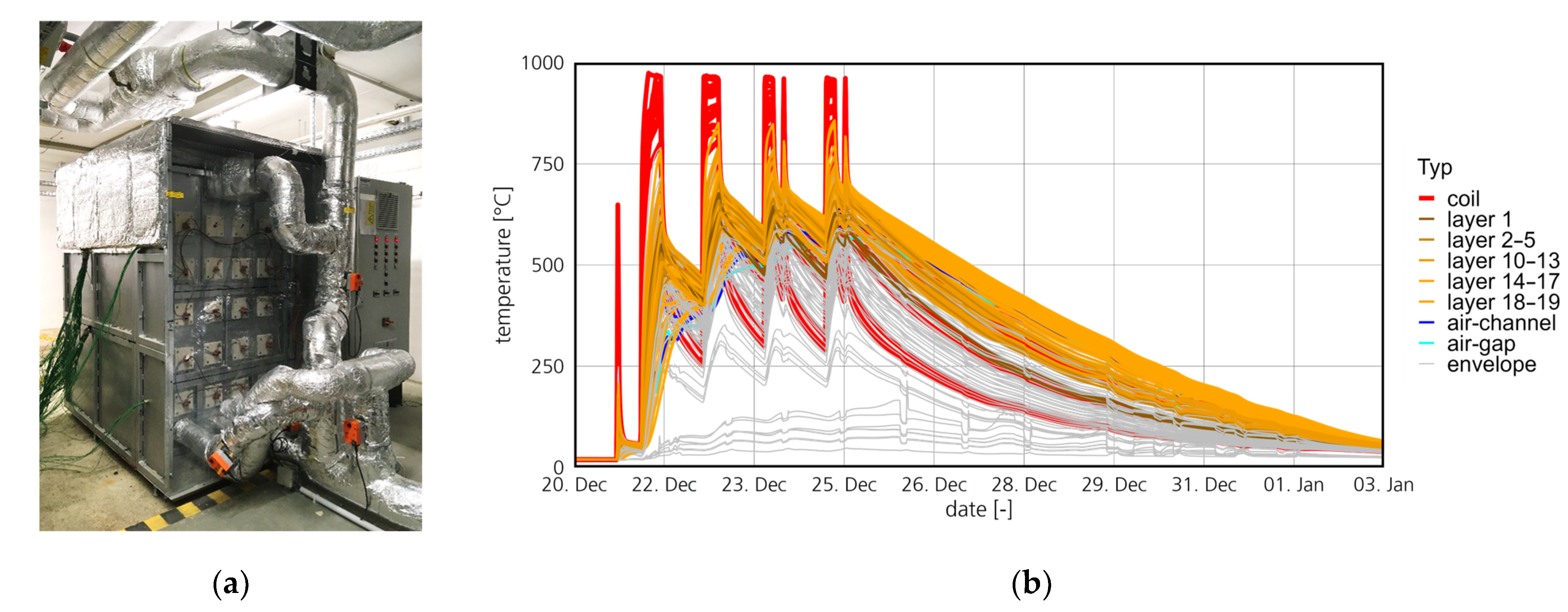
Since the pretest of the high temperature stone storage (HTSS) was conducted on a single heating rod mockup, this setup is not suitable to generate validation data. Therefore, a data period from the final, full-size, HTSS prototype shown in Figure 5a is presented here. The prototype was equipped with about 500 thermocouples to record the heat distribution over the charging periods when the 18 heating coils (1000 °C) heated the stone core up to 800 °C. For the validation, a long heat up period was chosen, and the measured temperature profiles are logged in Figure 5b.
4. Simulation Model Development
To represent the described thermal storage systems and their interactions with the building, a simulation framework is used and further developed. The sketch of the different simulation models working together and described below is drawn in Figure 6.
4.1. Building Simulation Model
To evaluate and optimize but also to design and give dimensions to the buildings equipped with the described systems, a building simulation model was necessary. The hygrothermal building simulation software WUFI® Plus [29,30], developed at the Fraunhofer Institute for Building Physics, IBP, was used to calculate the energy demand and indoor climate. Based on the energy and moisture balance in enclosed spaces (thermal zones), the indoor air temperature and humidity were calculated. Heat and moisture exchange with opaque building components was based on a one-dimensional coupled heat and moisture transport calculation model [31]. Heat gains and losses through windows could be calculated using a simplified or a more detailed model [32]. Desired setpoints in zones are obtained by controlled heat and moisture input from active systems (HVACs). Since the underlying equations were nonlinear, the calculation of indoor air parameters, which in turn become the boundary condition for the assemblies, was performed iteratively. To account for thermal bridges and for the ground heat coupling of basement assemblies, a module for the calculation of two- or three-dimensional heat flow was implemented and validated [33]. Since boundary conditions for 3D objects are defined the same way as for the thermal building envelope (outer or indoor climate), these elements were fully, thermally integrated with the building, i.e., the heat exchange on inner surfaces was part of the zone heat balance.
The WUFI® Plus software was used as the main tool for verification calculations. Some elements such as zoning or 3D objects are inherent features of this tool. To integrate new models, which are not included in the software, specific algorithms can be developed, coded, and attached as plug-ins into the simulation. The main building simulation and plug-in calculation ran in parallel. They were coupled, based on the current state in terms of physical phenomena (current flows, balances, air parameters, etc.) via an iteration scheme that considered all impacting parameters (e.g., heat and/or moisture sources). This can also change the time step, alter the solving method (implicit or explicit), or adapt convergence criteria in particular time steps.
As all measurements were performed in field tests, the environmental conditions could be used as boundary conditions for the TABS and other elements. Thus, the temperature and relative humidity in zones were not calculated, but the measured values were provided as the boundary conditions. The active systems were modeled separately and combined with the building zones and assemblies using plug-in techniques.
4.2. Three-Dimensional Heat Flow Components (3D objects)
If heat flow in a building element cannot be regarded as being one-dimensional, a three-dimensional component model, the 3D object, can be used. Using the WUFI® Plus software, transient three-dimensional heat flow was solved using the finite volume method [34]. The heat-conducting component was first divided into x, y, and z directions, and material data were assigned to the different compounds. The boundary conditions were either defined by local space conditions or as being adiabatic, which allowed us to use the symmetry and reduce the number of numerical grid elements. The software generated variable discretization with denser subdivision at the edge and at the junction of areas with different materials. Instead of one solid material, there were air cavities inside some building components. The elements defined as air-type materials were grouped into one space and balanced like a heat zone. Implicit or explicit solving methods were applied to obtain the transient temperature distributions. The implemented 3D objects were validated according to DIN EN ISO 10211 [35].
Existing 3D objects were adopted for the simulation of the thermal performance of the HTSS and TABS storage. Electric resistance heating rods or piping filled with circulating hot water, described in the following chapter, were regarded as a heat source or sink in the adjacent finite volumes of the 3D object.
4.3. Active Subsystem Models
The 3D object in the simulation framework needs to include the active parts of the storage system. The active system elements were calculated separately but coupled with the inputs and outputs of the building model itself. The coupled values were indoor climate information, setpoint temperatures, heat flows between the active system and the rooms or the 3D object of the storage, and detailed finite volumes with all implemented pipes. The finite volumes sent the temperatures as boundary conditions to the TABS model and, conversely, the TABS model sent the heat source or sink to the finite volumes of the 3D object for each calculated time step.
The detailed calculation models for the active parts of the systems, such as pipes and air channels including their junctions and valves, water tanks, heat exchangers, and heating elements, including their control algorithms, were supplemented to the whole building model via a plug-in and are described below. Some of these sub-models for the active parts were derived from earlier projects [36,37].
4.3.1. Stratified Water Tank Model
The model of the stratified storage tank from [38] was used as buffer storage (TABS storage) as well as the water storage for the WBTS. The model used up to two internal heat exchangers for indirect charging and discharging. The heat exchangers were considered with constant heat transfer coefficients and were adjustable in their connection heights and thus the directly influenced area in the storage tank. The medium in the heat exchanger has constant properties and is simplified as being massless; thus, it does not consider inertia. In addition, there are two double ports for direct loading and unloading. For these, the connection of the tap can be influenced in its height. Three temperature sensors were integrated in the storage tank model, which were adjustable in their mounting height. It was a stratified storage tank with any number of discretized temperature layers, which were isothermal in the horizontal plane. The default value was five layers. The modeling of the storage included heat flows between adjacent layers due to mass movements, as well as due to heat conduction processes in the fluid, along the storage wall and the storage internals.
4.3.2. Pipe Model
The partial model for representing the pipes in the TABS storage and the air channels within the HTSS is described in [39]. It calculates the emitted or absorbed heat flow via heat conduction through a pipe, or an air channel, depending on the temperature conditions between the flowing medium and the surrounding material (y direction in Figure 7). The pipe itself is also discretized by length into several segments, to represent and calculate the flowing medium and its temperature profile (x direction in Figure 7).
Equation (1) was used to calculate the heat flows per segments from the flowing medium to the pipe and further to the material, but also the heat flows along the length of the pipe for the material, pipe, and flowing medium itself. The in the equation is the heat flow in [W]. Furthermore, is the thermal transmittance in [W/(m2K)], is the heat exchanging area in [m2], and is the temperature difference [K] between two segments (x direction), or between the material, pipe, and medium (y direction).
For the pipe and also for the medium, a cylindrical geometry was assumed. Thus, the heat transfer capacities [W/K] of the medium to the pipe were calculated according to Equation (2).
is the heat transfer coefficient in [W/(m2K)] of the flowing medium, is the pipe wall thickness [m], is the thermal conductivity of the pipe wall [W/(mK)], is the pipe segment length in [m], and is the inner pipe diameter [m]. In total, three equations from fluid to material and three from segment to segment were established for each segment. These equations were solved using the Runge–Kutta method of fourth order.
The surrounding in this case was the 3D object and its pipe touching finite volumes. The location of piping in the 3D object was set by its Cartesian coordinate system. A pipe is defined with its starting coordinate as well as its pipe length and direction. In summary, each pipe obtains the inlet temperature, calculates the temperature distribution in the flowing medium and pipe, and computes the heat exchange with the surrounding material per segment and the outlet temperature. The pressure drops within the pipe as well as the friction of the flowing medium were neglected.
4.3.3. Electric Heating Elements
The model of the electric heating elements used the same coupling as the 3D object. The initial position, length, and direction in the coordinate system were also defined. The maximum possible electrical power is an input parameter. The decrease in the heat output with rising temperature, among other things, was also control-related, since the heating rods were partially switched together when the maximum temperature was reached at one point. This was calculated by the empirically derived Equation (3), according to measurements in the HTSS.
is the heat flow of the 3D object in [W], is the available heating power, is the average temperature of all adjacent finite volumes of the 3D object in [°C], and is the temperature in [°C], where the decrease in the heat output starts to be reduced.
4.3.4. Heat Pump
TABS storage requires a heat pump for domestic hot water preparation, which raises the storage temperature on the primary side to the domestic hot water setpoint temperature on the secondary side. As with the domestic hot water heat exchanger in the HTSS system, the required heat demand for domestic hot water in [W] is known (Equation (4)). To simplify, the seasonal energy performance [-] was used to determine the proportion of heat required from the storage tank and the heat pump demand , both in [W]. The maximum temperature differential [-] available on the primary side was calculated (Equation (5)) using the inlet temperature [°C] and the minimum accepted outlet temperature in [°C], on the primary side, in order not to undercool the components too much. The temperature difference in [°C] covering the demand was calculated by Equation (6) with the heat from the storage and the mass flow on the primary side in [kg/s] of the heat pump, as well as the specific heat capacity of water in [J/(kg∙K)].
If the demand temperature difference is smaller than the available temperature difference (), the heat quantity of the storage tank is sufficient. The current return temperature in [°C] is obtained according to Equation (7).
If the heat quantity from the storage tank is no longer sufficient to cover the demand, then the buffer storage tank is reheated electrically to the domestic hot water target temperature.
4.3.5. Heat Exchangers
To calculate the air-to-water heat exchanger, a simplified model using the heat demand for domestic hot water preparation in [W], with respect to the ideal energy balance, was used. The heat demand can be calculated with the hot water tap flow rate in [kg/s], tap setpoint temperature [°C], and temperature of the cold fresh water inlet, in [°C]; see Equation (8). The maximum amount of heat available was calculated by Equation (9), using the mass flow rate in the ventilation duct in [kg/s] and its known inlet temperature in [°C] at the heat exchanger, as well as the same tap setpoint temperature as used before.
The efficiency of the heat exchanger [-] for a non-ideal heat exchanger is introduced. If the available heat quantity is greater than the heat demand for domestic hot water, the demand is taken and the air temperature at the outlet of the heat exchanger is calculated using Equation (10).
If the amount of heat from the system is not sufficient, the maximum possible amount of heat is taken from the system and the remaining energy demand is calculated.
The model to calculate the air-to-air heat exchanger also represents the ideal energy balance and the temperature difference. Since the heat exchanged is not known, this ideal heat exchanger was determined by two flows, defined by their mass flow and the specific capacity of the flowing medium. Thus, the maximum transferable heat quantity could be calculated with both mass flow rates and , both in [kg/s], and two known inlet temperatures, at the warm side of an air circuit [°C] and at the cold side of the other air circuit [°C]; see Equation (11). The specific heat capacity of both flowing mediums, in the warm and in the cold stream, both in [J/(kgK)], might vary according to the flowing medium. The resulting maximum transferable heat quantity was further reduced by the efficiency of the heat exchanger .
In addition, the necessary amount of heat to maintain the setpoint room temperature was known from the building model at each time step. If the maximum amount of heat available is more than the demand from the building [W], space heating from the storage is possible. The outlet temperatures at the heat exchanger, and , both in [°C], were calculated using Equation (12). If the available heat quantity is smaller, or the outlet temperature to the building [°C] is smaller than the setpoint room temperature [°C], the supply air must be reheated to setpoint room temperature. The missing heat quantity is the residual power requirement for reheating.
4.3.6. Pipe Distributor and Collector
In such a flow system, there are two ways to connect the individual subsystems. They can be connected in series, which means that the outlet of one subsystem is connected to the inlet of another sub-model. However, it is also necessary to connect the sub-models in parallel, to have a model for the distribution and merging of flow paths. For example, an air stream is distributed to several air channels when it enters the HTSS and is reunited when it exits. The same occurs in the TABS storage with the piping in the different components.
The flow path distributor connects a single inlet to multiple outlets. Each outlet temperature is equal to the inlet temperature. In total, all outlet mass flow rates must be equal to the inlet mass flow rate. However, a single outlet mass flow rate depends on the setpoint mass flow rate of the open flow path. At first, the model for the pipe distributer calculates the required total setpoint mass flow rate according to all setpoint mass flow rates and the current state (open or closed) in each path. Whenever the inlet mass flow rate at the distributer is not equal to the required total mass flow rate of each opened flow path, a weighting factor is determined. The weighting factor is calculated by the setpoint mass flow rate divided by the required total mass flow rate. Thus, the mass flow rate on each outlet path is the current inlet mass flow rate multiplied by the weighting factor.
The model for merging different flow paths connects multiple inlets to a single outlet. The mass flow rate on the outlet is the total of all inlet mass flow rates. The resulting outlet temperature was calculated by the temperature on each inlet, weighted by its fraction on the total outlet mass flow rate.
4.4. Model Coupling and Sequence of Simulation
To reduce the calculation time and to flexibly link all of the system device models, the simulation methodology of the heating system models, initially developed in [37,40], was further enhanced. To be more flexible and to couple the different system devices of the active system, the simulation was not designed as a whole system. Partial models were solved with their equations at once iteratively. The individual partial or sub-models were coupled in a waterfall model and calculated using an explicit solving technique with very small time steps, normally set to one second. The explicit method used to calculate the active parts of the system is based on a real pipe network of hydraulic or air-carrying systems. Each sub-model is calculated one after the other, coupled with input and output ports with information about temperature and mass flow of the flowing medium. At the beginning of a time step, boundary conditions, such as the room temperatures of the building model, the surrounding temperatures of the pipes, and the air channels from the 3D object, are communicated to the active system model. A sub-model then starts the calculation with initialization values or the input value of the previous time step and calculates the change in the flowing medium at its output, which is again coupled to the input of a subsequent sub-model. In the same way, the following models are calculated. When the last sub-model is calculated, a time step is completed and the calculated values, mainly the heat flows, are returned to the 3D objects as heat sources/sinks and to the building model. For simplification, the pressure drop in the system is neglected.
4.5. Combined Thermal Storage Models
4.5.1. Hot Water Storage Model
The overall simulation of the hot water storage system is performed via the coupled whole system model written in the multi-domain modeling language Modelica via FMI, as described in [41].
4.5.2. TABS Storage Model
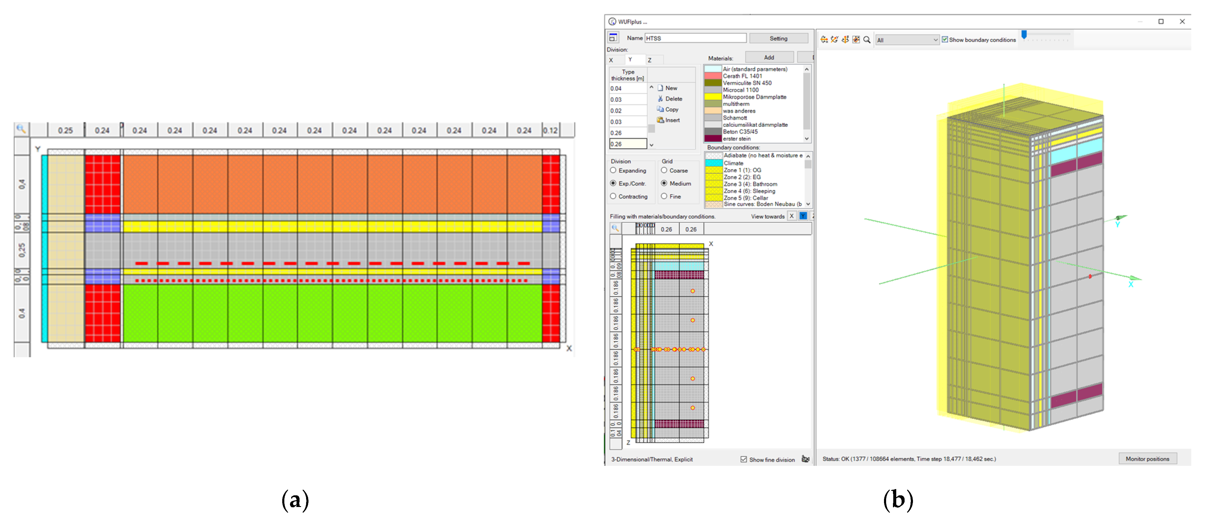
As described above, the 3D object was used to model the inner ceilings and partition walls which were activated in the simulation model. The three-dimensional model can be reduced to two dimensions to improve computation time with reasonable loss in accuracy. The cross-section of a ceiling is shown in Figure 8a. The red dashed line indicates the position of the pipes for heat charging, and the dotted line indicates the position of the active discharge (panel heating) pipes, calculated with the plug-in. On the left side of Figure 8a, the outdoor climate is set as the boundary condition (light blue), followed by some insulation (brown) and bricks (red) for the exterior wall. In between, there is a massive concrete slab (gray, 25 cm thickness in this case). Below the concrete ceiling there is the internal insulation layer (4 cm) and another concrete layer used for panel heating. Above the ceiling, there is a footstep sound insulation covered by a floor screed. The green and orange colors are the coupled zones of the building model below and above the ceiling. Besides the pipes, there are more active system parts involved to represent the thermal storage system. There are partial models for a water tank (for the hydraulic separator and the domestic hot water tank), direct electric-flow-type module water heater, heat pump, pipe junctions, and valves, as well as their control algorithms. The pipe junctions are important to split and merge the mass-flow for the different components, the different activated inner ceilings, and the walls in the building. The panel heating is controlled by the adjoined room’s zone temperature. An additional connection pipework is neglected in the simulation model.
4.5.3. HTSS Model
The HTSS was added as a 3D object to the building simulation. Via defined enclosing surfaces of the 3D object, this exchanges heat with a defined zone of the building model, and passive heat losses are thus modeled. The active part of the HTSS system is calculated via the plug-in and coupled with the 3D object. The plug-in contains calculation models of electric heating elements, ventilation ducts, air–water heat exchangers for domestic hot water production, and air–air heat exchangers for space heating, as well as pipe distributors and valves for air flow control.
The above-described pipe model was used to represent the air channels within the high-temperature stone storage. Instead of water, air with air properties was used as the flowing medium. Because of the air’s low thermal capacity, the time step size for the pipe model was reduced to 0.1 s. Furthermore, partial models were set for the air-to-water and the air-to-air heat exchanger, as well as the water tank model for the domestic hot water. The air channels were coupled to the 3D object (Figure 8b) and ran from the bottom to the top of the hot stone in the middle (gray color). The secondary air path on the outside of the core insulation (small light-blue-colored layer), to keep the passive heat loss of the stone controlled, was also calculated using the air channel pipe model. The heating rods were placed horizontally on different heights of the stone. Because of the symmetric footprint of the HTSS, only a quarter was modeled, as shown in Figure 8b, with the resulting heat fluxes and passive heat losses multiplied by four to account for the whole stone in the building model.
5. Model Validation
Besides the graphical comparison, the following statistical indices are considered to validate the simulation models: NMBE—normalized mean bias error—represents the average deviation between the measurement and the simulation results (tolerance range: +/−10%). CV(RMSE)—coefficient of variation of the root mean square error—shows the variations between the simulation and the measured values (tolerance range: +/−30%). R2—coefficient of determination—shows how close the simulated values are to the values of a regression line of the measured values (tolerance range: >0.75). The applied tolerance ranges are defined according to [42].
5.1. TABS Storage Validation
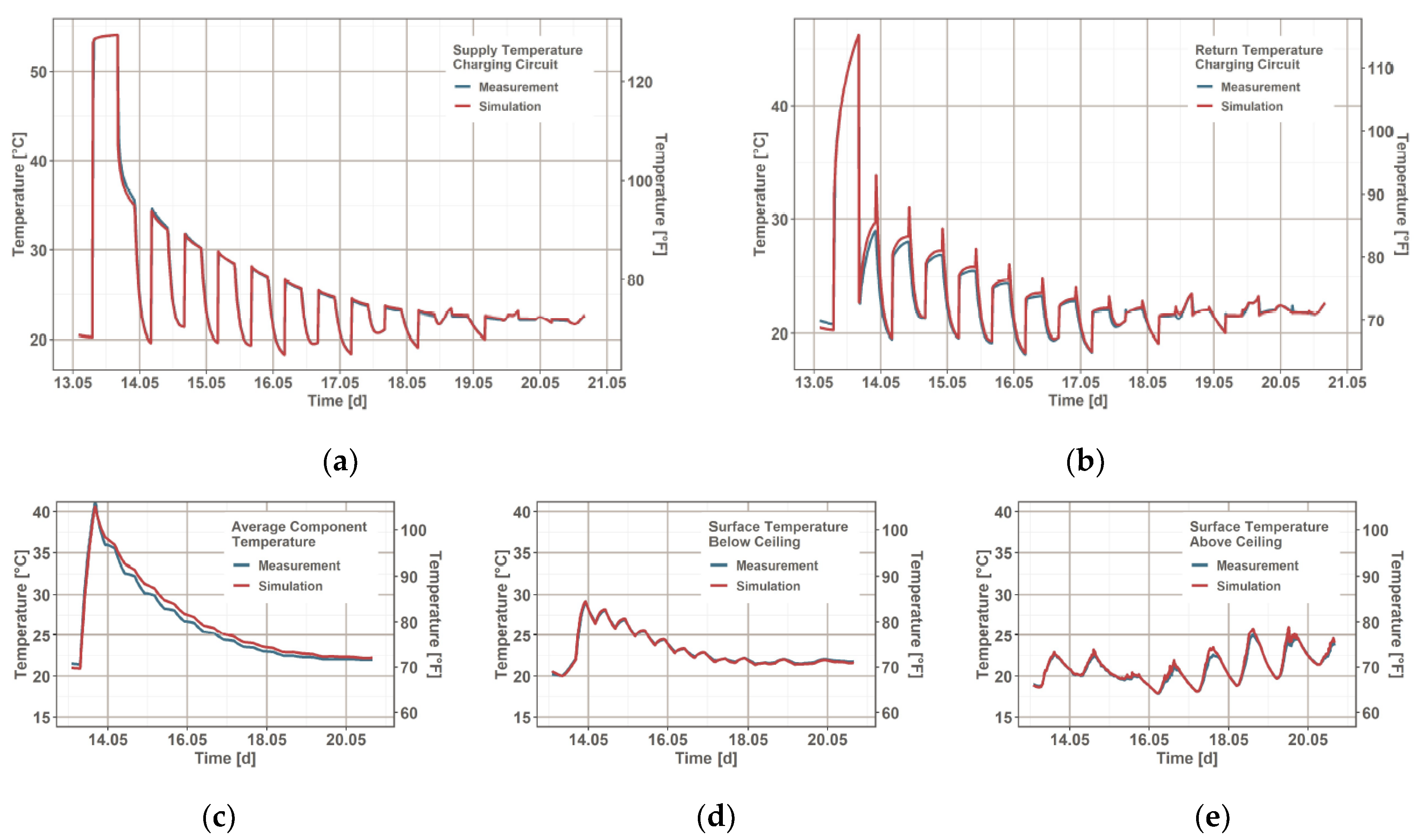
Various sample sequences or operating sequences were investigated on the two ceiling systems, the new construction ceiling and the renovation ceiling. The shown validation is the sequence of charging the storage followed by alternating the discharge, with the active panel heating on and off.
In order to validate the simulation model, the experimental setup was prepared as with the model in the simulation environment. The boundary conditions obtained by the measurements were used as the boundary conditions for the simulation model. These included the ambient temperatures of the air above and below the ceiling and all surface temperatures of the surrounding area, but also the temperature and mass flow of the water in the pipes during the loading. The heat generator was not represented in this validation. After the loading, all of the temperatures of the investigated components, such as surface temperatures and inside temperatures of the ceiling, as well as water temperatures on inlets and outlets and in between, were calculated to be compared to the measured values.
The comparison of the measured values with the calculated results of the simulation shows small differences, but in the expected range. The graphical comparison is presented in Figure 9, and the calculated statistical values are named in Table 2. Among other things, the deviations are due to the degree of detail in the simulation model (homogeneous component layers and material properties, ideal position of the TABS-piping, completely mixed zone air, coarse discretization, etc.) and measurement uncertainties. The temperatures and their statistical indices show good agreement and thus the simulation models are suitable for further investigations, as well as on the entire building.
5.2. HTSS Validation
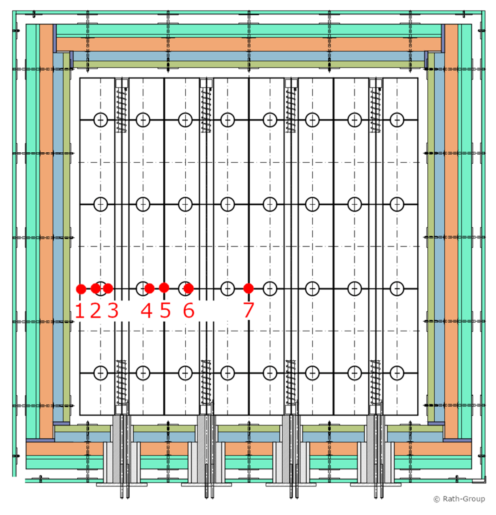
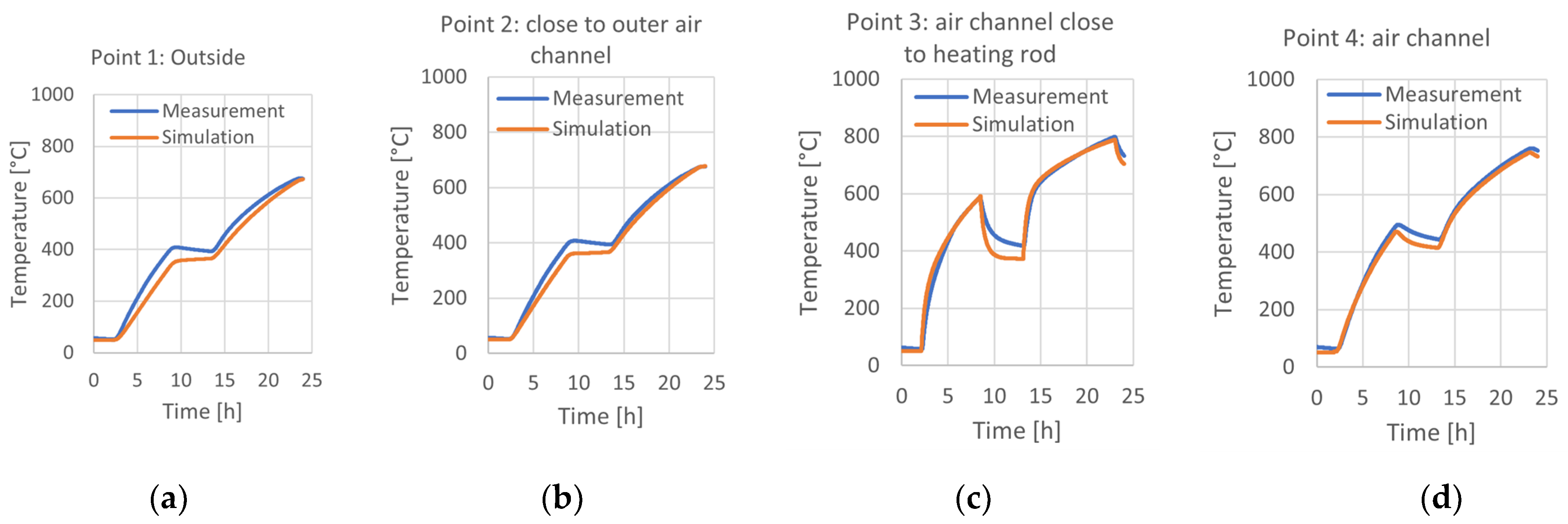
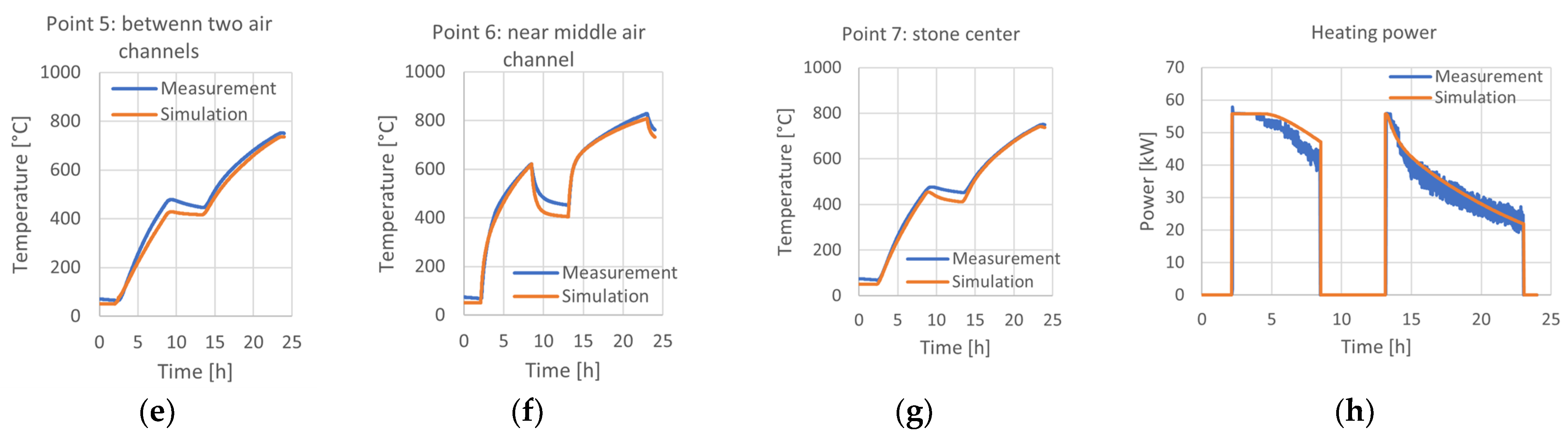
The model representing the HTSS system in the simulation framework was compared with data obtained by the field tests. This paper compares the temperatures at approximately the center of the HTSS, as marked in Figure 10. Graphically, the measured data are compared to the simulation data in Figure 11. The NMBEs for the individual measurement points from number 1 to 7 are as follows: −8.7%; −5.9%; −1.2%; −3.3%; −6.2%; −3.3%; and −3.65%, and for the electrical power it is 5.84%. All of these NMBEs are within the defined tolerance range of +/−10%. In the measurement, the temperature was mostly slightly higher than in the simulation, with slightly lower power introduced. This indicates a higher storage capacity of the simulation model. The ventilation ducts and electric heating elements are correctly considered in the system engineering with the corresponding cross-sectional area and their volume, respectively, but this volume is not deducted in the thermal three-dimensional model in favor of the simplified modeling and considerable reduction in the calculation time.
In addition to comparing the measured data, the model of the HTSS system was tested for plausibility and energy conservation. Basically, the storage can only release as much energy as it has previously absorbed. Figure 12 shows the simulated heat flows of the HTSS. The amount of heat initially introduced during charging is released over the course via the core air (active), purge air, and the outer surface (passive) heat release, so the conservation of energy is respected.
6. Discussion
The level of detail is adjusted to the acceptable computational effort and simulation time for the design of buildings with the described systems, also considering the necessity of small parametric studies for optimization purposes. With a common computer, the described simulation of a multizone building for one year, including one of the thermal storage systems, takes between 6 and 12 h. Some models are set to a low level of detail to keep the simulation within this time frame. There are models which can gain accuracy via parameters, such as a finer mesh size of the finite volumes, but other models can only gain accuracy by taking more physical phenomena into account, such as the pressure drop in the active sub-models, or the representation of the heat exchanging surface of the heat exchanger. Distribution pipes and air ducts are not represented by the model. Even with a higher level of detail of discretization, a fine instead of a course mesh of 3D objects does not result in a significantly smaller deviation between simulation results and measurements. The differences are at least not only related to the level of detail and the employed physical and empirical models. Differences might also be related to uncertainties in the material properties. For example, the results for the HTSS were obtained using the manufacturer’s material properties of the ceramic brick. Even small changes in thermal conductivity and heat capacity result in recognizable deviations. However, with the introduced simulation environment, it is possible to calculate the system behavior and estimate the part of the energy demand which can be covered by the excess electricity, as well as how much residual energy is needed to keep the inner climate within the design conditions. Furthermore, the thermal comfort can be evaluated which is important to prevent overheating. Besides constructive details, variable system settings, such as the supply temperature of the TABS, are crucial for efficiency.
Relating to the thermal storage concepts, the building connection power must have the capacity to charge the thermal storage in the available time. It is important to meet the sweet point between storage dimensions and excess power usage. A complex charging control system, especially for the TABS storage, is important for reducing the overheating caused by the passive heat dissipation of the storage. During spring and fall, the storage should not be fully charged because of the reduced heating demand during that time and the reduced usability of the passive heat dissipation.
7. Conclusions
In this paper, we presented the development of three thermal storage models for space heating and domestic hot water that aim to exploit the overproduction of electricity in electrical grids with high renewable fractions. These systems were based on the use of large-water-based thermal storage (WBTS), insulated thermally activated building systems (TABS), and high-temperature stone storage (HTSS). Various sub-models were successfully coupled to long-term thermal energy storage systems and integrated into existing building simulation software for the simulation-based assessment of these systems. We discussed the challenges of modeling such sub-systems, the complexity of coupling different sub-models, and the mechanisms to integrate them in a whole building simulation framework. We were able to couple an existing building simulation tool with external dynamic models.
Two technologies, TABS storage and HTSS, were experimentally investigated. The models were successfully verified using measured data from the lab, showing the ability of the models to accurately simulate the thermal storage systems’ behavior and performance. This allows one to investigate the potential of these thermal storage systems on how well they can contribute to reducing the problem of overproduction in electrical grids with a high renewable percentage. Parametric studies, not presented in this article, are in the final report of the project “Windheizung 2.0: Langzeitspeicher” [20]. The parametric studies show the potential of the systems regarding the ratio between excess electricity and residual electricity necessary whenever the stored energy is not enough. Target values to cover about 90% of the heating demand in residential buildings with the excess electricity are doable. The performance ratio depends on the dimension of the storage, especially for the WBTS and HTSS. In the case of the TABS, the storage size is limited by the building geometry and the available inner walls and ceilings. Besides the shown expert simulation tool, a simplified tool has also been developed in the project to help planners to design a “Windheizung 2.0” building (a building exploiting excess wind power for heating) and to keep an eye on the named topics.
Even though the TES systems have been evaluated using field measurements and have been simulated using the presented building simulation framework, their real-world integration in buildings may present additional challenges related to building construction specifics, actual performance of the systems, and the occupants’ behavior. To address these challenges, further simulation-based system optimization will be necessary to enable the generalized and more widespread application of these technologies in practice.
Future studies might also apply combinations of the presented systems or use rainwater storage buried in the ground to gain synergy effects. Slow partial charging with on-site photovoltaics or an improvement in the power management while charging might help to keep the electrical house connection power within a reasonable size or lower the necessary storage capacity.
Author Contributions
Conceptualization, F.A. and M.P.; software, J.R. and M.P.; validation, M.K. and M.P.; supervision, H.K.; project administration, M.K. and H.S. All authors have read and agreed to the published version of the manuscript.
Funding
The project on which this paper is based was funded by the German Federal Ministry for Economic Affairs and Climate Action under the funding code 03ET1612A (project “Windheizung 2.0: LZ-Speicher”). The authors are responsible for the content of this publication.
Data Availability Statement
The data presented in this study are available on request from the corresponding author. The data are not publicly available due to format and description of the data, which require additional explanation or context requiring the extent a separate paper.
Conflicts of Interest
The authors declare no conflict of interest.
References
- Arteconi, A.; Hewitt, N.J.; Polonara, F. State of the art of thermal storage for demand-side management. Appl. Energy 2012, 93, 371–389. [Google Scholar] [CrossRef]
- Brockjan, K.; Maier, L.; Kott, K.; Sewald, N. Datenreport 2021; Chapter 13. p. 432. Available online: https://www.destatis.de/DE/Service/Statistik-Campus/Datenreport/Downloads/datenreport-2021.pdf?__blob=publicationFile (accessed on 27 January 2023).
- Bundesnetzagentur 2020 Bericht über Sicherheit, Zuverlässigkeit und Leistungsfähigkeit der Elektrizitätsversorgungsnetze. pp. 11–14. Available online: https://www.bundesnetzagentur.de/SharedDocs/Downloads/DE/Sachgebiete/Energie/Unternehmen_Institutionen/Versorgungssicherheit/Netzreserve/Bericht_%C2%A751_Abs.4b.pdf?__blob=publicationFile&v=2 (accessed on 27 January 2023).
- IBP-Bericht EER 019/2016/952; Windheizung 2.0—Energiespeicherung und Stromnetzregelung mit hocheffizienten Gebäuden. Projektphase 2015/16. Durchgeführt im Auftrag Bayerisches Landesamt für Umwelt und Ökoenergie-Institut Bayern, Fraunhofer Institute for Building Physics IBP: Holzkirchen, Germany, 2016.
- Rogalev, N.; Rogalev, A.; Kindra, V.; Naumov, V.; Maksimov, I. Comparative Analysis of Energy Storage Methods for Energy Systems and Complexes. Energies 2022, 15, 9541. [Google Scholar] [CrossRef]
- Henry, A.; Prasher, R.; Majumdar, A. Five thermal energy grand challenges for decarbonization. Nat. Energy 2020, 5, 635–637. [Google Scholar] [CrossRef]
- Cabeza, L.F.; Martorell, I.; Miró, L.; Fernández, A.I.; Barreneche, C. 1—Introduction to Thermal Energy Storage (TES) Systems. In Woodhead Publishing Series in Energy, Advances in Thermal Energy Storage Systems; Luisa, F.C., Ed.; Woodhead Publishing: Cambridge, UK, 2015. [Google Scholar] [CrossRef]
- Nazari Sam, M.; Caggiano, A.; Mankel, C.; Koenders, E. A Comparative Study on the Thermal Energy Storage Performance of Bio-Based and Paraffin-Based PCMs Using DSC Procedures. Materials 2020, 13, 1705. [Google Scholar] [CrossRef] [Green Version]
- Nghana, B.; Tariku, F. Phase change material’s (PCM) impacts on the energy performance and thermal comfort of buildings in a mild climate. Build. Environ. 2016, 99, 221–238. [Google Scholar] [CrossRef]
- Bruno, F. Using Phase Change Materials (Pcms) for space heating and cooling in buildings. In Proceedings of the AIRAH Performance Enhanced Buildings Environmentally Sustainable Design Conference, Frankfurt, Germany, 19–24 April 2004; pp. 26–31. [Google Scholar]
- Lizana, J.; Chacartegui, R.; Barrios-Padura, A.; Valverde, J.M. Advances in thermal energy storage materials and their applications towards zero energy buildings: A critical review. Appl. Energy 2017, 203, 219–239. [Google Scholar] [CrossRef]
- Ermel, C.; Bianchi, M.; Schneider, P. Energy Model to Evaluate Thermal Energy Storage Integrated with Air Source Heat Pumps. In Proceedings of the Thermal Performance of the Exterior Envelopes of Whole Buildings XV International Conference, Clearwater, FL, USA, 2–5 December 2022. [Google Scholar]
- Xu, J.; Wang, R.Z.; Li, Y. A review of available technologies for seasonal thermal energy storage. Sol. Energy 2014, 103, 610–638. [Google Scholar] [CrossRef]
- Lanahan, M.; Tabares-Velasco, P.C. Seasonal Thermal-Energy Storage: A Critical Review on BTES Systems, Modeling, and System Design for Higher System Efficiency. Energies 2017, 10, 743. [Google Scholar] [CrossRef] [Green Version]
- Sadeghi, G. Energy storage on demand: Thermal energy storage development, materials, design, and integration challenges. Energy Storage Mater. 2022, 46, 192–222. [Google Scholar] [CrossRef]
- Alva, G.; Lin, Y.; Fang, G. An overview of thermal energy storage systems. Energy 2018, 144, 341–378. [Google Scholar] [CrossRef]
- Belz, K.; Kuznik, F.; Werner, K.F.; Schmidt, T.; Ruck, W.K.L. 17—Thermal energy storage systems for heating and hot water in residential buildings. In Woodhead Publishing Series in Energy, Advances in Thermal Energy Storage Systems; Luisa, F.C., Ed.; Woodhead Publishing: Cambridge, UK, 2015; pp. 441–465. [Google Scholar] [CrossRef]
- Schill, W.P.; Zerrahn, A. Flexible electricity use for heating in markets with renewable energy. Appl. Energy 2020, 266, 114571. [Google Scholar] [CrossRef]
- Darby, S.J. Smart electric storage heating and potential for residential demand response. Energy Effic. 2018, 11, 67–77. [Google Scholar] [CrossRef]
- IBP-Abschlussbericht EER 002/2023/720; Thermische Energiespeicher: Windheizung 2.0: Entwicklung von zentralen Hochtemperatur- und Bauteil-Langzeit-Speichern für Windheizung 2.0 Wohngebäude. Durchgeführt im Auftrag PTJ Forschungszentrum Jülich; Fraunhofer Institute for Building Physics IBP: Holzkirchen, Germany, 2023.
- Pazold, M.; Radon, J.; Antretter, F.; Kersken, M.; Sinnesbichler, H. Assessment of Novel Building Integrated Thermal Storage Systems to Enhance Electrical Grid Services in a Heating Dominated Climate. In Proceedings of the Thermal Performance of the Exterior Envelopes of Whole Buildings XV International Conference, Clearwater, FL, USA, 2–5 December 2022. [Google Scholar]
- Antretter, F.; Klingenberg, K.; Pazold, M. All-in-One Design Tool Solution for Passive Houses and Buildings—Monthly Energy Balance and Hygrothermal Simulation. In Proceedings of the Thermal Performance of the Exterior Envelopes of the Whole Buildings XII International Conference, Clearwater, FL, USA, 1–5 December 2013. [Google Scholar]
- Tian, W.; Han, X.; Zuo, W.; Sohn, M.D. Building energy simulation coupled with CFD for indoor environment: A critical review and recent applications. Energy Build. 2018, 165, 184–199. [Google Scholar] [CrossRef]
- Antretter, F.; Pazold, M.; Künzel, H.M.; Sedlbauer, K.P. Anwendung hygrothermischer Gebäudesimulation. In Bauphysik Kalender; Fouad, N.A., Ed.; Wilhelm Ernst & Sohn: Berlin, Germany, 2015. [Google Scholar] [CrossRef]
- SMARD Bundesnetzagentur 2022 Negative Wholesale Prices. Available online: https://www.smard.de/page/en/wiki-article/5884/105426 (accessed on 27 January 2023).
- ZIES-Endbericht 2017 Entwicklung von Steuerungssignalen zur Systemdienlichen und Ökologischen Stromabnahme. Available online: https://zies.hs-duesseldorf.de/forschung-und-entwicklung/energiewirtschaft/projekte/Documents/WH2.0%20-%20Endbericht.pdf (accessed on 27 January 2023).
- Kersken, M.; Strachan, P. Twin House Experiment IEA EBC Annex 71 Validation of Building Energy Simulation Tools—Specifications and Dataset. 2020. Available online: https://fordatis.fraunhofer.de/handle/fordatis/161 (accessed on 27 January 2023). [CrossRef]
- Kersken, M.; Strachan, P.; Mantesi, E.; Flett, G. Whole building validation for simulation programs including synthetic users and heating systems: Experimental design. In Proceedings of the Nordic Symposium on Building Physic, Tallinn, Estonia, 7–9 September 2020. [Google Scholar]
- Holm, A.; Künzel, H.M.; Sedlbauer, K. The hygrothermal behaviour of rooms: Combining thermal building simulation and hygrothermal envelope calculation. In Proceedings of the 8th International IBPSA Conference, Eindhoven, The Netherlands, 11–14 August 2003; pp. 499–504. [Google Scholar]
- Antretter, F.; Sauer, F.; Schöpfer, T.; Holm, A. Validation of a hygrothermal whole building simulation software. In Proceedings of the 12th Conference of the International Building Performance Simulation Association, Sydney, Australia, 14–16 November 2011; pp. 1694–1700. [Google Scholar]
- Künzel, H.M. Simultaneous Heat and Moisture Transport in Building Components. Ph.D. Thesis, University of Stuttgart, Stuttgart, Germany, 1994. Available online: https://www.building-physics.com (accessed on 27 January 2023).
- Radon, J.; Pazold, M.; Antretter, F. A detailed window model for hygrothermal building simulation. In Proceedings of the Thermal Performance of the Exterior Envelopes of Whole Buildings XIV International Conference, Clearwater, FL, USA, 9–12 December 2019. [Google Scholar]
- Antretter, F.; Radon, J.; Pazold, M. Coupling of dynamic thermal bridge and whole-building simulation. In Proceedings of the Thermal Performance of the Exterior Envelopes of Whole Buildings XII International Conference, Clearwater, FL, USA, 1–5 December 2013. [Google Scholar]
- Eymard, R.; Gallouët, T.; Herbin, R. Handbook of Numerical Analysis 7; North-Holland: Amsterdam, The Netherlands, 2000; pp. 713–1018. [Google Scholar]
- DIN EN ISO 10211:2008; Wärmebrücken im Hochbau—Wärmeströme und Oberflächentemperaturen—Detailierte Berechnunge. Deutsches Institut for Normung: Berlin, Germany, 2008.
- Pazold, M.; Antretter, F.; Radon, J. HVAC Models coupled with hygrothermal building simulation software. In Proceedings of the 10th Nordic Symp, Lund, Sweden, 15–19 June 2014; pp. 854–863. [Google Scholar]
- Antretter, F.; Fink, M.; Pazold, M.; Herkel, S.; Ohr, F.; Steiger, S.; Reiß, J. Deutsche Mitarbeit im ECBCS-Annex RAP-RETRO. 2014, pp. 203–204. Available online: https://www.baufachinformation.de/deutsche-mitarbeit-im-ecbcs-annex-rap-retro/bu/2020019005187 (accessed on 27 January 2023).
- Ohr, F. Weiterentwicklung und Validierung Eines Numerischen Warmwasserspeichermodells. Master’s Thesis, Hochschule Esslingen, Esslingen, Germany, 2011. [Google Scholar]
- Jacob, D. Gebäudebetriebsoptimierung—Verbesserungen von Optimierungsmethoden und Optimierung unter Unsicheren Randbedingungen. Ph.D. Thesis, Universität Karlsruhe TH, Karlsruhe, Germany, 2012. [Google Scholar]
- Burhenne, S.; Radon, J.; Pazold, M.; Herkel, S.; Antretter, F. Integration of HVAC Models into a Hygrothermal Whole Building Simulation Tool. In Proceedings of the 12th Conference of International Building Performance Simulation Association, Sydney, Australia, 14–16 November 2011. [Google Scholar]
- Pazold, M.; Burhenne, S.; Radon, J.; Herkel, S.; Antretter, F. Integration of Modelica models into an existing simulation software using FMI for Co-Simulation. In Proceedings of the 9th International MODELICA Conference, Munich, Germany, 3–5 September 2012. [Google Scholar]
- DOE/EE-1287-0286 7300; M&V Guidelines: Measurement and Verification for Performance-Based Contracts Version 4.0. EERE Publication and Product Library: Washington, DC, USA, 2015. Available online: https://www.osti.gov/servlets/purl/1239725 (accessed on 27 January 2023).
Figure 1.
Sketch diagram of the hydraulic concept of the water-based heat storage system with the hot water tank.
Figure 1.
Sketch diagram of the hydraulic concept of the water-based heat storage system with the hot water tank.

Figure 2.
Sketch of the TABS storage to supply a building with space heating and domestic hot water.
Figure 2.
Sketch of the TABS storage to supply a building with space heating and domestic hot water.

Figure 3.
(a) Technical drawing of the HTSS including the stone core made of bricks, the different insulation layers, and air channels. (b) Sketch of the integration of an HTSS into the technical building equipment for supplying a building with space heating and domestic hot water. It shows the operating state with simultaneous hot water preparation and supply air heating (space heating).

Figure 4.
(a) New construction TABS storage in the IBP’s technical center before closing the 4th wall. (b) Retrofit TABS storage system in the twin house’s living room.
Figure 4.
(a) New construction TABS storage in the IBP’s technical center before closing the 4th wall. (b) Retrofit TABS storage system in the twin house’s living room.

Figure 5.
(a) Final, full-size HTSS prototype. (b) Long charging period with the temperatures of the heating rods (coils) (red) and all thermocouples in the stone core (orange) and the envelope (gray).
Figure 5.
(a) Final, full-size HTSS prototype. (b) Long charging period with the temperatures of the heating rods (coils) (red) and all thermocouples in the stone core (orange) and the envelope (gray).

Figure 6.
Sketch of different simulation models working together to build the whole building simulation framework to design and investigate the presented thermal storage systems.
Figure 6.
Sketch of different simulation models working together to build the whole building simulation framework to design and investigate the presented thermal storage systems.

Figure 7.
Scheme cut of pipe model with pipe length in x, and material layers in y direction.

Figure 8.
(a) Two-dimensional geometry representation of a thermally activated ceiling in the simulation software. The red dashed line indicates the position of the inner charging pipes and below the red dotted line indicates the pipes for the ceiling panel heating. (b) Three-dimensional geometry model of the high-temperature stone storage in the simulation software.

Figure 9.
Comparison between measurement and simulation of supply (a) and return (b) temperatures in the TABS in the concrete core of the ceiling. Comparison of component average temperature (c), surface temperature below (d) and above (e) the ceiling, and the 3D object coupled with the TABS model inside.

Figure 10.
Location of measurement points (highlighted in green) for comparison with simulation variables.
Figure 10.
Location of measurement points (highlighted in green) for comparison with simulation variables.

Figure 11.
Graphical comparison of measured data and simulation data of the HTSS system.


Figure 12.
HTSS: simulated thermal energy with full charging and subsequent active and passive heat dissemination for space heating.
Figure 12.
HTSS: simulated thermal energy with full charging and subsequent active and passive heat dissemination for space heating.


Table 1.
Charge and discharge sections of the experimental program of the two units of TABS storage.
Table 1.
Charge and discharge sections of the experimental program of the two units of TABS storage.
| Experimental Section | |||||||||||||||
|---|---|---|---|---|---|---|---|---|---|---|---|---|---|---|---|
| 1 | 2 | 3 | 4 | 5 | 6 | 7 | 8 | 9 | 10 | 11 | 12 | 13 | 14 | 15 | |
| New TABS | 100% | P | 100% | A | 100% | A | 50% | A | 100% | A | 50% | A | R | 100% | Ad |
| Retrofit TABS | 100% | P | 100% | A | 50% | A | 50% | CC | A | 100% | Ad | R | Rc | ||
| Legend: | % | Charge to the named % | CC | Charge from 50% up to 100% | |||||||||||
| P | Passive discharge | R | Reheat, surface only | ||||||||||||
| A | Active discharge | Rc | Reheat, surface only; intermediate cycle | ||||||||||||
| Ad | Active–passive discharge; 6 h intermediate cycle | ||||||||||||||
Table 2.
Statistical indices of comparing the simulation to the temperature measurement of a single example case on the ceiling TABS storage for new buildings.
Table 2.
Statistical indices of comparing the simulation to the temperature measurement of a single example case on the ceiling TABS storage for new buildings.
| Inlet Water | Outlet Water | Average Component | Surface Below | Surface Above | |
|---|---|---|---|---|---|
| NMBE | 1% | 1% | 1% | 0% | 1% |
| CV(RMSE) | 2% | 3% | 1% | 1% | 2% |
| R2 | 0.99 | 0.99 | 1.00 | 1.00 | 0.98 |
Disclaimer/Publisher’s Note: The statements, opinions and data contained in all publications are solely those of the individual author(s) and contributor(s) and not of MDPI and/or the editor(s). MDPI and/or the editor(s) disclaim responsibility for any injury to people or property resulting from any ideas, methods, instructions or products referred to in the content. |
© 2023 by the authors. Licensee MDPI, Basel, Switzerland. This article is an open access article distributed under the terms and conditions of the Creative Commons Attribution (CC BY) license (https://creativecommons.org/licenses/by/4.0/).
Share and Cite
MDPI and ACS Style
Pazold, M.; Radon, J.; Kersken, M.; Künzel, H.; Antretter, F.; Sinnesbichler, H. Development and Verification of Novel Building Integrated Thermal Storage System Models. Energies 2023, 16, 2889. https://doi.org/10.3390/en16062889
AMA Style
Pazold M, Radon J, Kersken M, Künzel H, Antretter F, Sinnesbichler H. Development and Verification of Novel Building Integrated Thermal Storage System Models. Energies. 2023; 16(6):2889. https://doi.org/10.3390/en16062889
Chicago/Turabian StylePazold, Matthias, Jan Radon, Matthias Kersken, Hartwig Künzel, Florian Antretter, and Herbert Sinnesbichler. 2023. "Development and Verification of Novel Building Integrated Thermal Storage System Models" Energies 16, no. 6: 2889. https://doi.org/10.3390/en16062889
Note that from the first issue of 2016, this journal uses article numbers instead of page numbers. See further details here.