1. Introduction
Some wells can naturally produce oil at the start of production by using reservoir primary drive mechanisms such as solution gas drive, gas expansion, and strong water drive. However, most reservoir energies are finite, will deplete over time, and cannot naturally lift hydrocarbons to the surface [
1]. An AL is a production system unit that lifts the hydrocarbons from the reservoir to the surface to support insufficient reservoir energy [
2].
The AL is a milestone in the oil and gas industry since it accounts for 95% of worldwide oil production [
3]. There are several types of AL: sucker rod pumping (SRP) or beam pumping unit (BPU), progressive cavity pump (PCP), gas lift (GL), electrical submersible pump (ESP), plunger lift (PL), hydraulic jet pump (HJP), and hydraulic piston pump (HPP). SRP produces approximately 70% of oil worldwide and is postulated to be the oldest lifting method [
4]. Optimum AL selection is critical since it determines the daily fluid production (daily revenue) that the oil corporations will gain. The AL selection techniques in the literature study the advantages and disadvantages of each lifting method considering field conditions, well, and reservoir parameters [
5,
6]. They use qualitative methods, primarily relying on engineers’ personal experience [
7]. The critical issue is that the field parameters are dependent on and change over production years. In addition, the parameters are neither theoretically nor numerically correlated, leading to inconstancy in the selection and much time spent on analysis. Therefore, more expenses emerge due to AL replacement within a short production period. Some AL experts suggest that old selection techniques have nearly vanished and are, to some extent, outdated [
8].
The uncertainty in field data and screening resulted in different selection methods and a gap in the universal selection criteria. Another gap in the AL selection methods is that the crucial field factors have not been critically identified. There should be one or more factors in each field parameter category (production, operation, economic, or environmental) that predominantly affect the selection in either adequacy or elimination of the nominated AL. This pushed many companies to establish their own selection systems or develop computer programs based on their field conditions [
9,
10,
11].
This research aims to develop a universal AL selection model and examine a new selection criterion based on AL production performance by considering only the field production dataset. Furthermore, the goal is to identify the critical production factors that primarily influence AL selection. This study applied it to select PCP, BPU, GL, ESP, and the ability to flow naturally. The model was also devoted to a wider selection of AL sizes. The project applied supervised ML (via Python), a guided process where inputs and outputs are provided to let the algorithm find relevant patterns between those parameters [
12]. Five algorithms were used to model AL selection: logistic regression (LR), support vector machines (SVM), K nearest neighbors (KNN), decision tree (DT), and random forest (RF). The model determined how successful the process is when applied to only field production data.
2. Materials Preparation
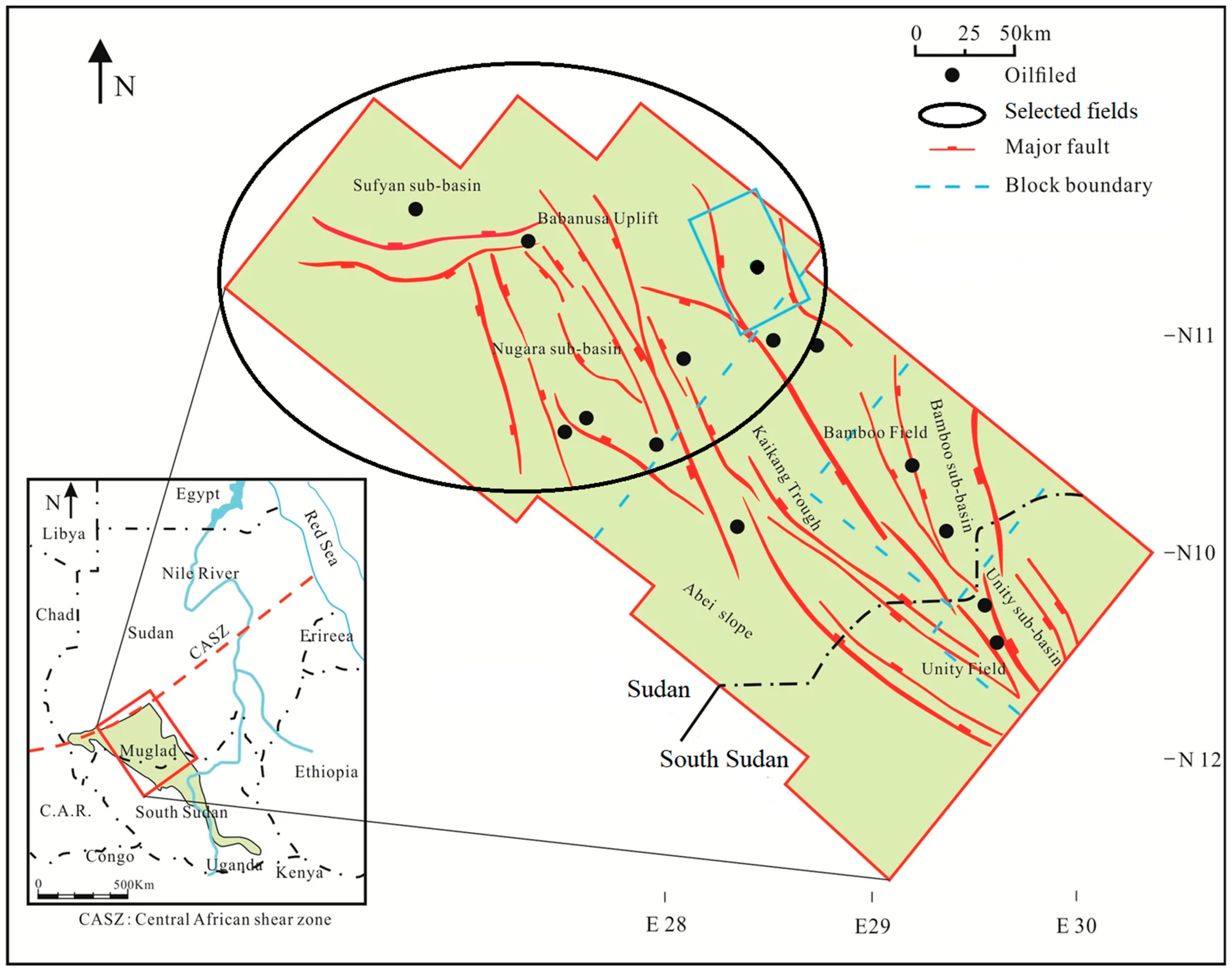
The data contains oil and gas production and recovery methods from 2006 to 2021 for light, medium, heavy, and extra-heavy oil wells. Twenty-four wells were randomly selected as the model dataset. The selected field is in the Muglad basin (
Figure 1 [
13]), has more than 500 oil wells, and comprises seven subfields (blocks) spread over approximately 17,800 square km in seven remote locations [
14,
15].
The reservoir lithology is sandstone interbedded with shale and has three main formations:
(1) A is a deep formation that produces light oil and gas;
(2) B is a shallow formation that produces heavy and extra-heavy oil;
(3) C is a deep formation that produces light oil.
Two more tight formations, D and E, have low oil reserves.
The field’s estimated oil reserve is more than 500 million barrels. Most production wells are completed with 9⅝ inch casing, 2⅞ inch, 3½ inch, and 4½ inch production tubing. Wells’ depths range from 500 m in shallow reservoirs to more than 3000 m in deep reservoirs.
Most light oil wells started production in NF at the beginning of their production lives before moving toward AL. Four primary artificial lift methods are installed: PCP, SRP, GL, and ESP. PCP and SRP have been the primary lifting methods since the field started production in 2003. The implemented recovery methods are water-flooding [water injection (WI)], nitrogen injection (NI), gas injection, and thermal recovery [cyclic steam stimulation (CSS) and steam flooding (SF)]. PCP is installed for cold heavy oil production (CHOP) and cold heavy oil production with sand (CHOPS). BPU and metal-to-metal PCP (MTM_PCP) are used with thermal recovery, while GL and ESP produce light oil.
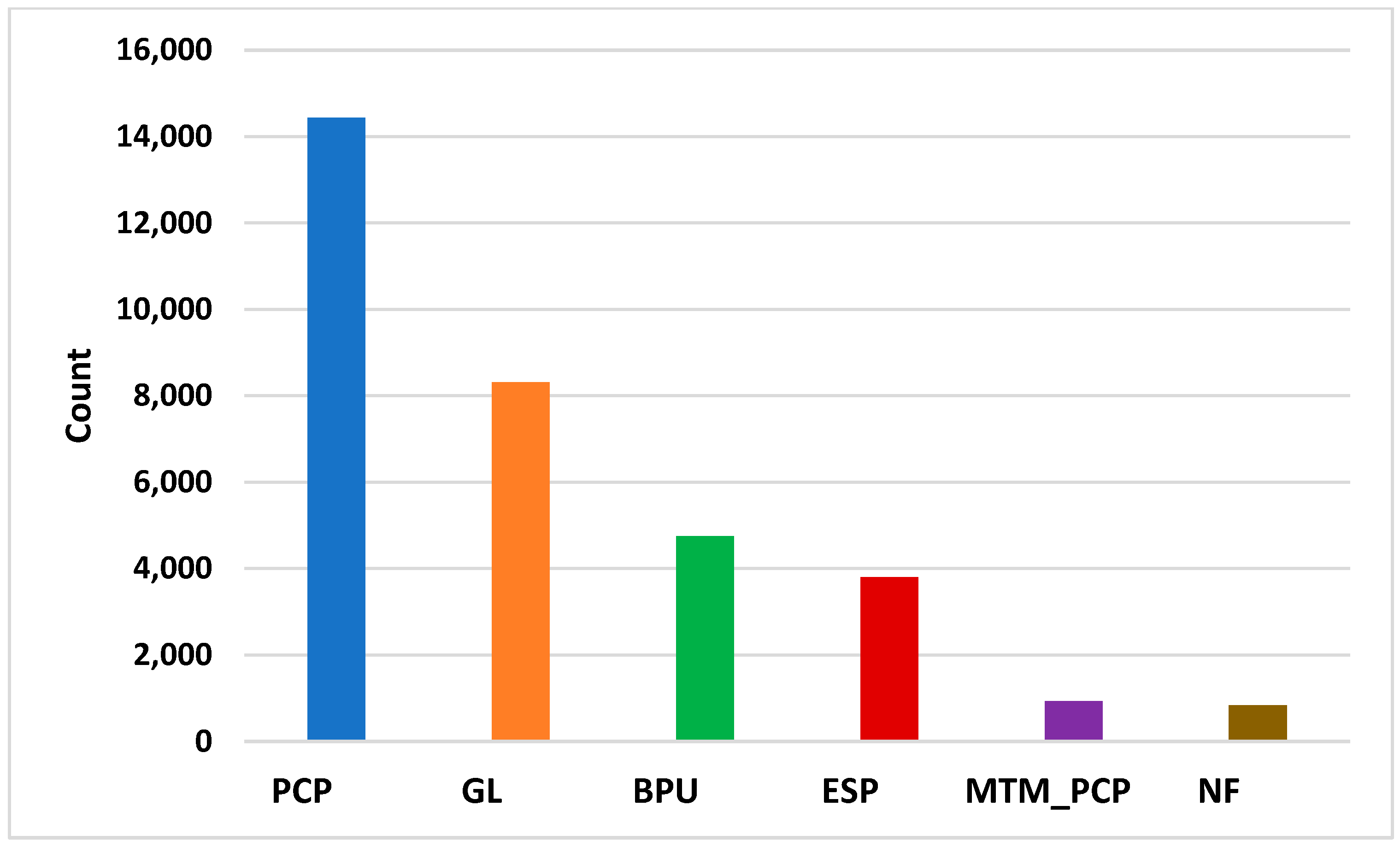
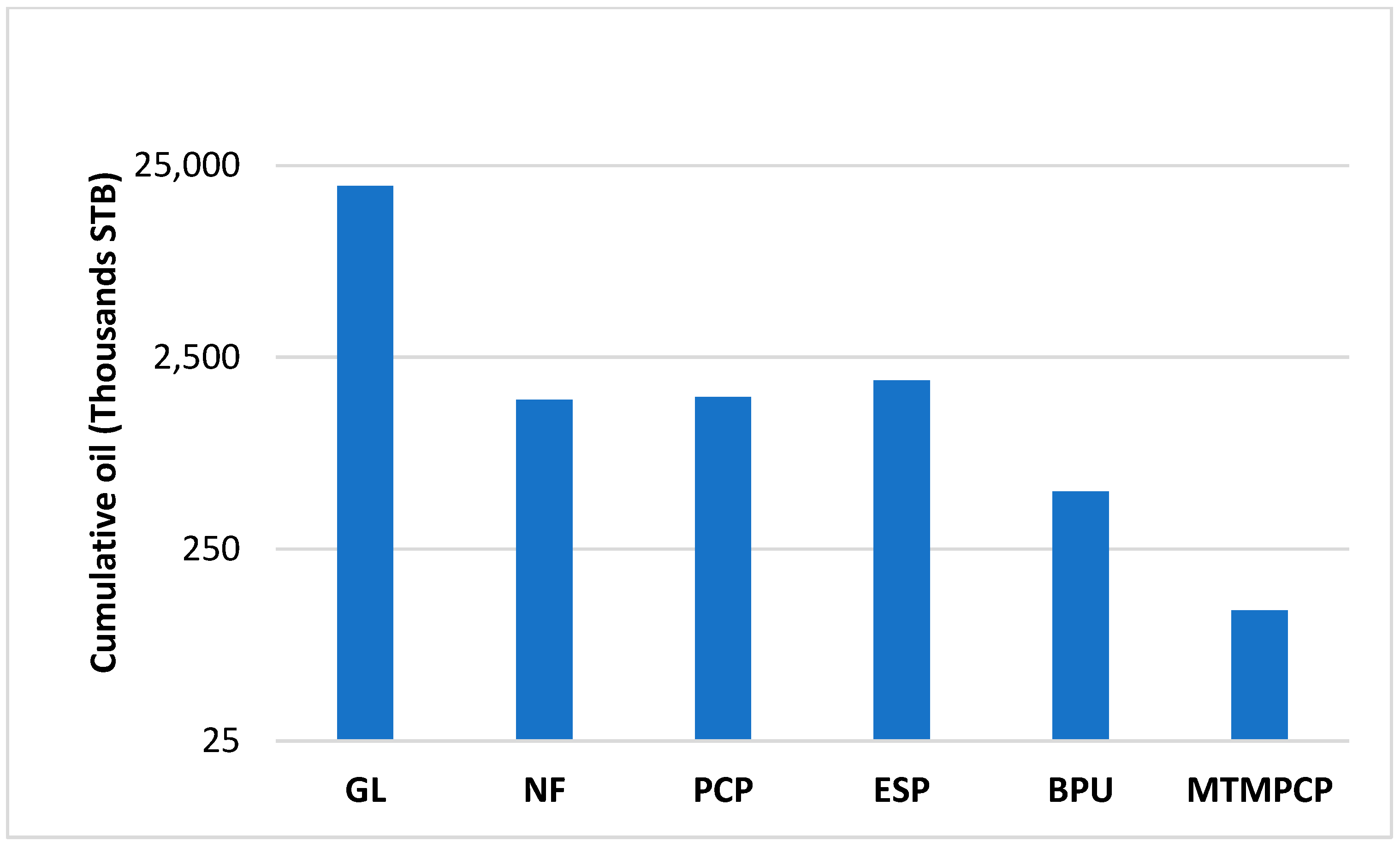
Figure 2 demonstrates the distribution of AL in the dataset. PCP dominates lifting methods in the field, even though the cumulative fluid production by GL is higher than PCP, ESP, and BPU, as shown in
Figure 3. Nonetheless, NF cumulative production is high; it rapidly drops after a short production period because of insufficient reservoir energy. The imbalance in the data may lead to an accuracy paradox if it is not up- or downsampled (this refers to the labels being better when there is approximately equal class distribution in the dataset) [
16]. In our model, the data was kept imbalanced to reflect the actual field state and assess the model’s robustness in AL selection. Some recent studies have shown developments in modeling imbalanced data and learning from it [
17].
3. Methods Application
AL selection is a classification problem since the targeted labels are categorical. The algorithms have been selected accordingly to build the model. The ML algorithms cannot directly perform modeling on raw data, though it is cleaned and pre-processed using data wrangling. Data wrangling is considered the most challenging step for the success of ML [
19]. The process is commonly performed through these steps: data collection, feature selection, data structuring, outlier and duplicate removal, and missing data cleaning. The data wrangling application swept 26,571 outliers and missing values, as well as 4578 duplicates, from the raw dataset. The data was then normalized between 0 and 1 to reduce the generalization error, and the categorical parameters were encoded as the algorithms deal solely with digits.
The modeling was applied to 24 production wells consisting of approximately 465,000 samples after cleaning and preprocessing. Data from 16 wells ranging from 2006 to 2019 was used for model training and validation (approximately 429,000 samples). Two wells minimum were selected from each subfield to ensure the model has a piece of information from each block. The model used 12 wells to train and learn the installed lifting method in each well according to input parameters and field conditions. The remaining four wells in the dataset were used to validate the model. This approach differs slightly from the common train-test-split in ML applications, where the algorithm randomly splits the dataset that is given in bulk. Then the model was tested by a new dataset of eight wells with approximately 11,600 samples ranging from 2020 to 2021. The use of recent data is to test model performance under current and future field production conditions. Moreover, to measure how the model will act on future unlabeled data.
Nominating which ML algorithms to use is critical, as choosing them depends on their accuracy [
20]. It is rare and challenging to use one classifier for classification and find two algorithms with the same accuracy because each algorithm has its own learning approach from data [
12]. The algorithms’ significance is different; thus, combining two or more algorithms is recommended for excellent results [
21,
22]. We selected algorithms that can quickly and efficiently model field data and handle outliers and noise in field parameters. These five algorithms (SVM, LR, KNN, DT, and RF) have been selected for modeling to build a combination of different classifiers for adequate results. The algorithms with the best prediction accuracy on training and validation were then used to predict AL on the test dataset and determine the critical features.
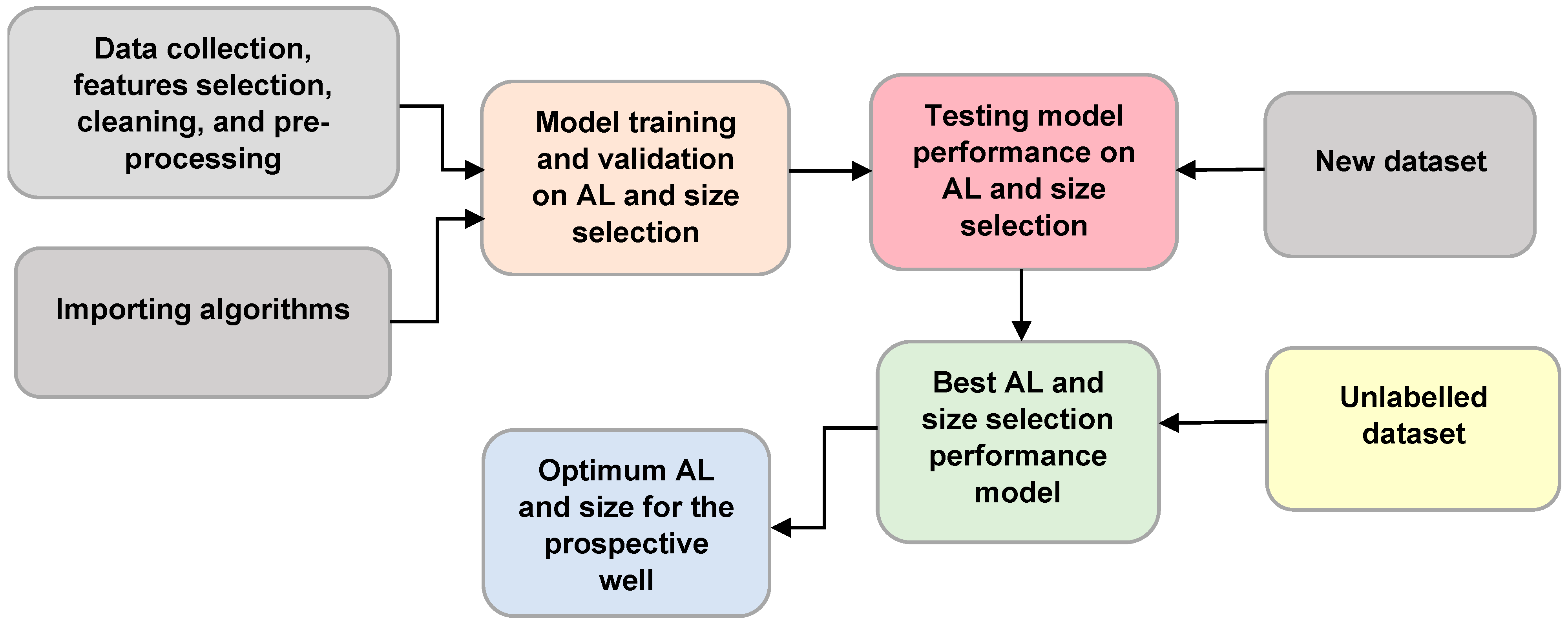
Figure 4 illustrates the simplified workflow of the AL and size selection models.
Ounsakul [
18] demonstrated the process of AL selection (
Y) using ML algorithms as a function of field data
f(X), which is written as:
or
In our model, the equation is written as:
The equation explains that the data quality determines the optimum AL selection. In supervised learning, the data are provided to the algorithms, which are a set of mathematical equations where the inputs X and outputs Y are given. The algorithms train and learn by connecting the input variables to the outputs and exploring each variable’s importance in the dataset. The algorithms then predict the new output (AL) with the best accuracy based on training results.
Algorithms Classification Criteria
- (a)
LR solves the probability P(Y|X) task by learning from a training dataset Dt written as a vector of weights and a bias (
WiXi + b), where the weight
Wi is the importance of the feature
Xi in the dataset. To make a classification on a new test dataset, LR calculates the weighted sum class evidence
z and then passes the result down to the sigmoid function
σ (z), which narrows the results between 1 true and 0 negative class. The algorithm uses the decision boundary of 0.5 to predict the classes [
23].
- (b)
SVM is a binary classifier; however, it can be used for multiclass classification by breaking down the problem into a series of binary classification cases. To do this, we applied the OVO (one vs. one) approach. The concept is that each classifier separates the points of two classes, including all OVO classifiers, to establish a multiclass classifier. The number of classifiers needed for this is calculated using n(n − 1)/2 (n = no of classes). Eventually, the most common class in each binary classification is then selected by voting [
24]. We assume that we have a training dataset Dt {
Xi, Yi} that is binary and linearly separable, where each Xi has dimensionality q and is either one of
Yi = −1 or
Yi = +1 (here q = 2). The training data points can be described as follows:
The SVM draws hyperplanes to separate the classes of each training data point. The hyperplane is expressed as
W ·
X +
b = 0. The support vectors separate the hyperplanes, while the machines keep the distance as far as possible between the hyperplanes that separate the classes. In our multiclassification problem, if the data points are not linearly separable, then the SVM applies the kernel function K(
Xi,
Xj) to recast the data points into a higher-dimensional space
X⟼∅
(X) to be separable [
25]. Thus, the training data points recasting into the higher space are written as:
We applied the radial-based kernel (Gaussian kernel) in our model, which is expressed as:
where
γ controls the width of the kernel function. The decision function of voting that provides the n class label of the
mth function is written as [
24]:
- (c)
In KNN, we have a given training dataset Dt {(X1, Y1), (X2, Y2),…,(Xn, Yn)}, and the algorithm calculates the Euclidean distance of each class to all training data points using the below formula. Then construct a boundary for each class by determining the K’s nearest neighbor.
The algorithm’s performance is susceptible to the K value, which is difficult to estimate. A small K will result in overfitting, while a large K leads to class boundary intersections and training data scattering in many neighborhoods. The best option is to try different K values until the highest accuracy is achieved [
26].
- (d)
The DT consists of a root node, internal nodes, and leaf nodes that assign the class labels. The concept of DT is that it identifies the informative features regarding each class label. To obtain that, we use the CART (classification and regression tree) because some features are categorical as well as the outputs; the DT applies the Gini index in each node to split the data. Gini is defined as a measure of the probability of incorrect predictions when the features are selected randomly [
27]. Assume we have a Dt training dataset; the Gini index is calculated using the following equation:
where
Pi is the probability of partitioned data of class
i in Dt and n is the total number of classes of Dt. The feature with a lower
Gini value is used to split the data.
- (e)
In RF, let Dt be a training dataset {(X
1, Y
1), (X
2, Y
2),…,(Xn, Yn)} since the RF is a combination of trees, the RF applies bagging (bootstrap aggregating), an aggregation of multi-tree results. The idea is that the RF randomly splits the training dataset to bootstrap samples to create multi-trees and repeats the process. The class Y that has the majority among the results of the trees is then selected by voting [
28]. The RF classifies through the following steps [
29]:
Let
be the class prediction of the
bth tree, then the conclusive predicted class is given by:
4. Results and Discussion
4.1. AL Selection Results
The study demonstrates the optimum AL and size selection, as well as the most crucial production factors that affect the selection. The results were validated with the actual lifting methods used in the field, considering that they are the optimum lifting methods according to the previous selection screening and the production performance simulation. The outcomes of this research have provided insight into the robustness of the ML model in AL selection using only production data.
Table 1 summarizes the AL selection model training and validation accuracies scored by each algorithm. The algorithms performed well in training and validation, while the two algorithms, DT and RF, had excellent results on the new test dataset, as shown in
Table 2, including precision, recall, and F1 scores. RF scored 92.42% accuracy, and DT scored 93.02%. Both RF and DT have test accuracy that is approximately equivalent to their validation accuracy. SVM, LR, and KNN testing accuracies are between 58 and 64%.
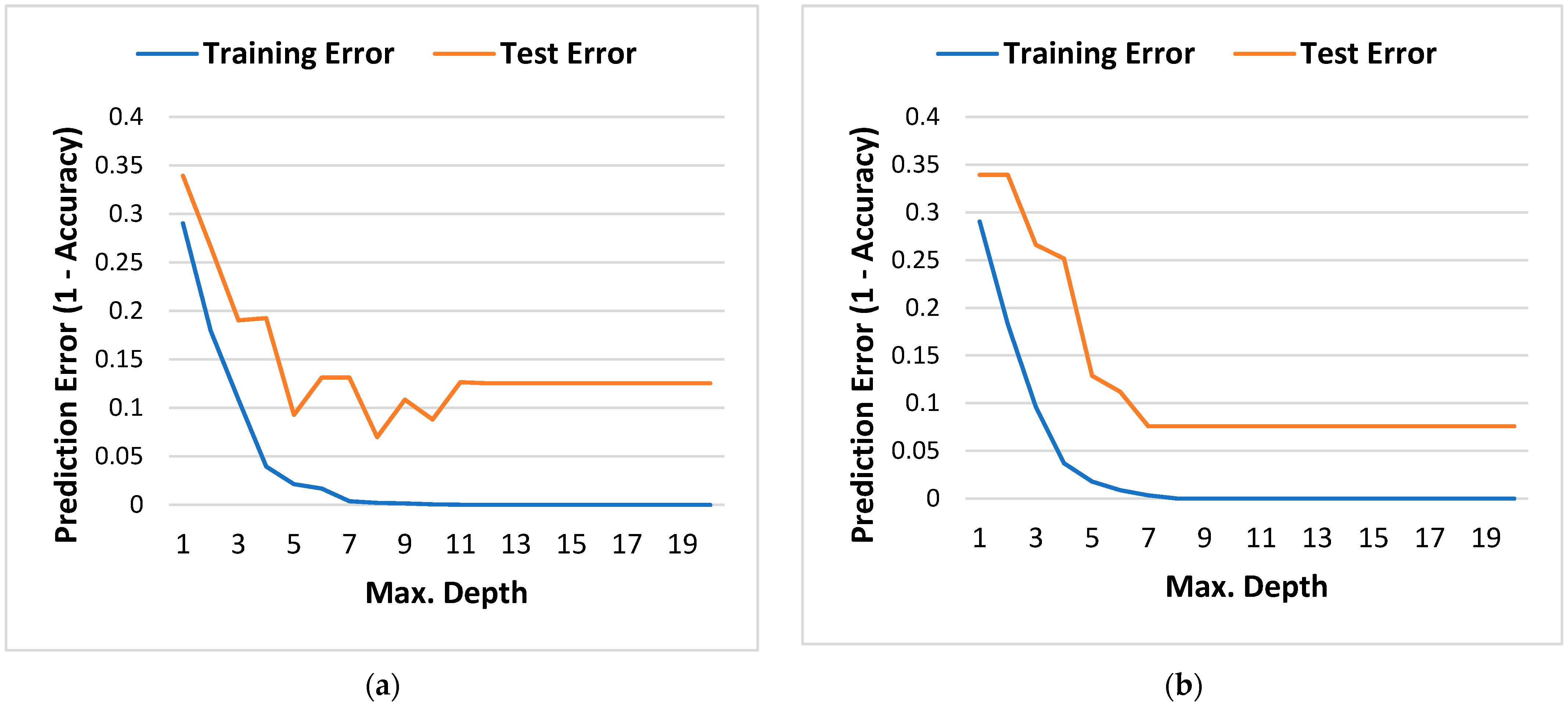
The accuracy of both RF and DT in training and testing is demonstrated in
Figure 5. Both algorithms obtained their highest test accuracy at a maximum tree depth of 7. It is important to note that the obtained accuracy considers data imbalance and actual field conditions.
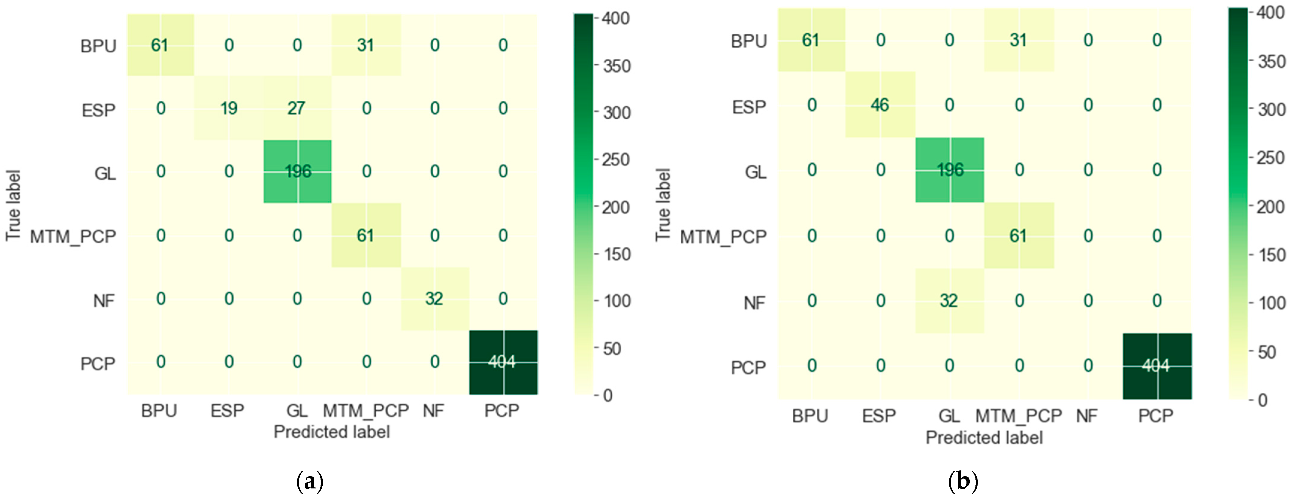
Figure 6 is the classification report (known as the confusion matrix), illustrating the predicted and actual ALs used in the field. We can see that both algorithms effectively predicted BPU, PCP, and ESP. The prediction error of 7.5% resulted in thermal recovery pumps, namely BPU and MTM_PCP, while the 7% error is in GL and NF classification. The wrong prediction of thermal AL is because MTM_PCP has the lowest weight in the dataset; nevertheless, both algorithms predicted it for CSS. The BPU was used in both SF and CSS, while MTM_PCP was only used in CSS wells in the field; thus, the model selected MTM_PCP as more appropriate than the BPU considering input parameters. The RF classifier predicted GL instead of the actual NF label due to the similarity of gas and GOR features. Additionally, NF has approximately the same amount of cumulative GL oil before reservoir energy is depleted and replaced by another lifting method. The DT classifier predicted GL for the actual ESP actual because some ESP wells produce a small amount of gas, which the algorithm principally uses to classify the AL.
The ML application in AL selection seems to be a premature process, as one recent study conducted by [
18] shows.
Table 3 compares this study with [
18] selection results. The highest model training accuracy obtained by [
18] was 94%; no testing scores were mentioned. Our model’s testing accuracy using a separate dataset that it has not been trained on is 93%, indicating satisfactory performance in predicting the optimum lifting methods. Our study proves that the selection could be accomplished using a specific dataset and obtaining the highest accuracy. Another recent interesting study was presented by [
30] to select the optimum AL using fuzzy logic and mathematical models. However, their model is conditioned on an enclosed data inventory of five lifting methods and might not be applicable if different input parameters or other ALs are used instead. Our model is independent of specific datasets; any other data and AL can be modeled. In addition, ref. [
30] tests their model on one well while we test our model on eight wells to substantiate the results.
This study demonstrates that the AL selection could be performed using only production data. The widely used selection techniques in literature, such as selection tables [
5,
31,
32], expert systems [
10], decision trees [
33], and decision-making and ranking models [
34], did not select the optimum AL. Nevertheless, they provide advantages, disadvantages, rankings, and guidelines to eliminate inappropriate AL and recommend other lifting methods. On the other hand, our model directly predicted the optimal AL by learning from the available data. These research findings strengthen [
8] the presumption of invalidation of the conventional selection techniques.
4.2. AL Size Selection Results
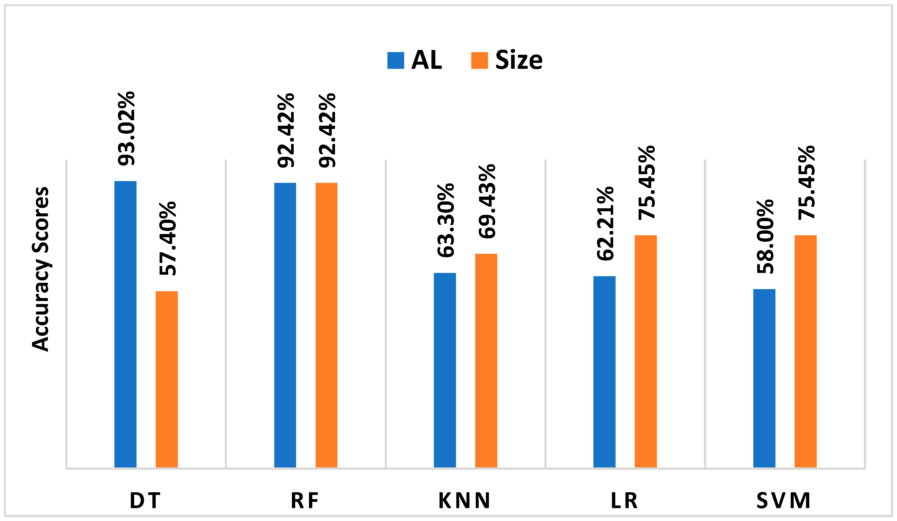
RF was selected for modeling in the AL size selection because of its best performance among the other algorithms. Additionally, it predicted that the AL would have better production performance compared to the DT. The model conducted three runs using 13, 8, and 6 size classes. Unlike AL selection’s high accuracy, the accuracies obtained by the RF classifier on the 13 and 8 classes were 69.68% and 75.74%, respectively. It is evident that many classes of AL size resulted in poor model performance. The rationale is that the distribution of AL sizes over an oil well’s life varies as it continuously changes after years of production. In other words, the continuous replacement of AL sizes led to some sizes appearing in the training dataset (during a specific production period) while disappearing in the test dataset (during another production period). Thus, the model could not find the optimum size to select, although the same AL exists. Operationally, and after years of production, the AL size is replaced due to low productivity, failure, or IOR/EOR implementations. Therefore, it is unlikely to use the same AL type and size for the whole oil well production life because of the change in well and reservoir properties that affects well deliverability over time. RF obtained the highest model accuracy of 92.42% (
Table 4) using the 6 AL size classes (Large, Medium, and Small for PCP, BPU, and MTM_PCP, WSB for ESP, NUE-Mandrel for GL, and X-tree_5000psi used for naturally flowing wells). The other algorithms scored (57–75%) as shown in
Figure 7.
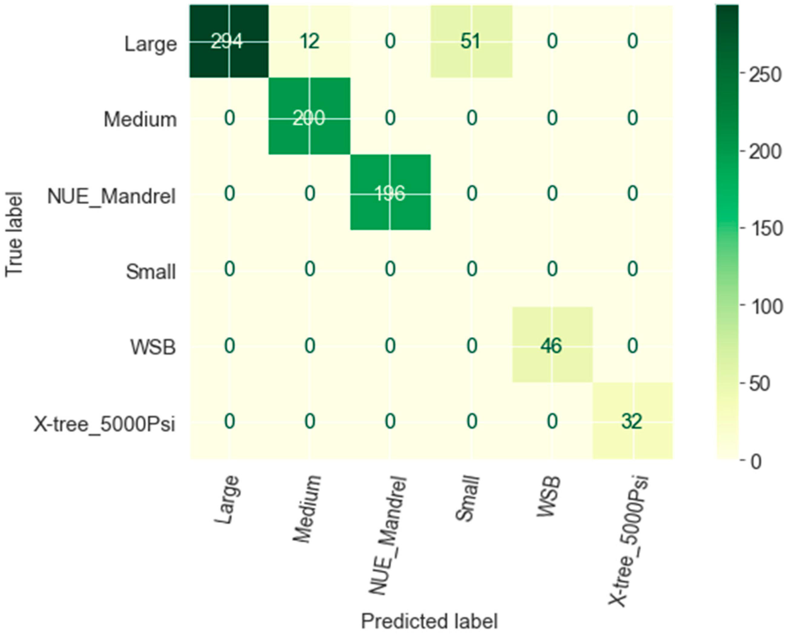
The 7.5% RF prediction error resulted from the two wrongly predicted sizes, Small and Medium, in which Large was the actual size, as illustrated in
Figure 8. The reason is that after years of production, some parameters have similar values, such as flow rates, pressures, production years, and WC%, which are recorded in different sizes.
4.3. Production Performance of Predicted and Actual AL
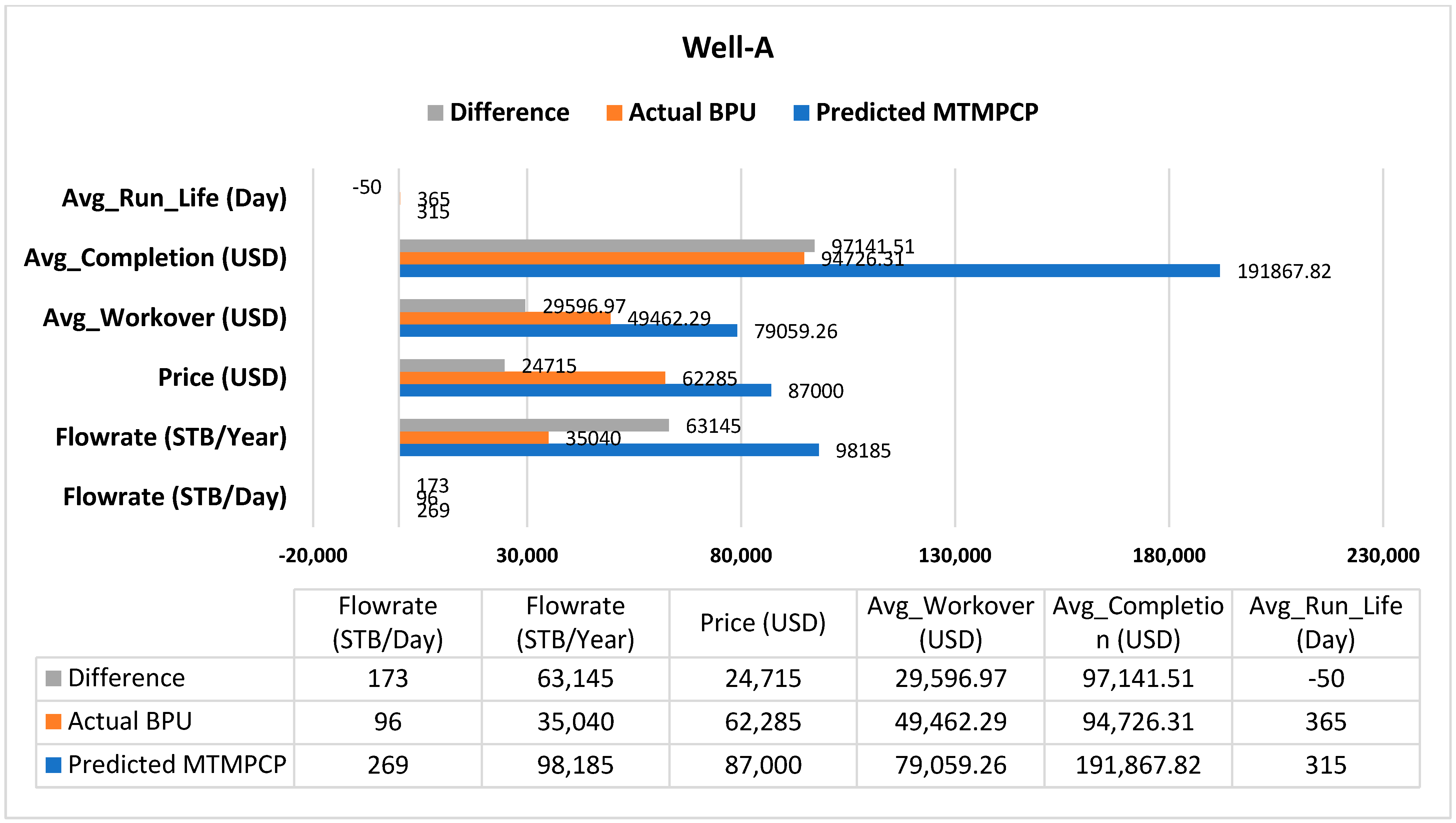
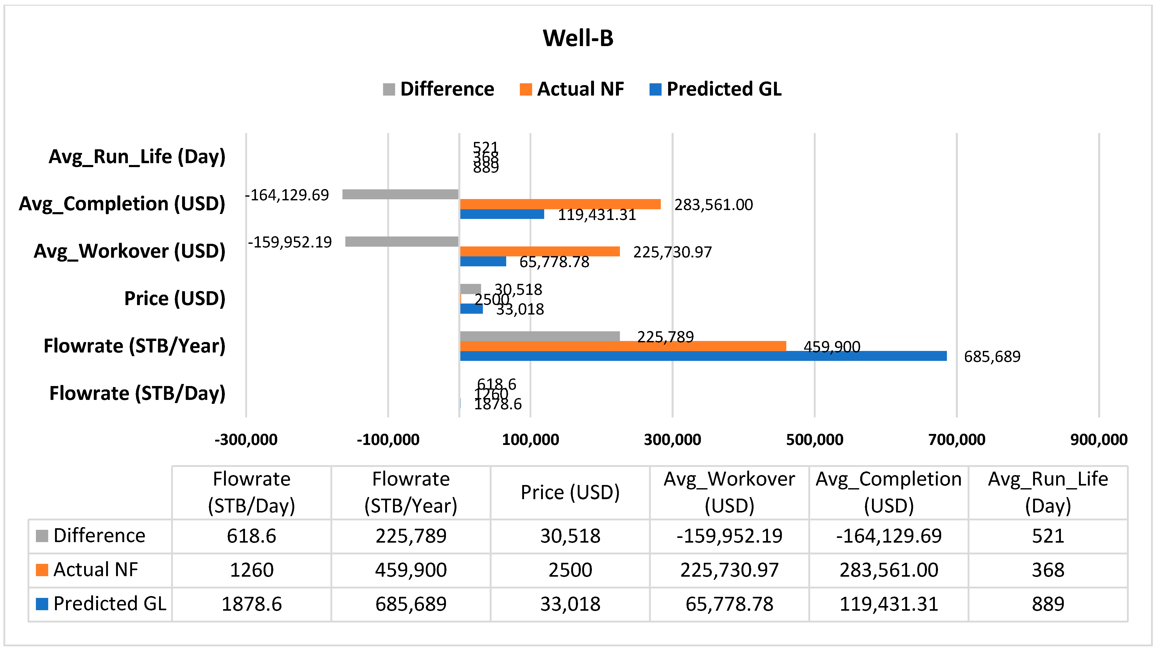
We conducted a simulation using the PIPESIM simulator to model the performance of the predicted AL, well-A, and well-B. Well-A undergoes CSS and is produced by SRP using a thermal sand control pump (275TH7.2S-1.2 Grade-III, Large). Our ML predicted MTM_PCP instead of the current BPU. We simulated well-A production using a MET-80V1000 Medium-size thermal pump. Well-B is naturally flowing using X-tree_5000psi. The well was simulated according to the predicted AL using 3 GL valves. The results showed that the predicted AL from the ML model has better performance than the current installed AL. Well-A can produce 269 STB/D using MTM_PCP, more than the current 97 STB/D by BPU. Well-B can produce 1878 STB/D using GL, compared to its current natural flow production of 1260 STB/D.
Figure 9 and
Figure 10 are the sensitivity analyses of the actual and predicted lifting methods. The figures compare each lifting method’s flow rates, average costs, and run life. The cost of the predicted AL could be higher than the current lifting methods; however, the high production revenues (above 3 million USD from well-A and 11 million USD from well-B) would undoubtedly cover the operating expenses. These case study results are promising for further application in AL selection for prospective wells.
4.4. Critical Production Selection Features
The model also highlighted the critical factors affecting AL and size selection in the field.
Figure 11 illustrates the essential features that the RF used foremost and that affect the AL classification. Gas and produced fluid substantially determine the classification, followed by the wellhead pressure. In other words, the algorithm depends primarily on gas, produced fluid, and wellhead pressure to classify the lifting methods and considers them crucial factors in AL selection. It is worth mentioning that although there was a poor correlation between input parameters, the model obtained classification results above 90%. According to the results, these factors should be extensively studied in any current or prospective oil wells since they determine the production performance. If we take the gas feature of the old selection technique as described in the literature and in the field, we find that it is the worst obstacle to most lifting methods except GL and NF. Our model correctly identified the significance of the gas feature and demonstrated how it could influence AL selection and production performance. The other highlighted critical factors are the produced fluid, GOR, produced water, thermal recovery, and the years of production. The [
30] model lacked any IOR or EOR data that affects AL performance, while [
34] considered it, and our model found it a critical feature in AL classification. [
34] used the production rate as the most highly weighted parameter in their model, supporting the importance of the flow rate feature in our model. Flow rate is a crucial factor in all selection methods in the literature; however, the literature uses only the flow rate limitations of each AL [
5,
31,
32,
33]. These limitations are proposed operating ranges that vary in the literature. Our model studied the daily and cumulative fluid produced during the entire run-life of the AL and provided the optimum lifting method that can last longer with higher production performance, as in the production performance simulation results.
5. Conclusions
AL is a milestone in the oil and gas industry, and this paper introduced a new AL selection approach that can facilitate the selection and save AL parameter screening time in the Sudanese oil fields. The developed model is universal and can be implemented in any other established field using different data and lifting methods. The following conclusions are the result of this research:
The paper introduced a new AL type and size selection approach using ML from specific field production data. The results show the robustness of ML application in AL selection from only field production data;
The application of ML in AL selection will facilitate the process and reduce the time spent using old techniques that are considered outdated to a certain degree;
The predicted ALs have higher production performances and revenues than the actual ones in the field;
Production data from 24 wells from 2006 to 2021 was used for modeling. Data from 2006 to 2019 were used for model training and validation, while data from 2020 to 2021 were used to test model performance;
Although it is complex to correlate the numeric and categorical input parameters, the algorithms determine the crucial factors that primarily affect the selection. Gas, wellhead pressure, produced fluid, GOR, produced water, and years of production are significant in AL and size selection from production data;
The model obtained high AL selection accuracies of 93.02% and 92.4%, respectively, by DT and RF classifiers;
RF scored the same accuracy of 92.42% in AL size selection, whereas other algorithms did not perform well;
Many AL size classes resulted in low model accuracy (69.68% and 75.74% obtained from 13 and 8 classes, respectively);
The case study’s results are promising for further application in other fields’ AL selection.
Author Contributions
Conceptualization, M.A.A.M.; methodology, M.A.A.M.; software, M.A.A.M.; validation, M.A.A.M.; formal analysis, M.A.A.M.; investigation, M.A.A.M.; resources, M.A.A.M.; data curation, M.A.A.M.; writing—original draft preparation, M.A.A.M.; writing—review and editing, M.A.A.M., M.A. and G.O.; visualization, M.A.A.M.; supervision, M.A. and G.O. All authors have read and agreed to the published version of the manuscript.
Funding
This research received no external funding.
Data Availability Statement
The data are not publicly available due to a confidentiality request by the provider. The notebook and code of this study can be provided by the corresponding author upon reasonable request.
Acknowledgments
The authors would like to thank R. Saleem from the University of Aberdeen, M. El-feel from Schlumberger, M. Mahgoub from Sudan University of Science and Technology/Petro-Energy E&P Co. Ltd., Musaab F. Alrahman, Naji, and K. Al-Mubarak from Petro-Energy E&P Co. Ltd., and all the reviewers who participated in the review for their support in finalizing and publishing this article.
Conflicts of Interest
The authors declare no conflict of interest.
References
- Temizel, C.; Canbaz, C.H.; Betancourt, D.; Ozesen, A.; Acar, C.; Krishna, S.; Saputelli, L. A Comprehensive Review and Optimization of Artificial Lift Methods in Unconventionals. In Proceedings of the SPE Annual Technical Conference and Exhibition, Virtual, 19 October 2020. [Google Scholar]
- Lea, J.F.; Clegg, J.D. Chapter 10. Artificial Lift Selection. In Petroleum Engineering Handbook Volume 4: Production Operations Engineering; Society of Petroleum Engineers: Dallas, TX, USA, 2007. [Google Scholar]
- Beckwith, R. Pumping oil: 155 years of artificial lift. J. Pet. Technol. 2014, 66, 101–107. [Google Scholar] [CrossRef]
- Dave, M.K.; Mustafa, G. Performance evaluations of the different sucker rod artificial lift systems. In Proceedings of the SPE Symposium: Production Enhancement and Cost Optimization, Kuala Lumpur, Malaysia, 7 November 2017. [Google Scholar]
- Clegg, J.D.; Bucaram, S.M.; Hein, N.W. Recommendations and Comparisons for Selecting Artificial-Lift Methods (includes associated papers 28645 and 29092). J. Pet. Technol. 1993, 45, 1128–1167. [Google Scholar] [CrossRef]
- Syed, F.I.; Alshamsi, M.; Dahaghi, A.K.; Neghabhan, S. Artificial lift system optimization using machine learning applications. Petroleum 2020, 8, 219–226. [Google Scholar] [CrossRef]
- Shi, J.; Chen, S.; Zhang, X.; Zhao, R.; Liu, Z.; Liu, M.; Zhang, N.; Sun, D. Artificial lift methods optimising and selecting based on big data analysis technology. In Proceedings of the International Petroleum Technology Conference, Beijing, China, 22 March 2019. [Google Scholar]
- Noonan, S.G. The Progressing Cavity Pump Operating Envelope: You Cannot Expand What You Don’t Understand. In Proceedings of the International Thermal Operations and Heavy Oil Symposium, Calgary, AB, Canada, 20 October 2008. [Google Scholar]
- Naderi, A.; Ghayyem, M.A.; Ashrafi, M. Artificial Lift Selection in the Khesht Field. Pet. Sci. Technol. 2014, 32, 1791–1799. [Google Scholar] [CrossRef]
- Espin, D.A.; Gasbarri, S.; Chacin, J.E. Expert system for selection of optimum Artificial Lift method. In Proceedings of the SPE Latin America/Caribbean Petroleum Engineering Conference, Buenos Aires, Argentina, 27 April 1994. [Google Scholar]
- Alemi, M.; Jalalifar, H.; Kamali, G.; Kalbasi, M. A prediction to the best artificial lift method selection on the basis of TOPSIS model. J. Pet. Gas Eng. 2010, 1, 009–015. [Google Scholar]
- Mohamed, A.E. Comparative study of four supervised machine learning techniques for classification. Int. J. Appl. Sci. Technol. 2017, 7, 2. [Google Scholar]
- Makeen, Y.M.; Shan, X.; Ayinla, H.A.; Adepehin, E.J.; Ayuk, N.E.; Yelwa, N.A.; Yi, J.; Elhassan, O.M.; Fan, D. Sedimentology, petrography, and reservoir quality of the Zarga and Ghazal formations in the Keyi oilfield, Muglad Basin, Sudan. Sci. Rep. 2021, 11, 743. [Google Scholar] [CrossRef] [PubMed]
- CNPC Country Reports, CNPC in Sudan 2009. Available online: https://www.cnpc.com.cn/en/crsinSudan/AnnualReport_list.shtml (accessed on 15 January 2022).
- Liu, B.; Zhou, S.; Zhang, S. The Application of Shallow Horizontal Wells in Sudan. In Proceedings of the International Oil and Gas Conference and Exhibition in China, Beijing, China, 8 June 2010. [Google Scholar]
- Akosa, J. Predictive accuracy: A misleading performance measure for highly imbalanced data. Proc. SAS Glob. Forum 2017, 12, 942. [Google Scholar]
- Krawczyk, B. Learning from imbalanced data: Open challenges and future directions. Prog. Artif. Intell. 2016, 5, 221–232. [Google Scholar] [CrossRef] [Green Version]
- Ounsakul, T.; Sirirattaanachatchawan, T.; Pattarachupong, W.; Yokrat, Y.; Ekkawong, P. Artificial lift selection using machine learning. In Proceedings of the International Petroleum Technology Conference, Beijing, China, 22 March 2019. [Google Scholar]
- Brownlee, J. Data Preparation for Machine Learning: Data Cleaning, Feature Selection, and Data Transforms in Python; Machine Learning Mastery: Vermont, Australia, 2020; p. 111. [Google Scholar]
- Kotsiantis, S.B.; Zaharakis, I.; Pintelas, P. Supervised machine learning: A review of classification techniques. Emerg. Artif. Intell. Appl. Comput. Eng. 2007, 160, 3–24. [Google Scholar]
- Osisanwo, F.Y.; Akinsola, J.E.T.; Awodele, O.; Hinmikaiye, J.O.; Olakanmi, O.; Akinjobi, J. Supervised machine learning algorithms: Classification and comparison. Int. J. Comput. Trends Technol. (IJCTT) 2017, 48, 128–138. [Google Scholar]
- Gianey, H.K.; Choudhary, R. Comprehensive review on supervised machine learning algorithms. In Proceedings of the 2017 International Conference on Machine Learning and Data Science (MLDS), Noida, India, 14–15 December 2017; IEEE: New York, NY, USA, 2017; pp. 37–43. [Google Scholar]
- Jurafsky, D.; Martin, J.H. Speech and Language Processing, (draft) edition; Prentice Hall: Hoboken, NJ, USA, 2021; Chapter 5. [Google Scholar]
- Mathur, A.; Foody, G.M. Multiclass and binary SVM classification: Implications for training and classification users. IEEE Geosci. Remote Sens. Lett. 2008, 5, 241–245. [Google Scholar] [CrossRef]
- Fletcher, T. Support Vector Machines Explained; Tutorial paper; University College London: London, UK, 2009; pp. 1–19. [Google Scholar]
- Taunk, K.; De, S.; Verma, S.; Swetapadma, A. A brief review of nearest neighbor algorithm for learning and classification. In Proceedings of the 2019 International Conference on Intelligent Computing and Control Systems (ICCS), Madurai, India, 15–17 May 2019; IEEE: New York, NY, USA, 2019; pp. 1255–1260. [Google Scholar]
- Tan, P.N.; Steinbach, M.; Kumar, V. Classification: Basic concepts, decision trees, and model evaluation. Introd. Data Min. 2006, 1, 145–205. [Google Scholar]
- Breiman, L. Bagging predictors. Mach. Learn. 1996, 24, 123–140. [Google Scholar] [CrossRef] [Green Version]
- Hastie, T.; Tibshirani, R.; Friedman, J. Random forests. In The Elements of Statistical Learning; Springer: New York, NY, USA, 2009; pp. 587–604. [Google Scholar]
- Crnogorac, M.; Tanasijević, M.; Danilović, D.; Karović Maričić, V.; Leković, B. Selection of Artificial Lift Methods: A Brief Review and New Model Based on Fuzzy Logic. Energies 2020, 13, 1758. [Google Scholar] [CrossRef] [Green Version]
- Neely, B.; Gipson, F.; Clegg, J.; Capps, B.; Wilson, P. Selection of artificial lift method. In Proceedings of the SPE Annual Technical Conference and Exhibition, San Antonio, TX, USA, 4 October 1981. [Google Scholar]
- Brown, K.E. Overview of artificial lift systems. J. Pet. Technol. 1982, 34, 2384–2396. [Google Scholar] [CrossRef]
- Heinze, L.R.; Winkler, H.W.; Lea, J.F. Decision Tree for selection of Artificial Lift method. In Proceedings of the SPE Production Operations Symposium, Oklahoma City, OK, USA, 9–10 April 1995. [Google Scholar]
- Adam, A.M.; Mohamed Ali, A.A.; Elsadig, A.A.; Ahmed, A.A. An Intelligent Selection Model for Optimum Artificial Lift Method Using Multiple Criteria Decision-Making Approach. In Proceedings of the Offshore Technology Conference Asia, Kuala Lumpur, Malaysia, 18 March 2022; OnePetro: Kuala Lumpur, Malaysia, 2022. [Google Scholar]
| Disclaimer/Publisher’s Note: The statements, opinions and data contained in all publications are solely those of the individual author(s) and contributor(s) and not of MDPI and/or the editor(s). MDPI and/or the editor(s) disclaim responsibility for any injury to people or property resulting from any ideas, methods, instructions or products referred to in the content. |
© 2023 by the authors. Licensee MDPI, Basel, Switzerland. This article is an open access article distributed under the terms and conditions of the Creative Commons Attribution (CC BY) license (https://creativecommons.org/licenses/by/4.0/).


