Article

Role of Non-Renewable Energy Efficiency and Renewable Energy in Driving Environmental Sustainability in India: Evidence from the Load Capacity Factor Hypothesis

1
CREDS-Centre for Research on Digitalization and Sustainability, Inland Norway University of Applied Sciences, 2418 Elverum, Norway
2
Faculty of Economics, Administrative and Social Sciences, Nisantasi University, Istanbul 34398, Turkey
3
Department of Business Administration, Faculty of Economics and Administrative Sciences, Tokat Gaziosmanpasa University, Tokat 60250, Turkey
4
Economics and Finance Application and Research Center, İstanbul Ticaret University, Istanbul 34445, Turkey
*
Author to whom correspondence should be addressed.
Energies 2023, 16(6), 2847; https://doi.org/10.3390/en16062847
Submission received: 14 February 2023 / Revised: 6 March 2023 / Accepted: 17 March 2023 / Published: 19 March 2023

Abstract

:
Policymakers and environmental scientists have proposed numerous measures toward achieving a sustainable environment. Some of these measures include the efficient use of energy and a clean energy transition. This study empirically investigates the role of non-renewable energy efficiency and renewable energy utilization in driving environmental sustainability in India over the period from 1965 to 2018. Using the approach of the Dynamic Autoregressive Distributed Lag (DyARDL) simulations, the empirical evidence shows that non-renewable energy efficiency and renewable energy utilization promote environmental sustainability through an increase in the load capacity factor. The effects of financial development and trade impede environmental sustainability through a decrease in the load capacity factor. The results further show that the relationship between income and load capacity factor is characterized by an inverted U-shape. This suggests that the load capability curve (LCC) hypothesis is not valid for India. Given the overall findings of this study, it is suggested that policymakers should promote energy efficiency and renewable energy technologies as the ultimate policy measure to mitigate the accumulation of CO2 emissions and other significant climatic changes in India.

1. Introduction

As reported by the Global Footprint Network (GFN), India’s ecological footprint exceeds its biocapacity by 171 percent, thus suggesting a significant imbalance in the interplay of its population needs and the nation’s earth supplies, i.e., the load capacity factor (LCF) [1]. Although several reasons could be linked with the increase in the ecological footprint of a country, trade liberalization that allows the importation of biocapacity aspects, the liquidation of national ecological assets, and atmospheric pollution arising from carbon dioxide (CO2) emissions are some of the reasons adduced to the ecological footprint deficit by the GFN. In the case of India, though the country has mostly suffered from trade imbalance over the years [2], the role of trade in economic development cannot be over-emphasized, especially in merchandise and services. Although the contribution of trade to the country’s gross domestic product (GDP) decreased from about 56 percent in the 2011–2012 period to about 45 percent in 2021 [3], the country has continued to experience growth in its exports and imports. This alludes to the potential reason attributed to the ecological deficit, i.e., importation of biocapacity aspects is India’s trade imbalance. For instance, even though export values of all traded commodities increased from over 291 billion United States Dollars (USD) in the period 2020/2021 to over 422 billion USD in 2021/2022 (approximately 44 percent increase), the value of the imported goods and services across the same period increased by 55 percent (i.e., imported products were worth ~394 percent during 2020/2021 and ~613 percent in 2021/2022) (Ministry of Commerce and Industry, 2022). Beyond the above-mentioned factors, the energy consumption mix [4,5] and financial development, among others [6,7], are found to be contributing to India’s environmental quality.
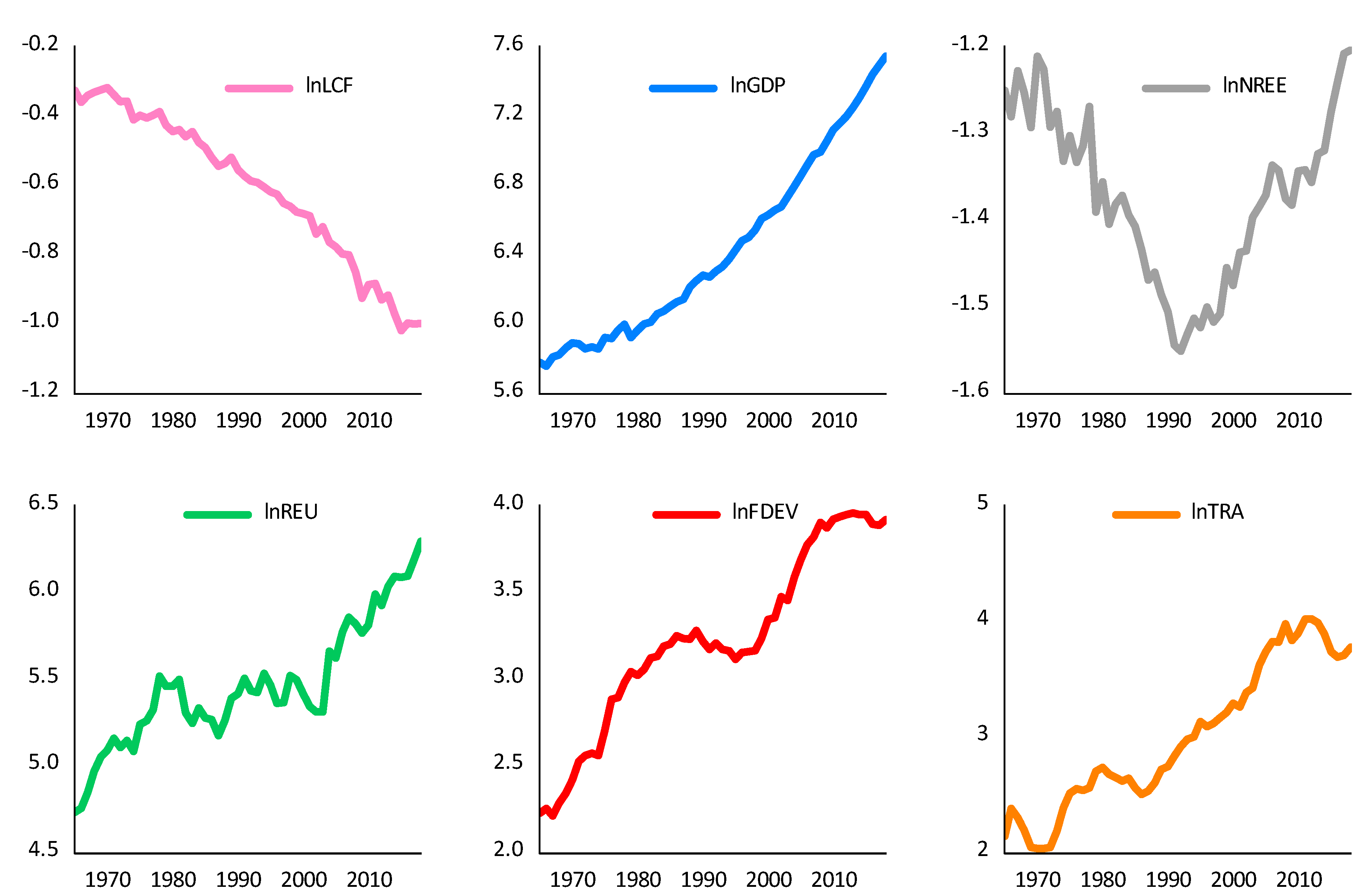
Given the above-mentioned potential drivers of the declining LCF in India (evidently illustrated in Figure 1), how variables such as trade, financial system development, energy efficiency, renewables, and a host of other variables affect LCF still remain unclear. Therefore, the current study is geared towards exposing more fundamental factors driving the ecological footprint–biocapacity nexus. Specifically, the objective of this study is to determine whether the efficient utilization of conventional energy and a clean energy transition influence the LCF capacity factor in India. Additionally, the roles of financial development and trade openness alongside dynamic growth are also explored. As mentioned above, trade makes a significant contribution to the GDP of India, and this justifies the need to examine its influence on the country’s LCF. Moreover, the role of the (in)efficient utilization of conventional energy, i.e., non-clean energy efficiency, has rarely been explored in the literature, which, thus, also justifies the direction of this study. Additionally, the LCC hypothesis was tested in this study by deploying an estimation approach known as Dynamic Autoregressive Distributed Lag (DyARDL). Considering the above-mentioned benefits of the study’s primary objective, this study is therefore poised to yield a significant contribution to the existing literature in several ways: First, the study diverts from the conventional way of determining the drivers of environmental sustainability by applying the LCF as a measure of environmental quality. This is perhaps expected to provide better findings than other measures such as CO2 emissions, greenhouse gas emissions, ecological footprints, etc. Second, this study tests the validity of the LCC hypothesis for India by incorporating variables such as trade and financial development. Third, Dynamic Autoregressive Distributed Lag (DyARDL) simulations were applied. This approach makes it possible to assess the short-run and long-run impacts of both positive and negative changes in explanatory variables on the LCF.
The remaining sections of this study are arranged as follows. Section 2 reviews the related studies. Section 3 describes the data and empirical model for the study. Section 4 presents the results and discussion of the findings. The final section, i.e., Section 5, concludes and make policy suggestions based on the findings of the study.

2. Review of Related Literature

The determination of the drivers of the LCF is rooted in the fundamental study of the atmospheric impacts [8,9]. In the current context, the LCC hypothesis models after the environmental Kuznets curve (EKC) hypothesis [10]. Therefore, the follow-up subsection is dedicated to the review of related studies within the framework of the mentioned EKC.

2.1. LCF and Energy Mix

In the study of [11], the validity of the LCC hypothesis for France during the period 1977–2017 was examined from the perspective of renewable and nuclear energy. Using the Fourier transformed approaches of cointegration and causality, the results revealed a lack of an EKC hypothesis when carbon emission was employed as an environmental variable, but they validated the EKC with the LCF. Importantly, the results further showed that nuclear energy mitigated carbon emissions and increased the LCF in the long-run, thus justifying nuclear energy’s effectiveness in improving environmental quality against renewable energy that acts in the opposite direction. Ref. [12] used three different indicators of environmental quality, namely, CO2 emissions, ecological footprints, and LCF, to examine the influence of nuclear energy use on environmental quality in South Korea. By employing the ARDL estimation approach, the study found that the load capacity curve and environmental Kuznets curve were validated. It further revealed that nuclear energy displayed a positive impact on environmental quality by dampening the level of carbon emissions, while renewable energy evidently displayed no impact on the state of the environment.
Similarly, [13] explored the case of Turkey during the period 1965–2017 by using the dynamic approach of the Autoregressive Distributed Lag (ARDL). The indicators examined, including aggregated energy consumption, tourism arrivals, and GDP, were all responsible for a decline in local capacity factor, which is an indication that the increase in the indicators is detrimental to environmental quality in the country. More recently, [14] looked at how economic growth, financial development, and tourism affected three measurements of environment indicators and, thus, tested the validity of the EKC and LCC hypotheses for the top ten tourism destinations in the world. Using second-generation panel data analytical techniques, the authors provided empirical evidence that both the EKC and LCC hypotheses were not valid in this case, although tourism arrivals improved environmental quality, while the development of the financial sector dampened the LCF.

2.2. Trade, Financial Development, and LCF

Like other environmental indicators, the LCF is found to be influenced by financial development [15,16]. Specifically, [15] employed the approaches of time frequency domain causality and dual adjustment for the case of India and found that financial globalization, clean energy transition, and resource endowments increased the LCF, i.e., improved environmental quality in the long-run, as the impact of economic growth was detrimental to LCF, i.e., the environmental quality. Meanwhile, the short-term effect showed that only renewable energy use was detrimental to the LCF in the short-run by causing a decline in the country’s load capacity factor. The case of Brazil was similarly considered in the recent study of [16] by using the ARDL approach for the data period 1970–2017. While the study affirmed that financial globalization increased the LCF i.e., improved environmental quality in Brazil as revealed by the result, a renewable and non-renewable energy mix alongside economic growth were responsible for the decline in the LCF.
As recently investigated, trade was also found to influence the LCF in Mexico while considering the dataset that covered the period 1970–2017 by [17]. The implemented dual adjustment approach affirmed cointegration among the LCF, renewable energy utilization, non-renewable energy utilization, economic growth, and trade openness over the examined period. Furthermore, trade openness was found to increase the LCF in the long-term, thus affirming the environmental desirability of trade liberalization in Brazil as against the negative impact of other indicators on the LCF. Of course, the study of [18] showed a contrary perspective on the effect of trade openness on the LCF. Specifically, [18] implemented several quantile approaches, including quantile regression and quantile-on-quantile regression, for the case of Turkey over the time from 1965–2018 and revealed that the LCF was negatively affected by trade openness. Moreover, the LCF was also negatively impacted by the increase in financial development and primary energy utilization across most of the quantiles.
Importantly, as is evident from the review of the above studies, a notable gap in the literature exists regarding the lack of a body of knowledge that suggests the drivers of the LCF from a comparative analysis of non-renewable energy efficiency and renewable energy use. Therefore, to further cover the existing deficiency in the body of knowledge, the LCF effect due to non-renewable energy efficiency and renewable energy use, alongside the roles of trade openness and financial development, were examined.

3. Data Description and Modeling Techniques

3.1. Description of Data

The paper employs the multivariate annual time-series data spanning the period from 1965 to 2018 for empirical investigation. This time was dictated by data availability. The dependent variable of the study is the LCF, and we chose this variable as a measure of environmental deterioration by following the studies of [11,13,15]. The LCF represents a particular ecological threshold by comparing biocapacity and ecological footprint, and a rise in the LCF indicates an increase in environmental quality, while its decrease implies a surge in environmental degradation. The fact that the LCF considers both the supply and demand sides of environmental issues has made it a more comprehensive indicator than traditional environmental damaging indicators such as CO2 emissions and ecological footprint. Because of these important properties, we used the LCF as a proxy for environmental degradation in this study instead of the traditional CO2 emissions or ecological footprint.
Furthermore, we used economic growth, non-renewable energy efficiency, renewable energy usage, financial development, and trade openness as independent variables. We measured economic growth as the gross domestic product (GDP) per capita, which follows [19]. As freely available in online database, the GDP series is retrieved from the World Development Indicators of the World Bank (WDI) as measured in constant 2015 USD per capita. Since one of the most important reasons for energy usage is to generate income, unlike the existing literature, we used non-renewable energy efficiency, which measures the non-renewable energy that needs to be consumed to generate an income of 1 USD, instead of classical non-renewable energy usage. We calculated non-renewable energy efficiency as GDP Non-renewable   energy   usage , where non-renewable energy usage series were taken from the Our World in Data (OWD) as kWh per capita. We also downloaded the kWh per capita renewable energy usage series from OWD (See the link Our World in Data: https://ourworldindata.org/ (accessed on 24 December 2022). By following [20,21,22], we utilized the domestic credit to private sector (% of GDP) series gathered from the WDI as a proxy for financial development. Finally, we measured trade openness as the sum of exports and imports (i.e., trade) based on the research of [23,24,25]. The trade series were extracted as a percentage of GDP from the WDI. Details regardings the variables we have explored are also provided in Table 1.
All study variables were transformed into natural logarithms to minimize size variability between the variables and heteroscedasticity issues. Figure 1 displays the time-series plots of the annual logarithmic values of all variables used for this study. From the figure, it is seen that the LCF of India had a decreasing trend over the study period, i.e., 1965 to 2018, while gross domestic product (GDP), renewable energy usage, financial development, and trade openness had an increasing trend over the study period, i.e., 1965 to 2018. Nevertheless, the non-renewable energy efficiency of India decreased until the late 1990s, after which, it started increasing. This could be due to policy changes introduced by the Indian government over time. Furthermore, based on all the series employed in this study, there was no high level of fluctuations caused by structural breaks.
The descriptive statistics of the examined variables provided in Table 2 include the mean, median, maximum, minimum, standard deviation, skewness, kurtosis, and Jarque–Bera. The mean values show that, between 1965 and 2018 in India, the annual average of logarithmic values of the LCF was −0.609, the gross domestic product was 6.431, the non-renewable energy efficiency was −1.373, the renewable energy usage was 5.460, the financial development was 3.214, and the trade openness was 2.998. According to the standard deviation values, trade openness had the highest volatility, followed by GDP and financial development, while non-renewable energy efficiency had, by far, the lowest volatility. Based on the skewness and kurtosis values, we concluded that the distribution of the GDP, REU, and TRA was positively skewed, whereas that of the LCF, NREE, and FDEV was skewed leftward. Also, the values of the kurtosis suggest that all variables had a platykurtic distribution. Furthermore, the results of the [26] test of normality disclose that our variables were normally distributed during the sample period.

3.2. Model & Methodology

This study empirically explores the dynamic impact of non-renewable energy efficiency, renewable energy usage, financial development, and trade openness on the LFC. We checked the hypothesis of the LCC for the case of India using the function and econometric model shown below:
l n L C F = f l n G D P ,   l n G D P 2 ,   l n N R E E ,   l n R E U ,   l n F D E V ,   l n T R A
l n L C F t = 0 + 1 l n G D P t + 2 l n G D P t 2 + 3 l n N R E E t + 4 l n R E U t + 5 l n F D E V t + 6 l n T R A t + ε t
where Equation (1) is the exact functional specification of the model, while Equation (2) provides the econometric model for the study. In the equation specified above, t symbolizes time, the constant term is denoted by 0 , the natural logarithm is represented by l n , the LCF is denoted by L C F , the gross domestic product is denoted by G D P , the square of GDP is symbolized by G D P 2 , the non-renewable energy efficiency is represented by N R E E , the renewable energy usage is represented by R E U , the financial development is represented by F D E V , and trade openness is represented by T R A . Moreover,   1 , 2 , 3 , 4 , 5 , and 6 represent coefficients of the predictor variables, and ε t stands for the error term.
This study utilized the novel DyARDLS model that was first established through the empirical work of [28] for empirical analysis. The DyARDLS technique is a modified version of the conventional ARDL approach proposed by [29]. In the case of complicated requirements (i.e., multiple lags, 1st differences, and lagged 1st differences, etc.), it may be difficult to realize short-run and long-run impacts of the independent variables on the dependent variable with the traditional ARDL estimation technique. On the other hand, the DyARDLS technique simulates, forecasts, and provides plots automatically for the effects of the possible counterfactual changes, which occur at a specific time, of an independent variable on the predicted variable while taking the remaining independent variables as constant by using dynamic stochastic simulation techniques. Therefore, the DyARDLS model allows us to easily understand the short-run and long-run impacts of both positive and negative changes in independent variables on the dependent variable [28]. Because of these distinctive features, the DyARDLS approach was adopted for this study.
The model of the DyARDLS in error correction format can be presented as follows:
Δ l n L C F t = 0 + 0 l n L C F t 1 + σ 1 Δ l n G D P t + ω 1 l n G D P t 1 + σ 2 Δ l n G D P t 2 + ω 2 l n G D P t 1 2 + σ 3 Δ l n N R E E t + ω 3 l n N R E E t 1 + σ 4 Δ l n R E U t + ω 4 l n R E U t 1 + σ 5 Δ l n F D E V t + ω 5 l n F D E V t 1 + σ 6 Δ l n T R A t + ω 6 l n T R A t 1 + ε t
where Δ specifies the first difference operator, 0 represents the constant term of the estimation, the error correction term coefficient is symbolized by 0 , σ i ’s (for i = 1, 2, 3, 4, 5, 6) are the short-term coefficients, ω i ’s (for i = 1, 2, 3, 4, 5, 6) are the long-term coefficients for each explanatory variable, and ε t stands for the model’s error term.

4. Empirical Results

For the DyARDLS model results to be valid, the order of integration of any variable under consideration must not be second difference, i.e., I(2). In other words, the variables’ order of integration can be at level, i.e., I(0), or first difference, i.e., I(1) [30,31,32,33]. Also, the co-integration relationship must be between the variables under consideration. For these reasons, three widely used unit root tests, namely, Augmented Dickey–Fuller [34], Phillips–Perron [35], and Zivot–Andrews [36] (ZA) were first used to make sure the order of integration of any of the variables was not I(2) (corroborated in the literature [37,38,39,40,41]) also apply these unit roots). The unit root test results are reported in Table 3. The results of these unit root tests disclose that the null hypothesis of non-stationary could be rejected at the first difference for all variables, which implied that the order of integration for all the variables employed in this study was I(1). The implication of these results is that no variable exceeded the order of integration allowed to proceed with the estimation of the DyARDLS.
Table 4 reports the outcomes of the information criterion for lag selection. From the table, two out of five different criteria, selected the same value; that is, the lag order of three was selected by the LR and FPE, whereas one was selected by the SC and HQ. As was mentioned by [42], the AIC, SC, and HQ are among the most widely used criteria, and therefore we chose the lag order of one selected by the SC and HQ in this study.
Since the order of integration of any study variable was not I(2), and the optimal lag length was one, we then applied the [29] Pesaran–Shin–Smith (PSS) cointegration test of to assess whether there was a co-integration relationship between the variables under consideration or not. In the study, we used the critical values of [43] for the lower and upper bounds of each significance level, since these values give more robust and reliable outputs, especially for the small sample size as in this study. According to the results of the PSS cointegration test reported in Table 5, the null hypothesis of no co-integration relationship could not be true, since the F-statistic value (4.77) was greater than the upper bound value (4.00) at the 5% significance level, and the absolute value of the t-statistic (5.27) was greater than the absolute value of the upper bound (4.99) at the 1% significance level. Overall, these results prove that a valid co-integration relationship existed between the study variables.
After the requirements for estimating our model were attained, i.e., having variables that are integrated of not more than I(1) and also cointegrated, we then applied the DyARDLS method to obtain the short- and long-run parameters of the estimates. The statistically significant short- and long-run coefficients estimated by the DyARDLS are plotted in Figure 2. At a glance, it is evident that GDP had the highest short- and long-run coefficients. Since these coefficients were positive, we concluded that there is a positive association between GDP and the LFC in India. Statistically, a 1% increase in GDP surged the LFC in India by 4.87% in the short run and 1.29% in the long run, thus implying that a positive contribution of income to environmental damage decreased over time. On the other hand, the short-term and long-term parameters of the GDPSQ were negative, which means that there was a negative linkage between the GDPSQ and the LFC. A 1% rise in the GDPSQ decreased the LFC by 0.41% and 0.12% in the short term and long term in India. This result discloses that increasing GDP not only reduces the positive influence of income on environmental damage but also, after a certain point, begins to harm the environment in India. Also, both the GDP and GDPSQ parameters clearly show that there was an inverted U-shaped relationship between income and the LFC. This reveals that the LCC hypothesis is not valid for India; however, the inverted U-shaped interaction between income and LFC signifies that the EKC assumption is perhaps valid for India.
Furthermore, Figure 2 demonstrates that the short- and long-term coefficients of both non-renewable energy efficiency and renewable energy use were positive, thus indicating that the LFC (i.e., environmental quality) was positively affected by non-renewable energy efficiency, or clean energy use, in India. Specifically, a 1% increase in non-renewable energy efficiency increased the LFC by 0.28% in the short run and by 0.34% in the long run, while a 1% increase in renewable energy use resulted in an approximately 0.09% increase in the LFC in both the short and long term. These results reveal that, although non-renewable energy efficiency and renewable energy use are favorable factors for environmental sustainability, non-renewable energy efficiency had a much greater impact on environmental quality than renewable energy use in India. Lastly, it is seen that financial development and trade had very close negative coefficients that were statistically significant in the long run. This means that financial development and trade exerted almost the same negative effect on the LFC in India in the long run. Specifically, a 1% upsurge in financial development and trade decreased the LFC by 0.07% and 0.06% in the long run, respectively. These results divulge that both financial development and trade degrade the environment in India, albeit to a small extent.
We performed a set of diagnostic tests to assess whether the findings of this study from the DyARDLS method were robust and reliable. The outputs of the diagnostic tests are reported in Table 6. The results in Table 6 show that the model used in the analysis had no serial correlation, heteroscedasticity, ARCH effect, misspecification, and non-normality issues. The results of diagnostic tests also support that the findings obtained from the DyARDLS method were reliable and robust.
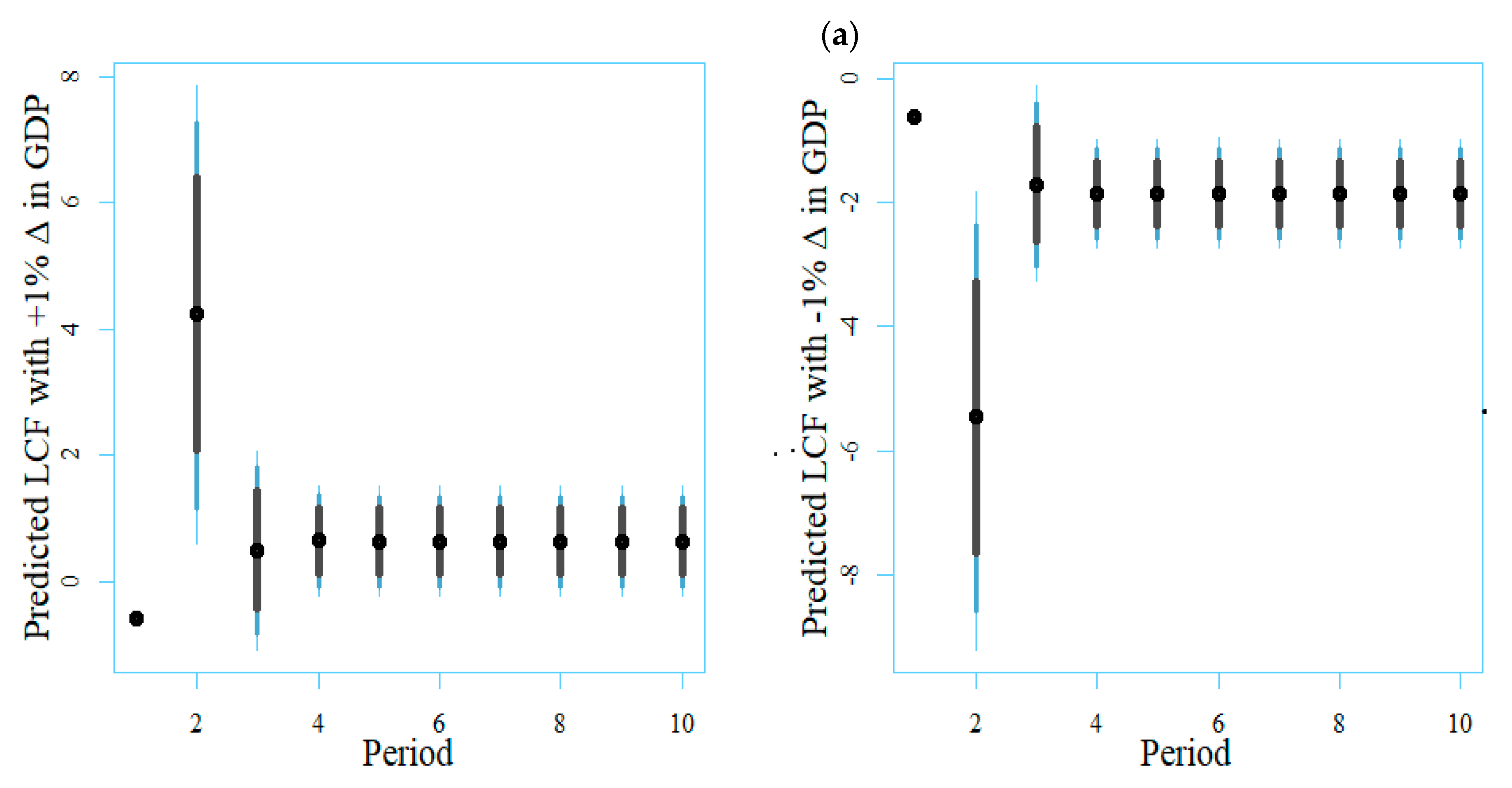
As previously stated, one distinguishing feature of the DyARDLS method is that it automatically generates impulse–response plots that project how a counterfactual positive and negative change in an independent variable affects the future path of the dependent variable while holding the remaining independent variables constant. We examined the impulse–response plots obtained from the DyARDLS method to investigate the dynamic impact of a one percent positive and negative change in our independent variables on the LFC in India. Figure 3a–f show the response of the LFC a 10-year period to ±1% counterfactual change occurring in the second year for GDP, GDP2, non-renewable energy efficiency, renewable energy use, financial development, and trade, respectively.
The impulse–response plots in 
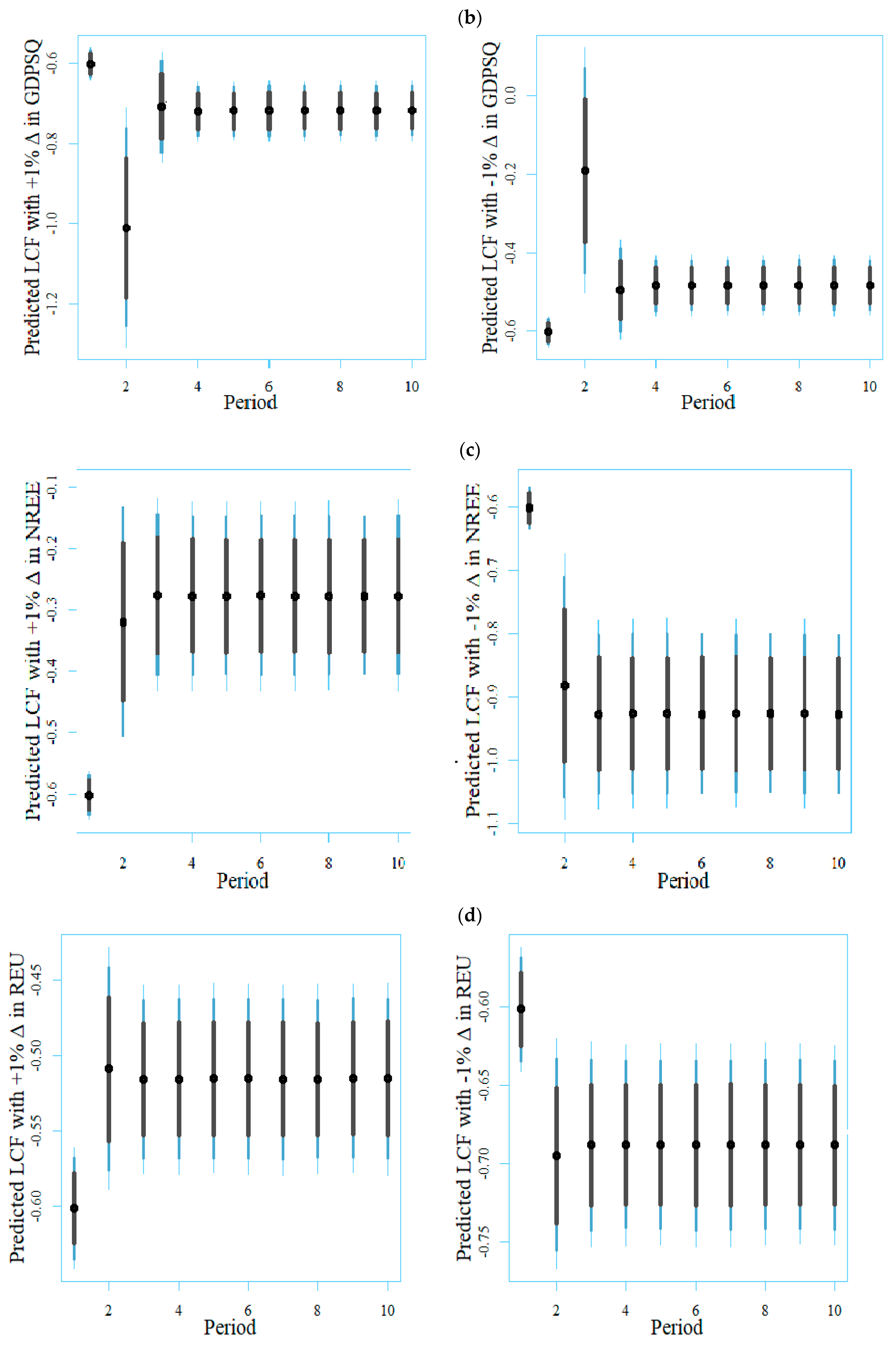
Figure 3a,b show that a 1% positive (negative) change in GDP increased (decreased) the LCF, while a 1% positive (negative) change in GDPSQ had the opposite effect in India. The fact that GDP increased and GDPSQ decreased the LCF reveals that there was an inverted U-shaped linkage between income and LCF, and, therefore, the LCC hypothesis is not valid for India. Also, the impulse–response plots in Figure 3c,d demonstrate that the LCF responded positively (negatively) in India to the impulse of a 1% increase (decrease) in non-renewable energy efficiency and renewable energy use. Notably, the impact of non-renewable energy efficiency on the LCF was greater than renewable energy use. These results suggest that India should increase renewable energy usage, as well as make more efficient use of non-renewable energy.
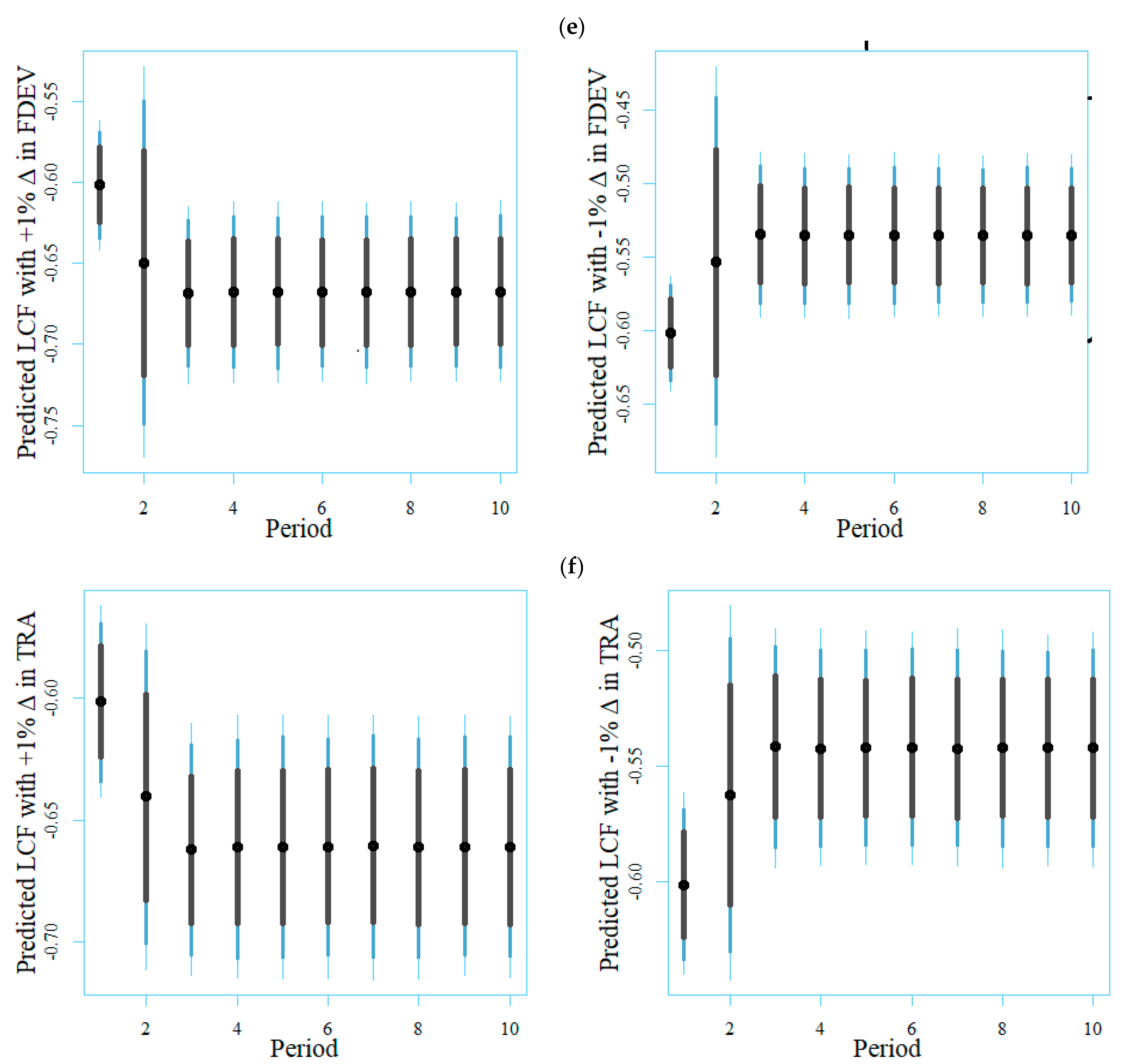
Furthermore, the impulse–response plots in Figure 3e,f illustrate that a 1% positive (negative) change in both financial development and trade declined (rose) the LCF by almost the same amount in India. This means that increasing financial development and trade have had an adverse effect on India’s environmental quality, and, thus, India should ensure that the incomes generated by financial development and trade openness are shifted to more environmentally friendly investments with the necessary incentives by determining the current usage areas.
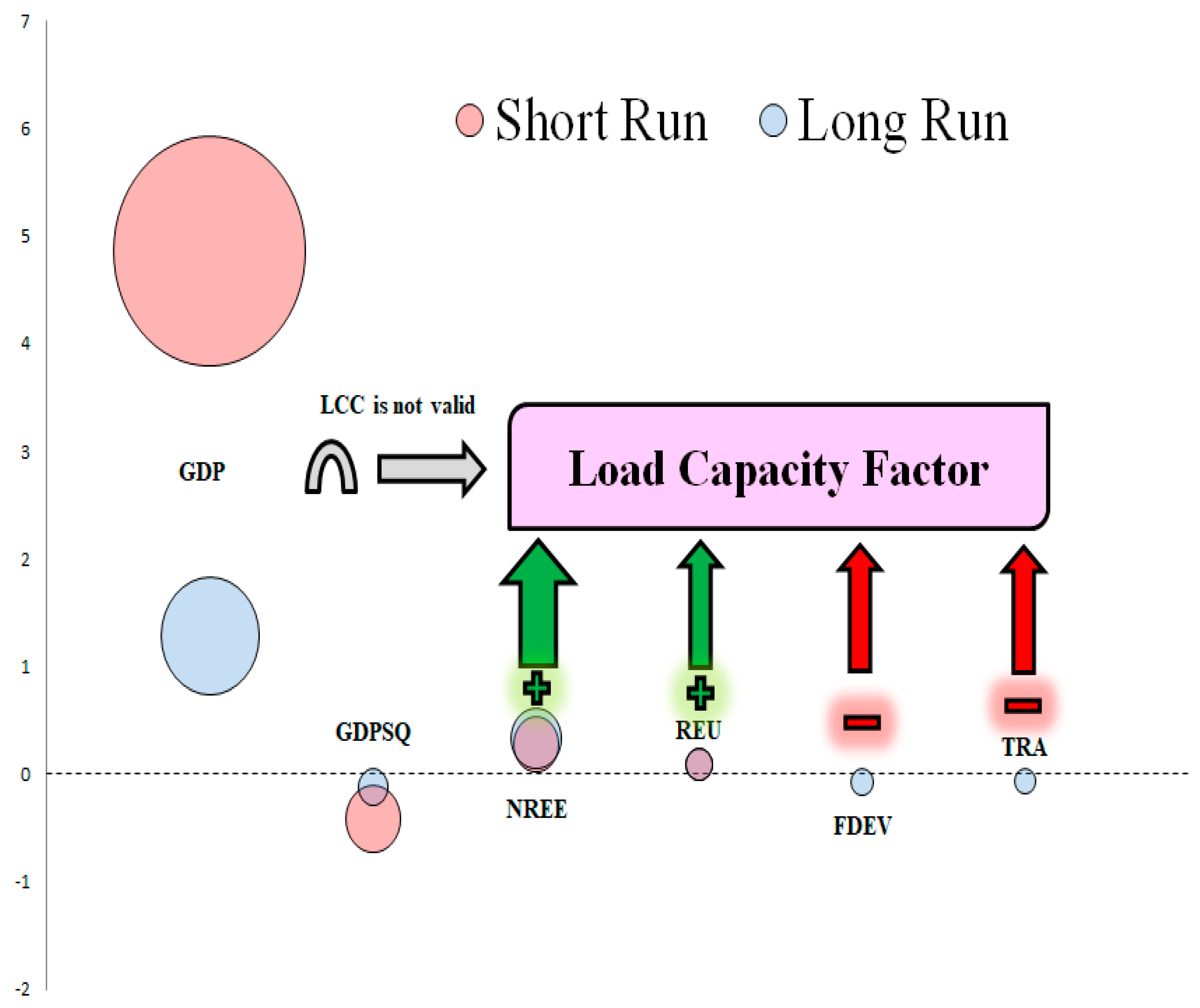
Finally, the study findings are summarized in Figure 4. As can be seen from the figure, the y-axis represents the coefficients expressed in absolute values, which also connotes the size of the bubbles. The −1 and +1 changes in a certain variable have the same bubble size. The x-axis reveals the explanatory variables in the model. The GDP (GDPSQ) had a positive (negative) impact on the LCF both in the short and long run; that is, income had an inverted U-shaped impact on the LCF, and, thus, the LCC hypothesis is not valid in India. The impact of non-renewable energy efficiency and renewable energy use on the LCF was positive in India, both in the short and long run. In addition, the impact of non-renewable energy efficiency on the LCF was greater than renewable energy use. At last, financial development and trade had nearly the same magnitude of long-term negative impact on the LCF in India.

Discussion of Findings

From the results of this study, it is clear than an increase in GDP reduced the LCF, while its square term increased the LCF. This suggests that the LCC hypothesis is not invariably supported by this study. The failure of the result of this study to uphold the LCC hypothesis for India suggests that the EKC hypothesis is obviously valid for India. Therefore, our finding is consistent with [44], who found that the EKC assumption was established in India after controlling for the effect of energy consumption and democracy. Also, our finding is in agreement with the recent findings documented by [11,12] who found that, there was no evidence supporting the LCC assumption for France and South Korea, respectively. Conversely, our finding is not supported by the main conclusion put forward by [14] that significant evidence in support of both the EKC and LCC assumptions was found for the top ten tourism destinations. The implication of the confirmation of the EKC assumptions is that an increase in economic growth is associated with environmental damage until a threshold value is established. On the other hand, the confirmation of the LCC assumption implies that growth is associated with environmental improvement. This is a signal that green growth is associated with the development pattern in these two economies, i.e., France and South Korea.
Furthermore, our results show that both nonrenewable energy efficiency and renewable energy utilization dampened the level of environmental degradation in India by improving the level of the LCF. The plausible explanation for the positively significant effect of nonrenewable energy efficiency established in this study suggests that fossil fuels, when used efficiently, can lead to environmental improvement. This finding is possibly pointing to the fact that technological advancement is a vehicle that promotes energy efficiency. By this revelation, it means that, in addition to the environmental lessening effect of renewable energy, nonrenewable energy efficiency can guarantee a sustainable environment. Therefore, the positive effect of renewable energy is consistent with [15], who found that financial globalization and renewable energy promoted the LFC in India. Similarly, our results are also consistent with [16], who found financial globalization, renewable energy, and non-renewable energy stimulated the LFC, while economic growth dampened it in the case of Brazil. Furthermore, the negative effect of trade and financial development is in agreement with [18], who showed that trade and financial development reduced the LFC.
Furthermore, the negative effects of financial development and trade suggest that, as India is opening up to trade and stimulating financial development policies, the level of the LCF is reducing, which is thereby increasing environmental degradation. Therefore, the negative effect of trade on the LCF is in consonant with [45] who established that the operational behaviors of the MNCs through trade promotes environmental damage in the African countries. Meanwhile, the current result is contrary to [7] while a mixed result is portrayed in [46].

5. Conclusions and Policy Recommendations

The need to protect the environment from the consequences of increasing levels of carbon dioxide emissions and other significant climate change gives rise to growing calls and alarms to drastically curb CO2 emissions. To this extent, several attempts have been made to transition from fossil fuels to renewable energy consumption by governments of various countries within the frameworks of the United Nations Framework Convention on Climate Change (UNFCCC). In this study, we investigated whether the efficient utilization of conventional energy and renewable (clean) energy triggered environmental quality in the case of India. We chose India because the country is a large consumer of fossil fuels in the world and has had large emissions of CO2 over the years. To achieve our objective in this paper, a dynamic ARDL model was applied, which was efficient in the presence of complicated in-sample parameters that distort statistical inferences. The empirical results prove that the effect of both non-renewable energy efficiency and renewable energy utilization on the LCF in both the long run and short run was positive and statistically significant. This remarkably means that an increase in both non-clean energy efficiency and clean energy utilization can positively impact the LCF and, hence, improve environmental quality both in the long and short term in India. Conversely, in both long- and short-term results, we found that an increases in financial development and trade openness degraded environmental quality by reducing the degree of the LCF. Furthermore, the results show that, in both the long run and short run, a rise in GDP exerted a positive pressure on the LCF, while an increase in the GDP squared dampened the degree of LCF. This means that income had an inverted U-shaped impact on the LCF and, hence, failed to validate the LCC hypothesis in India in both the long and short terms.

Policy Recommendation

Based on the findings of this study, the following policy implications have been formulated to guide policymakers in achieving environmental sustainability. First, since the result prove that non-renewable energy efficiency promotes environmental sustainability by reducing the degree of the LCF, we suggest that policymakers should formulate policies that enhance the efficient utilization of non-renewable energy. Specifically, this can be achieved by embarking on awareness campaigns and educating households and firms, as well as industries, that are end-users of energy in the country. Second, to achieve a sustainable environment, the share of renewable energy in the energy mix has to increase significantly. To do this, we suggest that policymakers should implement some effective policies such as subsidies, tax holidays, tax credits, and a host of others to attract huge clean and renewable energy investments from both domestic and foreign investors. Such policies will help to increase the amount of renewable energy generation to meet the demand of households, firms, and industries. Third, since financial development reduces the LCF, which increases environmental degradation in India, our study suggests that appropriate technologies that reduce the level of energy consumption should be employed. Fourth, since trade openness has a negative impact on the LCF, there is a need to strengthen environmental regulations to combat the environmental effects of trade. In other words, a strong and stringent environmental policy, such as a carbon tax, resources tax, pollution tax, transport tax, etc., should be put in place as a country is opening its trade policies. Fifth, economic growth disturbs environmental sustainability, and, hence, we suggest that investments in green technologies to transition toward green growth be encouraged by policymakers. This means that economic activities should be shifted to more environmentally friendly ventures with the appropriate incentives. It is hoped that our study contributes to the body of knowledge on the role of non-renewable energy efficiency and renewable energy in achieving environmental sustainability in India.
Despite the policy relevance of the investigation, its associated weakness can be improved upon in future study. For instance, the findings of this study may not be suitable for developed and low-income developing countries because of the different economic characteristics. Therefore, we suggest that similar studies with the same methodology be conducted for other countries––both developed and developing countries. This will provide comprehensive findings on how non-renewable energy efficiency and renewable energy work towards achieving environmental sustainability in the world.

Author Contributions

Conceptualization, O.Ö. and O.U.; methodology, O.U.; software, O.Ö.; validation, A.A.A., O.U. and O.Ö.; formal analysis, O.Ö.; investigation, O.Ö.; resources, O.Ö.; data curation, O.Ö.; writing—original draft preparation, A.A.A.; writing—review and editing, O.U.; visualization, O.Ö.; supervision, A.A.A.; project administration, A.A.A.; funding acquisition, A.A.A. All authors have read and agreed to the published version of the manuscript.

Funding

This research received no external funding.

Data Availability Statement

Dataset is freely available at the indicated databases.

Conflicts of Interest

The authors declare no conflict of interest.

References

  1. GFN. Available online: https://www.footprintnetwork.org/ (accessed on 24 December 2022).
  2. Minitry of Commerce and Industry. 2022. Available online: https://tradestat.commerce.gov.in/eidb/default.asp (accessed on 4 January 2023).
  3. World Bank. Trade (% of GDP)–India. 2022. Available online: https://data.worldbank.org/indicator/NE.TRD.GNFS.ZS?locations=IN. (accessed on 4 January 2023).
  4. Rahman, M.M. Exploring the effects of economic growth, population density and international trade on energy consumption and environmental quality in India. Int. J. Energy Sect. Manag. 2020, 14, 1177–1203. [Google Scholar] [CrossRef]
  5. Ahmad, W.; Ozturk, I.; Majeed, M.T. Asymmetric impact of disaggregate energy consumption on environmental quality for Pakistan, Bangladesh and India. Int. J. Ambient. Energy 2022, 43, 8248–8258. [Google Scholar] [CrossRef]
  6. Udemba, E.N. Mediation of foreign direct investment and agriculture towards ecological footprint: A shift from single perspective to a more inclusive perspective for India. Environ. Sci. Pollut. Res. 2020, 27, 26817–26834. [Google Scholar] [CrossRef] [PubMed]
  7. Zoaka, J.D.; Ekwueme, D.C.; Güngör, H.; Alola, A.A. Will financial development and clean energy utilization rejuvenate the environment in BRICS economies? Bus. Strategy Environ. 2022, 31, 2156–2170. [Google Scholar] [CrossRef]
  8. Dietz, T.; Rosa, E.A. Effects of population and affluence on CO2 emissions. Proc. Natl. Acad. Sci. USA 1997, 94, 175–179. [Google Scholar] [CrossRef] [Green Version]
  9. York, R.; Rosa, E.A.; Dietz, T. STIRPAT, IPAT and ImPACT: Analytic tools for unpacking the driving forces of environmental impacts. Ecol. Econ. 2003, 46, 351–365. [Google Scholar] [CrossRef]
  10. Kuznets, S. Economic growth and income inequality. In The Gap Between Rich and Poor; Routledge: Abingdon-on-Thames, UK, 2019; pp. 25–37. [Google Scholar]
  11. Pata, U.K.; Samour, A. Do renewable and nuclear energy enhance environmental quality in France? A new EKC approach with the load capacity factor. Prog. Nucl. Energy 2022, 149, 104249. [Google Scholar] [CrossRef]
  12. Pata, U.K.; Kartal, M.T. Impact of nuclear and renewable energy sources on environment quality: Testing the EKC and LCC hypotheses for South Korea. Nucl. Eng. Technol. 2023, 55, 587–594. [Google Scholar] [CrossRef]
  13. Pata, U.K.; Balsalobre-Lorente, D. Exploring the impact of tourism and energy consumption on the load capacity factor in Turkey: A novel dynamic ARDL approach. Environ. Sci. Pollut. Res. 2022, 29, 13491–13503. [Google Scholar] [CrossRef] [PubMed]
  14. Pata, U.K.; Tanriover, B. Is the Load Capacity Curve Hypothesis Valid for the Top Ten Tourism Destinations? Sustainability 2023, 15, 960. [Google Scholar] [CrossRef]
  15. Akadiri, S.S.; Adebayo, T.S.; Riti, J.S.; Awosusi, A.A.; Inusa, E.M. The effect of financial globalization and natural resource rent on load capacity factor in India: An analysis using the dual adjustment approach. Environ. Sci. Pollut. Res. 2022, 29, 89045–89062. [Google Scholar] [CrossRef] [PubMed]
  16. Xu, D.; Salem, S.; Awosusi, A.A.; Abdurakhmanova, G.; Altuntaş, M.; Oluwajana, D.; Kirikkaleli, D.; Ojekemi, O. Load Capacity Factor and Financial Globalization in Brazil: The Role of Renewable Energy and Urbanization. Front. Environ. Sci. 2022, 9. [Google Scholar] [CrossRef]
  17. Huilan, W.; Akadiri, S.S.; Haouas, I.; Awosusi, A.A.; Odu, A.T. Impact of trade liberalization and renewable energy on load capacity factor: Evidence from novel dual adjustment approach. Energy Environ. 2022. [Google Scholar] [CrossRef]
  18. Akhayere, E.; Kartal, M.T.; Adebayo, T.S.; Kavaz, D. Role of energy consumption and trade openness towards environmental sustainability in Turkey. Environ. Sci. Pollut. Res. 2022, 30, 21156–21168. [Google Scholar] [CrossRef]
  19. OWD. Our World in Data. 2022. Available online: https://ourworldindata.org/ (accessed on 24 December 2022).
  20. Usman, O.; Alola, A.A.; Sarkodie, S.A. Assessment of the role of renewable energy consumption and trade policy on environmental degradation using innovation accounting: Evidence from the US. Renew. Energy 2020, 150, 266–277. [Google Scholar] [CrossRef]
  21. Tan, Z.; Koondhar, M.A.; Nawaz, K.; Malik, M.N.; Khan, Z.A.; Koondhar, M.A. Foreign direct investment, financial development, energy consumption, and air quality: A way for carbon neutrality in China. J. Environ. Manag. 2021, 299, 113572. [Google Scholar] [CrossRef]
  22. Rafindadi, A.A.; Aliyu, I.B.; Usman, O. Revisiting the electricity consumption-led growth hypothesis: Is the rule defied in France? J. Econ. Struct. 2022, 11, 27. [Google Scholar] [CrossRef]
  23. Xu, B.; Li, S.; Afzal, A.; Mirza, N.; Zhang, M. The impact of financial development on environmental sustainability: A European perspective. Resour. Policy 2022, 78, 102814. [Google Scholar] [CrossRef]
  24. Koengkan, M. The positive impact of trade openness on consumption of energy: Fresh evidence from Andean community countries. Energy 2018, 158, 936–943. [Google Scholar] [CrossRef]
  25. Destek, M.A.; Sinha, A. Renewable, non-renewable energy consumption, economic growth, trade openness and ecological footprint: Evidence from organisation for economic Co-operation and development countries. J. Clean. Prod. 2020, 242, 118537. [Google Scholar] [CrossRef]
  26. Wang, W.; Rehman, M.A.; Fahad, S. The dynamic influence of renewable energy, trade openness, and industrialization on the sustainable environment in G-7 economies. Renew. Energy 2022, 198, 484–491. [Google Scholar] [CrossRef]
  27. Jarque, C.M.; Bera, A.K. Efficient tests for normality, homoscedasticity and serial independence of regression residuals. Econ. Lett. 1980, 6, 255–259. [Google Scholar] [CrossRef]
  28. Thadewald, T.; Büning, H. Jarque–Bera Test and its Competitors for Testing Normality–A Power Comparison. J. Appl. Stat. 2007, 34, 87–105. [Google Scholar] [CrossRef]
  29. Jordan, S.; Philips, A.Q. Cointegration testing and dynamic simulations of autoregressive distributed lag models. Stata J. 2018, 18, 902–923. [Google Scholar] [CrossRef] [Green Version]
  30. Pesaran, M.H.; Shin, Y.; Smith, R.J. Bounds testing approaches to the analysis of level relationships. J. Appl. Econom. 2001, 16, 289–326. [Google Scholar] [CrossRef]
  31. Khan, M.K.; Teng, J.Z. The impact of macroeconomic and financial development on carbon dioxide emissions in Pakistan: Evidence with a novel dynamic simulated ARDL approach. Environ. Sci. Pollut. Res. 2020, 27, 39560–39571. [Google Scholar] [CrossRef]
  32. Nwani, C.; Omoke, P.C. Does bank credit to the private sector promote low-carbon development in Brazil? An extended STIRPAT analysis using dynamic ARDL simulations. Environ. Sci. Pollut. Res. 2020, 27, 31408–31426. [Google Scholar] [CrossRef] [PubMed]
  33. Usman, O. Modelling the economic and social issues related to environmental quality in Nigeria: The role of economic growth and internal conflict. Environ. Sci. Pollut. Res. 2022, 29, 39209–39227. [Google Scholar] [CrossRef] [PubMed]
  34. Dickey, D.A.; Fuller, W.A. Distribution of the estimators for autoregressive time series with a unit root. J. Am. Stat. Assoc. 1979, 74, 427–431. [Google Scholar]
  35. Phillips, P.C.B.; Perron, P. Testing for a unit root in time series regression. Biometrika 1988, 75, 335–346. [Google Scholar] [CrossRef]
  36. Zivot, E.; Andrews, D.W.K. Further Evidence on the Great Crash, the Oil-Price Shock, and the Unit-Root Hypothesis. J. Bus. Econ. Stat. 1992, 10, 251–270. [Google Scholar]
  37. Sebri, M.; Ben-Salha, O. On the causal dynamics between economic growth, renewable energy consumption, CO2 emissions and trade openness: Fresh evidence from BRICS countries. Renew. Sustain. Energy Rev. 2014, 39, 14–23. [Google Scholar] [CrossRef] [Green Version]
  38. Alola, A.A. The trilemma of trade, monetary and immigration policies in the United States: Accounting for environmental sustainability. Sci. Total Environ. 2019, 658, 260–267. [Google Scholar] [CrossRef] [PubMed]
  39. Umar, M.; Ji, X.; Kirikkaleli, D.; Alola, A.A. The imperativeness of environmental quality in the United States transportation sector amidst biomass-fossil energy consumption and growth. J. Clean. Prod. 2021, 285, 124863. [Google Scholar] [CrossRef]
  40. Olasehinde-Williams, G.; Olanipekun, I.; Özkan, O. Foreign exchange market response to pandemic-induced fear: Evidence from (a)symmetric wild bootstrap likelihood ratio approach. J. Int. Trade Econ. Dev. 2021, 30, 988–1003. [Google Scholar] [CrossRef]
  41. Özkan, O.; Çakar, R. Investigation of Momentum and Contrarian Anomalies in the Islamic Stocks: Empirical Evidence from Turkey. Sosyoekonomi 2021, 29, 251–270. [Google Scholar]
  42. Zhou, R.; Abbasi, K.R.; Salem, S.; Almulhim, A.; Alvarado, R. Do natural resources, economic growth, human capital, and urbanization affect the ecological footprint? A modified dynamic ARDL and KRLS approach. Resour. Policy 2022, 78, 102782. [Google Scholar] [CrossRef]
  43. Narayan, P.K. The saving and investment nexus for China: Evidence from cointegration tests. Appl. Econ. 2005, 37, 1979–1990. [Google Scholar] [CrossRef]
  44. Usman, O.; Iorember, P.T.; Olanipekun, I.O. Revisiting the Environmental Kuznets Curve (EKC) hypothesis in India: The effects of energy consumption and democracy. Environ. Sci. Pollut. Res. 2019, 26, 13390–13400. [Google Scholar] [CrossRef]
  45. Balcilar, M.; Usman, O.; Ike, G.N. Operational behaviours of multinational corporations, renewable energy transition, and environmental sustainability in Africa: Does the level of natural resource rents matter? Resour. Policy 2023, 81, 103344. [Google Scholar] [CrossRef]
  46. Ofori, E.K.; Onifade, S.T.; Ali, E.B.; Alola, A.A.; Zhang, J. Achieving carbon neutrality in post COP26 in BRICS, MINT, and G7 economies: The role of financial development and governance indicators. J. Clean. Prod. 2023, 135853. [Google Scholar] [CrossRef]
Figure 1. Time series plots of the logarithmic LCF, GDP, nonrenewable energy efficiency, renewable energy utilization, financial development, and trade openness from 1965 to 2018.
Energies 16 02847 g001
Figure 2. Results of the dynamic ARDL stimulations (DyARDLS) with LCF as dependent variable, while NREE, REU, GDP and its square, FDEV, and TRA are independent variables. Note: This figure presents the statistically significant short- and long-run coefficients estimated by the DyARDLS approach.
Energies 16 02847 g002
Figure 3. Response of LCF to impulse of ±1% counterfactual change in independent variables (a) Response of LCF to impulse of ±1% counterfactual change in GDP; (b) Response of LCF to impulse of ±1% counterfactual change in GDPSQ; (c) Response of LCF to impulse of ±1% counterfactual change in NREE; (d) Response of LCF to impulse of ±1% counterfactual change in REU; (e) Response of LCF to impulse of ±1% counterfactual change in FDEV; (f) Response of LCF to impulse of ±1% counterfactual change in TRA. Dots visualize the predicted mean value of LCF. The vertical lines from grey to light blue indicate the 75%, 90%, and 95% significance levels, respectively. The number of simulations was set to 10,000.
Energies 16 02847 g003aEnergies 16 02847 g003bEnergies 16 02847 g003c
Figure 4. Summary of the results of DyARDLS approach. The y-axis represents the coefficients of the model expressed in absolute values. This also connotes the size of the bubbles. Note that −1 and +1 changes in a variable have the same bubble size. The x-axis shows the explanatory variables.
Energies 16 02847 g004
Table 1. Description of Data for the study.
VariableSignDescriptionSource
Load Capacity FactorLCFThe ratio of biocapacity to the ecological footprint (gha per capita)GFN (2022)
Economic GrowthGDPGDP (constant 2015 USD per capita)WDI (2022)
Non-renewable Energy EfficiencyNREERatio of GDP to non-renewable energy consumption (2015 USD/kWh per capita)OWD (2022), WDI (2022)
Renewable Energy UsageREUEnergy consumption from renewables (kWh per capita)OWD (2022),
Financial DevelopmentFDEVDomestic credit to private sector (% of GDP)WDI (2022)
Trade OpennessTRATrade (% of GDP)WDI (2022)
Note: Authors’ computation.
Table 2. Descriptive statistics of variables employed.
lnLCFlnGDPlnNREElnREUlnFDEVlnTRA
Mean−0.6096.431−1.3735.4603.2142.998
Med.−0.5806.292−1.3715.4163.1952.873
Max.−0.3197.545−1.2046.2953.9594.022
Min.−1.0195.755−1.5524.7322.2102.036
Std. Dev.0.2180.5350.0980.3590.5190.626
Skew.−0.4100.560−0.1070.385−0.2320.198
Kurt.1.9392.0472.0212.7942.2431.763
JB4.0494.8652.2601.4271.7713.795
Obs.545454545454
Note: JB stands for the Jarque–Bera test [26] of normality. The critical values of JB are 5.004 and 5.448 at the 5% significance level for 50 and 100 observations, respectively [27].
Table 3. Unit root tests results.
ADFPPZA
Variablest-StatAdj. t-Statt-StatBreak Year
lnLCF2.3621.586−4.5052007
ΔlnLCF−8.926 ***−9.172 ***−10.027 ***2014
lnGDP4.1477.618−2.0431978
ΔlnGDP−6.571 ***−6.709 ***−9.517 ***1969
lnGDP25.2829.289−1.4381978
ΔlnGDP2−5.716 ***−5.952 ***−9.354 ***1969
lnNREE−1.074−0.999−2.6061978
ΔlnNREE−9.435 ***−9.159 ***−11.494 ***1970
lnREU−0.624−0.624−3.3941981
ΔlnREU−7.445 ***−7.445 ***−8.418 ***2002
lnFDEV−1.612−1.449−2.3561989
ΔlnFDEV−2.578−6.219 ***−7.535 ***1997
lnTRA−0.678−0.754−2.4182013
ΔlnTRA−5.818 ***−5.928 ***−6.665 ***2007
Confidence levelsCritical values
1%−3.571−3.560−5.340
5%−2.922−2.918−4.800
10%−2.599−2.597−4.580
Note: *** represents significance at the 1% and 10% confidence intervals, respectively. ADF, PP, and ZA stand for the [34,35,36] unit root tests, respectively.
Table 4. VAR lag order selection criteria results.
LagLogLLRFPEAICSCHQ
0278.639NA4.51 × 10−14−10.865−10.598−10.764
1743.993781.7942.69 × 10−21−27.519−25.378 *−26.704 *
2794.57170.8082.83 × 10−21−27.583−23.567−26.054
3857.94870.982 *2.19 × 10−21 *−28.158−22.269−25.915
4916.93949.5522.96 × 10−21−28.557 *−20.795−25.601
Note: * indicates the lag order selected by the criterion. LR: sequentially modified LR test statistic (each test at 5% level); FPE: Final prediction error; AIC: Akaike information criterion; SC: Schwarz information criterion; HQ: Hannan–Quinn information criterion.
Table 5. PSS cointegration test results.
Estimated   Model :   lnLCF = f lnGDP ,   lnGDP 2 ,   lnNREE ,   lnREU ,   lnFDEV ,   TRA
F-Statistic t-Statistic
4.77 ** −5.27 ***
Narayan (2005) critical valuesPSS (2001) critical values
Confidence levelsLBUBLBUB
1%3.645.17−3.43−4.99
5%2.684.00−2.86−4.38
10%2.273.49−2.57−4.04
Note: *** and ** represent significance at the 1% and 5% confidence levels, respectively. LB and UB indicate lower and upper bounds, respectively.
Table 6. Results of diagnostic tests for DYARDLS model.
Testsp-Values
Breusch–Godfrey LM serial correlation0.549
Breusch–Pagan–Godfrey heteroscedasticity0.621
ARCH0.756
Ramsey RESET0.281
Jarque–Bera normality0.368
Note: Authors’ computation.
Disclaimer/Publisher’s Note: The statements, opinions and data contained in all publications are solely those of the individual author(s) and contributor(s) and not of MDPI and/or the editor(s). MDPI and/or the editor(s) disclaim responsibility for any injury to people or property resulting from any ideas, methods, instructions or products referred to in the content.

