A Novel Energy Accounting Model Using Fuzzy Restricted Boltzmann Machine—Recurrent Neural Network

Abstract

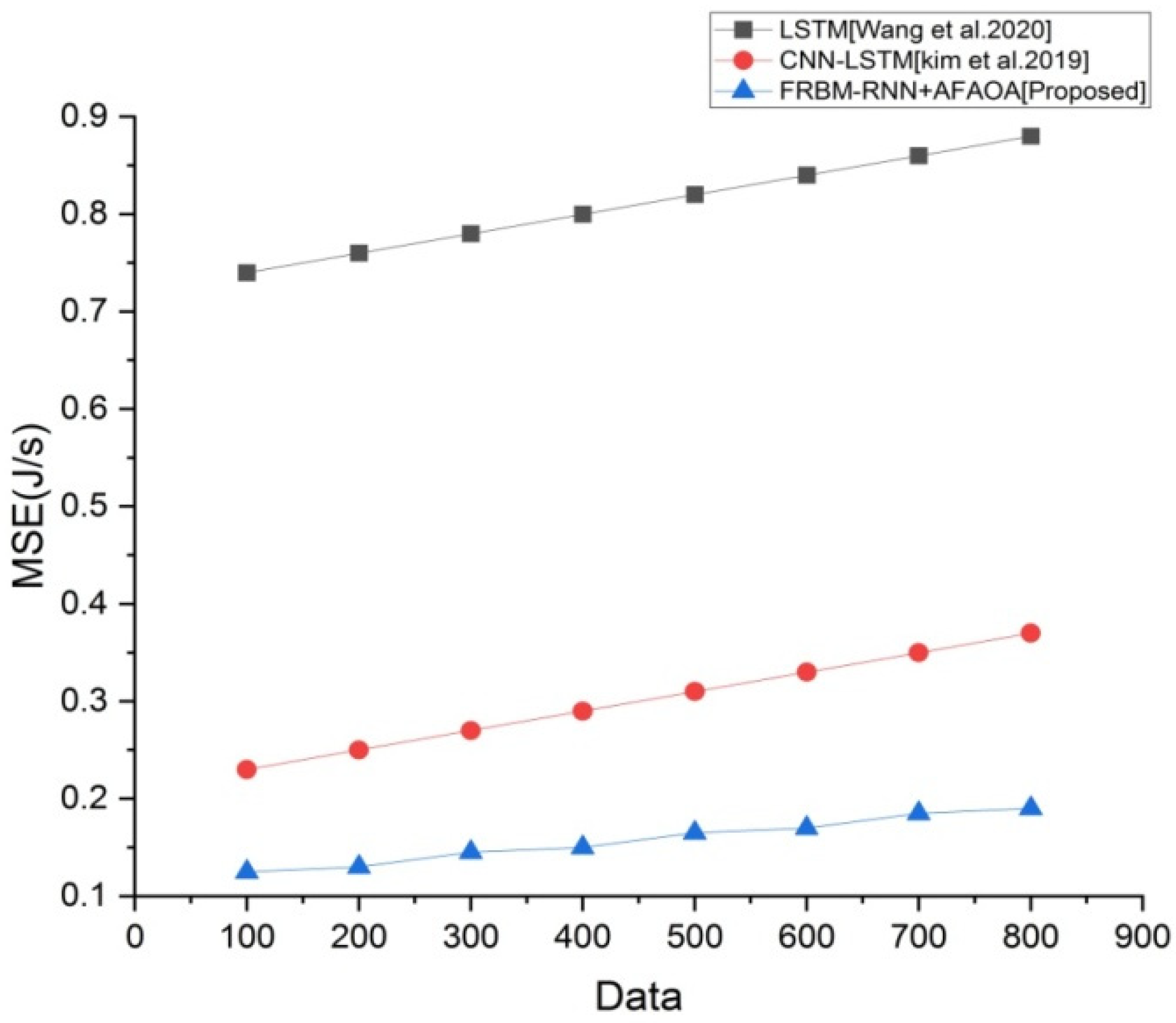
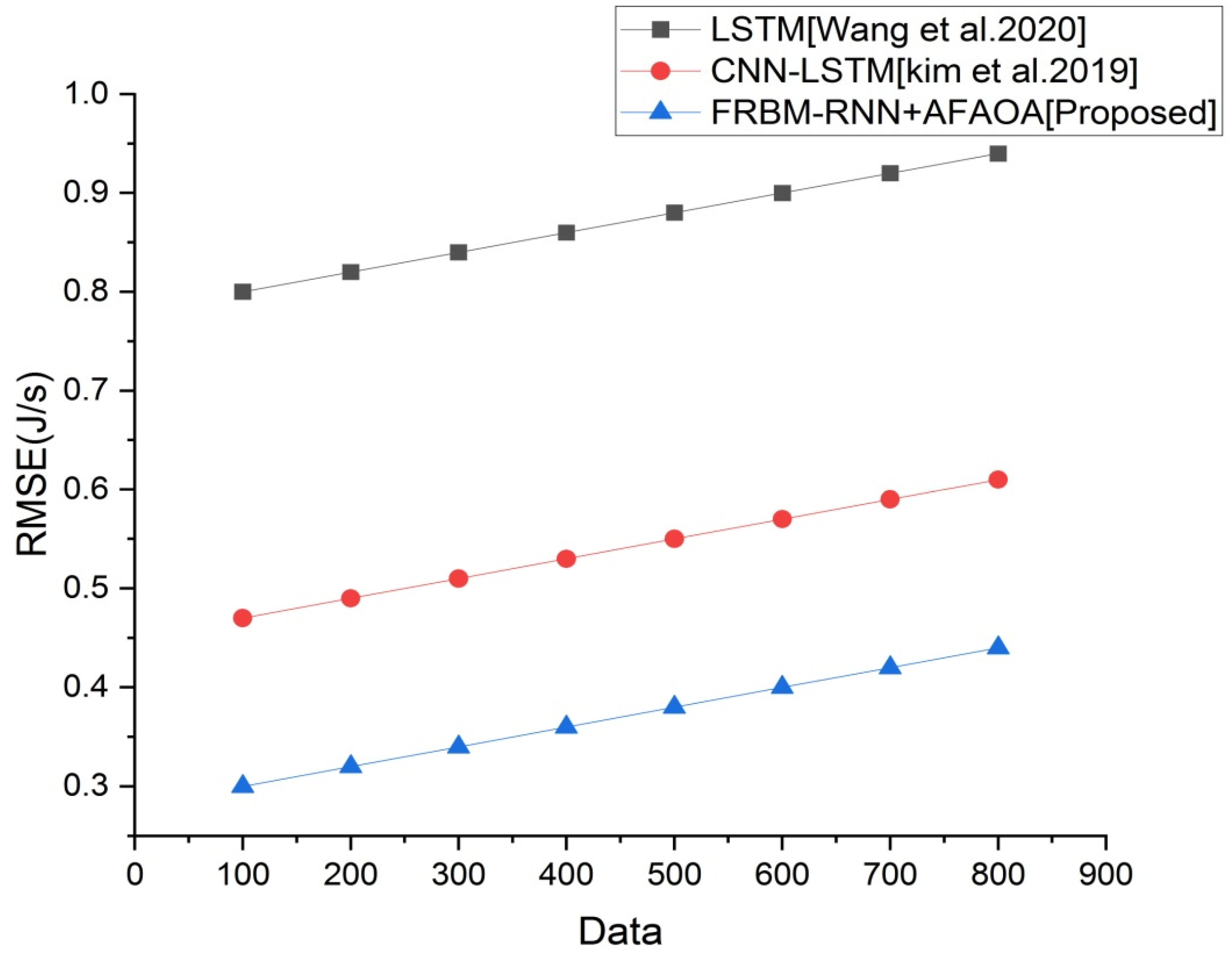
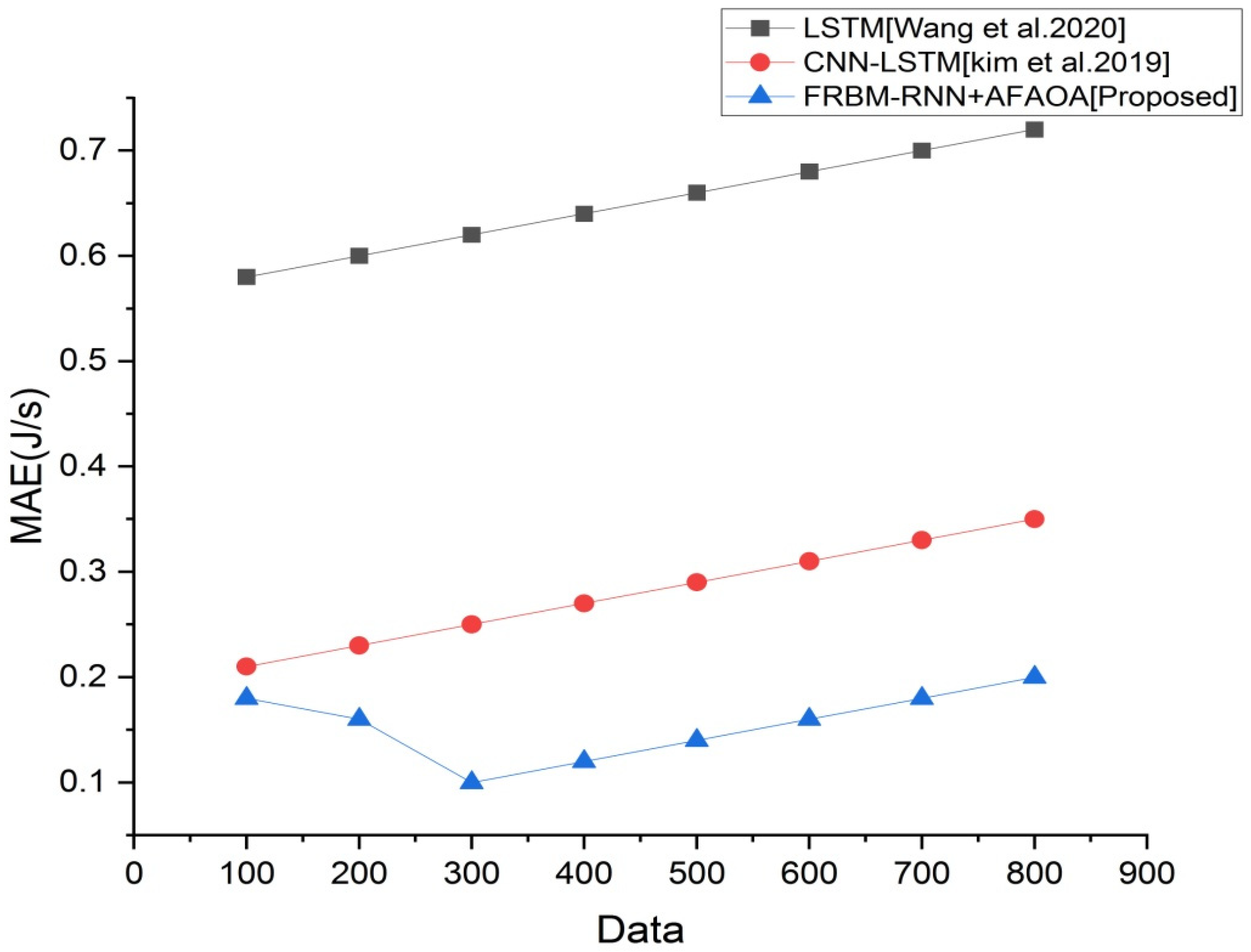
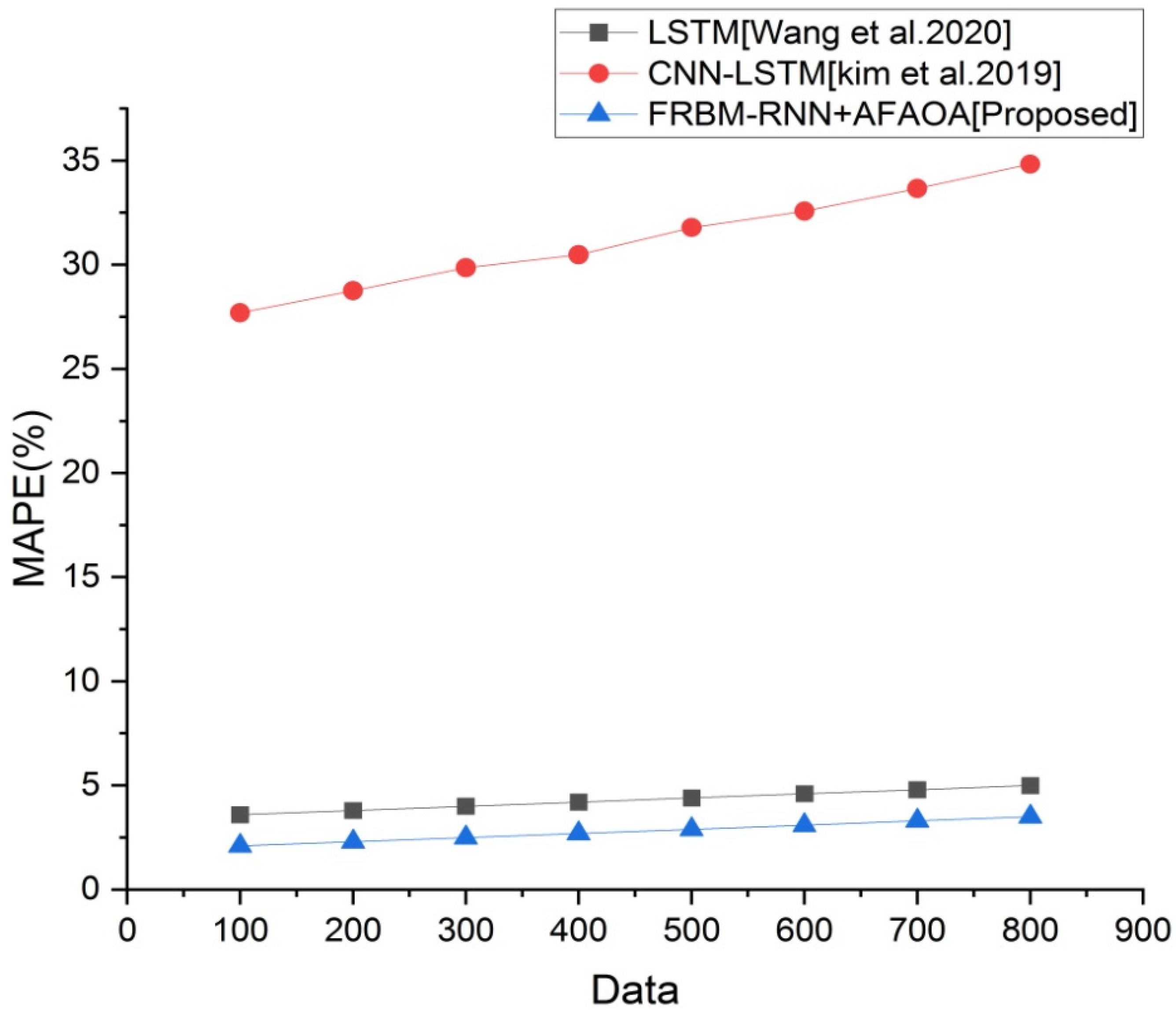
Energy accounting is a system for regularly measuring, analyzing, and reporting the energy use of various activities. This is done to increase energy efficiency and monitor the impact of energy usage on the environment. Primary energy accounting is now done by determining the amount of fossil fuel energy required to generate it. However, if fossil fuels become scarcer, this strategy becomes less viable. Instead, a new energy accounting approach will be required, one that takes into consideration the intermittent character of the two most prevalent renewable energy sources, wind and solar power. Furthermore, estimation of the energy consumption data collected from household surveys, whether using a recall-based approach or a meter-based one, remains a difficult task. Hence, this paper proposes a novel energy accounting model using Fuzzy Restricted Boltzmann Machine-Recurrent Neural Network (FRBM-RNN). The energy consumption dataset is preprocessed using linear-scaling normalization. The proposed model is optimized using the Adaptive Fuzzy Adam Optimization Algorithm (AFAOA). The performance metrics like Mean Square Error (MSE), Root Mean Square Error (RMSE), Mean Absolute Error (MAE), and Mean Absolute Percentage Error (MAPE) are estimated. The estimated results for our proposed technique are MSE (0.19), RMSE (0.44), MAE (0.2), and MAPE (3.5).

1. Introduction

Energy is an essential part of our existence, and practically the whole thing is connected to electricity in some way. The need for electricity is increasing each day. Buildings use a substantial quantity of power globally. Residential energy use has risen, including in the last decade. Building energy consumption accounts for a reliable share of primary energy consumption and is a major contributor to carbon emissions in the world. Emissions of CO₂, air pollution, and global warming are all caused by the usage of energy produced from fossil fuels. According to studies, buildings account for 39 percent of the overall consumption of energy and 38 percent of global ${\mathrm{CO}}_2$ emissions in the world. The major cause for the rise in energy utilization is the developmentof urbanization in recent decades [1].

Building energy use is too high, which is not ideal for a rising country. Depending on the report issued by the Energy Information Administration (EIA) of the US, global energy consumption may rise by 28 percent until 2040. Companies that generate energy are continuously coming under pressure to fulfill the rising energy needs of households and commercial areas. Saving energy (electricity/heating/cooling) is crucial not just for future ecological sustainability, but also for energy businesses and home users. Electricity influences the user’s monthly expenditure, and the client is continually seeking for solutions to save money. To limit energy use and emissions, linked government entities must dedicate major human and financial resources [2].

One of the key aims of countries is to minimize the use of energy and the accompanying emissions of pollutants. The globally known energy-saving plan mandates correct control of energy consumption in residences and the avoidance of unnecessary energy wastage. One of the most crucial components of energy management and operating approaches in constructing resource forecasting models. Precision and powerful energy determination approaches with generalization capability are necessary for successful energy management, planning, and conservation. Energy management and conservation in buildings depend significantly on forecasts, which may aid us in assessing energy consumption, performing building commissioning, and identifying and diagnosing system faults in offices [3].

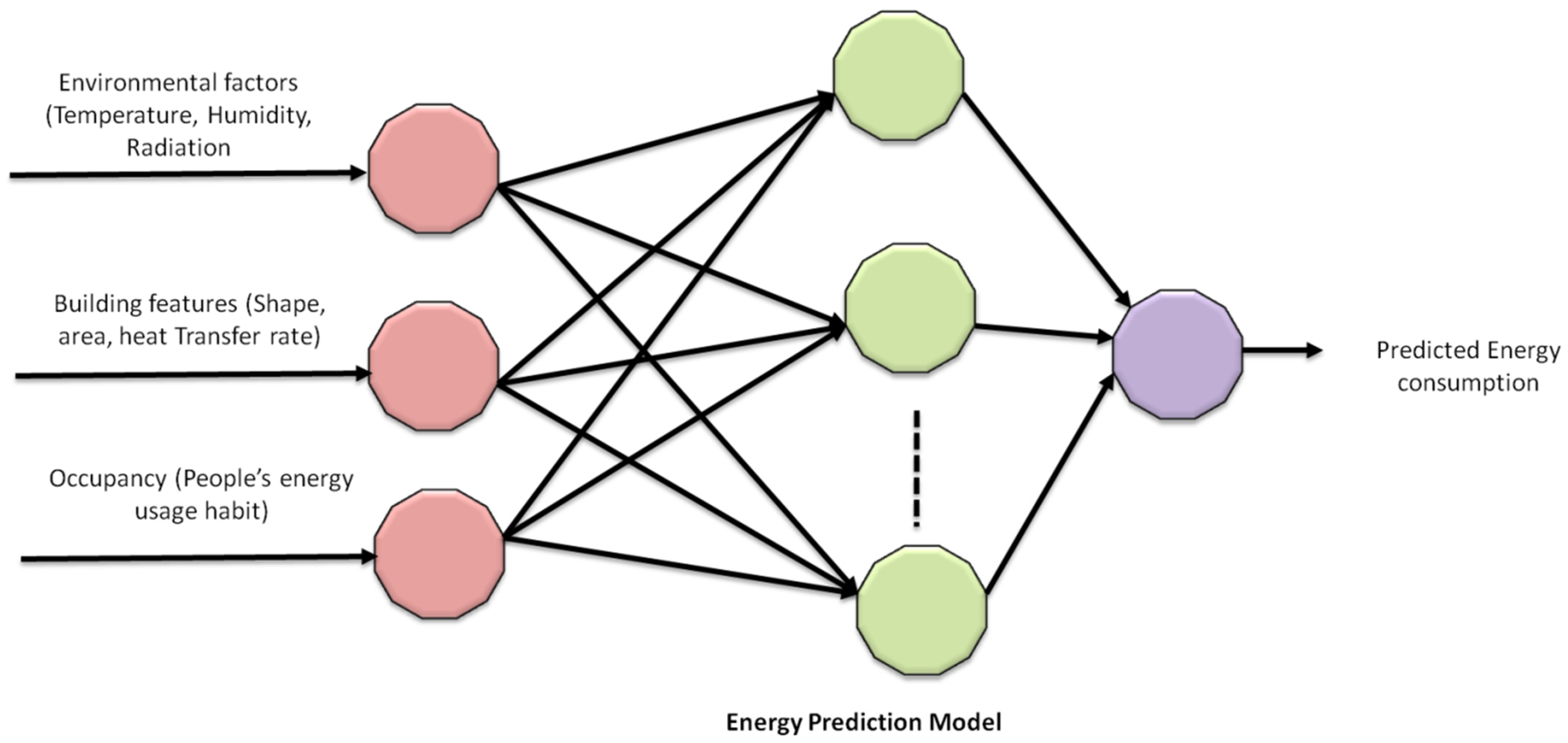
Physical and data-driven models are the basic kinds of energy consumption models. Physical models are not very useful owing to their lesser forecast accuracy. As data mining is revolutionizing many industries, the data-driven approach is presently the most frequent manner owing to the least consumption of time and good performance. These models are useful as they depend on actual data rather than intricate system features. As AI can analyze the data using computer algorithms, data-driven techniques are rapidly being employed in developing energy projections. These models utilize single or hybrid algorithms. These are used to build the relationship between energy usage and other variables. Environmental variables, building features, and occupancy are the three primary forms of inputs for the energy consumption forecast model. Environmental characteristics include indoor and outdoor temperature, relative humidity, and radiation. Occupancy refers to the number of people and their habits of energy use. Building elements include form, size of the building, and heat transfer rate of the wall and roof. Figure 1 displays the various elements that may be given as input to the prediction model. Many scientists have put in a lot of effort and devised numerous ways of estimating energy use [4].

We proposed a novel energy accounting scheme, FRBM-RNN, to determine the energy consumed in buildings in this paper. In addition, the proposed model is optimized using AFAOA to further enhance the prediction accuracy. The major contributions of this paper include:

• To present a novel energy accounting model using Fuzzy Restricted Boltzmann Machine-Recurrent Neural Network (FRBM-RNN).
• To preprocess energy consumption dataset using linear-scaling normalization.
• To optimize the model using the Adaptive Fuzzy Adam Optimization Algorithm (AFAOA).

The remaining sections in the paper are structured as follows. The associated literature and the problem statement are presented in Section 2. The explanations of the proposed work are provided in Section 3. Section 4 has results and discussions. The proposed paper’s conclusion is presented in Section 5.

2. Literature Review

Ref. [5] established a hybrid model that is a hybrid of convolutional neural network (CNN) and long short-term memory (LSTM) to gather spatial and temporal data and estimate dwelling energy use efficiently. The CNN layer helps in extracting features among several factors that influence energy utilization, whereas the LSTM layer is good for training the temporal information of irregular patterns in the components of time series. CNN-LSTM internal analysis was used to reduce the noise in power consumption data, and class activation map was used to examine the factors that have a significant impact on energy consumption prediction. Ref. [6] used an energy usage forecasting system in public buildings to save energy and hence enhance energy efficiency without compromising the comfort level and wellbeing. The ability to estimate energy usage is critical for the operation and planning of intelligent systems. For anticipating such consumption, they utilized an ELM an neural network and a genetic algorithm to maximize the model’s weight. Similarly, the CNN-LSTM main flaw is its complexity, since adding additional components to a neural network—for example, adding a memory layer—increases the connection, resulting in a considerably more complicated model. Ref. [7] illustrated a machine learning baseline model for commercial building energy usage forecast based on the gradient boosting machine (GBM) technique. To increase GBM’s predicted accuracy, they used an extended version of the k-fold validation technique. One possible drawback in practice is that M&V experts are less experienced with machine learning approaches than with traditional regressions. Ref. [8] constructed a mathematical scheme of a Venlo greenhouse’s energy usage depending on the energy conservation concept. Different optimization schemes are utilized to determine the factors in the energy consumption technique that are difficult to calculate. The energy utilization prediction is also challenging to apply to energy predictions in several seasons over the course of a year. Summer cooling energy consumption forecast model has to be investigated further. Ref. [9] suggested a unique technique for estimating periodic energy usage depending on the LSTM network. To begin, the autocorrelation graph is used to extract hidden characteristics from real-world industrial data. Determining the relevant secondary variables as the input to the model is aided by correlation analysis and mechanism analysis. Additionally, the time variable is supplemented to obtain the periodicity more accurately. Many approaches for forecasting energy use have been proposed. Traditional approaches, on the other hand, are ineffective because they do not extract the periodicity concealed in energy use statistics.

Ref. [10] developed a support vector machine energy usage forecasting model to study and assess the energy utilization of hotel structures. The RBF kernel function is chosen as the support vector machine’s kernel function, and the model prediction accuracy is increased by updating the kernel factors. During the modelling process, it was discovered that variables including the flow of people had a significant impact on the hotel’s energy use. For example, a sudden spike in passenger traffic over the holidays may cause the model to become unresponsive. Matching new developments, how to represent the influence of these aspects in the model, and giving hotel managers with a more effective decision-making foundation are all issues that should be addressed in the future. For short-term building energy demand estimation, teaching learning-based optimization (TLBO)was a novel evolutionary strategy adopted by [11]. The original TLBO method is updated in three ways to improve the speed of convergence and accuracy of optimization. To anticipate the electrical energy consumption of different educational institutions, the upgraded technique is combined with artificial neural networks (ANNs). The original TLBO was modified using three steps to speed up convergence and increase optimization accuracy: introducing a review stage, adding an accuracy factor, and deleting the worst solution. Ref. [12] created Hephaestus, a new transfer learning approach for forecasting the energy in buildings depending on time series multi-feature regression with seasonal and trend correction. The suggested technique leverages measurements from other comparable structures gathered over a much longer time period to enhance prediction for an establishing with a limited data set. This technique enables energy prediction by combining data from similar buildings with different distributions and seasonal aspects. For hourly building energy forecast, ref. [13] illustrated a homogeneous ensemble strategy using Random Forest (RF). The method was used to forecast the power demand of two educational facilities in North Central Florida on an hourly basis. Ref. [14] proposed a new method for predictive control depending on the information by buildings utilizing machine learning methods such as regression trees and RF. This method was named the Data-driven model Predictive Control (DPC), and it was used in three studies.

Ref. [15] introduced a unique deep recurrent neural network scheme for predicting the consumption patterns of power in residents and offices for one week at a one-hour resolution. Using real-world building operating data, ref. [16] studied the efficacy of several deep learning approaches in autonomously generating features with high quality for building energy estimation. Convolutional autoencoders, fully connected autoencoders, and generative adversarial networks are applied to create three kinds of deep learning-based features. Ref. [17] developed a unique prediction model known as LSTM with random time effective function (LSTMRT). The effective random time function is employed in LSTM in this case, which takes into account the timeliness of past data as well as the random shift in the market environment. The LSTM model is composed of the properties, namely selected memory and internal time series influence, making it ideal for price time series prediction. For energy demand prediction, ref. [18] suggested a unique neural network-based optimization technique. To begin, the CNN method is used to determine the needed energy demand estimate at the customer level. Second, techniques such as Neural Network-based Particle Swarm Optimization (PSO) and Neural Network-based Genetic Algorithm (NNGA) are utilized to automatically change the neural network weights. Ref. [19] provided a method for estimating occupancy depending on the blind system identification (BSI), as well as a prediction technique for power utilization by air-conditioning machine employing extreme learning machine (ELM),feed-forward neural network (FFNN), and ensemble models.

To more effectively analyze the energy use in residents, ref. [20] introduced a hybrid estimation approach depending on RF and BP neural networks (RF-BPNN). Ref. [21] demonstrated a hybrid deep learning technique that joins an ensemble LSTM neural network with the stationary wavelet transform (SWT) method. The SWT reduces volatility and expands data dimensionality, possibly augmenting the estimation accuracy of LSTM. Furthermore, the suggested method’s predicting performance is improved even further by using an ensemble LSTM neural network. Ref. [22] developed surrogate, zone-level artificial neural networks with occupancy, weather, and internal temperature as input features. A genetic algorithm utilizes them as a validation system to decrease energy usage. Ref. [23] used multiple regression (MLR), multilayer neural network (MNN), RF, and gradient boosting (GB) techniques to design data-driven approaches for determining electricity and consumption of gas in houses. Factors such as economic, demographic, and building attributes were applied as predictors. Ref. [24] suggested a Hidden Markov Model-based approach for predicting energy usage in houses using smart meter data. Ref. [25] introduced an efficient medium and long-term energy determination model depending on machine learning, which included an ANN with an adaptive boosting approach, a nonlinear autoregressive exogenous multivariable input scheme, and a multivariate linear regression technique.

To reflect the full country of Turkey, the forecasting of meteorological data utilized in thermal system design was carried out for 50 cities. Modeling of data acquired from the General Directorate of Meteorology (MGM) was accomplished via the use of artificial neural networks and adaptive-network-based fuzzy inference systems [26].

The approximated temperature values were used to compute the HDD and CDD values for Turkey. To estimate temperature values, an artificial neural network (ANN) and an adaptive network-based fuzzy inference system (ANFIS) were both used. For the feedforward back propagation of the ANN, the Levenberg–Marquardt training method was utilized, but for the ANFIS, the Sugeno-type fuzzy inference method was used [27].

The utilization of energy in buildings is rapidly increasing worldwide. Hence, energy utilization in the building sector must be minimized. The best way to cut down on energy use in an existing structure is to plan and manage the usage of energy strategically. Energy planning, management, and conservation need the use of accurate and robust energy forecast models. Deep learning techniques are gaining importance in designing these models. Hence, we proposed a novel energy accounting scheme, FRBM-RNN, to determine the energy consumed in buildings. The estimation accuracy of the energy utilization prediction strategy which is critical for scheduling and regulating energy use may be improved by enhancing the performance of current algorithms. Therefore, the proposed model is optimized using AFAOA to further enhance the prediction accuracy.

3. Proposed Work

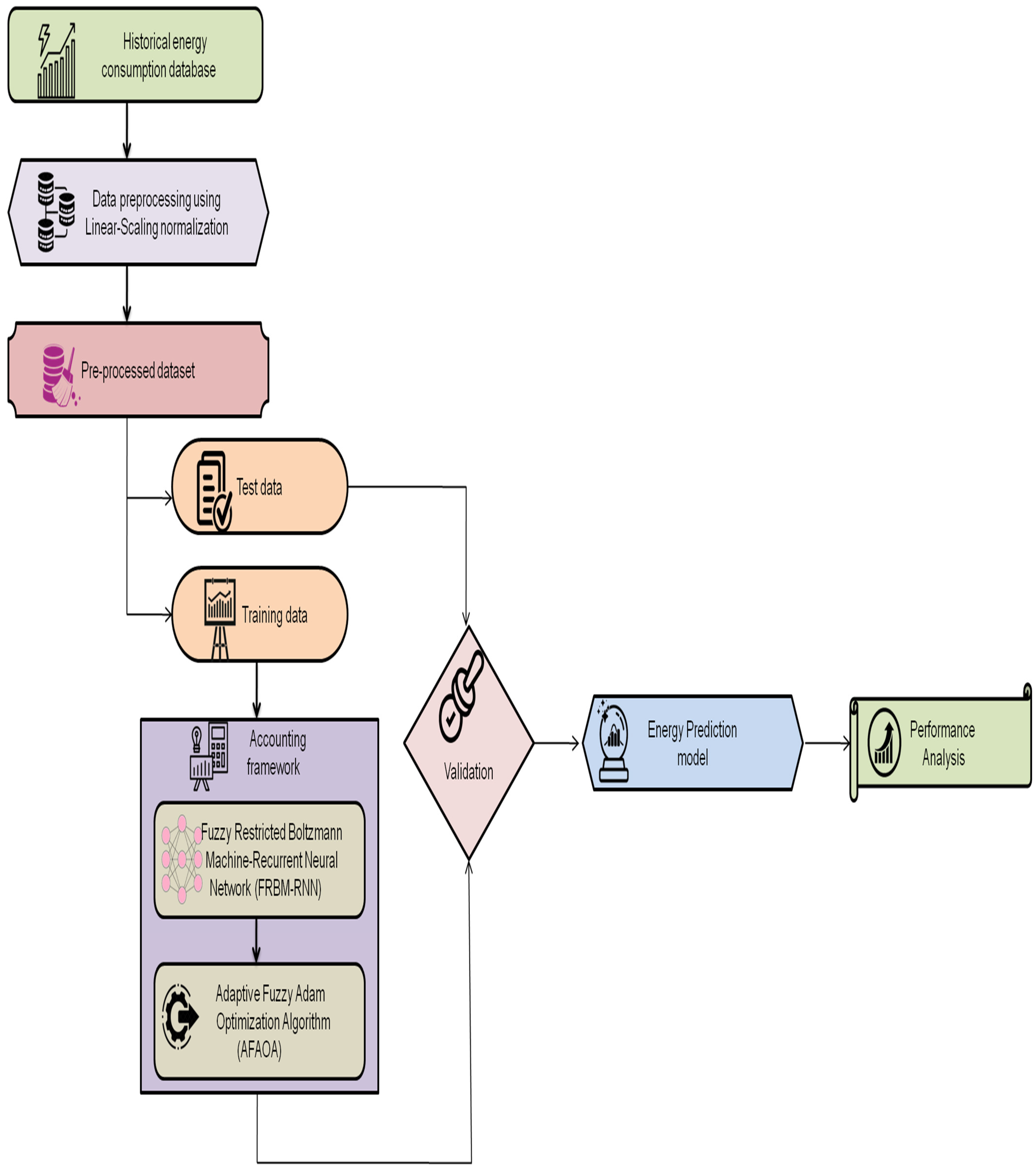
Determination of energy utilization in residential buildings is very important. This paper is focused on designing a new energy accounting model called FRBM-RNN to estimate the energy utilized in buildings. Real-time data is collected and preprocessed using the linear scaling normalization technique. The illustrated model is optimized using AFAOA to improve the predictive performance. The flow of our proposed work is given in Figure 2, and a detailed description is provided in this section.

(a) 

Historical Energy Consumption Database

The dataset for our study was gathered from the library building present in East China. The building includes ten floors with an overall area of 25,542 m² and 13 reading rooms. A full schedule of opening and closing times of the reading rooms was supplied which was considered as the occupancy measure. There is a nearby weather station that collects daily dry-bulb temperatures. Cooling, heating, lighting, ventilation, and plug loads were all taken into account when calculating the building’s energy usage. From 9 October 2009 to 15 January 2010, a total of 2472 time-step data were gathered at hourly intervals [11]

(b) 

Data Preprocessing Using Linear Scaling Normalization (LSN)

Initially, dataset features are preprocessed using LSN. The issue of big number ranges being dominated is avoided by normalizing the dataset’s characteristics, which aids the algorithm in making correct predictions. We obtained the energy consumption data at an hourly resolution. Because of this, a preprocessing strategy was devised to turn the hourly energy consumption data into a maximum linear-scaling transformation. Normalization is used to turn the observed data into values between 0 and 1 across the research period. Next, the scaled hourly data is utilized to represent the average daily energy use. LSN is defined by Equation (1).

$$y_i^{\prime }=\frac{y_i-y_{min}}{y_{max}-y_{min}}$$

(1)

where $y_{min}$ the input dataset’s actual value is $y_{Yi}$ the normalized value scaled according to the range [0,1], _max and _min are the maximum and minimum values of the features, correspondingly. The preprocessed data is categorized into training and testing datasets. Overall, 70% of the preprocessed data are considered as a training set, and the remaining data are noted as a testing set.

(c) 

Fuzzy Restricted Boltzmann Machine-Recurrent Neural Network (FRBM-RNN)

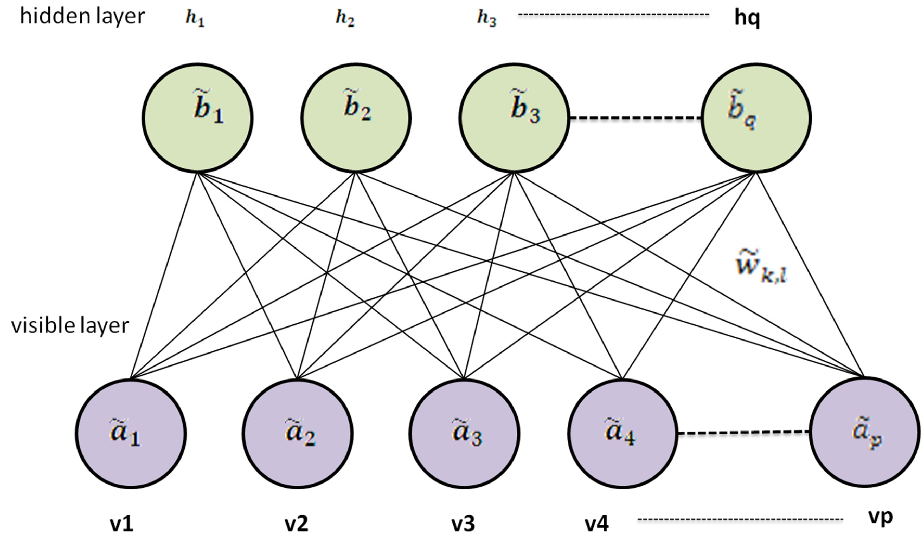
The training dataset is utilized to design the model. The illustrated scheme is a hybrid of FRBM and RNN and it is applied in buildings to determine energy usage. FRBM is advantageous compared to the conventional RBM. FRBM offers greater feature extraction capabilities than standard RBM since the setup parameters are fuzzy. When presented with noisy data, FRBM’s resilience may be improved. Visible and hidden layers are present in FRBM. No connections exist between neurons in the same layer and all connections exist between neurons in other layers. The structure of FRBM is given in Figure 3. The input data are sent to the ‘m’ visible units (v₁, v₂, …, VP), and features of the input data are extracted using ‘n’ hidden layers (h₁, h₂, …, HQ).

The fuzzy energy function, $\tilde{E}\left(v,h,\tilde{\theta }\right)$, is defined by Equation (2).

$$\tilde{E}\left(v,h,\tilde{\theta }\right)=-{\displaystyle \sum }_{k=1}^p{\tilde{a}}_k{v}_k-{\displaystyle \sum }_{l=1}^q{\tilde{b}}_l{h}_l-{\displaystyle \sum }_{k=1}^p{\displaystyle \sum }_{l=1}^q{h}_l{\tilde{w}}_{k,l}{v}_k$$

(2)

where $\tilde{\theta }=\left\{{\tilde{a}}_k,{\tilde{b}}_l, {\tilde{w}}_{k,l}\right\}$ represents fuzzy parameters, ${\tilde{a}}_k$, ${\tilde{b}}_l$, and ${\tilde{w}}_{k,l}$ are fuzzy numbers. ${\tilde{a}}_k$ and ${\tilde{b}}_l$ denote the biases of visible and hidden layers, correspondingly. ${\tilde{w}}_{k,l}$ means the connection weight existing between the kth visible unit and the lth hidden unit. The fuzzy free energy function is simplified into Equation (3).

$$\tilde{G}\left(v\right)=-ln{\displaystyle \sum }_{\overline{h}}{e}^{-\tilde{E}\left(v,h,\tilde{\theta }\right)}=-{\displaystyle \sum }_{k=1}^p{\tilde{a}}_k{v}_k-{\displaystyle \sum }_{l=1}^q\ln \left(1+e^{\left({\tilde{b}}_l+{\displaystyle \sum }_{k=1}^p{\tilde{w}}_{kl}{v}_k\right)}\right)$$

(3)

where $\tilde{G}\left(v\right)$ is the simplified fuzzy energy function.

It is required to use a membership function having higher sensitivity and resolution due to the small size of the parameters and the short fluctuation interval they entail. The symmetric triangle membership function is a great alternative for this purpose. The fuzzy number ${\tilde{a}}_k$ is defined by Equation (4).

$$g_{{\tilde{a}}_k}\left(v\right)=\{\begin{array}{c}0,v\le a_k^L\\ \frac{v-a_k^L}{a_k^M-a_k^L},a_k^L<v<a_k^M\\ \frac{a_k^R-v}{a_k^R-a_k^M},a_k^M<v\le a_k^R\\ 0,v\ge a_k^R\end{array}$$

(4)

where a_k^R, a_k^L, and a_k^M denote the right bound, the left bound, and the center of connection weights, respectively. ${\tilde{b}}_l$, and ${\tilde{w}}_{k,}$ can also be obtained by similar methods.

FRBM’s visible and hidden layers interact best when the parameter is optimally tuned. The objective function becomes nonlinear because the optimum solution is turned into the maximum probability questions regarding fuzzy numbers. That is why figuring out how to compute the fuzzy membership function is so difficult. If the goal function is defuzzified, the issue may be reduced to a calculable maximum likelihood form. Area bisector, the center of centroid, maximum membership, and crisp possibilistic mean value (CPMV) are a few of the defuzzification techniques available.

The function of fuzzy free energy is defuzzified with the help of CPMV. Equation (5) defines the defuzzified free energy function when the membership function is symmetric.

$$\begin{gathered} {\tilde{G}}_s\left(v\right)={{\displaystyle \int }}_0^1\alpha (G^L\left(\alpha \right)+G^R\left(\alpha \right))d\alpha \approx -{\displaystyle \sum }_{k=1}^p\frac{a_k^L+a_k^U}{2}{v}_k-{\displaystyle \sum }_{l=1}^q\frac{\ln \left(1+e^{b_l^L+{{\displaystyle \sum }}_{k=1}^p{W}_{kl}^L{v}_k}\right)}{2} \\ =\frac{1}{2}[-{\displaystyle \sum }_{k=1}^p{a}_k^L{v}_k-{\displaystyle \sum }_{l=1}^q\ln (1+e^{\left(b_R^L+{\displaystyle \sum }_{k=1}^p{W}_{kl}^L{v}_k\right)}-{\displaystyle \sum }_{k=1}^p{a}_k^R{v}_k-{\displaystyle \sum }_{l=1}^q\ln (1+e^{\left(b_R^R+{\displaystyle \sum }_{k=1}^p{W}_{kl}^R{v}_k\right)} \\ =\frac{1}{2}\left[G\left(v,W^L,a^L,b^L\right)+G\left(v,W^R,a^R,b^R\right)\right] \end{gathered}$$

(5)

where ${\tilde{G}}_S\left(V\right)$ represents defuzzified $\tilde{G}\left(v\right)$, G^L(α) and G^R(α) are the left and right boundaries of an interval [G^L(α), G^R(α)], which express the α-cut of the fuzzy number $\tilde{G}\left(\alpha \right)$V.

The probability function of free energy, $P\left(v|\tilde{\theta }\right)$, is provided in Equation (6).

$$P\left(v|\tilde{\theta }\right)=\frac{e^{-{\tilde{G}}_s\left(v\right)}}{{{\displaystyle \sum }}_v{e}^{-{\tilde{G}}_s\left(v\right)}}$$

(6)

The function of negative log-likelihood is defined by Equation (7).

$$\ln N\left(a,\tilde{\theta }\right)=-ln{\displaystyle \prod }_{k=1}^{qr}P\left(v^k|\tilde{\theta }\right)=-{\displaystyle \sum }_{k=1}^{qr}\ln P(\left(v^k|\tilde{\theta }\right)$$

(7)

where is the training data amount? To get the best solution for the parameters according to Equation (8), the stochastic gradient descent approach may be applied to Equation (7).

$$\underset{\tilde{\theta }}{\min }\left(-{\displaystyle \sum }_{v\in r}\ln P(\left(v|\tilde{\theta }\right)\right)$$

(8)

The partial derivatives of $\ln (\left(v|\tilde{\theta }\right)$ are computed. Contrastive Divergence is used to approximate the partial derivatives of the maximum log-likelihood gradient to simplify the complexity of computation. The significant features for estimating energy usage are collected from the hidden layers of FRBM.

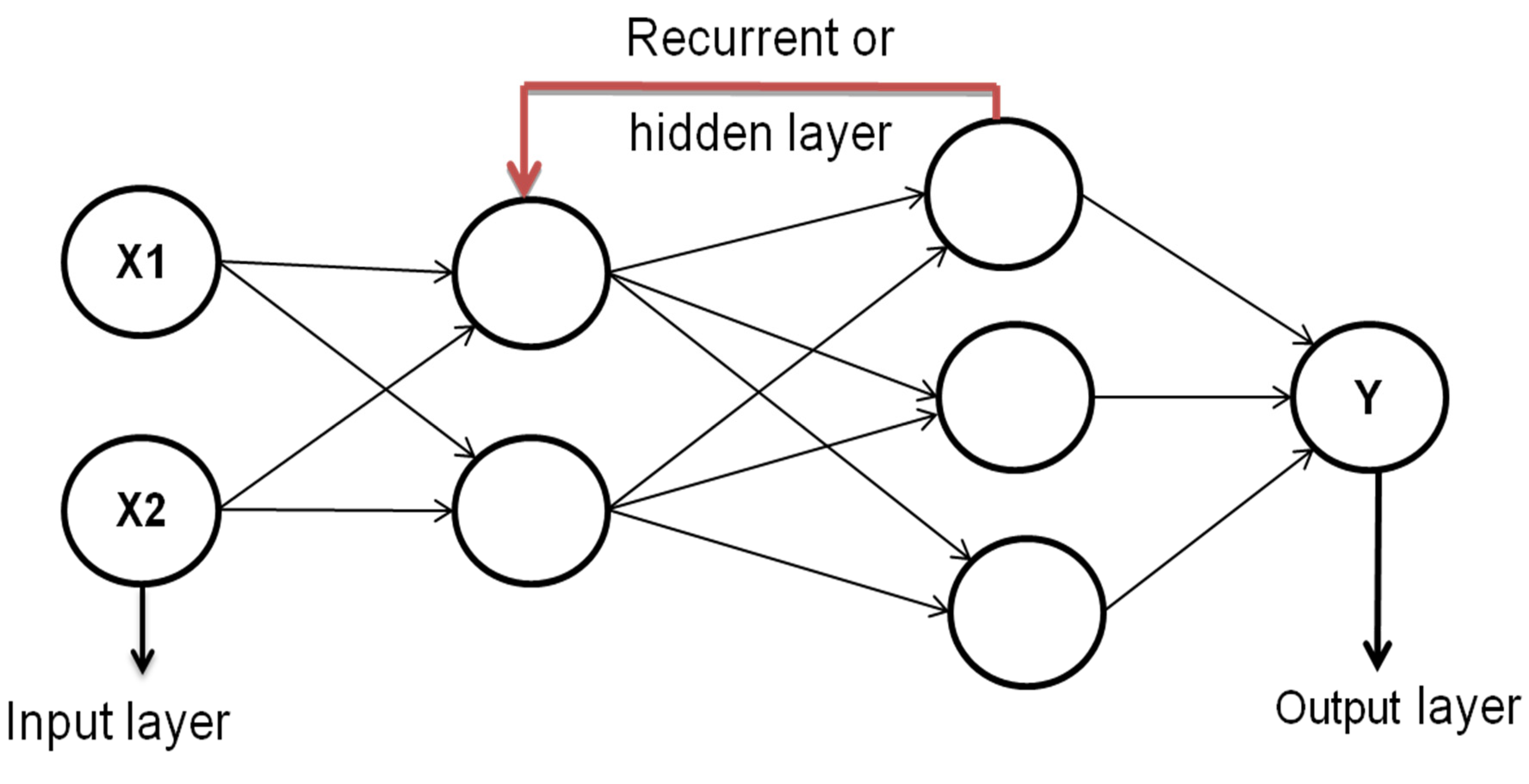
The extracted features from FRBM are sent to RNN for determining the energy. In their hidden layers, RNNs differ from basic feed-forward neural networks. RNN hidden layers are fed not only by the inputs from their preceding layer but also by the initiations of themselves for the previous inputs that they receive. Nodes in the hidden layer of RNN are linked to the prior activation of all the other hidden layers. It is the activation functions of the RNN that determine the neuron’s output level, and the RNN has several inputs. The RNN process is based on a forward and backward pass, respectively. The input, hidden, and output layers are included in RNN, and its architecture is depicted in Figure 4.

Here, we are training the RNN based on the available energy dataset and extracted features. The inputs for the input layer are initialized and the weights are assigned to them. The RNN’s forward pass is given in Equation (9).

$${\gamma }_c\left(m\right)={\displaystyle \sum }_d{\delta }_d\left(m\right)w_{cd}\left(m\right)$$

(9)

where ${\gamma }_c$ is the input neuron and W_cd is the value of the assigned weight. ${\delta }_c$ is the neuron’s activation state at a time ‘m’ according to Equation (10).

$${\delta }_c\left(m\right)=f_c\left({\gamma }_c\left(m\right)\right)$$

(10)

where c = 1,2,….

According tothe network inputs, activation function fc is determined. Based on the activation functions, the functions of hidden node are constructed. The activation function of unseen nodesis processed through sigmoid function to derive decision vector. Each neuron’s backward pass output is computed using the function specified in Equation (11).

$${\delta }_c\left(m\right)=f_c\left({\gamma }_c\left(m\right),C_c\left(m\right)\right)$$

(11)

$${\gamma }_c\left(m\right)={\displaystyle \sum }_{d\in h}{\delta }_d\left(m\right)w_{cd}+{\displaystyle \sum }_{d\in i}{\gamma }_d\left(m\right)w_{cd}+{\displaystyle \sum }_{d\in C}{\delta }_d\left(m-{\tau }_{cd}\right)w_{cd}$$

(12)

where i and h denote the values of input neurons and hidden layer, correspondingly, the neuron’s value C reflects the previous network stage’s data stored in the neuron’s memory, ${\delta }_d$ means the dth input neuron, and ${\tau }_{cd}$ denotes an integer value that represents the dislocation in recurrent network occurred in a given period. Backpropagation through time delay (BPTT) and Bayesian regulation (BR)are used to train the RNN. The backpropagation error, ${\mu }_h$, is determined by Equation (13).

$${\mu }_h={\delta }^t-\widehat{\delta }$$

(13)

The BR approach may reduce the error. The BR approach is employed to train the neural network at this moment. By combining the average total of squared network errors and weights, this BR approach develops a better-utilized network by selecting the correct amalgamation. The weight and bias values are adjusted by Equation (14) using the BR approach, which is a function of network training and based on Levenberg–Marquardt optimization.

$${\mu }_d=\frac{1}{Q}{\displaystyle \sum }_{c=1}^Q\left({\left({\mu }_h\right)}^2\right)$$

(14)

where ${\mu }_d$ is the network’s updated weight.

The network’s weights are updated finally. The output of the trained RNN is the predicted energy consumption.

(d) 

Adaptive Fuzzy Adam Optimization Algorithm (AFAOA)

AFAOA speeds up the learning process and increases the machine’s efficiency by allowing the planned model to converge more quickly. AFAOA is a stochastic optimization algorithm applied to optimize the features for enhancing the training process of FRBM-RNN. The AFAOA is a modified variation of stochastic gradient descent (SGD) that has lately gained popularity in deep learning applications. The weights of RNN can be updated repeatedly depending on training data. The important formulas to define the optimization process using AFAOA are provided in Equations (15)–(20).

$$g_z={\nabla }_{\theta }{f}_z({\theta }_{z-1)}$$

(15)

$$h_z={\beta }_1.h_{z-1}+\left(1-{\beta }_1\right).g_z$$

(16)

$$v_z={\beta }_2.v_{z-1}+\left(1-{\beta }_2\right).g_z^2$$

(17)

$${\widehat{h}}_z=\frac{h_z}{1-{\beta }_1^z}$$

(18)

$${\widehat{v}}_z=\frac{v_z}{1-{\beta }_2^z}$$

(19)

$${\theta }_z={\theta }_{z-1}-\frac{\alpha .\widehat{h_z}}{\sqrt{\widehat{v_z}}+\epsilon }$$

(20)

where $\alpha$ means the size of the step, β₁ and β₂ represent the exponential decay rates, and z denotes the time-step. f($\theta$) denotes the stochastic objective function, ${\theta }_0$ and ${\theta }_z$ represent the initial and final parameter vectors, respectively, h_z and v_z denote first and second-moment vectors, respectively, ${\widehat{\theta }}_{Hz}$ and ${\widehat{v}}_z$ are bias-corrected moment estimates, and $g_z^2$ means the element-wise square.

Initially, the step size, exponential decay rates, and objective function are confirmed. The parameter vector, first and second-moment vectors, and time-step are initialized. Then, the loop’s every part is repeatedly updated until the parameter ${\theta }_z$ converges. The stochastic objective function is renewed at the time-step ‘z’. The biased first and second moments were estimated. Then, the bias-corrected first and second-moment estimates were calculated. Finally, the parameters of RNN were updated using the above-determined value. The prediction performance of the optimized FRBM-RNN using AFAOA is evaluated against the testing set.

4. Results and Discussion

This work focuses on the design of FRBM-RNN and its optimization using AFAOA to accurately anticipate the energy usage in buildings. The testing set was used to ensure that FRBM-RNN+AFAOA was accurate. Our model was compared to the existing techniques such as CNN-LSTM and LSTM. The performance metrics utilized for the model’s validation are RMSE, MAE, MSE, and MAPE. The simulation results were generated using MATLAB.

MSE is defined as the variations between the determined and actual energy consumption. It is calculated by Equation (21). It is measured in joule per second (J/s).

$$MSE=\frac{1}{n}{\displaystyle \sum }_{i=1}^n{\left(T_{O,i}-T_{P,i}\right)}^2$$

(21)

where T_O is the actual value and T_p is the determined value of energy consumed, n represents the sample size and i = 1 to n.

RMSE means the square root of MSE and it is defined in Equation (22). It is measured in joule per second (J/s).

$$RMSE=\sqrt{\frac{{{\displaystyle \sum }}_{i=1}^n{\left(T_{O,i}-T_{P,i}\right)}^2}{n}}$$

(22)

MAE is described as the average of the absolute values of the prediction errors. It is determined by Equation (23). It is measured in joule per second (J/s).

$$MAE=\frac{1}{n}{\displaystyle \sum }_{i=1}^n\left|T_{O,i}-T_{P,i}\right|$$

(23)

MAPE is the mean of the absolute percentage errors of prediction and is defined by Equation (24). It is measured in percentage (%).

$$MAPE=\frac{100}{n}{\displaystyle \sum }_{i=1}^n\left|\frac{T_{O,i}-T_{P,i}}{T_{P,i}}\right|$$

(24)

Coefficient of variation (COV) is defined as the standard deviation divided by the mean and multiplied by 100. Additionally, it is determined by Equation (25):

$$COV=\frac{S}{\overline{X}}\ast 100$$

(25)

S is the standard deviation and $\overline{X}$ is the mean.

It is shown in Figure 5 that FRBM-RNN+AFAOA exhibited lower MSE when compared to LSTM and CNN-LSTM. If the value of MSE is lower, the determination performance of the approach is better. From Figure 6, it is clear that the RMSE value of our suggested model is lesser than that of CNN-LSTM and LSTM. This confirms that FRBM-RNN+AFAOA showed a lesser prediction error. MAE value of our suggested model was lesser compared to the existing methods. This was observed in Figure 7. The lesser MAE value of FRBM-RNN+AFAOA illustrated that the deviation of predicted building energy from the actual building energy was not so much. In addition, this result shows that the energy predicted by the model was very closer to the actual energy utilized in the buildings. From Figure 8, it is clear that our suggested technique exhibited lower MAPE when compared to CNN-LSTM and LSTM. This confirms that the FRBM-RNN+AFAOA method achieved higher prediction accuracy.

Table 1. Comparative analysis of prediction performance.

Methods	MSE	RMSE (J per s)	MAE	MAPE	COV
FRBM-RNN + AFAOA (proposed)	0.19	0.44	0.2	3.5	0.15
CNN-LSTM [5]	0.37	0.61	0.35	34.84	0.29
LSTM [9]	0.88	0.94	0.72	5	0.66

showed the performance analysis of the different methods. Combining the benefits of Convolutional neural networks (CNN) that can obtain effective features from the data, and long short-term memory (LSTM), which could not only search the interdependence of data in time series data, but also automatically detect the best mode appropriate for relevant data while comparing with the FRBM-RNN+AFAO. Figure 9 shows the comparative analysis of different models based on COV. From the figure it is clear that the proposed method has a lower COV than the conventional approaches. From the analysis of these results, it is confirmed that our proposed model determines the energy consumed in the buildings accurately and efficiently compared to CNN-LSTM and LSTM.

5. Discussion

In many practical systems, energy consumption data is a kind of time–series data with periodicity, but standard forecasting approaches ignore periodicity. Ref. [9] provide a unique technique for estimating periodic energy usage based on a CNN-LSTM (Long short-term memory) network. The autocorrelation graph extracts hidden patterns from actual industrial data. Finding the relevant secondary variables as model input is aided by correlation coefficient and mechanism analysis. Due to its significant economic benefits, the work of energy forecasting has taken on a significant role in our everyday lives. Many approaches for forecasting energy use have been proposed. Traditional approaches, on the other hand, are ineffective because they do not extract the periodicity concealed in energy use statistics. In today’s world, the fast increase in the population and technological advancements have dramatically increased electricity consumption. As electricity is used at the same time as it is created at the power station, precise forecasting of energy consumption is critical for reliable power supply. Finally, using CNN-LSTM internal analysis, we validated the process of decreasing noise in power consumption data and investigated the factors that have a significant impact on energy consumption prediction using a class activation map. The CNN-LSTM model developed in this work predicts irregular electrical energy usage patterns that are not anticipated by current machine learning approaches. When compared to existing methods, the proposed method provides better results.

6. Conclusions

Prediction of energy consumed in buildings has become a crucial part of our everyday lives due to the rise in energy demand worldwide. This could support the energy managers to plan and manage the energy efficiency in buildings and conserve the energy in the world. Therefore, the development of accurate models for predicting energy use is of tremendous importance. In this paper, we proposed the FRBM-RNN technique to estimate the energy utilized in buildings. In addition, the AFAOA approach was applied to augment the estimation performance of the FRBM-RNN model. The performance of the proposed model was compared with the existing techniques namely CNN-LSTM and LSTM. FRBM-RNN+AFAOA strategy exhibited lower MSE, RMSE, MAE, and MAPE values compared to the conventional methods. This confirmed that the estimation of energy consumed in the buildings using our proposed model was highly accurate and consistent. The limitations are Gradient explosion and disappearing difficulties are challenges with recurrent neural networks. It is quite difficult to train an RNN. When Tan h or Relu is used as an activation feature, it cannot handle exceedingly long sequences. Large amounts of training data are required, as the position of objects is not encoded in CNN-LSTM.

In the future, this study can be embedded into the smart grids of other building categories to forecast energy consumption.

References

- Zhong, H.; Wang, J.; Jia, H.; Mu, Y.; Lv, S. Vector field-based support vector regression for building energy consumption prediction. Appl. Energy 2019, 242, 403–414. [Google Scholar] [CrossRef]
- Fayaz, M.; Kim, D. A prediction methodology of energy consumption based on a deep extreme learning machine and comparative analysis in residential buildings. Electronics 2018, 7, 222. [Google Scholar] [CrossRef]
- Wang, R.; Lu, S.; Li, Q. A multi-criteria comprehensive study on a predictive algorithm of hourly heating energy consumption for residential buildings. Sustain. Cities Soc. 2019, 49, 101623. [Google Scholar] [CrossRef]
- Bourdeau, M.; Qiang Zhai, X.; Nefzaoui, E.; Guo, X.; Chatellier, P. Modeling and forecasting building energy consumption: A review of data-driven techniques. Sustain. Cities Soc. 2019, 48, 101533. [Google Scholar] [CrossRef]
- Kim, T.Y.; Cho, S.B. Predicting residential energy consumption using CNN-LSTM neural networks. Energy 2019, 182, 72–81. [Google Scholar] [CrossRef]
- Ruiz, L.G.B.; Rueda, R.; Cuéllar, M.P.; Pegalajar, M.C. Energy consumption forecasting based on Elman neural networks with evolutive optimization. Expert Syst. Appl. 2018, 92, 380–389. [Google Scholar] [CrossRef]
- Touzani, S.; Granderson, J.; Fernandes, S. Gradient boosting machine for modeling the energy consumption of commercial buildings. Energy Build. 2018, 158, 1533–1543. [Google Scholar] [CrossRef] [Green Version]
- Shen, Y.; Wei, R.; Xu, L. Energy consumption prediction of a greenhouse and optimization of daily average temperature. Energies 2018, 11, 65. [Google Scholar] [CrossRef] [Green Version]
- Wang, J.Q.; Du, Y.; Wang, J. LSTM-based long-term energy consumption prediction with periodicity. Energy 2020, 197, 117197. [Google Scholar] [CrossRef]
- Shao, M.; Wang, X.; Bu, Z.; Chen, X.; Wang, Y. Prediction of energy consumption in hotel buildings via support vector machines. Sustain. Cities Soc. 2020, 57, 102128. [Google Scholar] [CrossRef]
- Li, K.; Xie, X.; Xue, W.; Dai, X.; Chen, X.; Yang, X. A hybrid teaching-learning artificial neural network for building electrical energy consumption prediction. Energy Build. 2018, 174, 323–334. [Google Scholar] [CrossRef]
- Ribeiro, M.; Grolinger, K.; ElYamany, H.F.; Higashino, W.A.; Capretz, M.A. Transfer learning with seasonal and trend adjustment for cross-building energy forecasting. Energy Build. 2018, 165, 352–363. [Google Scholar] [CrossRef]
- Wang, Z.; Wang, Y.; Zeng, R.; Srinivasan, R.S.; Ahrentzen, S. Random Forest-based hourly building energy prediction. Energy Build. 2018, 171, 11–25. [Google Scholar] [CrossRef]
- Smarra, F.; Jain, A.; De Rubeis, T.; Ambrosini, D.; D’Innocenzo, A.; Mangharam, R. Data-driven model predictive control using random forests for building energy optimization and climate control. Appl. Energy 2018, 226, 1252–1272. [Google Scholar] [CrossRef] [Green Version]
- Rahman, A.; Srikumar, V.; Smith, A.D. Predicting electricity consumption for commercial and residential buildings using deep recurrent neural networks. Appl. Energy 2018, 212, 372–385. [Google Scholar] [CrossRef]
- Fan, C.; Sun, Y.; Zhao, Y.; Song, M.; Wang, J. Deep learning-based feature engineering methods for improved building energy prediction. Appl. Energy 2019, 240, 35–45. [Google Scholar] [CrossRef]
- Yang, Y.; Wang, J.; Wang, B. Prediction model of the energy market by long short-term memory with random system and complexity evaluation. Appl. Soft Comput. 2020, 95, 106579. [Google Scholar] [CrossRef]
- Muralitharan, K.; Sakthivel, R.; Vishnuvarthan, R. Neural network-based optimization approach for energy demand prediction in smart grid. Neurocomputing 2018, 273, 199–208. [Google Scholar] [CrossRef]
- Wei, Y.; Xia, L.; Pan, S.; Wu, J.; Zhang, X.; Han, M.; Zhang, W.; Xie, J.; Li, Q. Prediction of occupancy level and energy consumption in an office building using blind system identification and neural networks. Appl. Energy 2019, 240, 276–294. [Google Scholar] [CrossRef]
- Zhang, X.; Zhang, J.; Zhang, J.; Zhang, Y. Research on the Combined Prediction Model of Residential Building Energy Consumption Based on Random Forest and BP Neural Network. Geofluids 2021, 2021, 7271383. [Google Scholar] [CrossRef]
- Yan, K.; Li, W.; Ji, Z.; Qi, M.; Du, Y. A hybrid LSTM neural network for energy consumption forecasting of individual households. IEEE Access 2019, 7, 157633–157642. [Google Scholar] [CrossRef]
- Reynolds, J.; Rezgui, Y.; Kwan, A.; Piriou, S. A zone-level, building energy optimization combining an artificial neural network, a genetic algorithm, and model predictive control. Energy 2018, 151, 729–739. [Google Scholar] [CrossRef]
- Gassar, A.A.A.; Yun, G.Y.; Kim, S. A data-driven approach to the prediction of residential energy consumption at urban scales in London. Energy 2019, 187, 115973. [Google Scholar] [CrossRef]
- Ullah, I.; Ahmad, R.; Kim, D. A prediction mechanism of energy consumption in residential buildings using a hidden Markov model. Energies 2018, 11, 358. [Google Scholar] [CrossRef] [Green Version]
- Ahmad, T.; Chen, H. Potential of three variant machine-learning models for forecasting district-level medium-term and long-term energy demand in a smart grid environment. Energy 2018, 160, 1008–1020. [Google Scholar] [CrossRef]
- Işık, E.; Inallı, M. Artificial neural networks and adaptive neuro-fuzzy inference systems approach to forecasting the meteorological data for HVAC: The case of cities for Turkey. Energy 2018, 154, 7–16. [Google Scholar] [CrossRef]
- Işık, E.; İnallı, M.; Celik, E. ANN and ANFIS approach to calculate the heating and cooling degree day values: The case of provinces in Turkey. Arab. J. Sci. Eng. 2019, 44, 7581–7597. [Google Scholar] [CrossRef]
Figure 1.
General design of energy prediction model [Source: Author].
Figure 2.
Flow of the proposed work [Source: Author].
Figure 3.
Structure of FRBM [Source: Author].
Figure 4.
Framework of RNN [Source: Author].
Figure 5.
Graphical analysis of different models based on MSE [Source: Author].
Figure 6.
Graphical analysis of various models based on RMSE [Source: Author].
Figure 7.
Graphical analysis of different methods based on MAE [Source: Author].
Figure 8.
Graphical analysis of various methods depending on MAPE [Source: Author].
Figure 9.
Graphical analysis of various methods depending on COV [Source: Author].
Disclaimer/Publisher’s Note: The statements, opinions and data contained in all publications are solely those of the individual author(s) and contributor(s) and not of MDPI and/or the editor(s). MDPI and/or the editor(s) disclaim responsibility for any injury to people or property resulting from any ideas, methods, instructions or products referred to in the content. |
© 2023 by the authors. Licensee MDPI, Basel, Switzerland. This article is an open access article distributed under the terms and conditions of the Creative Commons Attribution (CC BY) license (https://creativecommons.org/licenses/by/4.0/).
Share and Cite
MDPI and ACS Style
Sorguli, S.; Rjoub, H. A Novel Energy Accounting Model Using Fuzzy Restricted Boltzmann Machine—Recurrent Neural Network. Energies 2023, 16, 2844. https://doi.org/10.3390/en16062844
AMA Style
Sorguli S, Rjoub H. A Novel Energy Accounting Model Using Fuzzy Restricted Boltzmann Machine—Recurrent Neural Network. Energies. 2023; 16(6):2844. https://doi.org/10.3390/en16062844
Chicago/Turabian StyleSorguli, Sarhang, and Husam Rjoub. 2023. "A Novel Energy Accounting Model Using Fuzzy Restricted Boltzmann Machine—Recurrent Neural Network" Energies 16, no. 6: 2844. https://doi.org/10.3390/en16062844
Note that from the first issue of 2016, this journal uses article numbers instead of page numbers. See further details here.