Open-Source Energy, Entropy, and Exergy 0D Heat Release Model for Internal Combustion Engines

Abstract

Internal combustion engines face increased market, societal, and governmental pressures to improve performance, requiring researchers to utilize modeling tools capable of a thorough analysis of engine performance. Heat release is a critical aspect of internal combustion engine diagnostic analysis, but is prone to variability in modeling validity, particularly as engine operation is pushed further from conventional combustion regimes. To that end, this effort presents a comprehensive open-source, zero-dimensional equilibrium heat release model. This heat release analysis is based on a combined mass, energy, entropy, and exergy formulation that improves upon well-established efforts constructed around the ratio of specific heats. Furthermore, it incorporates combustion using an established chemical kinetics mechanism to endeavor to predict the global chemical species in the cylinder. Future efforts can augment and improve the chemical kinetics reactions for specific combustion conditions based on the radical pyrolysis of the fuel. In addition, the incorporation of theoretical calculations of energy and exergy based on the change in chemical species allows for cross-checking of combustion model validity.

1. Introduction

In the current era, the internal combustion engine (ICE) faces considerable pressure to improve performance and lower emissions, requiring proper tools for quantifying and illustrating engine performance metrics from measured data. The root of ICE performance analysis is diagnostic rate of heat release (RHR) modeling, which utilizes the in-cylinder pressure trace to allow for proper accounting of the pathways through which thermal energy from combustion is alternatively used for work or lost to the surrounding environment [1].

The standard methodology for quantifying heat release is as presented in Heywood [1]. This method originates from the open system energy equation and utilizes in-cylinder pressure data recorded during the compression and expansion strokes:

$$\frac{dQ}{dt}-p\frac{d{V}_{\mathrm{CV}}}{dt}+{\displaystyle \sum _{in}{\dot{m}}_{in}{h}_{in}}=\frac{d{U}_{\mathrm{CV}}}{dt}$$

(1)

where dQ/dt is the rate of total heat transfer into the system through its boundary, p⋅dV_CV/dt is the rate of boundary work completed by the moving piston, ${\dot{m}}_{in}$ is the mass flow rate entering the system through the system boundary, h_in is the enthalpy of the mass entering the system, and dU_CV/dt is the rate of change in the total energy of the mass contained in the system. For direct-injection engines, Equation (1) is rewritten as follows:

$$\frac{dQ}{dt}-p\frac{d{V}_{\mathrm{CV}}}{dt}+{\dot{m}}_f{h}_f=\frac{d{U}_{\mathrm{CV}}}{dt}$$

(2)

where the _𝑓 subscript denotes fuel. Considering U as the sensible internal energy of the contents within the cylinder and h_f as the injected fuel, sensible enthalpy helps distinguish dQ/dt as the difference between the energy (aka heat) released through chemical combustion and the rate of heat transfer. Hence, the apparent heat release rate (dQ/dt) is indicated through a gross rate of heat release (dQ_HR/dt) and the heat transfer rate to and from the walls and piston (dQ_HT/dt); here, heat transfer is defined as negative when leaving the cylinder. This must equal the sum of the rate of change of sensible internal energy of the system and the piston work as follows:

$$\frac{dQ}{dt}=\frac{d{Q}_{HR}}{dt}+\frac{d{Q}_{HT}}{dt}=\frac{d{U}_{\mathrm{CV}}}{dt}+p\frac{d{V}_{\mathrm{CV}}}{dt}-{\dot{m}}_f{h}_f$$

(3)

Assuming the cylinder contents behave like ideal gases with a constant gas constant (R), Equation (3) is further reduced to the following:

$$\frac{dQ}{dt}=\left(\frac{k}{k-1}\right)p\frac{d{V}_{\mathrm{CV}}}{dt}+\left(\frac{1}{k-1}\right)V_{\mathrm{CV}}\frac{dp}{dt}$$

(4)

where k is the ratio of the specific heats with usual values ranging between 1.30 and 1.35 for single-zone compression ignition (CI) combustion models. Sometimes, for better accuracy, k is taken as 1.35 at the end of the compression stroke and 1.26–1.30 at the overall equivalence ratio following combustion. However, the appropriate values for k during combustion are not well-defined, primarily owing to (a) the quasi-static nature of the fuel injection, atomization, vaporization, and mixing processes; (b) the instantaneously indeterminable composition of burned gases; (c) the accuracy of the available heat transfer correlations; and (d) heat loss through crevices. These phenomena must be determined accurately to develop better heat release models at the cost of complexity and greater computational costs. For this model, the influence of chemical species changing throughout the entire combustion process comes down to the single parameter k.

Beyond the core model, numerous variations exist to expand on the core of heat release modeling to address individual research interests [2]. From a modeling standpoint, the most prevalent work involves improving the determination of the combustion rate and ignition timing based on a combination of measured operational data and empirical combustion models (e.g., the Wiebe function) [3,4]. Significant work is also associated with the expansion of heat release modeling to include alternative fuels, particularly various generations of biofuels [5,6]. Additionally, heat release modeling has been expanded for variable degrees of exhaust gas recirculation, as well as less conventional combustion modes, such as dual-fuel combustion of gaseous and/or liquid fuels, as well as homogeneous-charge compression ignition (HCCI) and reactivity controlled compression ignition (RCCI) combustion [7,8,9,10,11,12]. Other heat release models have tackled multidimensional and/or multi-zone combustion models, splitting up the in-cylinder volume in some combination of unburned, burned, and fuel zones. Multi-zone modeling is often paired with emission prediction algorithms, with the goal of supplementing or replacing more costly emission measuring equipment [4]. While multidimensional models are required for more thorough emission speciation, three-zone zero-dimensional (0D) models have been used previously for the estimation of emission species, particularly oxides of nitrogen, as well as for the prediction of engine knocking [13,14,15,16]. Finally, research has served to target uncertainty estimation, model refinement, indirect sensing of heat release without an in-cylinder pressure trace, and general challenges in the application of heat release modeling, among other topics [17,18,19,20,21].

While the majority of heat release models focus on analysis of in-cylinder combustion exclusively from the standpoint of the First Law of Thermodynamics, some models have expanded into utilizing a Second Law of Thermodynamics analysis, and are advantageous when exhaust exergy must be calculated (e.g., for exhaust waste heat recovery systems) [22,23,24]. In addition, while second law modeling might be unnecessary for conventional engine operation, these models can lend additional insights with respect to unconventional combustion regimes (e.g., HCCI, RCCI, dual-fuels) that are less well understood [25,26].

Of note, heat release modeling generally devolves into a trade-off between time-efficient analysis, model accuracy, and flexibility for unconventional engine operational modes. Heat release analysis is a critical component towards informing design and analysis decisions on numerous fields within internal combustion engine research, ranging from engine and fuel performance to emission prediction and engine wear analysis. Further, there is need for commonality in heat release analysis, particularly with respect to models with improved capability to respond and adapt to differing and diverging research interests. At present, heat release models are more ad-hoc and are constructed according to individual research interests. As these models are not always documented, it can be difficult for researchers to share heat release results, as strengths and shortcomings of individually written models are not always apparent without a thorough analysis of the underlying model script. Thus, owing to a lack of shared and flexible 0D heat release models, comparison of heat release results is often more qualitative in nature.

To that end, this effort proposes an open-source, 0D diagnostic RHR model for use in generalized engine analysis. The model, constructed in MATLAB and that can additionally be run in the freeware program GNU Octave [27], includes chemical-species-based predictions of engine thermodynamic behavior based on provided in-cylinder pressure measurements and engine operational characteristics. It analyzes the traditional first law basis, the second law incorporating in-cylinder entropy generation, and expansion to exergy destruction and balancing. It is useful for a wide range of combustion analyses including multiple direct fuel injection events and a dual-fuel heat release including phased combustion. It is freely available on the Github site of the first author [28] and offers the opportunity for additional improvements based on the user’s objectives.

2. Model Equations

The model is set up to solve the conservation of mass, combustion, conservation of energy, conservation of entropy, and exergy equations, as discussed in the following sections.

2.1. Conservation of Mass

The fundamental equation for the conservation of mass includes the change in mass within the control volume (dm_CV/dt) and the flow rates of mass entering (${\dot{m}}_{in}$) and exiting (${\dot{m}}_{ex}$):

$$\frac{d{m}_{\mathrm{CV}}}{dt}={\displaystyle \sum _{in}{\dot{m}}_{in}}-{\displaystyle \sum _{ex}{\dot{m}}_{ex}}$$

(5)

where the mass within the control volume (m_CV) consists of unburned (m_u), burned (m_b), added gaseous fuel (m_fa), and direct injected fuel (m_fl) zones:

$$m_{\mathrm{CV}}=m_u+m_b+m_{fa}+m_{fl}$$

(6)

The model does not currently include any mass exiting the cylinder and can be extended to add blow-by past the cylinder [29]. With respect to mass entering, the direct injected liquid fuel mass flow rate (dm_fli/dt) is calculated as follows [30,31]:

$$\frac{d{m}_{fli}}{dt}=\chi C_d{A}_n{n}_h{n}_{inj}{\left(2{\rho }_f\Delta p\right)}^{\frac{1}{2}}$$

(7)

where C_d is the coefficient of discharge (=0.39), A_n is the nozzle hole area, n_h indicates each injector’s number of holes, n_inj is the number of injectors, ρ_f is the injected fuel density, and Δp is the difference between the pressure of the cylinder and nozzle. Previously, the direct injected liquid fuel was assumed to instantaneously heat up and vaporize. However, this can lead to an injection artifact in the heat release plots that will be shown later. As the liquid fuel injected does not immediately convert into gaseous form, an adjustable parameter χ was included in Equation (7) to slow down the liquid fuel preparation process and emulate the combined injection and evaporation process. Future efforts can include an evaporation model, such as that from Li et al. [32], to better simulate this process. The model can include multiple fuel injection events as an array of dm_fli/dt is used over the entire length of the simulation.

Model calculations begin at the intake valve closing (IVC) event with the initial effort finding the unburned, residual, exhaust gas recirculation (EGR), and added gaseous mass at this crank angle. This involves the use of a global combustion reaction:

$$\begin{array}{l}{\xi }_p{\mathrm{C}}_w{\mathrm{H}}_x{\mathrm{O}}_y{\mathrm{N}}_z+\left({\xi }_g+{\zeta }_g\epsilon \right){\mathrm{C}}_a{\mathrm{H}}_b{\mathrm{O}}_c{\mathrm{N}}_d+\delta \left(g_2{\mathrm{O}}_2+g_3{\mathrm{N}}_2+g_4\mathrm{Ar}\right)+\\ \epsilon \left(g_5{\mathrm{O}}_2+g_6{\mathrm{CO}}_2+g_7{\mathrm{H}}_2\mathrm{O}+g_8{\mathrm{N}}_2+g_9\mathrm{Ar}\right)\\ \to \left(g_5{\mathrm{O}}_2+g_6{\mathrm{CO}}_2+g_7{\mathrm{H}}_2\mathrm{O}+g_8{\mathrm{N}}_2+g_9\mathrm{Ar}\right)+{\zeta }_p{\mathrm{C}}_w{\mathrm{H}}_x{\mathrm{O}}_y{\mathrm{N}}_z+{\zeta }_g{\mathrm{C}}_a{\mathrm{H}}_b{\mathrm{O}}_c{\mathrm{N}}_d\end{array}$$

(8)

with the first fuel formula detailing the direct injected liquid fuel (_p) and the second fuel formula describing the added gaseous fuel (_g). Generally, the air flow rate into the engine and the liquid and added gas fuel flow rates are measured along with their known molecular masses. Hence, ξ_p and ξ_g can be calculated. Air is also specified on a mole fraction basis; thus, g₂, g₃, and g₄ are known. The use of experimentally measured combustion efficiencies (η_c) helps to specify those items:

$$\zeta =\left(1-{\eta }_c\right)\xi$$

(9)

Each fuel has its own combustion efficiency in case the experimental data can provide this fidelity, e.g., it might be possible to measure exhaust methane emissions for a natural-gas-assisted combustion experiment and determine a specific added gaseous combustion efficiency.

The residual fraction (f), also known as internal EGR, is originally estimated and later updated after calculating the exhaust temperature (T_exh) leaving the cylinder:

$$f=\frac{m_{res}}{m_{IVC}}=\frac{1}{r_c}\frac{p_{exh}}{p_{int}}\frac{T_{int}}{T_{exh}}$$

(10)

where r_c is the compression ratio; m_res is the mass of residual; m_IVC is the mass at IVC, p_int and p_exh are the intake and exhaust pressures, respectively; and T_int is the intake temperature.

It is assumed that there are no burned gases and there is no direct injected liquid fuel at IVC with the combination of residual (α) and EGR (β) part of the unburned mixture:

$$\epsilon =\alpha +\beta$$

(11)

The global combustion reaction without residual and EGR can be solved to find the initial estimates of g₅ through g₉. EGR is specified on a volume fraction basis and the number of moles of EGR (n_EGR) can be calculated:

$$n_{EGR}={\zeta }_g\beta +\beta \left(g_5+g_6+g_7+g_8+g_9\right)$$

(12)

Thus, the volume fraction of EGR is as follows:

$$EGR=\frac{{\zeta }_g\beta +\beta \left(g_5+g_6+g_7+g_8+g_9\right)}{\left({\xi }_g+{\zeta }_g\epsilon \right)+\delta \left(g_2+g_3+g_4\right)+\epsilon \left(g_5+g_6+g_7+g_8+g_9\right)}$$

(13)

The mass of residual can be computed directly as follows:

$$m_{res}={\zeta }_g\alpha M_{fa}+\alpha \left(g_5{M}_{{\mathrm{O}}_2}+g_6{M}_{{\mathrm{CO}}_2}+g_7{M}_{{\mathrm{H}}_2\mathrm{O}}+g_8{M}_{{\mathrm{N}}_2}+g_9{M}_{\mathrm{Ar}}\right)$$

(14)

where M is the molecular mass of the corresponding species. Assuming an initial mass at IVC consisting of just the air and added gas allows for the calculation of α using Equations (10) and (13), whereas β can be calculated from Equation (13) and a known EGR percentage. These are used to find new values of g₅ through g₉ using a mass balance and the process followed until convergence of these parameters.

At this point, all of the masses at IVC are known and the volume (V) at IVC can be computed from geometry and the crank angle (θ) at IVC:

$$V_{\mathrm{CV}}=V_c+V_{bowl}+\frac{\pi b^2}{4}\left[c+r-r\cos \theta -\sqrt{c^2-{\left(r\sin \theta \right)}^2}\right]$$

(15)

where V_c is the clearance volume, V_bowl is the piston bowl volume, b is the bore, c is the connecting rod length, r is the crank arm length, and θ is the crank angle. As the in-cylinder pressure (p) is measured, the global temperature at IVC (T_IVC) can be found after determining the mixture averaged gas constant (R_IVC) from the left-hand side of Equation (8):

$$T_{IVC}=\frac{p_{IVC}{V}_{IVC}}{m_{IVC}{R}_{IVC}}$$

(16)

2.2. Combustion

An expansion of the model over previous efforts allows for the added gas and direct injected fuel to begin combustion at two different crank angles and burn at different rates. The same rate expression is used to track the mass burn rate of the added gaseous (dm_fab/dt) and direct injected (dm_flb/dt) fuels [33]:

$$\frac{d{m}_{fab}}{dt}=-K_{fa}{\rho }_{\mathrm{CV}}^2{Y}_{fa,\mathrm{CV}}{Y}_{{\mathrm{O}}_2,\mathrm{CV}}^5{V}_{\mathrm{CV}}\exp \left(\frac{-E_{fa}}{R_u{T}_{\mathrm{CV}}}\right)$$

(17)

$$\frac{d{m}_{flb}}{dt}=-K_{fl}{\rho }_{\mathrm{CV}}^2{Y}_{fl,\mathrm{CV}}{Y}_{{\mathrm{O}}_2,\mathrm{CV}}^5{V}_{\mathrm{CV}}\exp \left(\frac{-E_{fl}}{R_u{T}_{\mathrm{CV}}}\right)$$

(18)

where K and E are the Arrhenius-based pre-exponentials and activation energies that dictate the combustion rate of either fuel, ρ_CV is the control volume density, Y_fa/fl,CV is the mass fraction of the corresponding fuel within the control volume, $Y_{{\mathrm{O}}_2,\mathrm{CV}}$ is the mass fraction of oxygen in the control volume, and R_u is the universal gas constant. Here, the user selects initial values of the Arrhenius variables, and a Newton–Raphson iteration routine is used to calibrate the pre-exponential (K) values to the specified combustion efficiencies based on the final mass fraction burned values that are calculated from combustion efficiencies.

The combustion of each fuel follows their own localized reaction with each assumed to progress to completion:

$${\mathrm{C}}_a{\mathrm{H}}_b{\mathrm{O}}_c{\mathrm{N}}_d+n_2{\mathrm{O}}_2\to n_3{\mathrm{CO}}_2+n_4{\mathrm{H}}_2\mathrm{O}+n_5{\mathrm{N}}_2$$

(19)

$${\mathrm{C}}_w{\mathrm{H}}_x{\mathrm{O}}_y{\mathrm{N}}_z+l_2{\mathrm{O}}_2\to l_3{\mathrm{CO}}_2+l_4{\mathrm{H}}_2\mathrm{O}+l_5{\mathrm{N}}_2$$

(20)

This is a limited expression of combustion as it occurs in one step per fuel, whereas combustion follows a multistep reaction process as the hydrocarbon fuel breaks down before eventually terminating through carbon monoxide and hydroxyl species reactions. An alternative model that is available is presented in the next subsection.

Given the molar nature of these local combustion reactions, the burning rates of each fuel in Equations (17) and (18) are converted to molar format (n_fab and n_flb) to determine the change in the number of moles of each fuel:

$${\dot{n}}_{fab}=\frac{1}{M_{fa}}\frac{d{m}_{fab}}{dt} \mathrm{and} {\dot{n}}_{flb}=\frac{1}{M_{fl}}\frac{d{m}_{flb}}{dt}$$

(21)

after employing the time-step (Δt) determined from the crank angle resolution and engine speed and the molecular masses of the fuels.

Thus, the total molar change in unburned oxygen is as follows:

$${\dot{n}}_{{\mathrm{O}}_2,u}={\dot{n}}_{fab}{n}_2+{\dot{n}}_{flb}{l}_2$$

(22)

Reviewing the global combustion reaction, it is assumed that the air, residual, EGR, and added gas are all well mixed in the chamber at IVC. As the oxygen is being consumed, the other constituents of nitrogen, argon, carbon dioxide, and water are transitioning from the unburned to the burned mixture at the same time:

$${\dot{n}}_{{\mathrm{N}}_2,u}=\frac{\delta g_3+\epsilon g_8}{\delta g_2+\epsilon g_5}{\dot{n}}_{{\mathrm{O}}_2,u}$$

(23)

$${\dot{n}}_{\mathrm{Ar},u}=\frac{\delta g_4+\epsilon g_9}{\delta g_2+\epsilon g_5}{\dot{n}}_{{\mathrm{O}}_2,u}$$

(24)

$${\dot{n}}_{{\mathrm{CO}}_2,u}=\frac{\epsilon g_6}{\delta g_2+\epsilon g_5}{\dot{n}}_{{\mathrm{O}}_2,u}$$

(25)

$${\dot{n}}_{{\mathrm{H}}_2\mathrm{O},u}=\frac{\epsilon g_7}{\delta g_2+\epsilon g_5}{\dot{n}}_{{\mathrm{O}}_2,u}$$

(26)

On the burned side, combustion involves adding the species of CO₂, H₂O, and N₂ based on the fuel formula. In addition, the unburned components that were with the oxygen are added to the burned side, resulting in the following:

$${\dot{n}}_{{\mathrm{CO}}_2,b}=-{\dot{n}}_{fab}{n}_3-{\dot{n}}_{flb}{l}_3-{\dot{n}}_{{\mathrm{CO}}_2,u}$$

(27)

$${\dot{n}}_{{\mathrm{H}}_2\mathrm{O},b}=-{\dot{n}}_{fab}{n}_4-{\dot{n}}_{flb}{l}_4-{\dot{n}}_{{\mathrm{H}}_2\mathrm{O},u}$$

(28)

$${\dot{n}}_{{\mathrm{N}}_2,b}=-{\dot{n}}_{fab}{n}_5-{\dot{n}}_{flb}{l}_5-{\dot{n}}_{{\mathrm{N}}_2,u}$$

(29)

$${\dot{n}}_{\mathrm{Ar},b}=-{\dot{n}}_{\mathrm{Ar},u}$$

(30)

At each time-step, the relative amount of each species can be calculated. Again, from the ideal gas law along with the measured pressure and calculated volume, the global temperature within the control volume (T_CV) can be found after determining the mixture averaged gas constant (R_CV):

$$T_{\mathrm{CV}}=\frac{p_{\mathrm{CV}}{V}_{\mathrm{CV}}}{m_{\mathrm{CV}}{R}_{\mathrm{CV}}}$$

(31)

Expanded Combustion

Generally, combustion is not completed in a single step. Hydrocarbon combustion can be approximately described as the combustion of CO and H, with these compounds being provided by radical pyrolysis of the fuel:

$$\mathrm{CO}+\mathrm{OH}\to {\mathrm{CO}}_2+\mathrm{H}$$

(32)

$$\mathrm{H}+{\mathrm{O}}_2\to \mathrm{OH}+\mathrm{O}$$

(33)

As a result, the model contains an option for an expanded combustion mechanism. The first step is the conversion of fuels to CO and H₂:

$${\mathrm{C}}_a{\mathrm{H}}_b{\mathrm{O}}_c{\mathrm{N}}_d+n_2{\mathrm{O}}_2\to n_3\mathrm{CO}+n_4{\mathrm{H}}_2+n_5{\mathrm{N}}_2$$

(34)

$${\mathrm{C}}_w{\mathrm{H}}_x{\mathrm{O}}_y{\mathrm{N}}_z+l_2{\mathrm{O}}_2\to l_3\mathrm{CO}+l_4{\mathrm{H}}_2+l_5{\mathrm{N}}_2$$

(35)

Then, combustion is completed using chemical kinetic mechanisms for hydrogen and carbon monoxide combustion:

$${\mathrm{H}}_2+\frac{1}{2}{\mathrm{O}}_2\to {\mathrm{H}}_2\mathrm{O}$$

(36)

$$\mathrm{CO}+\frac{1}{2}{\mathrm{O}}_2\to {\mathrm{CO}}_2$$

(37)

A simple detailed mechanism was based on a prior effort of the authors [34] while including a couple detailed reaction steps from the GRI mechanism [35]:

$${\mathrm{R}}_1:1.5\times \left(\mathrm{H}+{\mathrm{O}}_2\iff \mathrm{O}+\mathrm{OH}\right)$$

(38)

$${\mathrm{R}}_2:0.25\times \left(\mathrm{O}+{\mathrm{H}}_2\iff \mathrm{H}+\mathrm{OH}\right)$$

(39)

$${\mathrm{R}}_3:0.25\times \left(\mathrm{OH}+{\mathrm{H}}_2\iff \mathrm{H}+{\mathrm{H}}_2\mathrm{O}\right)$$

(40)

$${\mathrm{R}}_4:1\times \left(\mathrm{O}+{\mathrm{H}}_2\mathrm{O}\iff 2\mathrm{OH}\right)$$

(41)

$${\mathrm{R}}_5:0.5\times \left({\mathrm{H}}_2\iff 2\mathrm{H}\right)$$

(42)

$${\mathrm{R}}_6:1\times \left(2\mathrm{O}\iff {\mathrm{O}}_2\right)$$

(43)

$${\mathrm{R}}_7:-1.75\times \left(\mathrm{O}+\mathrm{H}\iff \mathrm{OH}\right)$$

(44)

$${\mathrm{R}}_8:1.75\times \left(\mathrm{H}+\mathrm{OH}\iff {\mathrm{H}}_2\mathrm{O}\right)$$

(45)

$${\mathrm{R}}_9:0.5\times \left(\mathrm{CO}+\mathrm{OH}\iff {\mathrm{CO}}_2+\mathrm{H}\right)$$

(46)

$${\mathrm{R}}_{10}:0.5\times \left(\mathrm{CO}+{\mathrm{O}}_2\iff \mathrm{O}+{\mathrm{CO}}_2\right)$$

(47)

$${\mathrm{R}}_{11}:0.5\times \left(\mathrm{O}+\mathrm{H}\iff \mathrm{OH}\right)$$

(48)

The reaction rate expressions and equilibrium constants were computed via temperature curve-fits for the Gibbs free energy values for each expression. The multipliers in front of each reaction rate were added to balance the reactions in order to achieve Equations (36) and (37). Then, to include this with Equations (34) and (35) requires the following:

$$\left(n_4+l_4\right)\left({\mathrm{H}}_2+\frac{1}{2}{\mathrm{O}}_2\to {\mathrm{H}}_2\mathrm{O}\right)$$

(49)

$$\left(n_3+l_3\right)\left(\mathrm{CO}+\frac{1}{2}{\mathrm{O}}_2\to {\mathrm{CO}}_2\right)$$

(50)

As a result, each of reactions 1–8 need to be multiplied by (n₄ + l₄) and reactions 9–11 must also be multiplied by (n₃ + l₃). It is important to note that more advanced detailed mechanisms exist for carbon monoxide and hydrogen combustion with additional steps to improve accuracy, such as those by Burke, et al. [36] and Li, et al. [37]. The goal here was to generate the smallest set of detailed reaction kinetics to investigate its influence on the overall combustion model and see if this expansion was advantageous. Future efforts can add further detailed steps including the radical pyrolysis of the fuel and its subsequent conversion.

2.3. Conservation of Energy

The generalized version of the conservation of energy in rate format includes separating out and solving for the rate of heat release (dQ_HR/dt):

$$\frac{d{Q}_{HR}}{dt}=\frac{d{U}_{\mathrm{CV}}}{dt}-\frac{d{Q}_{HT}}{dt}+\frac{d{W}_{\mathrm{CV}}}{dt}-{\displaystyle \sum _{in}{\dot{m}}_{in}{h}_{in}}+{\displaystyle \sum _{ex}{\dot{m}}_{ex}{h}_{ex}}$$

(51)

which includes the internal energy rate of change (dU_CV/dt); the rate of heat transfer (dQ_HT/dt), which is defined as negative exiting the control volume; power (dW_CV/dt), defined as negative entering the control volume; and the enthalpy influence of mass flow rates entering and exiting while assuming negligible kinetic energy and potential energy. Again, no mass losses are calculated; hence, the last term on the right-hand side equals zero. The power can be determined directly using the known cylinder pressure and geometry:

$$\frac{d{W}_{\mathrm{CV}}}{dt}=p\frac{d{V}_{\mathrm{CV}}}{dt}$$

(52)

$$\frac{d{V}_{\mathrm{CV}}}{dt}=\left[\frac{\pi b^2{r}^2\sin \left(2\theta \right)}{8\sqrt{c^2-r^2{\sin }^2\left(\theta \right)}}+\frac{\pi b^{2}r\sin \left(\theta \right)}{4}\right]\frac{d\theta }{dt}$$

(53)

With the change in crank angle with respect to time calculated from the engine speed (N_r):

$$\frac{d\theta }{dt}=\frac{2\pi N_r}{60}$$

(54)

Heat transfer includes the effects of convection, radiation, and conversion of direct injected liquid fuel to a gas:

$$\begin{array}{ll}\frac{d{Q}_{HT}}{dt}=& h_c{A}_s\left(T_w-T_{\mathrm{CV}}\right)+\sigma A_s\left({\alpha }_w{T}_w^4-{\epsilon }_g{T}_{\mathrm{CV}}^4\right)+\\ & \frac{d{m}_{fli}}{dt}\left[c_f\left(T_{inj}-T_{vap}\right)-h_{fg}+c_{p,f}\left(T_{vap}-T_{fl}\right)\right]\end{array}$$

(55)

The convective heat transfer coefficient (h_c) is determined from a traditional Nusselt number relationship employing the Reynolds number (Re) and Prandtl number (Pr):

$$\mathrm{Nu}=a{\mathrm{Re}}^{3/4}{\mathrm{Pr}}^{1/3}$$

(56)

where the value of a is calibrated as discussed later. The choice of this expression instead of more traditional ICE heat transfer expressions (e.g., Woschni [38] or Hohenberg [39]) follows a review of heat transfer expressions, and the findings supporting this fundamental expression [40].

Like the cylinder volume, the surface area (A_s) is determined using geometry:

$$A_s=2\frac{\pi b^2}{4}+\frac{4V_c}{b}+\pi b\left[c+r-r\cos \theta -\sqrt{c^2-{\left(r\sin \theta \right)}^2}\right]$$

(57)

The wall temperature (T_w) is specified along with the absorptivity (α_w = 0.37) and the Stephan–Boltzmann constant (σ), whereas the emissivity of the bulk gas (ε_g) is correlated to the water vapor and carbon dioxide within the control volume [4]. The final expression on the right-hand side in Equation (55) involves the heating of the direct injected liquid fuel from its injection temperature (T_inj) to its vaporization temperature (T_vap) based on the liquid fuel’s specific heat (c_f), the energy involved in its vaporization (h_fg), and the subsequent heating to the direct injected fuel zone temperature (T_fl) based on its specific heat as a gas (c_p,f).

The direct injected liquid fuel has another facet involved in the conservation of energy. As indicated, when injected, it takes heat away from the control volume through heat transfer. However, once it becomes a gas, it provides an enthalpy flow addition (h_fl). It is assumed that this enthalpy addition happens at the vaporization temperature once this liquid becomes a gas and mixes with the control volume:

$${\displaystyle \sum _{in}{\dot{m}}_{in}{h}_{in}}=\frac{d{m}_{fli}}{dt}{h}_{fl}$$

(58)

As for the total internal energy in the cylinder at each time-step (U_CV), this includes the unburned (U_u), burned (U_b), added gases (U_fa), and direct injected fuel (U_fl) zones:

$$U_{\mathrm{CV}}=U_u+U_b+U_{fa}+U_{fl}$$

(59)

Using either Amagat’s or Dalton’s partial volume or partial pressure models, respectively, the following is recovered based on the ideal gas law:

$$m_{\mathrm{CV}}{R}_{\mathrm{CV}}{T}_{\mathrm{CV}}=m_u{R}_u{T}_u+m_b{R}_b{T}_b+m_{fa}{R}_{fa}{T}_{fa}+m_{fl}{R}_{fl}{T}_{fl}$$

(60)

where m, R, and T are the masses, gas constants, and temperatures of each zone, respectively.

At each time-step, all of the masses are known along with the calculated gas constants for each zone and the temperature of the cylinder through the ideal gas law, because the in-cylinder pressure and total volume are known. In the prior effort, a Newton–Raphson iteration methodology was used to ensure that the total internal energy balances along with the ideal gas law. In essence, the zone temperatures were guessed and iterated upon until both Equations (55) and (56) were balanced. After reviewing this methodology, this only balances if all zones are the same temperature as that of the control volume. A derivation of this finding is available upon request. For the gaseous quantities, the values of specific heat, internal energy, enthalpy, and entropy are determined using the CHEMKIN-III format [41].

At this point, the conservation of energy equation via Equation (51) can be computed and the cumulative heat release can be found. In the prior effort, the heat transfer parameter a in Equation (56) was employed in a Newton–Raphson iteration technique and adjusted so that the total heat release equals the following:

$$Q_{HR,total}={\eta }_{c,fa}{m}_{fa,total}{Q}_{LHV,fa}+{\eta }_{c,fl}{m}_{fl,total}{Q}_{LHV,fl}$$

(61)

using the corresponding lower heating values (Q_LHV) of the fuels. In general, a complete intensive property internal energy (u) expansion is as follows:

$$\frac{du}{dt}={\left(\frac{\partial u}{\partial T}\right)}_{p,Y}\frac{dT}{dt}+{\left(\frac{\partial u}{\partial p}\right)}_{T,Y}\frac{dp}{dt}+{\left(\frac{\partial u}{\partial Y}\right)}_{p,T}\frac{dY}{dt}$$

(62)

where the bolded Y variable indicates the vector of chemical species mass fractions. For a mixture, the intensive value of internal energy includes each mass fraction (Y_i) and associated internal energy (u_i):

$$u={\displaystyle \sum _{i=1}^j{Y}_i}{u}_i$$

(63)

The second term on the right-hand side of Equation (58) is zero for ideal gases. Including the definition of constant volume specific heat (c_v) and intensive internal energy of each species into Equation (58) recovers the following:

$$\frac{du}{dt}=c_v\frac{dT}{dt}+{\displaystyle \sum _{i=1}^j{u}_i\frac{d{Y}_i}{dt}}$$

(64)

for the intensive version of internal energy, whereas the conservation of energy employs the extensive version:

$$\frac{dU}{dt}=\frac{d\left(mu\right)}{dt}=m\frac{du}{dt}+u\frac{dm}{dt}$$

(65)

Incorporating the intensive derivative recovers the following:

$$\frac{dU}{dt}=m\left(c_v\frac{dT}{dt}+{\displaystyle \sum _{i=1}^j{u}_i\frac{d{Y}_i}{dt}}\right)+u\frac{dm}{dt}$$

(66)

Substituting this equation into the conservation of energy and comparing terms finds that a theoretical heat release rate can be calculated from the change in mass fraction of the species:

$$\frac{d{Q}_{HR,theory}}{dt}=-m_{\mathrm{CV}}{\displaystyle \sum _{i=1}^j{u}_{i,\mathrm{CV}}\frac{d{Y}_{i,\mathrm{CV}}}{dt}}$$

(67)

This expression provides a better value of the cumulative heat release than the lower heating value calculation of Equation (57) as it uses the thermodynamic properties of each species through the CHEMKIN-III curve-fits. Of note, they can be shown to be approximately the same, with a derivation available upon request. As a result, the heat transfer parameter a is calibrated to match the theoretical cumulative heat release. Overall, if the chemical species are simulated correctly, the heat release rate computed using the conservation of energy and the heat release rate computed using the change in chemical species should be equal.

The use of a relatively simple heat transfer correlation through Equation (52) to simulate the complex turbulent heat transfer process can be incorrect. Thus, while heat transfer is calibrated to match the final cumulative heat release, at each crank angle, the use of this correlation can provide an inaccurate value of heat release. If radiative heat transfer is ignored, as it is typically small for CI engines, and the theory is utilized to solve for the heat release, the conservation of energy equation can be used to solve for the convective heat transfer:

$$\frac{d{Q}_{HT,c}}{dt}=\frac{d{U}_{\mathrm{CV}}}{dt}-\frac{d{Q}_{HR,theory}}{dt}-\frac{d{Q}_{HT,fl}}{dt}+\frac{d{W}_{\mathrm{CV}}}{dt}-{\displaystyle \sum _{in}{\dot{m}}_{in}{h}_{in}}$$

(68)

with the final expression on the right-hand side in Equation (55) equal to dQ_HT,fl/dt. If the chemical species are simulated correctly, accomplishing this calculation for dQ_HT,c/dt might be advantageous in developing new heat transfer expressions because the convective heat transfer coefficient can be found from this term and Equation (55).

2.4. Conservation of Entropy

The generalized version of the conservation of entropy in rate format is as follows:

$$\frac{d{S}_{\mathrm{CV}}}{dt}=\frac{1}{T_b}\frac{d{Q}_{HT}}{dt}+{\displaystyle \sum _{in}{\dot{m}}_{in}{s}_{in}}-{\displaystyle \sum _{ex}{\dot{m}}_{ex}{s}_{ex}}+{\dot{\sigma }}_{\mathrm{CV}}$$

(69)

where the left-hand side describes the change in entropy within the control volume (S_CV), the initial term on the right-hand side includes the entropy gain or loss due to the surroundings based on the corresponding boundary temperature (T_b), the next two terms involve the flow of entropy into or out of the control volume, and the final term on the right-hand side is the entropy generation (${\dot{\sigma }}_{\mathrm{CV}}$).

Regarding the boundary temperatures for the different heat transfers in Equation (55), the heat transfer due to the wall uses the wall temperature as the boundary. As for the heat transfer based on fuel vaporization, heat leaves the control volume to vaporize the fuel. Thus, the control volume is the system and the fuel is the boundary. Over one step, the fuel heats up from its injection temperature to that of the control volume. As a result, a weighted average temperature value was calculated from the associated energies involved in this heat transfer process:

$$T_b=\frac{\frac{1}{2}\left(T_{inj}+T_{vap}\right)c_f\left(T_{inj}-T_{vap}\right)-T_{vap}{h}_{fg}+\frac{1}{2}\left(T_{vap}+T_{fl}\right)c_{p,f}\left(T_{vap}-T_{fl}\right)}{c_f\left(T_{inj}-T_{vap}\right)-h_{fg}+c_{p,f}\left(T_{vap}-T_{fl}\right)}$$

(70)

Again, there is no mass leaving the control volume, which eliminates the corresponding term in Equation (69). Like Equation (58), it is assumed that the entropy flow addition happens at the vaporization temperature once this liquid becomes a gas and mixes with the control volume:

$${\displaystyle \sum _{in}{\dot{m}}_{in}{s}_{in}}=\frac{d{m}_{fli}}{dt}{s}_{fl}$$

(71)

Computing the molar values of entropy of the species (${\overline{s}}_i$) uses Dalton’s model and partial pressures (p_i):

$${\overline{s}}_i={\overline{s}}_i^o-R_u\ln \left(\frac{p_i}{p_{ref}}\right)$$

(72)

The values for the standard state entropy (${\overline{s}}_i^o$) computed using the CHEMKIN-III curve-fits are at a standard state pressure (p_ref) of 100,000 Pa. With respect to the pressure for the liquid fuel injection, the fuel starts at the specified injection pressure; however, it sees a lower pressure when it enters the control volume. In addition, it has yet to merge with the control volume; thus, a partial pressure based on the mixture in the control volume cannot be computed. As the equilibrium vapor pressure of a fuel provides an indication of its rate of evaporation, the vapor pressure of the fuel is used here as the pressure component when computing its entropy.

Following the internal energy derivation example, a complete intensive property entropy expansion is as follows:

$$\frac{ds}{dt}={\left(\frac{\partial s}{\partial T}\right)}_{p,Y}\frac{dT}{dt}+{\left(\frac{\partial s}{\partial p}\right)}_{T,Y}\frac{dp}{dt}+{\left(\frac{\partial s}{\partial Y}\right)}_{p,T}\frac{dY}{dt}$$

(73)

For a mixture of chemical species, this involves the use of the constant pressure specific heat (c_p), specific volume (v), temperature, and individual species entropy (s_i) values:

$$\frac{ds}{dt}=\frac{c_p}{T}\frac{dT}{dt}-\frac{v}{T}\frac{dp}{dt}+{\displaystyle \sum _{i=1}^j{s}_i}\frac{d{Y}_i}{dt}$$

(74)

Again, using an extensive derivation and substituting back into the conservation of entropy equation recovers a theoretical entropy heat release expression based on the change in chemical species:

$$\frac{d{S}_{HR}}{dt}=m_{\mathrm{CV}}{\displaystyle \sum _{i=1}^j{s}_{\mathrm{CV},i}}\frac{d{Y}_{\mathrm{CV},i}}{dt}$$

(75)

As far as the authors are aware, this entropy heat release expression is not found in the literature. It is unsure what insight this term can provide, if any, into the combustion process. Perhaps, it can be used to compare fuels based on a relative comparison of energy to entropy release, i.e., fuels that are more beneficial to the environment by providing a greater energy release at a minimum of entropy creation.

2.5. Exergy

The generalized version of exergy in rate format is as follows:

$$\frac{d{E}_{\mathrm{CV}}}{dt}=\frac{d{Q}_{HT}}{dt}\left(1-\frac{T_0}{T_b}\right)-\left(\frac{d{W}_{\mathrm{CV}}}{dt}-p_0\frac{dV}{dt}\right)+{\displaystyle \sum _{in}{\dot{m}}_{in}{e}_{in}}-{\displaystyle \sum _{ex}{\dot{m}}_{ex}{e}_{ex}}-T_0{\dot{\sigma }}_{\mathrm{CV}}$$

(76)

where dE_CV/dt is the exergy change rate within the control volume, T₀ is the standard state exergy temperature (298.15 K), p₀ is the standard state exergy pressure (101325 Pa), and e is the flow exergy into and out of the control volume. The first expression on the right-hand side describes the rate of exergy transfer based on heat transfer and the second bracketed term on the right-hand side is the associated rate of exergy transfer by work. The final term on the right-hand side describes the rate of exergy destruction based on irreversibilities.

Exergy in general is computed as follows:

$$e=\left(u-u_0\right)+p_0\left(v-v_0\right)-T_0\left(s-s_0\right)+e_{ch}$$

(77)

including the standard state internal energy (u₀), standard state specific volume (v₀), standard state entropy (s₀), and the influence of chemical exergy (e_ch). The flow exergy based on the fuel being direct injected,

$${\displaystyle \sum _{in}{\dot{m}}_{in}{e}_{in}}=\frac{d{m}_{fli}}{dt}{e}_{fl}$$

(78)

is computed using enthalpy (h) and the standard state enthalpy (h₀):

$$e=\left(h-h_0\right)-T_0\left(s-s_0\right)+e_{ch}$$

(79)

Following our internal energy derivation example, a complete intensive property exergy expansion is as follows:

$$\frac{de}{dt}={\left(\frac{\partial e}{\partial T}\right)}_{p,Y}\frac{dT}{dt}+{\left(\frac{\partial e}{\partial p}\right)}_{T,Y}\frac{dp}{dt}+{\left(\frac{\partial e}{\partial Y}\right)}_{p,T}\frac{dY}{dt}$$

(80)

Using exergy and derivations according to thermodynamic properties, this can be shown to be equal to the following:

$$\frac{de}{dt}=\left(c_v+p_0\frac{R}{p}-T_0\frac{c_p}{T}\right)\frac{dT}{dt}+\left(-p_0\frac{v}{p}+T_0\frac{v}{T}\right)\frac{dp}{dt}+{\displaystyle \sum _{i=1}^j\left(u_i+p_0\frac{T}{p}\frac{dR}{d{Y}_i}-T_0{s}_i\right)\frac{d{Y}_i}{dt}}$$

(81)

The derivative of dR/dY_i can be determined from corresponding dR/dt and dY_i/dt terms, where

$$\frac{dR}{dt}=-\frac{R_u}{M_{mix}^2}\frac{d{M}_{mix}}{dt}$$

(82)

with M_mix being the mixture molecular mass computed from mole fractions (X) and its derivative with respect to time computed as follows:

$$\frac{d{M}_{mix}}{dt}={\displaystyle \sum _{i=1}^j{M}_i\frac{d{X}_i}{dt}}$$

(83)

and the change in mole fractions with respect to time computed from the mass fractions:

$$\frac{d{X}_i}{dt}=\frac{\frac{1}{M_i}\frac{d{Y}_i}{dt}{\displaystyle \sum _{i=1}^j{Y}_i/M_i}-\frac{Y_i}{M_i}{\displaystyle \sum _{i=1}^j\frac{1}{M_i}\frac{d{Y}_i}{dt}}}{{\left({\displaystyle \sum _{i=1}^j{Y}_i/M_i}\right)}^2}$$

(84)

This is the intensive value of exergy; thus, from the extensive derivation and substituting back into the exergy equation, a theoretical exergy heat release expression based on the change in chemical species can be recovered:

$$\frac{d{E}_{HR}}{dt}=-m_{\mathrm{CV}}{\displaystyle \sum _{i=1}^j\left(u_i+p_0\frac{T}{p}\frac{dR}{d{Y}_i}-T_0{s}_i\right)\frac{d{Y}_i}{dt}}$$

(85)

Like the entropy heat release expression, as far as the authors are aware, this term does not appear in the literature and might be helpful in comparing different fuels if the chemical species are computed correctly.

3. Experimental Setup

To demonstrate the heat release model, a respectively unique experimental combustion effort was simulated. In brief, DME-assisted ULSD combustion was experimented in a high compression ratio, single-cylinder compression-ignition engine (Yanmar L100V) connected to a Dyne Systems Dymond Series 12 hp alternating current dynamometer for load and speed modulation. Of note, this experimental setup has been elaborately discussed by Langness et al. [42]. During the experiments, ULSD injection mass was determined from engine load by a Bosch MS15.1 electronic control unit (ECU) and injected conventionally, whereas gaseous DME was port-injected with the help of a Brooks thermal mass flow controller (model #SLA5850) and its injection amount was determined from an energy substitution ratio (ESR) described in detail by Langness et al. [8]. The in-cylinder pressure, performance, and emissions data were recorded from various sensors, ECU, and emission analyzer, respectively, during the combustion experiments and post-processed with the heat release model [26]. Full load to the engine was selected (18.0 N·m @ 1800 rpm) along with an 18% added DME ESR. At this setpoint, the global equivalence ratio was computed to be 0.58. This highlights a substantial energy release of both the added gas and directly injected liquid, helping to show the model effects. In addition, as discussed later, DME undergoes both low- and high-temperature reactions at this ESR level, revealing a novel combustion event.

4. Results and Discussion

All model files and the experimental data used to run the heat release calculations presented in this section are available on a Github site [28].

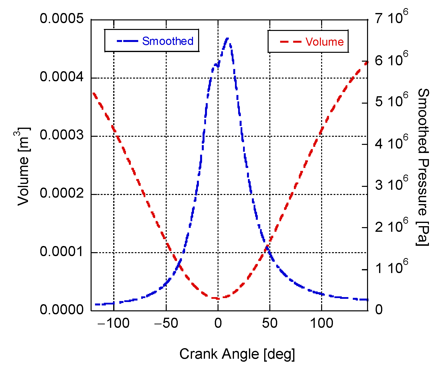
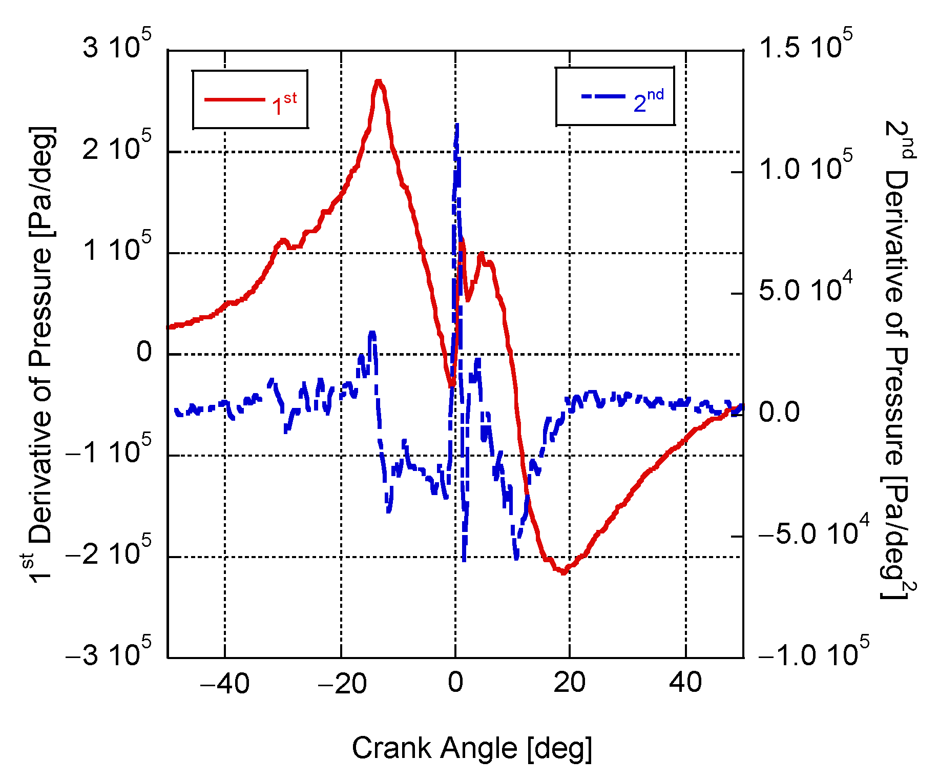
To begin, the model takes in the experimental pressure data and creates a smoothed pressure trace based on a filtering process as shown in Figure 1. This filtering is accomplished by passing the unfiltered pressure trace through a low-pass Chebyshev filter set to 6 kHz, in order to remove high-frequency oscillations and ringing. In addition, the volume and surface area of the cylinder are computed. Using the smoothed pressure data, the first and second derivatives of pressure are computed as illustrated in Figure 2. Syrimis et al. found that the second derivative of pressure can indicate when autoignition happens in the cylinder [43]. Others have postulated that the third derivative of pressure can also provide a quantitative investigation of autoignition [44,45]; however, the use of this option is seen respectively less in the literature. Prior experience in the authors’ laboratory has found that use of the second derivative works well to find ignition timing when employing a single fuel injection event [5]. During multiple fuel injection processes or dual fuel combustion, the use of the second derivative of pressure might not provide a reasonable result, as combustion events might blend. In Figure 2, three representative peaks are seen in the second derivative that correspond to combustion of DME at −31.8° and −14.4° BTDC, with the largest peak occurring at 0.4° ATDC based on the diesel fuel injected at −9.6° BTDC. These peaks presumably correspond to the kinetically limited low-temperature combustion (LTC) followed by a thermal-dissociation dominated high-temperature combustion (HTC) of DME and these phenomena are consistent with the HCCI/PCCI-like DME combustion, as noted by other researchers [46,47]. Thus, visual inspection of the second derivative provides useful insight as to the initiation of multiple phases of combustion in a dual fuel scenario.

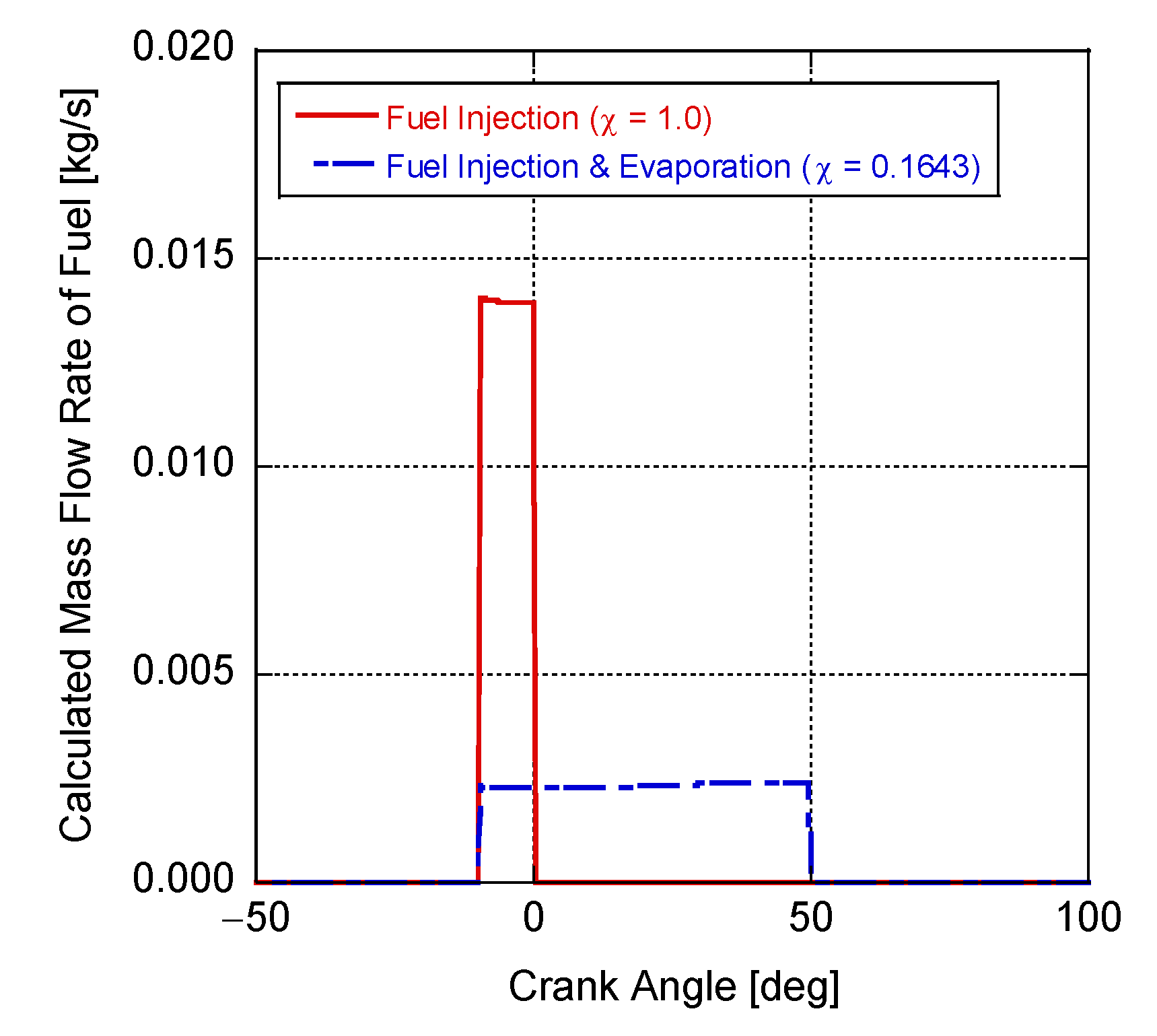
As indicated by Equation (7), the fuel injection profile shown in Figure 3 is computed based on the current pressure difference between the specified nozzle pressure and in-cylinder pressure. However, when it comes to heat release, using this profile as is can create a model artifact, as seen in the early work of the authors [5]. Thus, parameter χ was employed to effectively slow down the fuel injection process to simulate the complete fuel injection, atomization, and evaporation process. An evaporation model, such as that employed by Li et al. [32], that more accurately predicts the evaporation rate of droplets could instead be incorporated. For any direct injected fuel, the relative amount of pre-mixed and diffusion burn combustion will affect this term. With a higher level of diffusion burn, this parameter will likely be lower to account for this respectively slower combustion process. Thus, to obtain a better heat release profile, this parameter was added to an optimization of the heat release rate, which will be discussed later. The result employing this optimized value is provided in Figure 3 and demonstrates a significantly longer overall process. Again, this parameter considers both the fuel injection process and the rate of evaporation of the droplets in the cylinder.

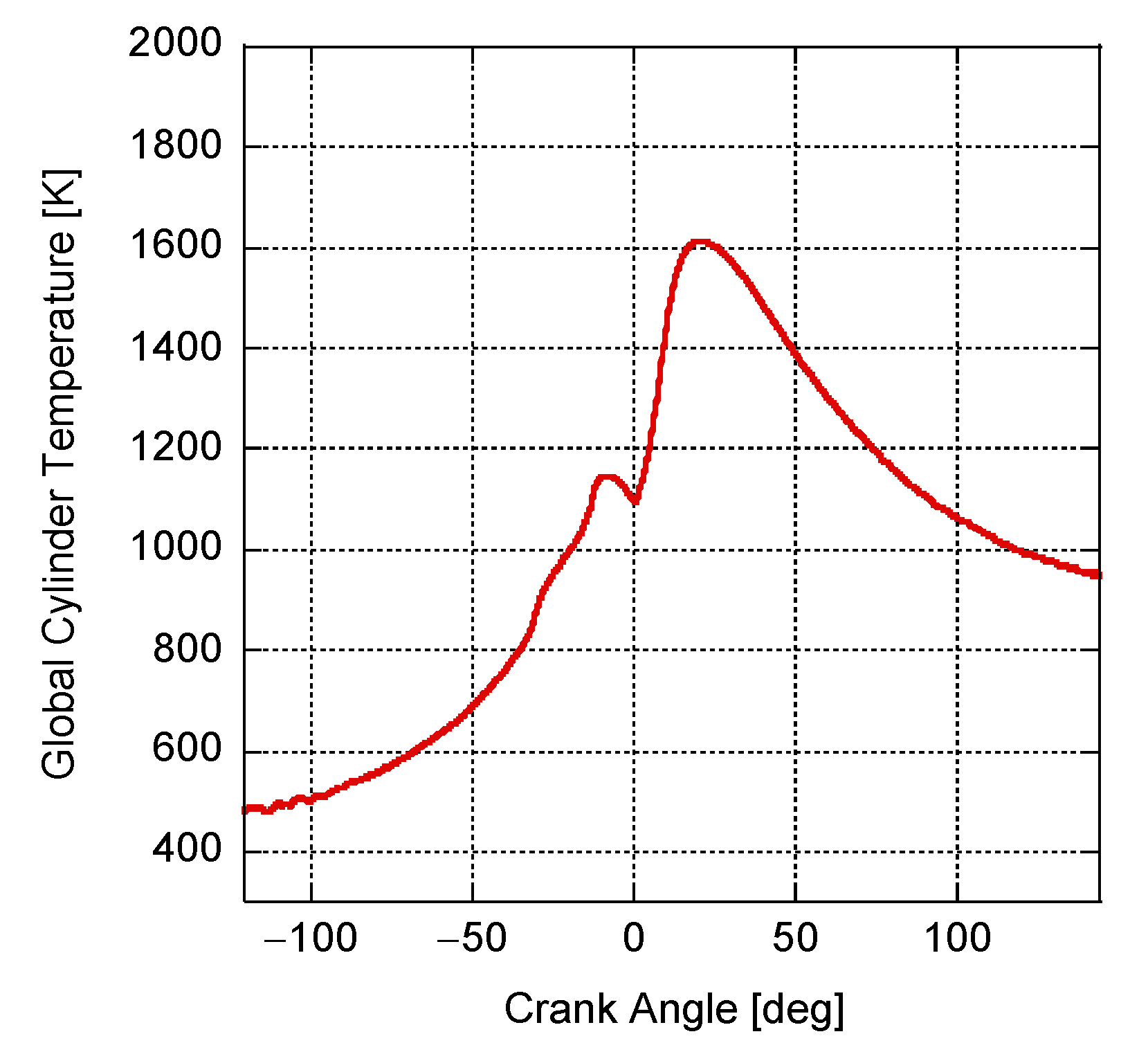
As the model computes the amount of mass in each zone at each step and both the in-cylinder pressure and volume (through geometry) are known, the in-cylinder global temperature can be computed through the ideal gas law as highlighted in Figure 4. It is likely that there are localized spots within the cylinder that will be at higher and lower temperatures; however, a zero-dimensional heat release program cannot capture this fidelity.

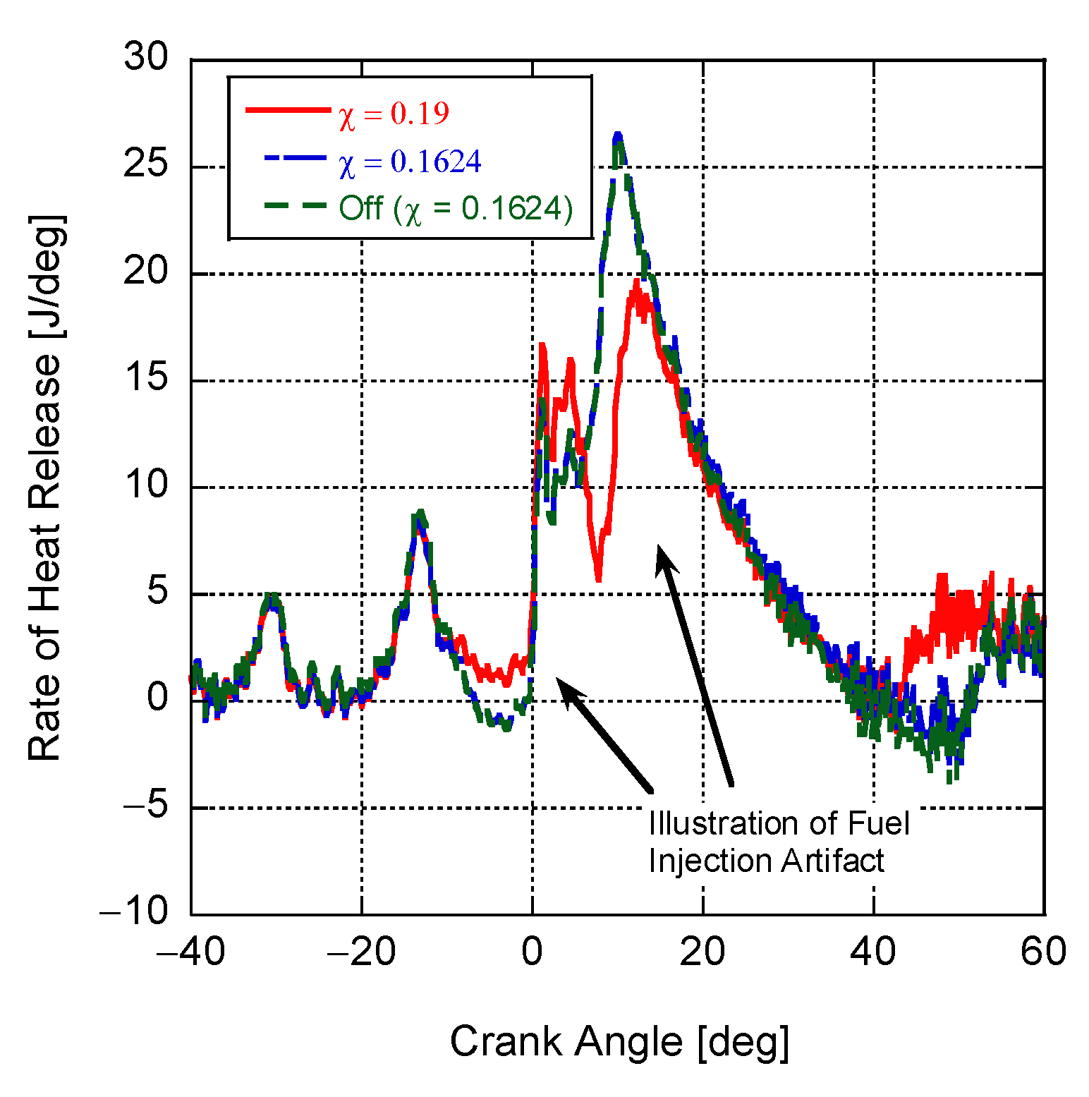
The first law heat release rate on a per degree basis is computed according to Equation (51). In Figure 5, this is provided highlighting (a) the impact of the fuel injection artifact by increasing the value of χ, (b) when the optimized evaporation parameter is utilized, and (c) when the fuel injection terms in the first law are removed from the analysis. Ideally, the model should not demonstrate any fuel injection artifact and (b) and (c) should look similar. For instance, when diesel fuel is injected at −9.6° BTDC, there should be a respective drop in heat release as fuel begins to evaporate, taking energy away from the gas in the cylinder. As illustrated, using a greater value of χ finds that the heat release rate does not decrease as much and prior efforts even demonstrated an incorrect positive heat release rate during fuel injection [5]. Thus, using parameter χ helps adjust the fuel injection and evaporation profile to eliminate this artifact. Overall, the blue curve is the simulated rate of heat release for this experiment.

As DME’s ignition characteristics are temperature-dependent, DME–air mixtures ignite twice, once between 600 and 800 K at lower pressures (~1 atm) and between 800 and 1100 K at higher pressures (~40 bar) [48]. The initial ignition involves competing, low-temperature chemical pathways, whereas the second ignition includes thermal dissociation and the rapid oxidation of the fuel that remains and other intermediate species that were generated during the initial ignition event [49]. Hence, DME-assisted combustion of liquid fuels necessitates careful inspection of the heat release rate.

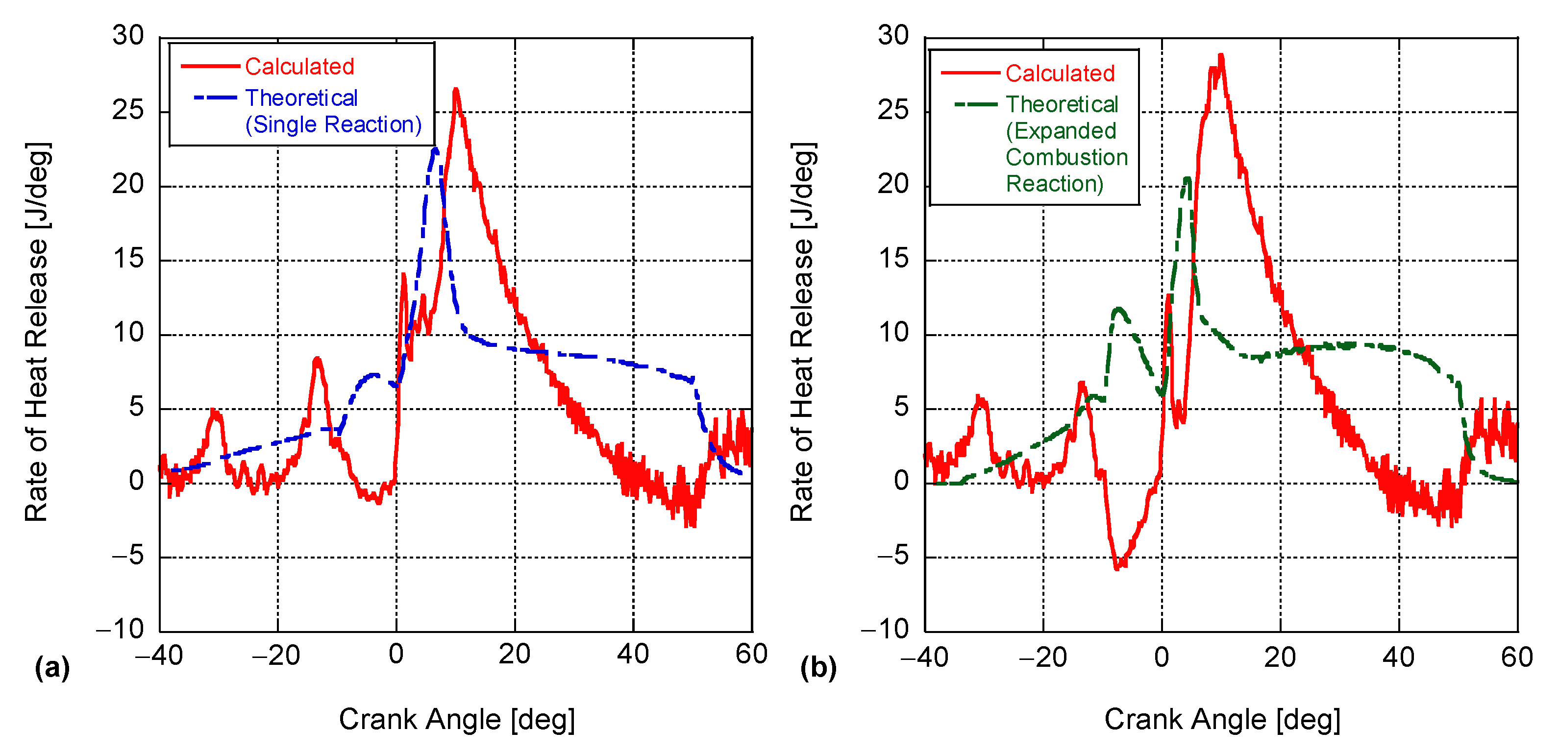
Recall from Equation (67) that a theoretical heat release rate can be determined based on how the chemical species change. Figure 6 highlights the difference between the calculated and theoretical heat release as a function of crank angle. In the first iteration of the model, only a single combustion reaction was used for both fuels (Figure 6a). At that point, it was not expected that the two curves should be the same given the simplified nature of the modeled combustion. A one-step mechanism for both fuels, Equations (17) and (18), was used to simulate the radical pyrolysis of the fuel through the completion of combustion via the carbon monoxide and atomic hydrogen reactions of Equations (32) and (33), respectively. The pre-exponentials, activation energy, and power terms on the mass fractions of oxygen of Equations (17) and (18) along with the evaporation parameter were optimized using the Matlab fmincon function to reduce the difference between the calculated and theoretical heat release rates. Subsequently, combustion was expanded to conclude through the combustion of CO and H₂ while still employing Equations (17) and (18) to simulate radical pyrolysis of Equations (34) and (35). Interestingly, the results after an analogous optimization (Figure 6b) ended up looking like the single localized combustion reaction option. The single combustion reaction provides a more smoothed result over the entire process in comparison with the expanded reaction set. Optimization caused the theoretical results to fall in between the peaks and valleys of DME and ULSD combustion, with the single reaction model having a lower variance, e.g., when ULSD fuel injection happens, the expanded combustion model predicts a greater initial heat release rate. Overall, the model is an improvement on the conventional heat release model of Heywood that effectively employs the ratio of specific heats as a chemical-species-based parameter. However, significant improvements can still be accomplished by adding the radical pyrolysis of the fuel through additional reactions. This will come at a cost of computational complexity and numerical run time. It is envisioned that this will result in an eventual matching of the theoretical and calculated heat release, providing an accurate prediction of the global chemical species in the cylinder. The authors are unaware of any prior heat release model that computes chemical species in this manner.

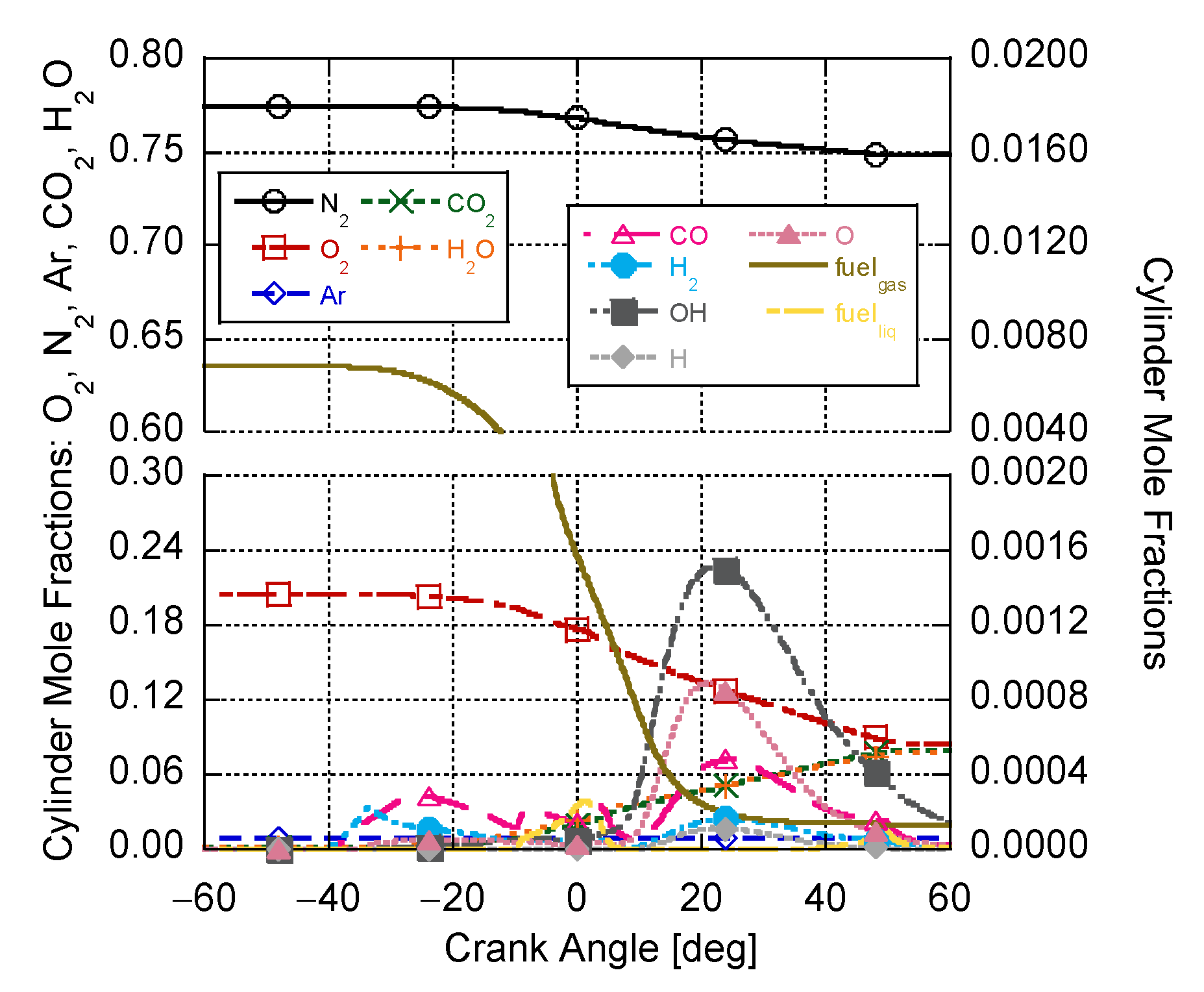
In Figure 7, the global mole fractions of all chemical species including the fuels are provided for the expanded combustion reaction case. The gaseous fuel undergoes a slower combustion process, whereas the direct injected fuel quickly converts to CO and H₂. Again, the optimization process endeavored to match the calculated heat release profile. As a result, a moderate combustion process was predicted for DME to average the heat release between the two peaks seen in the calculated results of Figure 6. For ULSD, the more dramatic rise in heat release (pre-mixed) was captured through the quick conversion of fuel; however, this resulted in an inability to match the later phases of heat release (diffusion burn). The evaporation parameter χ does help with expanding the combustion process to try and capture diffusion burn, but a more complex reaction mechanism is required. Carbon monoxide and hydrogen are indeed being generated from the gaseous and liquid fuels and converted to CO₂ and H₂O, respectively. The creation of hydroxyl chemical species is apparent along with other radical species, highlighting the ability of the model to simulate these components.

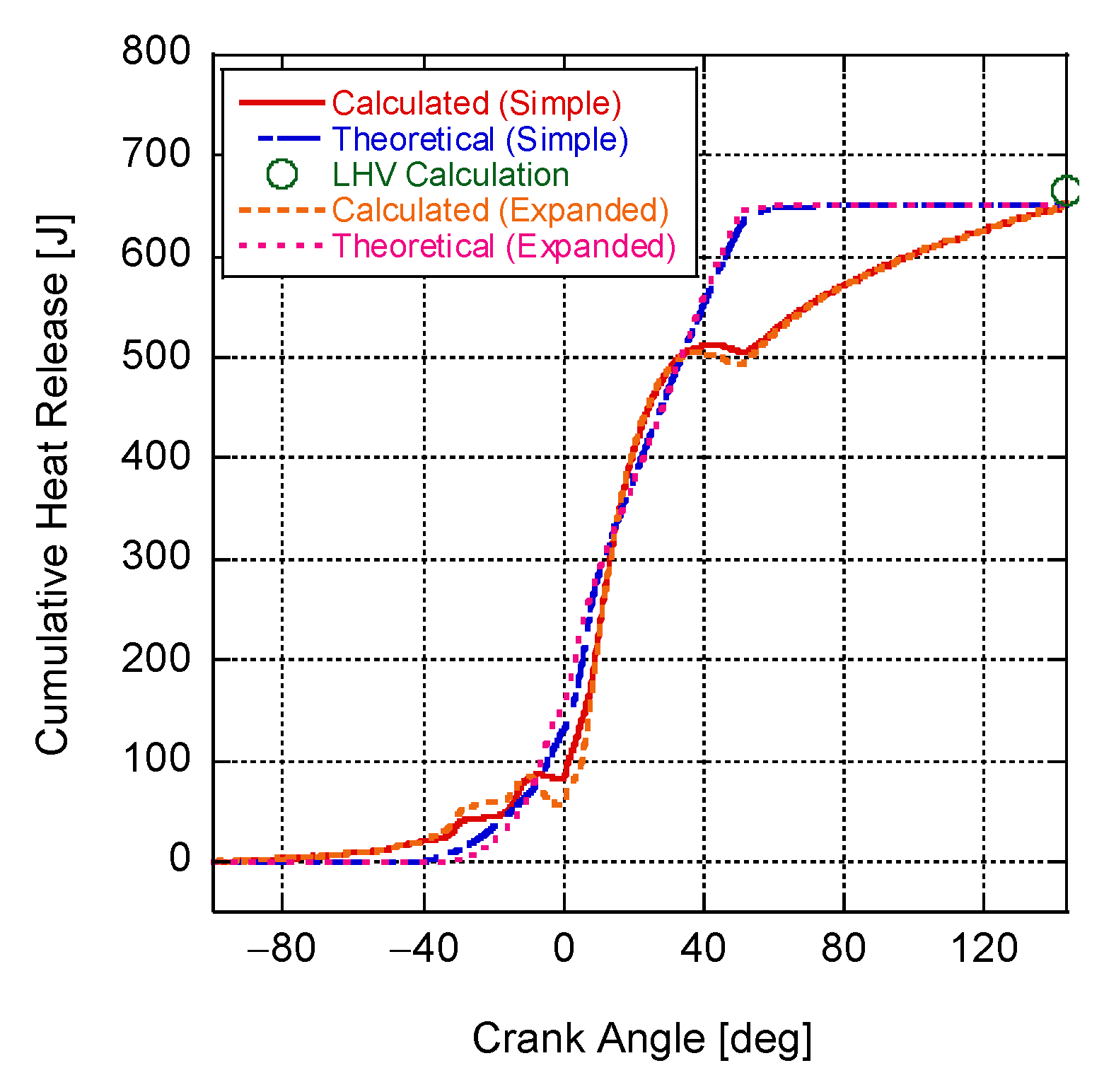
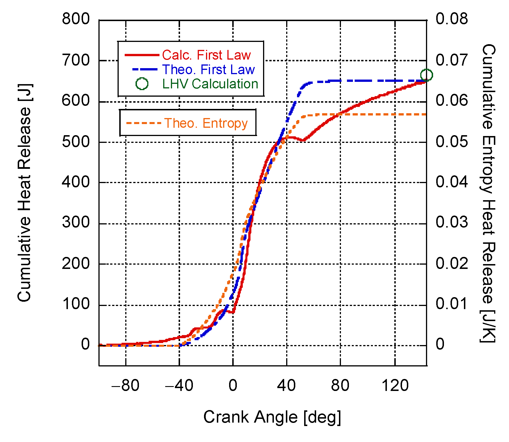
Plotting the cumulative heat te representation of the global chemical species in the crelease based on crank angle in Figure 8 finds that the two combustion models reproduce nearly the same results. The calculated cumulative heat release demonstrates an irregular profile with peaks that correspond to the DME and ULSD crank-angle-based heat release results, whereas the theoretical model predicts a steadier rate of heat release, resulting in a smoother curve. All model results have a lower overall cumulative result than the LHV calculation of Equation (61). This is from the use of CHEMKIN curve-fits and thermodynamic data for all species employed. Again, the discrepancy from the theoretical species results and the calculated heat release model is seen clearly with the later stages of combustion less accurately predicted from a species perspective. Future efforts should target the matching of both Figure 6 and Figure 8 through an enhanced reaction mechanism to provide an accuraylinder.

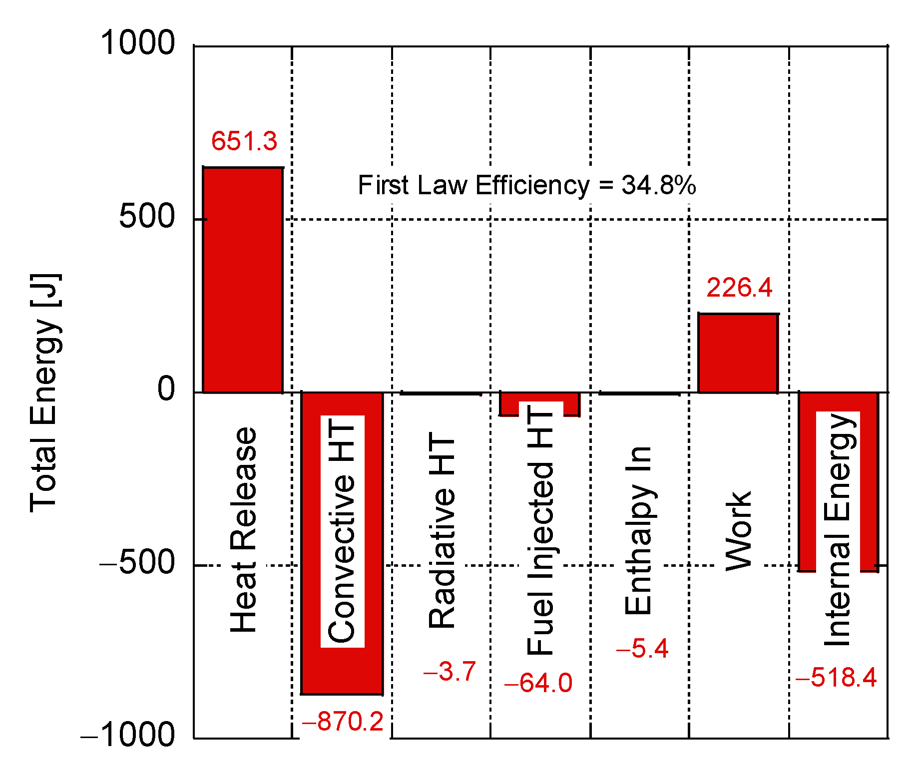
As there was no appreciable difference between the simple and expanded combustion models, only the simple combustion model results are presented moving forward. Figure 9 highlights the different energy components of the conservation of energy equation and a check according to Equation (51) finds that they balance. As to be expected, radiative heat transfer is significantly less than convective heat transfer, which dominates the losses. Interestingly, heat transfer due to fuel injection is a non-insignificant value stemming from the respectively high load simulated for this engine that required a large fuel injection event. From this information, the first law efficiency of the engine can be calculated from the work and cumulative heat release.

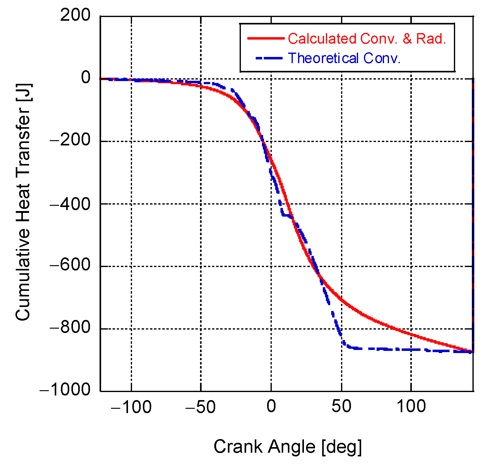
If the theoretical heat release is computed through the species correctly, recalling the discussion around Equation (68) indicates that it would be possible to back calculate the theoretical convective heat transfer rate that balances the first law at each crank angle. This could be used to develop a new heat transfer correlation that is more accurate than current models [40]. Figure 10 highlights the comparison between the calculated convective and radiative heat transfer and the theoretical convective heat transfer from Equation (68). As the calculated convective heat transfer was calibrated to match the cumulative heat release rate at EVO, it is not surprising that the curves are similar. Differences are largely seen towards the latter stages of combustion as the species are inaccurately predicted. However, the respective goodness of fit (R² = 0.992) lends credence to the use of the heat transfer model employed.

Owing to the impact of entropy generation, there is no method to calculate the entropy heat release from the data. In other words, entropy heat release is embedded within the entropy generation term without any method of separating it into two terms, like the first law of thermodynamics. The conservation of entropy equation can be used to determine the relative influence of each expression, as shown in Figure 11. Heat transfer is the largest factor for entropy generation, with the convective and radiative components being significant. Combustion embedded in the control volume entropy has the second largest influence, with the fuel injection process having a small impact. The entropy flowing in has an incorrect negative impact on entropy generation. This is likely due to the choice of the equilibrium vapor pressure when calculating the pressure component in Equation (72); hence, this assumption should be revisited. The Carnot efficiency is calculated from the ambient temperature during the experiment and the maximum global in-cylinder temperature.

While the entropy heat release cannot be calculated through the conservation of entropy equation, it can be determined theoretically through Equation Figure 12 shows the theoretical cumulative entropy heat release plotted along with the first law heat release values of Figure 8. Interestingly, in comparison with Figure 11, the cumulative entropy heat release value due to combustion is respectively small in comparison with the other facets of entropy generation. It only accounts for about 15% of the entropy generated within the control volume and pales in magnitude compared with entropy generated through heat transfer.

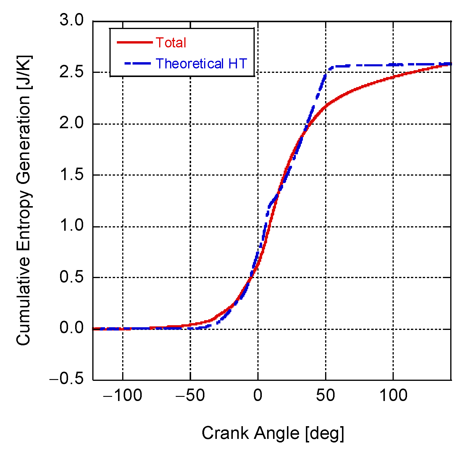
Recalling the discussion around Figure 10 and the determination of a theoretical heat transfer, it is possible to use this expression for finding entropy generation. Figure 13 highlights the entropy generation computed using the conservation of entropy equation and whether the heat transfer in this equation was replaced with the theoretical convective heat transfer determined for Figure 10. Again, they end at the same cumulative result because the total heat release was matched through modifying the convective heat transfer correlation. Like the discussion around Figure 10, it is not surprising that the curves are comparable, with discrepancies seen during the later stages of combustion. However, the respective matching does lend further credibility to the fact that the heat transfer correlation chosen is appropriate. In addition, comparison of these curves provides another potential check on the reaction mechanism employed.

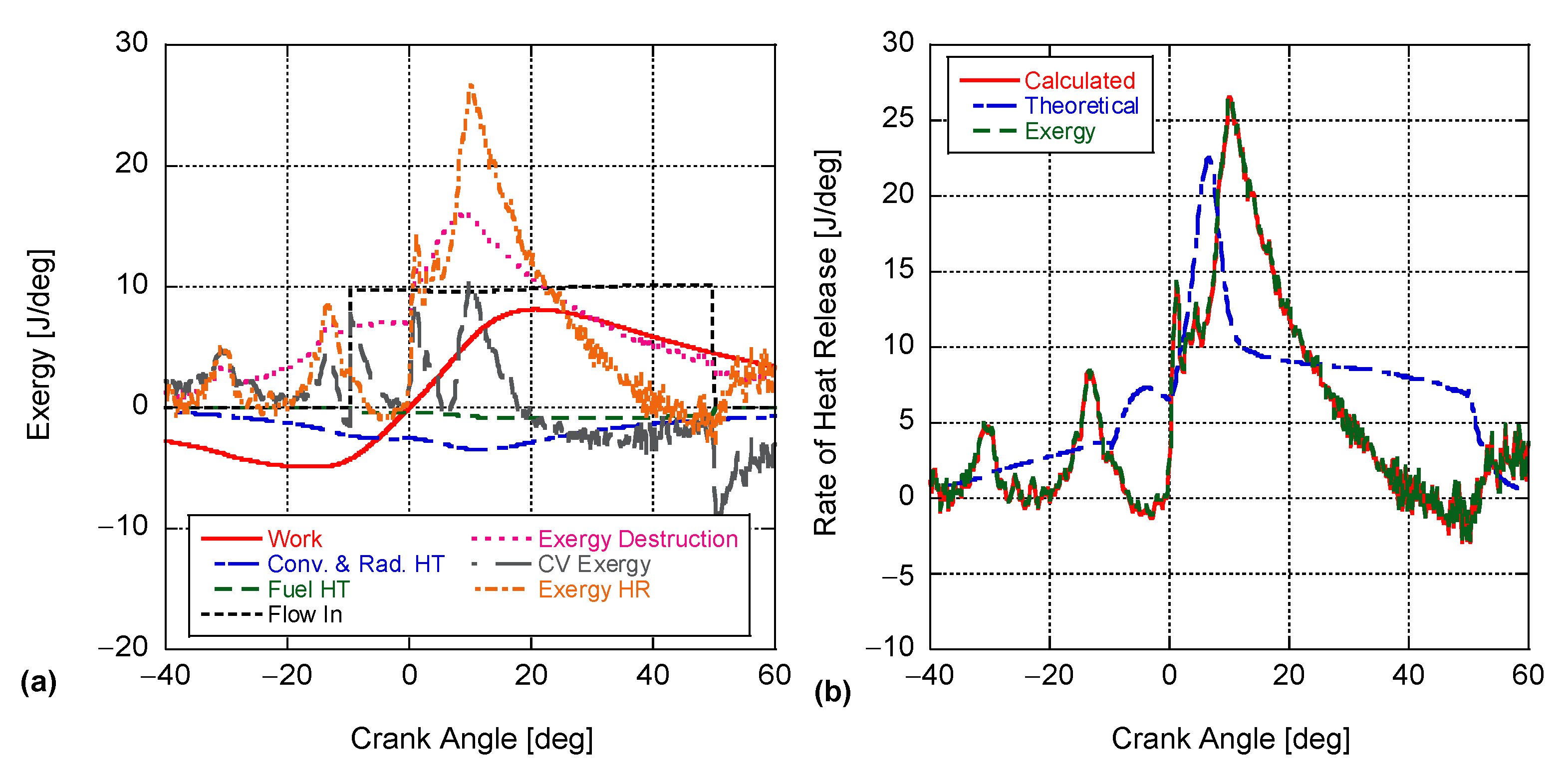
In Figure 14a, the exergy components on a per degree basis are presented. As ULSD has a significant amount of chemical exergy, the fuel injection process (i.e., flow in) demonstrates a relatively steady addition of exergy that corresponds to the profile in Figure 3. Exergy destruction also has a noticeable influence on the level of exergy within the system, whereas heat transfer has a respectively lower impact. The losses and gains in work exergy follow the compression and expansion processes, as expected. Interestingly, the control volume exergy encounters a significant number of positive peaks, highlighting advantageous combustion events of both DME and ULSD. Like the conservation of energy, an exergy heat release can be computed from the data that nearly exactly follows the conservation of energy heat release, as seen in Figure 14b.

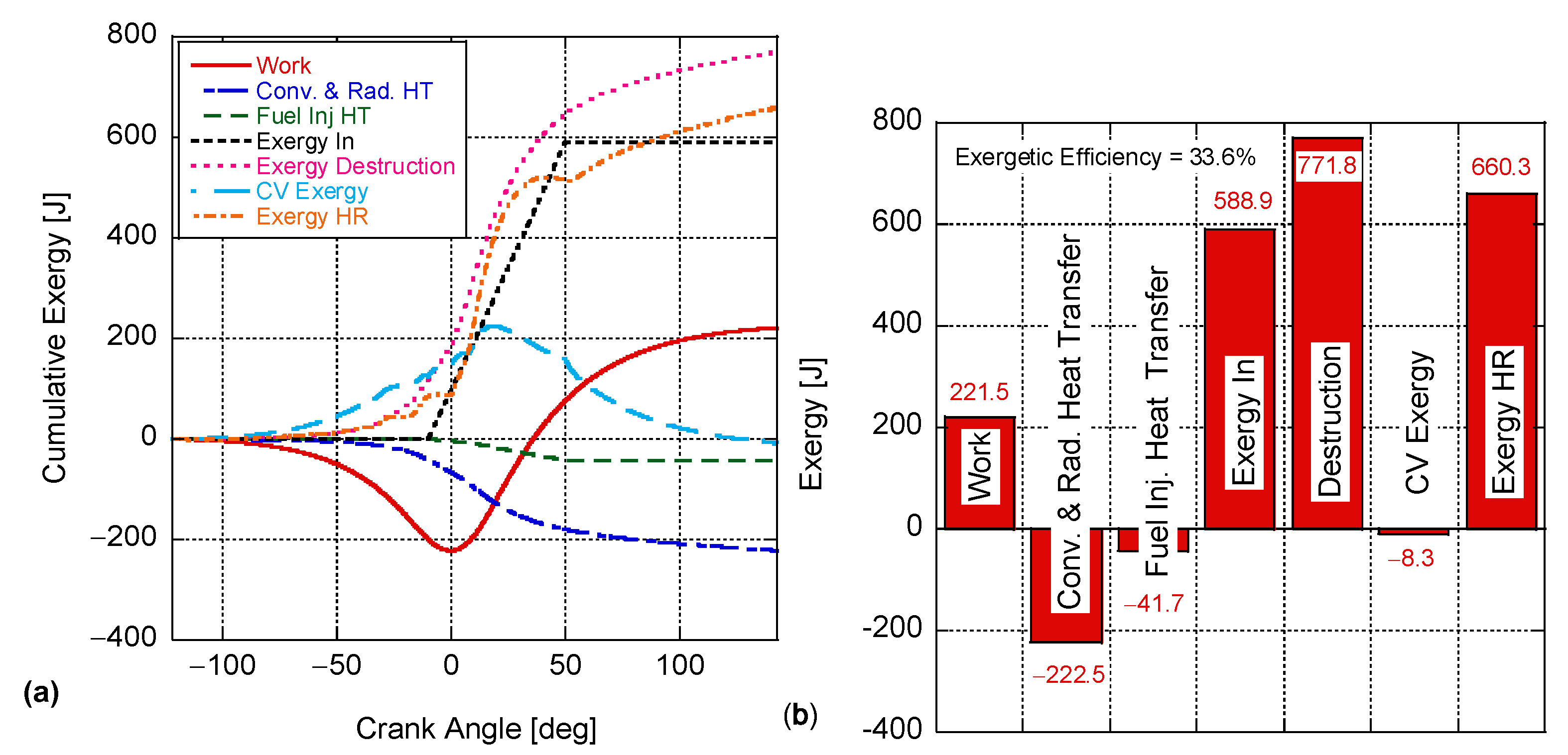
Figure 15a presents the exergy results on a cumulative basis and Figure 15b illustrates the final cumulative impact of the different constituents according to Equation (76). The generation of useful work pulls exergy out of the control volume, while the combined heat transfer loses more exergy overall. The direct fuel injection process adds a significant amount of exergy into the system and most exergy is lost through destruction and irreversibilities. As a result, a lower exergetic efficiency is seen in comparison with the first law efficiency, highlighting the negative aspects of heat transfer and irreversibilities.

Like the conservation of energy and conservation of entropy, a theoretical exergy heat release can be determined through Equation (85). Figure 16 provides the cumulative theoretical heat release values plotted with the calculated values from the energy and exergy equations. The same difference between the theoretical and calculated exergy values as that of energy regarding Figure 8 is seen. As stated before, if the chemical species are simulated correctly, there should be little difference between the calculated and theoretical values. Exergy then provides one last check of correctness between model predictions and values calculated from the experimental data. Finally, this figure demonstrates a minor difference in the cumulative results between energy and exergy that stems from exergy’s reference state calculation.

5. Recommendations

At present, the heat release model has room for expansion in a number of areas. Most prominently is the characterization of engine-out heat transfer, which has long been a source of uncertainty. This heat transfer will vary depending on cylinder and piston geometry, cooling methods, and application. While this will be dependent on the engine and test cell configurations of individual researchers, the model at present may be well-suited to more accurate heat transfer estimations owing to the inclusion of entropy and exergy equations in the core of the model. In addition, a standard set of experimental data for the validation of heat release models would be helpful. Measurements of heat release inside the cylinder through optical or laser-based combustion analysis would help ensure model correctness while expanding the predictive nature of the model through the construction of better sub-models for fuel injection and vaporization. Capturing exhaust emissions at the same time could additionally help the formulation of enhanced chemical kinetics. Furthermore, the combustion model can be expanded significantly to include partial oxidation to CO and H₂, inclusion of additional side reactions (e.g., water gas shift and steam reforming), radical pyrolysis of the fuel, and nitrogen oxide production. Thus, global, reduced, and/or detailed kinetic mechanisms could be included along with an interpreter program, such as Cantera [50]. Finally, validation of the model using different fuels, load points, EGR rates, and so on would be helpful to highlight model shortcomings and additional areas for improvement.

6. Conclusions

Quantifying engine performance metrics through heat release rate analysis is paramount for improving their combustion performance and lowering emissions. Common heat release rate models lack fidelity as they do not track the chemical species change accurately and rarely employ the second law of thermodynamics or exergy. Therefore, this effort proposes an optimized open-source, multi-zone 0D diagnostic heat release rate model to (a) track chemical species progression between IVC and EVO relatively accurately, (b) predict heat release rate from in-cylinder pressure measurements and engine operational characteristics via the first law, and (c) compute entropy generation from the second law along with the exergy balance, for various runtime conditions (e.g., single-fuel, dual-fuel, EGR) using a relatively small set of reaction kinetics. The main features of this model are its open-source framework, the addition of the second law and exergy to provide a correctness check, and modularity (i.e., the model can utilize global and detailed reaction mechanisms to represent fuel combustion). Moreover, the entropy heat release expression (potentially unique in the literature) can be used to compare fuels based on a relative comparison of energy to entropy release.

Model validation against experimental data found that this model accurately estimates ignition timing and the low- and high-temperature combustion of DME-assisted diesel combustion from the second derivative of in-cylinder pressure, thus providing a useful insight into the different phases of combustion in a dual-fuel scenario. The use of a simple dampening coefficient χ to adjust fuel injection and evaporation profile minimizes artifacts, improves the results’ accuracy, and reduces the computational effort. Moreover, the theoretical heat release computation from species shows a high goodness of fit (R² = 0.992) and suggests that the model can be used to develop a new heat transfer correlation for better accuracy. The second law analysis confirms that the impact of physical/chemical processes on entropy generation is in the order of heat transfer > combustion > fuel injection. Furthermore, the entropy and exergy calculations provide a correctness check and successfully capture the advantageous combustion events of DME and ULSD. In addition, the model predicts a lower exergetic efficiency that highlights the negative aspects of heat transfer and irreversibilities.

While the model results appear satisfactory, it has its limitations. Firstly, the use of the second derivative of pressure might not always provide reasonable results under multiple fuel injections or dual fuel combustion. Secondly, the 0D model cannot capture the effect of localized in-cylinder hot and cold spots on fuel combustion and emission formation. Additionally, using a global combustion reaction can lower model fidelity. Overall, this is an improved iteration of the conventional heat release model based on a robust methodology to correctly investigate combustion and emission performance under varying engine operation conditions. It can be further expanded to include any mass exiting the cylinder and blow-by past the cylinder. Finally, detailed fuel pyrolysis and combustion reactions can be added to the model to improve the prediction of in-cylinder global chemical species.

References

- Heywood, J.B. Internal Combustion Engine Fundamentals, 2nd ed.; McGraw-Hill Education: New York, NY, USA, 2018. [Google Scholar]
- Gatowski, J.A.; Balles, E.N.; Chun, K.M.; Nelson, F.E.; Ekchian, J.A.; Heywood, J.B. Heat Release Analysis of Engine Pressure Data. SAE Trans. 1984, 93, 961–977. [Google Scholar] [CrossRef]
- Abbaszadehmosayebi, G.; Ganippa, L. Characterising Wiebe Equation for Heat Release Analysis based on Combustion Burn Factor (Ci). Fuel 2014, 119, 301–307. [Google Scholar] [CrossRef]
- Mattson, J.M.S.; Depcik, C. Emissions-Calibrated Equilibrium Heat Release Model for Direct Injection Compression Ignition Engines. Fuel 2014, 117, 1096–1110. [Google Scholar] [CrossRef]
- Mangus, M.; Kiani, F.; Mattson, J.; Tabakh, D.; Petka, J.; Depcik, C.; Peltier, E.; Stagg-Williams, S. Investigating the Compression Ignition Combustion of Multiple Biodiesel/ULSD (Ultra-Low Sulfur Diesel) Blends via Common-Rail Injection. Energy 2015, 89, 932–945. [Google Scholar] [CrossRef]
- Rakopoulos, D.C. Heat Release Analysis of Combustion in Heavy-Duty Turbocharged Diesel Engine Operating on Blends of Diesel Fuel with Cottonseed or Sunflower Oils and Their Bio-diesel. Fuel 2012, 96, 524–534. [Google Scholar] [CrossRef]
- Egnell, R. The Influence of EGR on Heat Release Rate and NO Formation in a DI Diesel Engine; SAE Technical Paper 2000-01-1807; Society of Automotive Engineering, Inc.: Warrendale, PA, USA, 2000. [Google Scholar] [CrossRef]
- Langness, C.; Mattson, J.; Depcik, C. Moderate Substitution of Varying Compressed Natural Gas Constituents for Assisted Diesel Combustion. Combust. Sci. Technol. 2017, 189, 1354–1372. [Google Scholar] [CrossRef]
- Mattson, J.; Langness, C.; Niles, B.; Depcik, C. Usage of glycerin-derived, hydrogen-rich syngas augmented by soybean biodiesel to power a biodiesel production facility. Int. J. Hydrogen Energy 2016, 41, 17132–17144. [Google Scholar] [CrossRef]
- Mattson, J.M.S.; Langness, C.; Depcik, C. An Analysis of Dual-Fuel Combustion of Diesel with Compressed Natural Gas in a Single-Cylinder Engine; SAE Technical Paper 2018-01-0248; Society of Automotive Engineering, Inc.: Warrendale, PA, USA, 2018. [Google Scholar] [CrossRef]
- Ortiz-Soto, E.A.; Lavoie, G.A.; Martz, J.B.; Wooldridge, M.S.; Assanis, D.N. Enhanced Heat Release Analysis for Advanced Multi-Mode Combustion Engine Experiments. Appl. Energy 2014, 136, 465–479. [Google Scholar] [CrossRef] [Green Version]
- Sitaraman, R.; Batool, S.; Borhan, H.; Velni, J.M.; Naber, J.D.; Shahbakhti, M. Data-Driven Model Learning and Control of RCCI Engines based on Heat Release Rate. IFAC-PapersOnLine 2022, 55, 608–614. [Google Scholar] [CrossRef]
- Catania, A.E.; Misul, D.; Mittica, A.; Spessa, E. A Refined Two-Zone Heat Release Model for Combustion Analysis in SI Engines. JSME Int. J. Ser. B 2003, 46, 75–85. [Google Scholar] [CrossRef] [Green Version]
- Gu, J.; Song, Y.; Wang, Y.; Meng, W.; Shi, L.; Deng, K. Prediction of heat release and NOx emissions for direct-injection diesel engines using an innovative zero-dimensional multi-phase combustion model. Fuel 2022, 329, 125438. [Google Scholar] [CrossRef]
- Li, R.C.; Zhu, G.G.; Men, Y. A two-zone reaction-based combustion model for a spark-ignition engine. Int. J. Engine Res. 2021, 22, 109–124. [Google Scholar] [CrossRef]
- DelVescovo, D.A.; Kokjohn, S.L.; Reitz, R.D. A Methodology for Studying the Relationship Between Heat Release Profile and Fuel Stratification in Advanced Compression Ignition Engines. Front. Mech. Eng. 2020, 6, 28. [Google Scholar] [CrossRef]
- Abbaszadehmosayebi, G.; Ganippa, L. Determination of Specific Heat Ratio and Error Analysis for Engine Heat Release Calculations. Appl. Energy 2014, 122, 143–150. [Google Scholar] [CrossRef]
- Gainey, B.; Longtin, J.P.; Lawler, B. A Guide to Uncertainty Quantification for Experimental Engine Research and Heat Release Analysis. SAE Int. J. Engines 2019, 12, 509–523. [Google Scholar] [CrossRef]
- Oppenheim, A.K.; Barton, J.E.; Kuhl, A.L.; Johnson, W.P. Refinement of Heat Release Analysis; SAE Technical Paper Series; Society of Automotive Engineering, Inc.: Warrendale, PA, USA, 1997. [Google Scholar] [CrossRef]
- Sen, A.K.; Litak, G.; Finney, C.E.A.; Daw, C.S.; Wagner, R.M. Analysis of Heat Release Dynamics in an Internal Combustion Engine Using Multifractals and Wavelets. Appl. Energy 2010, 87, 1736–1743. [Google Scholar] [CrossRef]
- Timoney, D.J. Problems with Heat Release Analysis in D.I. Diesels; SAE Technical Paper 870270; Society of Automotive Engineering, Inc.: Warrendale, PA, USA, 1987. [Google Scholar] [CrossRef]
- Jafarmadar, S. Three-Dimensional Modeling and Exergy Analysis in Combustion Chambers of an Indirect Injection Diesel Engine. Fuel 2013, 107, 439–447. [Google Scholar] [CrossRef]
- Mattson, J.; Reznicek, E.; Depcik, C. Second Law Heat Release Modeling of a Compression Ignition Engine Fueled with Blends of Palm Biodiesel. In Proceedings of the ASME 2015 International Mechanical Engineering Congress and Exposition, Houston, TX, USA, 13–19 November 2015; Volume 6B. [Google Scholar] [CrossRef]
- Ramos da Costa, Y.J.; Barbosa de Lima, A.G.; Bezerra Filho, C.R.; de Araujo Lima, L. Energetic and Exergetic Analyses of a Dual-Fuel Diesel Engine. Renew. Sustain. Energy Rev. 2012, 16, 4651–4660. [Google Scholar] [CrossRef]
- Mattson, J.; Langness, C.; Depcik, C. Exergy Analysis of Dual-Fuel Operation with Diesel and Moderate Amounts of Compressed Natural Gas in a Single-Cylinder Engine. Combust. Sci. Technol. 2017, 190, 471–489. [Google Scholar] [CrossRef]
- Mattson, J.M.S. Modeling of Compression Ignition Engines for Advanced Engine Operation and Alternative Fuels by the Second Law of Thermodynamics. Ph.D. Thesis of Philosophy, Department of Mechanical Engineering, University of Kansas, Lawrence, KS, USA, 2019. [Google Scholar]
- Eaton, J.W. GNU Octave. 2023. Available online: https://octave.org/ (accessed on 4 March 2023).
- Depcik, C. Open-Source Energy, Entropy, and Exergy 0-D Heat Release Model for Internal Combustion Engines. Available online: https://github.com/depcik/heat-release (accessed on 4 March 2023).
- De Renzis, E.; Mariani, V.; Bianchi, G.M.; Cazzoli, G.; Falfari, S.; Antetomaso, C.; Irimescu, A. Implementation of a Multi-Zone Numerical Blow-by Model and Its Integration with CFD Simulations for Estimating Collateral Mass and Heat Fluxes in Optical Engines. Energies 2021, 14, 8566. [Google Scholar] [CrossRef]
- Stiesch, G.; Merker, G.P. A Phenomenological Model for Accurate and Time Efficient Prediction of Heat Release and Exhaust Emissions in Direct-Injection Diesel Engines; SAE Technical Paper 1999-01-1535; Society of Automotive Engineering, Inc.: Warrendale, PA, USA, 1999. [Google Scholar] [CrossRef]
- Assanis, D.; Filipi, Z.; Fiveland, S.B.; Syrimis, M. A Methodology for Cycle-By-Cycle Transient Heat Release Analysis in a Turbocharged Direct-Injection Diesel Engine; SAE Technical Paper 2000-01-1185; Society of Automotive Engineering, Inc.: Warrendale, PA, USA, 2000. [Google Scholar] [CrossRef]
- Li, J.; Yang, S.; Yang, J.; Rao, S.; Zeng, Q.; Li, F.; Chen, Y.; Xia, Q.; Li, K. Heat transfer for a single deformed evaporating droplet in the internal combustion engine. Phys. Lett. A 2021, 411, 127555. [Google Scholar] [CrossRef]
- Nishida, K.; Hiroyasu, H. Simplified Three-Dimensional Modeling of Mixture Formation and Combustion in a D.I. Diesel Engine; SAE Technical Paper 890269; Society of Automotive Engineering, Inc.: Warrendale, PA, USA, 1989. [Google Scholar] [CrossRef]
- Alam, S.S.; Depcik, C. Verification and Validation of a Homogeneous Reaction Kinetics Model Using a Detailed H2-O2 Reaction Mechanism Versus Chemkin and Cantera. In Proceedings of the ASME 2019 International Mechanical Engineering Congress and Exposition, Salt Lake City, UT, USA, 11–14 November 2019. [Google Scholar] [CrossRef]
- Smith, G.P.; Golden, D.M.; Frenklach, M.; Moriarty, N.W.; Eiteneer, B.; Goldenberg, M.; Bowman, C.T.; Hanson, R.K.; Song, S.; William, C.; et al. GRI-MECH 3.0. Available online: http://combustion.berkeley.edu/gri-mech/version30/text30.html (accessed on 30 January 2022).
- Burke, M.P.; Chaos, M.; Ju, Y.; Dryer, F.L.; Klippenstein, S.J. Comprehensive H2/O2 kinetic model for high-pressure combustion. Int. J. Chem. Kinet. 2012, 44, 444–474. [Google Scholar] [CrossRef]
- Li, J.; Zhao, Z.; Kazakov, A.; Chaos, M.; Dryer, F.L.; Scire, J.J., Jr. A comprehensive kinetic mechanism for CO, CH2O, and CH3OH combustion. Int. J. Chem. Kinet. 2007, 39, 109–136. [Google Scholar] [CrossRef]
- Woschni, G. Universally Applicable Equation for the Instantaneous Heat Transfer Coefficient in the Internal Combustion Engine; SAE Paper 670931; Society of Automotive Engineering, Inc.: Warrendale, PA, USA, 1967. [Google Scholar] [CrossRef]
- Hohenberg, G.F. Advanced Approaches for Heat Transfer Calculations; SAE Paper 790825; Society of Automotive Engineering, Inc.: Warrendale, PA, USA, 1979. [Google Scholar] [CrossRef]
- Depcik, C.; Alam, S.S.; Madani, S.; Ahlgren, N.; McDaniel, E.; Burugupally, S.P.; Hobeck, J. Determination of a Heat Transfer Correlation for Small Internal Combustion Engines. Submitt. Appl. Therm. Eng. 2023. [Google Scholar]
- Kee, R.J.; Rupley, F.M.; Meeks, E.; Miller, J.A. Chemkin-III: A Fortran Chemical Kinetics Package for the Analysis of Gas-Phase Chemical and Plasma Kinetics; SAND96-8216; Sandia National Laboratories: Albuquerque, NM, USA, 1996. [Google Scholar]
- Langness, C.; Mangus, M.; Depcik, C. Construction, Instrumentation, and Implementation of a Low Cost, Single-Cylinder Compression Ignition Engine Test Cell; SAE Technical Paper 2014-01-0673; Society of Automotive Engineering, Inc.: Warrendale, PA, USA, 2014. [Google Scholar] [CrossRef]
- Syrimis, M.; Shigahara, K.; Assanis, D.N. Correlation Between Knock Intensity and Heat Transfer Under Light and Heavy Knocking Conditions in a Spark Ignition Engine. SAE Trans. 1996, 105, 592–605. [Google Scholar] [CrossRef]
- Puzinauskas, P.V. Examination of Methods Used to Characterize Engine Knock; SAE Technical Paper 920808; Society of Automotive Engineering, Inc.: Warrendale, PA, USA, 1992. [Google Scholar] [CrossRef]
- Checkel, M.D.; Dale, J.D. Testing a Third Derivative Knock Indicator on a Production Engine; SAE Technical Paper; Society of Automotive Engineering, Inc.: Warrendale, PA, USA, 1986. [Google Scholar] [CrossRef]
- Theinnoi, K.; Suksompong, P.; Temwutthikun, W. Engine Performance of Dual Fuel Operation with In-cylinder Injected Diesel Fuels and In-Port Injected DME. Energy Procedia 2017, 142, 461–467. [Google Scholar] [CrossRef]
- Wang, Y.; Zhao, Y.; Xiao, F.; Li, D. Combustion and emission characteristics of a diesel engine with DME as port premixing fuel under different injection timing. Energy Convers. Manag. 2014, 77, 52–60. [Google Scholar] [CrossRef]
- Deng, S.; Zhao, P.; Zhu, D.; Law, C.K. NTC-affected ignition and low-temperature flames in nonpremixed DME/air counterflow. Combust. Flame 2014, 161, 1993–1997. [Google Scholar] [CrossRef]
- Krisman, A.; Hawkes, E.R.; Talei, M.; Bhagatwala, A.; Chen, J.H. Polybrachial structures in dimethyl ether edge-flames at negative temperature coefficient conditions. Proc. Combust. Inst. 2015, 35, 999–1006. [Google Scholar] [CrossRef]
- Goodwin, D.G.; Speth, R.L.; Moffat, H.K.; Weber, B.W. Cantera: An Object-Oriented Software Toolkit for Chemical Kinetics, Thermodynamics, and Transport Processes. 2023. Available online: https://www.cantera.org (accessed on 1 March 2023).
Figure 1.
Smoothed pressure data and the cylinder volume as a function of crank angle.
Figure 2.
The first and second derivatives of pressure based on the filtered pressure as a function of crank angle.
Figure 3.
Calculated mass flow rate of fuel injection as is and including a factor that simply estimates the evaporation process.
Figure 4.
The global in-cylinder temperature computed from the ideal gas law.
Figure 5.
Rate of heat release on a per degree basis highlighting the injection artifact as a function of the evaporation parameter. The figure also illustrates what the rate of heat release looks like when the corresponding fuel injection terms are removed from the calculation. Single localized combustion reaction.
Figure 6.
The calculated rate of heat release according to the conservation of energy and the theoretical heat release based on the change in chemical species of Equation (67). (a) Single combustion reaction of Section 2.2 and (b) expanded combustion reaction after optimization.
Figure 7.
Global mole fractions of the chemical species in the cylinder as a function of crank angle for the expanded combustion reaction.
Figure 8.
Cumulative heat release calculated based on the first law, from theory, and the final value according to the lower heating values. The figure provides the results from the singular localized combustion reactions (simple) and the expanded combustion reactions (expanded).
Figure 9.
The cumulative energy components of the conservation of energy equation.
Figure 10.
Comparison between the calculated convective and radiative cumulative heat transfer and the theoretical convective only heat transfer that would result using the heat release calculated through the change in chemical species.
Figure 11.
(a) Cumulative entropy generation as a function of crank angle and (b) the results of the different components in the conservation of entropy equation.
Figure 12.
Cumulative heat release calculated based on the first law, from theory, and the final value according to the lower heating values with the theoretical entropy heat release plotted on the second y-axis.
Figure 13.
Cumulative entropy generation computed using the conservation of entropy equation and using a theoretical heat transfer based on the theoretical heat release.
Figure 14.
(a) Exergy components as a function of crank angle and the (b) rate of heat release for the first law and exergy equations.
Figure 15.
(a) Cumulative exergy as a function of crank angle and (b) the results of the different components in the exergy equation.
Figure 16.
Cumulative theoretical conservation of energy, conservation of entropy, and exergy heat release and the calculated conservation of energy and exergy heat release results.
Disclaimer/Publisher’s Note: The statements, opinions and data contained in all publications are solely those of the individual author(s) and contributor(s) and not of MDPI and/or the editor(s). MDPI and/or the editor(s) disclaim responsibility for any injury to people or property resulting from any ideas, methods, instructions or products referred to in the content. |
© 2023 by the authors. Licensee MDPI, Basel, Switzerland. This article is an open access article distributed under the terms and conditions of the Creative Commons Attribution (CC BY) license (https://creativecommons.org/licenses/by/4.0/).
Share and Cite
MDPI and ACS Style
Depcik, C.; Mattson, J.; Alam, S.S. Open-Source Energy, Entropy, and Exergy 0D Heat Release Model for Internal Combustion Engines. Energies 2023, 16, 2514. https://doi.org/10.3390/en16062514
AMA Style
Depcik C, Mattson J, Alam SS. Open-Source Energy, Entropy, and Exergy 0D Heat Release Model for Internal Combustion Engines. Energies. 2023; 16(6):2514. https://doi.org/10.3390/en16062514
Chicago/Turabian StyleDepcik, Christopher, Jonathan Mattson, and Shah Saud Alam. 2023. "Open-Source Energy, Entropy, and Exergy 0D Heat Release Model for Internal Combustion Engines" Energies 16, no. 6: 2514. https://doi.org/10.3390/en16062514
Note that from the first issue of 2016, this journal uses article numbers instead of page numbers. See further details here.