Method Selection for Analyzing the Mesopore Structure of Shale—Using a Combination of Multifractal Theory and Low-Pressure Gas Adsorption

Abstract

Nitrogen adsorption experiments have been extensively applied to shale pore structure research and evaluation. The pore structure can be quantitatively characterized in accordance with the nitrogen adsorption–desorption isotherm using various calculation models, whereas the results obtained using different models can more effectively indicate the pore characteristics of shale remains unclear. Further, there has not been any unified process in the optimization of calculation models for pore size distribution (PSD). In this study, the Barret–Joyner–Halenda adsorption (BJH-AD) and BJH desorption (BJH-DE) models were used with Longmaxi Formation shale as an example. Subsequently, the density functional theory (DFT) calculations were conducted on different shale lithofacies samples. Next, the pore structure parameters and heterogeneity obtained using different models were compared, and the consistency parameters of different models were obtained in accordance with Cronbach’s alpha. The results indicated that the pore structure parameters obtained using the BJH-AD model were underestimated since the macroscopic thermodynamic theory was not applicable to this study. The DFT model showed multiple peaks in the range of 1–10 nm, whereas the BJH-DE model had a significant artificial peak in the range of 3.8 nm due to the tensile strength effect, thus suggesting that the DFT model is more capable of characterizing the pores with a pore size 10 nm lower than the BJH model. The PSD curves generated using the three models exhibited multifractal characteristics, whereas the results of the heterogeneity achieved using different models were different. Moreover, the consistency of the results of different models can be studied in depth by combining Cronbach’s alpha with various heterogeneity parameters. The DFT model exhibited high consistency in pore structure parameters and pore heterogeneity, thus suggesting that the DFT method of N₂ is the optimal physical adsorption data analysis method in the shale mesoporous range. Accordingly, the nitrogen adsorption curve, the hysteresis loop shape, multifractal parameters, and Cronbach’s alpha were integrated to generate a working flow chart of the nitrogen adsorption model for N₂-adsorption-model optimization.

1. Introduction

Since the development and production of shale gas in the Barnett shale block in Texas, shale gas has attracted significant attention worldwide [1,2,3,4]. Through more than 20 years of development, key drilling technologies such as drilling geological guidance and efficient three-dimensional development have been gradually developed from conventional drilling techniques [3,4,5,6]. As an unconventional energy source, the commercial production of shale gas has changed the world’s natural gas trade pattern and has an important place in the energy structure [3,4,5,6,7]. On the one hand, shale is a potential reservoir space for hydrocarbons; on the other hand, it is a potential target for CO₂ sequestration, which can effectively relieve atmospheric CO₂ concentrations [7,8,9,10,11,12,13,14].

In the context of shale gas development, the United States primarily exploits shale gas deposits at burial depths between 1000 and 2000 m in tectonically simple areas, where a significant cumulative thickness and a relatively concentrated layer system have formed. The geological conditions of the Appalachian Basin in the eastern United States are relatively straightforward, with depths rarely exceeding 3000 m, which makes shale gas development less challenging. However, shale gas production formations in China are characterized by rapid changes in sedimentary phases, petrography, and complex sedimentary tectonics, and the quality of different types of shale varies considerably [5,7]. The Wufeng–Longmaxi Formation, for example, is relatively deep, mostly within the range of 2500–4000 m, and that coupled with the complex topography and high formation pressure and temperature makes exploration and development more challenging [3,4,5,7].

Shale pore structure characterization is significant for shale reservoir evaluation and development [9,11,13,15,16,17,18,19,20,21]. However, shale reservoirs are unlike conventional oil and gas reservoirs because of their heterogeneity, low permeability, diverse pore forms, complex pore networks, and extensive and complex pore size distribution (PSD) characterization. The International Union of Pure and Applied Chemistry (IUPAC) classifies the aperture diameter into macropores (>50 nm), mesopores (2–50 nm), and micropores (<2 nm), which is widely used [11,15,16,20,21]. There are several experimental methods to characterize the pore structure of shale reservoirs. Microscopic image analysis, including scanning electron microscopy (SEM) and atomic force microscopy (AFM), can identify pores larger than 5 nm, but its resolution and observation range are limited [1,6,15,21,22,23]; invasive methods include high-pressure mercury injection pore (HPMI) and gas (CO₂ and N₂) adsorption experiments, in which high-pressure mercury injection experiments are prone to damage the samples [11,15,17]. Non-invasive methods, such as nuclear magnetic resonance (NMR), small-angle and ultra-small-angle neutron scattering (SANS/USANS), and computed tomography (CT), are also used [24,25,26]. CT scanning is complex and expensive, and the SANS method has poor measurement results for large-scale rock samples. The NMR method cannot effectively characterize nanoscale pore structure characteristics, which are also affected by paramagnetic compounds [20,25,26].

The field of physical adsorption of porous materials has advanced significantly since 1985, owing to the development of nanoporous materials, high-resolution adsorption experiments that use various subcritical fluids, and the application of various microstructural computational models [27,28,29,30]. Among various experimental methods for shale reservoirs, gas adsorption has been widely applied for surface analysis and structural characterization of nanoporous materials, capable of characterizing porous media materials of less than 200 nm. The presence of a large number of nanoscale pores in shale makes gas adsorption a suitable method for characterizing shale reservoirs [7,14,31]. Due to the difference in gas-saturated vapor pressure, the nitrogen adsorption method is more appropriate for mesopore size distribution analysis, while the CO₂ adsorption method has advantages in measuring micropore size distribution [8,17,29,30,32]. Gas adsorption is not only a non-destructive and relatively convenient method for shale pore structure analysis but also provides a series of information such as pore volume, pore surface area, and PSD under different pore diameters, which effectively reflect the heterogeneity characteristics of shale samples [15,29,30,33,34,35,36,37,38,39,40,41]. Different inversion models are used to obtain relevant pore structure data based on the measured gas adsorption isotherm data. Various theoretical models are employed to calculate pore structure parameters using gas adsorption experiments, including Barrett–Joyner–Halenda (BJH), density functional theory (DFT), Monte Carlo simulation method (MC), Brunauer–Emmett–Teller (BET), Dubinin–Astakhow (DA), Horvath–Kawazoe (HK), and others [42,43,44,45,46,47,48]. The BJH and DFT models are commonly employed to characterize the pore structure of shale, as evidenced by numerous studies [31,32,38]. Previous studies have typically utilized one of the aforementioned methods to analyze shale pore structure [13,15,16,17,18,19,20,21,41]. However, there is no uniform model-selection standard for processing experimental data on shale gas adsorption, which leads to incomparability between different research data. More importantly, it is not clear that the results calculated by different models can better reflect shale pore characteristics. Using the deviation model to describe pore structure can lead to the underestimation or overestimation of reserves, or enhanced oil recovery (EOR) failure, with further economic losses [37].

Many recent works have been conducted on selecting the nitrogen adsorption model. Ravikovitch et al. [45] found that the CO₂ adsorption DFT model was consistent with the MC method in the 0.3–1.5 nm diameters, suggesting the use of the CO₂ adsorption DFT and MC model to study micropore characteristics. Thommes et al. [29] systematically summarized the development history of physical adsorption. Many researchers have compared different methods for characterizing the pore structure of shale reservoirs. For instance, Wang et al. [29] determined that a combination of CO₂ (273 K) adsorption and argon/nitrogen adsorption, respectively, was the standard method for characterizing micro-nanopores. Li et al. [35] compared the pore size distribution (PSD) obtained by the DFT model and the BJH model from the adsorption and desorption curves and found that the PSD curves produced by the BJH model and the DFT model were roughly the same. Similarly, Wei et al. [31] compared different gas adsorption models of shale in the Wufeng–Longmaxi Formation and concluded that the non-local density functional theory (NLDFT) method of N₂ and CO₂ was the most suitable method for analyzing shale gas physical adsorption data. This method has the most appropriate detection range (0.33–100 nm) and has high reliability and accuracy across the entire aperture range. Hazra et al. [49] compared experimental methods for measuring surface area and pore size distributions, including the BET, BJH, and DFT methods. Chandra et al. [50] conducted a systematic analysis of Barakar shale and concluded that the grand canonical Monte Carlo (GCMC) model had a better fit than the DFT model in CO₂ adsorption curves calculating PSD. The former may be the preferred method for estimating the PSD of shale micropores. Additionally, He et al. [40] used the corrected BJH algorithm to calculate the pore size corresponding to the initial point of capillary evaporation of the desorption curve and compared the calculated and measured pore diameters. The error range of the results was within 5%, which verifies the accuracy of the improved BJH algorithm. Pang et al. [32] showed that the Monte Carlo (MC) model had a broader response range and fewer fitting errors than the DFT model, indicating that the MC model was superior to the DFT model in characterizing the microporous structure using CO₂ adsorption data.

The fractal theory has found wide application in the characterization of porous media, including the analysis of pore structure heterogeneity [15,16,20], electrical conductivity [51], and permeability [52]. In the realm of shale reservoirs, the fractal theory represents a powerful tool for pore structure analysis. Researchers have successfully combined the fractal theory with scanning electron microscopy (SEM), low-pressure gas adsorption, micro-CT, high-pressure mercury injection (HPMI), and small-angle neutron scattering (SANS), and have demonstrated that the fractal dimension is a useful parameter for characterizing pore structure [13,15,16,19,20,25,53]. However, due to the pores in shale reservoirs not being uniformly distributed, a single fractal dimension is insufficient for comprehensively characterizing the entirety of the pore structure.

Multifractal theory, as an extension of fractal dimension, enables the acquisition of both global properties and local information by analyzing the probability density fluctuations. This approach has been demonstrated to yield more precise pore structure information in numerous studies [16,26,53,54,55,56,57]. Furthermore, multifractal analysis can describe random fluctuations of aperture in specific intervals and characterize aperture distribution showing various types of self-similarity [54,57,58]. Previous scholars have carried out PSD and NMR T_2C value analysis using multifractal theory [26,55], but few comparative studies have been carried out on different nitrogen adsorption models. Using multifractal theory to optimize different nitrogen adsorption models is the fundamental problem in revealing shale PSD characterization.

In this study, ten shale samples of the Longmaxi Formation in the Sichuan Basin are selected. Nitrogen adsorption experiments, mineral composition, and geochemical parameters of shale samples are carried out. BJH-AD, BJH-DE, and DFT models are used to calculate pore structure parameters such as PV, SA, and PSD. The multifractal dimension parameters are calculated for different PSD models. A series of multifractal parameters are used to test the consistency, and the applicability of different pore structure calculation models is compared and analyzed. Finally, a set of model-selection optimization methods for shale pore size characterization is proposed.

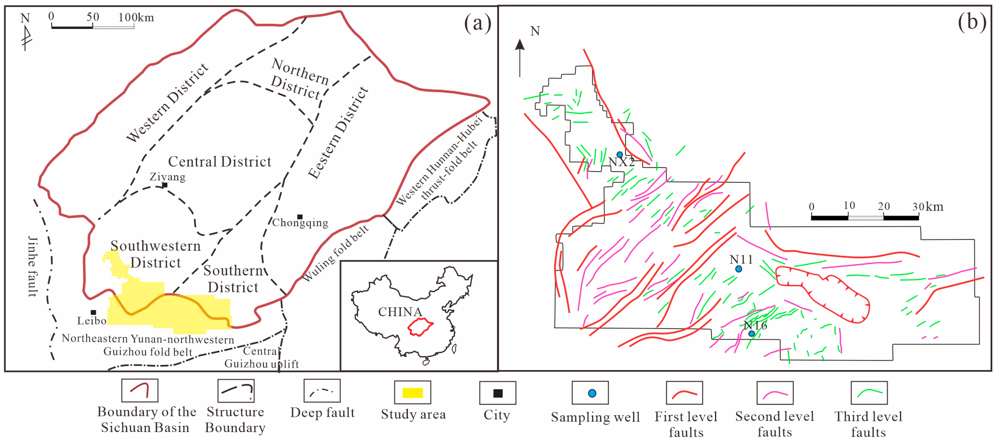
2. Geological Description of the Field

The Sichuan Basin is located in the western Yangtze metaplatform, surrounded by folds and faults, and shows a rhomboid shape covering an area of about 18 × 10⁴ km² [59,60] (Figure 1a). As the primary petroliferous and hydrocarbon-bearing basin, the basin is the most substantial reserve of shale gas resources in China and has experienced large-scale exploration forming the development of conventional and unconventional natural gas reserves. Its tectonic movement and sedimentary evolution includes five stages: Caledonian, Hercynian, Indosinian, Yanshanian, and Himalayan [13,60,61]. Before the late Cretaceous, the south of the Sichuan Basin was dominantly characterized by subsidence and minor uplift. Processing the Yanshanian and Himalayan movements, the Jurassic–Early Cretaceous formation has been eroded with extrusion deformation and assize depth uplift [13,61]. The northwest and southwestern gentle structure zones uplifted during the Caledonian orogeny compresses. A series of sea-level changes, mass extinctions, and glaciations occurred in the Upper Ordovician–Lower Silurian [62], which led to a low-energy, anoxic sedimentary environment [61]. The Wufeng–Longmaxi shale was deposited and preserved with an amount of OM on the deep-water shelf of the Yangtze block [59,60,61] and developed the most critical shale gas exploration and exploitation target stratum, which is characterized by abundant organic matter, high-over thermal maturity, and large thickness, showing the shale gas potential [19,26,59,61].

The Changning gas field is located south of the Sichuan Basin, including the Jianwu low-dipping gentle syncline and exposed Triassic–Silurian strata, which is the dominant commercial shale gas production region in the Sichuan Basin (Figure 1b). Affected by water level changes periodically, the Longmaxi shale displays the variable sedimentary microfacies characteristic, which is composed of dark grey-black siliceous and calcareous shale to the grey-green argillaceous shale of the Longmaxi Formation [59,60]. The thickness of the Longmaxi Formation in the southern Sichuan Basin is stable at approximately 400~600 m, and the current buried depth ranges from 2300 to 3000 m after exhumation. Furthermore, the paleoenvironment changes from the bottom, reducing condition to top segment oxidizing condition, which leads to the different characteristics of hydrocarbon generation potential and gas content [60].

3. Samples and Experimental Methods

In this investigation, we conducted a mineralogical and organic matter geochemical analysis of the shales from the Wufeng–Longmaxi Formation located in southern Sichuan. The purpose was to elucidate the characteristics of the shale matrix composition. We utilized nitrogen adsorption experiments to generate pore size distribution curves using three different adsorption models (BJH-AD, BJH-DE, and DFT). Subsequently, we employed a combination of the multiple fractal theory and nitrogen experiments to compute and derive the inhomogeneity parameters of the shale pore structure. To evaluate the accuracy of the various adsorption models, we utilized the Cronbach coefficient to assess the consistency of the multidimensional inhomogeneity parameters.

3.1. Sample Location and Collection Criterion

In this study, a total of 10 samples were obtained from the lower part of Lower Silurian Longmaxi Formation typical wells from Changning area shale and studied XRD and TOC to identify their mineral composition and geochemical characteristics. The sample selection criterion depends on various TOC and mineral compositions to ensure all lithofacies categories have corresponding samples. Sampling burial depths are 2490.5~4355.4 m, and the sampling well locations are marked in Figure 1b. In this study, the samples were primarily sourced from three wells, namely N16, N11, and NX2. Wells N16 and N11 were drilled to relatively shallow depths of less than 2500 m, while well NX2 was drilled to a greater depth of 3900 m. Based on the LP-N₂ analyses, all samples were calculated with multiple PSD models, including BJH-AD, BJH-DE, and DFT, for selecting the optimization method.

3.2. Mineralogical and Geochemistry Study

The mineral percentage analysis is determined using a Bruker D8 PHASER X-ray diffractometer with less than 200 mesh powder. The crushed samples were mixed with ethanol to place in the glass slides for measurement. Primarily, the scanning measurement parameter is performed at 40 kV and 30 mA with Cu Kα radiation and 4°/min scanning speed ranging from 2 to 70°. TOC was measured using a Leco CS230 carbon/sulfur analyzer from each sample, according to the Standard GB/T19145-2003. During the measurement preparation, the samples were pretreated with hydrochloric acid (1:9 HCl: water) at 80 ℃ for 48 h to remove carbonates and washed several times to eliminate the residual HCl. Then, the remaining part was dried out at 343.15 K to obtain the value of the TOC.

3.3. Low-Pressure Gas Adsorption

The use of N₂ adsorption gas at low temperature and pressure has become a widespread method for measuring the pore structure of shale [15,41]. Powdered shale samples, weighing between 3 and 5g, were ground into 50 mesh particle sizes and degassed and outgassed at 383.15 K under vacuum for approximately 24 h to eliminate any adsorbed moisture or volatile matter. The Micromeritics ASAP 2020 apparatus was used to generate nitrogen adsorption isotherms, obtained from the relative pressure range of 0.01 to 0.99 at 77.3 K. Specifically, the term “micropore-mesopore” represents pores within the diameter range of 0.7 to 60 nm. The experimental conditions and standards for this study have been thoroughly discussed by He et al. [39].

3.4. Application of the BJH and DFT Method

3.4.1. BJH Method

The calculation of pore volume and surface area in shales with different lithofacies can be performed using a model that utilizes three approaches: BJH-AD, BJH-DE, and DFT. The BJH method is typically employed to determine the PSD of mesopores and some macropores within the range of 2 to 100 nm [38,43,63,64]. Low-pressure gas adsorption experiments measure two mechanisms of gas adsorption, namely, the physical desorption from the pore wall and the capillary evaporation inside the capillary volume [40]. During gas adsorption, the adsorbed gas initially forms a monolayer–multilayer adsorption layer on the adsorbent surface, and the thickness of the adsorption layer varies with gas pressure and surface. This thickness can be calculated from the Halsey equation or the actual isothermal adsorption curve, which establishes the thickness of the physical desorption layer as a function of the relative pressure. The Kelvin equation can be used to calculate the PSD by analyzing the capillary coalescence of nitrogen within the pores. The BJH algorithm assumes that all pores are open columnar and considers that all pores of the same radius respond to changes in relative pressure [64]. More detailed experimental conditions and standards for this experiment have been discussed by He et al. [39]. In this way, the PSD can be calculated from the measured sample adsorption and relative pressure, and then the SA and PV can be calculated from the multilayer thickness of the adsorbed layer (t) [65]:

$$t=L_m[\frac{2\gamma V_m}{RT\ln P/P_0}]$$

(1)

where L_m is the thickness of the monolayer of liquid sorbent (nm); V_m is the molar volume of gas covering a monolayer of solids (m³); P/P₀ is the relative pressure in equilibrium with a meniscus; R is the universal gas content; T is the absolute temperature (K); and 𝛾 is the surface tension of the gas condensate (N/m). The BJH method assumes that the pore diameter is equal to the sum of the multilayer adsorption thickness (t) and the radius obtained from the Kelvin equation (Equation (1)). In case of using an adsorption branch, the PSD can be determined by the following equation:

$$\log \left(P/P_0\right)=\frac{2\gamma V_m}{\left(r-t_a\right)RT}$$

(2)

However, if the desorption branch is used instead, the pore radius can be estimated from the obtained data:

$$\log \left(P/P_0\right)=\frac{2\gamma V_m}{\left(r-t_d\right)RT}$$

(3)

where P₀ represents saturated vapor pressure; P represents the pressure where vapor condenses in a pore of width r; P/P₀ is the relative pressure in equilibrium with a meniscus; γ is the surface tension; V_m is the molar volume of the liquid; R is the universal gas content; r is the radius of the meniscus formed in the pore; T is the absolute temperature; and t_a and t_d are the thicknesses of the adsorbed multilayer film during adsorption and desorption, respectively.

3.4.2. DFT Method

In 1989, Seaton et al. introduced the use of DFT for calculating PSD from adsorption isotherms, providing a more flexible and rational approach than traditional methods based on the Kelvin equation [44]. They developed a method for analyzing nitrogen adsorption on porous carbons based on the local mean field approximation [66]. Later, Lastoskie et al. [67] made a significant advancement by implementing the non-local density functional theory (NLDFT) model, along with the Tarazona smoothed density approximation, to accurately simulate nitrogen adsorption on carbon. Initially designed for simple slit geometries in activated carbons, NLDFT has since expanded into a comprehensive library of computational methods capable of simulating various pore structures and adsorbates, representing a range of characteristic pore morphologies. Neimark et al. [68] and Ravikovitch et al. [69,70] confirmed the validity of the NLDFT model for adsorption on MCM-41, which served as the basis for developing tailored DFT techniques suitable for mesoporous and hybrid materials with diverse morphologies. Unlike simpler models, NLDFT methods consider the complexity of the hysteretic nature of adsorption isotherms, accounting for physical phenomena such as pore blocking and networking effects, the instability of adsorption films, and cavitation in condensed fluids without any correction [71]. This significant improvement has marked a noteworthy step forward in the study of nitrogen adsorption [45,46,69,71]. The DFT method enables the calculation of thermodynamic and density distributions of confined fluids, describing the details of the adsorbed phases at the molecular level, thereby addressing the limitations of the macroscopic thermodynamic approach [31,67,71,72].

The PSD can be determined by solving the integral equation for the adsorption isotherm Nexp (P/P₀). To achieve this, the experimental isotherm is represented as the convolution of the DFT kernel (a theoretical isotherm set N_exp (P/P₀, W) representing a series of pores within a given range of pore sizes for a given system) and the unknown PSD function f(W). This process is carried out through experiments and software analysis [64,66,71]. The adsorption isotherms of porous materials can be explained by the generalized adsorption isotherm (GAI) equation, as determined by the DFT method [64,71]:

$$N\left(P/P_0\right)={{\displaystyle \int }}_{W_{min}}^{W_{max}}N\left(P/P_0,W\right)f\left(W\right)dW$$

(4)

where W is the pore width; W_min and W_max are the minimum and maximum pore sizes in the kernel, respectively; f(W) is PSD; N(P/P₀) represents experimental adsorption isotherm data; and N(P/P₀, W) is the theoretical isotherm at relative pressure P/P₀ in a single pore of width W. To solve Equation (4), the quick non-negative least square method can be used [68]. The process involves converting Equation (4) into a matrix equation and utilizing the discrete Tikhonov regularization method in conjunction with the non-negative least square algorithm to solve it. Compared to classical methods, the DFT model gives a more reliable micropore and mesopore size distribution, measures more pores, and obtains more detailed data.

3.5. Multifractal Analysis

As an extension of traditional fractal dimension, multifractal analyses of PSD are performed through one-dimension PSDs estimated by N₂ adsorption curves at a size interval and can decompose the self-similar measures into intertwined fractal sets and provide the hiding information, which is usually ignored by the singular fractal dimension. In this study, the target objects of PSD can be evaluated with the primary spectral function, named multifractal singular spectrum and generalized fractal dimension spectrum. Furthermore, to analyze the variability and heterogeneity from different methods of PSD, the multifractal PSD model, including BJH-AD, BJH-DE, and DFT, is used to study and compare.

The detailed descriptions of multifractal theory have been discussed in the earlier literature by researchers. The box-counting method is a common and popular method used to analyze and obtain the multifractal spectra in the porous media. This procedure assumes that a set of different length boxes or subintervals partition the total pore diameter interval length (L) with equal scale ε. Each method division size ε also can express as ε = L·2^−k. The number of corresponding boxes of N(ε) with a specific size ε is given by [73,74]

$$N\left(\epsilon \right)=2^k\left(k:\mathrm{positive} \mathrm{integer}, \mathrm{equal} 0,1,2,3\dots \right)$$

(5)

In a non-uniform porous media, the mass probability P_i(ε) of the ith box can be expressed as

$$P_i\left(\epsilon \right)=\frac{v_i\left(\epsilon \right)}{{{\displaystyle \sum }}_{i=1}^{N\left(\epsilon \right)}{v}_i\left(\epsilon \right)}$$

(6)

where P_i(ε) is the ratio value of the pore volume of the ith box to the total pore volume and v_i(ε) is the counted number of pore volume with the ith box. When the interval of size r is small enough, the exponential function relationship between data distribution probability P_i(ε) and each box with the size ε can be defined as [75]

$$P_i\left(\epsilon \right)\propto {\epsilon }^{a_i}$$

(7)

where a_i represents the Lipschitz–Hölder exponent or singularity exponent, which is related to the box position, characterizing the singularity strength of the ith box for scale ε [75]. For multifractal analysis, the number of boxes with the probability mass function of the i box between [α, α + dα] in fractals is denoted as N_α (ε), which can be expressed as [76]

$$N_{\alpha }\left(r\right)\propto {\epsilon }^{-f\left(\alpha \right)}$$

(8)

$$\alpha \left(q\right)\propto [{{\displaystyle \sum }}_{i=1}^{N\left(\epsilon \right)}{u}_i\left(q,\epsilon \right)\times \ln \left(\epsilon \right)]/\ln \left(\epsilon \right)$$

(9)

$$f\left(q\right)\propto [{{\displaystyle \sum }}_{i=1}^{N\left(\epsilon \right)}{u}_i\left(q,\epsilon \right)\times \ln u_i\left(q,\epsilon \right)]/\ln \left(\epsilon \right)$$

(10)

where u_i (q,ε) is the normalized partition function, defined as

$$u_i\left(q,\epsilon \right)=\frac{p_i{\left(\epsilon \right)}^q}{{{\displaystyle \sum }}_{i=1}^{N\left(\epsilon \right)}{p}_i{\left(\epsilon \right)}^q}$$

(11)

where q is the multifractal dimensions expressing at different scales of the object, varied from −10 to 10 for successive unit steps, a probability distribution function is defined as [76,77]

$$u\left(q,\epsilon \right)={{\displaystyle \sum }}_{i=1}^{N\left(\epsilon \right)}{p}_i{\left(\epsilon \right)}^q~{\epsilon }^{\tau \left(q\right)}$$

(12)

where τ(q) is the mass scaling function, which can be expressed as

$$\tau \left(q\right)=-\underset{\epsilon \to 0}{\lim }\frac{{{\displaystyle \sum }}_{i=1}^{N\left(\epsilon \right)}{p}_i^q\left(\epsilon \right)}{\log \epsilon }$$

(13)

With Equations (10) and (11), the singularity strength $\alpha \left(q\right)$ and the mass exponent τ(q) can be expressed using the Legendre transformation [37,38,73,76]:

$$\alpha \left(q\right)=\frac{d\tau \left(q\right)}{dq} \mathrm{and} f\left(\alpha \right)=q\alpha \left(q\right)-\tau \left(q\right)$$

(14)

Thus, the generalized dimension (Dq) is given by [75,76]

$$D_q=\frac{1}{q-1}\underset{\epsilon \to 0}{\lim }\frac{{{\displaystyle \sum }}_{i=1}^{N\left(\epsilon \right)}{p}_i^q\left(\epsilon \right)}{\log \epsilon }=\frac{\tau \left(q\right)}{q-1} q\ne 1$$

(15)

For q > 0, when q = 1, D₁ can be estimated as [55]

$$D_1=\underset{\epsilon \to 0}{\lim }\frac{{{\displaystyle \sum }}_{i=1}^{N\left(\epsilon \right)}{p}_i\left(\epsilon \right)\log p_i\left(\epsilon \right)}{\log \epsilon }$$

(16)

τ(q) can also be expressed as [55]

$$\tau \left(q\right)=\left(q-1\right)D_q$$

(17)

4. Results

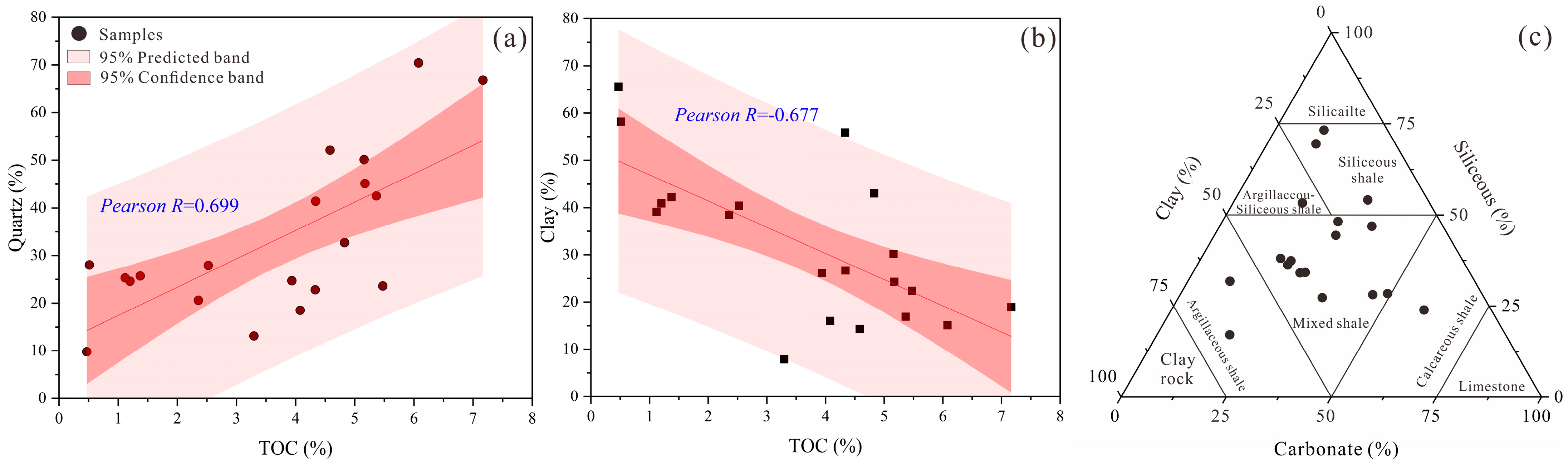
4.1. Geochemical Parameters and Mineral Composition

X-ray diffraction (XRD) analysis of the Wufeng–Longmaxi shale revealed its composition to be predominantly quartz, feldspar, and OM fragments. The samples from the Longmaxi Formation have a quartz content ranging from 9.8 to 70.4%, with an average of 36.12%, and clay mineral content ranging from 7.9 to 65.6%, averaging 30.13%. Additionally, feldspar (potassium feldspar and plagioclase) is present in the samples, ranging from 1.0 to 7.3%, with an average of 3.7%, while carbonate minerals (calcite and dolomite) range from 4.9 to 73.5%, averaging 26.4%. Pyrite content ranges from 1.6 to 4.7%, averaging 3.2% (

Table 1. Mineral compositions and TOC content of the Longmaxi shale.

Sample ID	Well	Lithofacies	Depth (m)	Quartz (%)	Feldspar (%)	Plagioclase (%)	Calcite (%)	Dolomite (%)	Pyrite (%)	Clar (%)	TOC (%)
M-1	N16	M	2321.9	45.1	1.0	2.1	11.5	12.5	3.0	24.3	5.2
M-2	NX2	M	3920.3	32.7	0.5	4.9	5.4	8.8	4.7	43.0	4.8
M-3	NX2	M	3926.8	41.4	0.4	2.6	6.6	17.9	4.4	26.7	4.3
Q-1	N11	Q	2346.2	70.4	0.8	2.1	4.7	4.7	1.7	15.1	6.1
Q-2	NX2	Q	3923.3	52.1		2.0	9.5	19.6	2.5	14.3	4.6
Q-3	NX2	Q	3923.3	50.1	0.5	2.7	4.2	7.7	4.6	30.2	5.2
A-1	N16	A	2290.7	9.8	2.9	4.4	7.2	7.7	2.1	65.6	0.5
A-2	NX2	A	3812.7	28.0		3.8	4.9		1.6	58.2	0.5
C-1	N16	C	2322.4	18.5	1.4	4.0	36.2	21.1	2.6	16.0	4.1
C-2	NX2	C	3941.7	13.1		1.0	27.8	45.7	4.5	7.9	3.3

).

The lower part of the Longmaxi Formation is an anoxic reduction environment with a high presence of graptolites and microorganisms. Zhao et al. [60] conducted significant and trace element analysis of shale in the Sichuan Basin and concluded that most of the siliceous material in the shale originates from late-stage biocement, such as radiolaria, with a high silicon content, rather than clastic quartz. The high TOC content (>3.00%) and quartz content (>46.0%) in the samples are consistent with this result. The strong positive correlation between TOC and quartz content (Figure 2a) suggests that the TOC content is closely related to the development of large amounts of biogenic silica. This finding is in line with previous research [11,60] that revealed a strong positive correlation between TOC content and clay content (Figure 2b). Using the previous “three-terminal” mineral fraction petrographic scheme, the 10 shale samples were classified into four main phases: siliceous shale, argillaceous shale, calcareous shale, and mixed shale (Figure 2c).

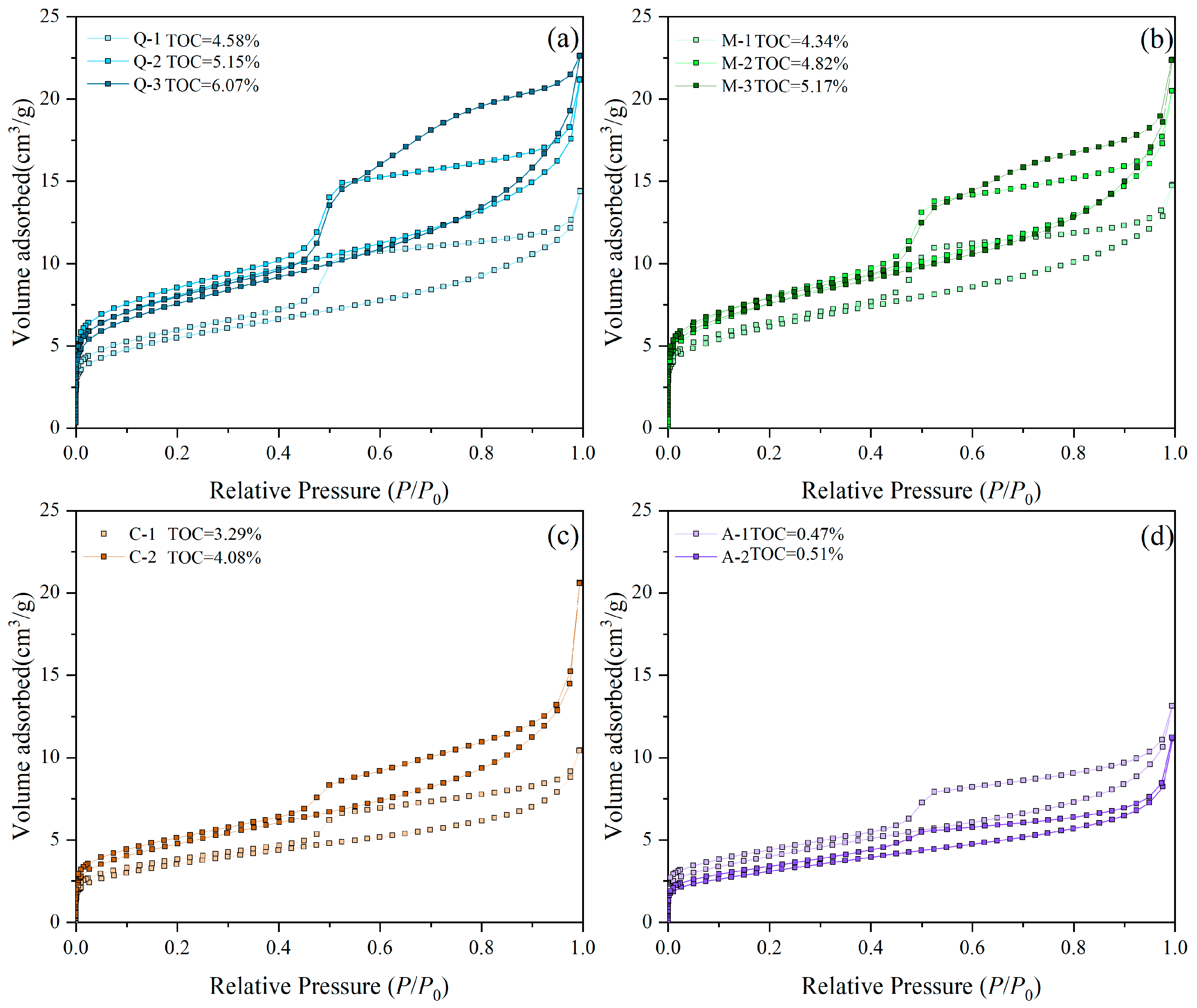
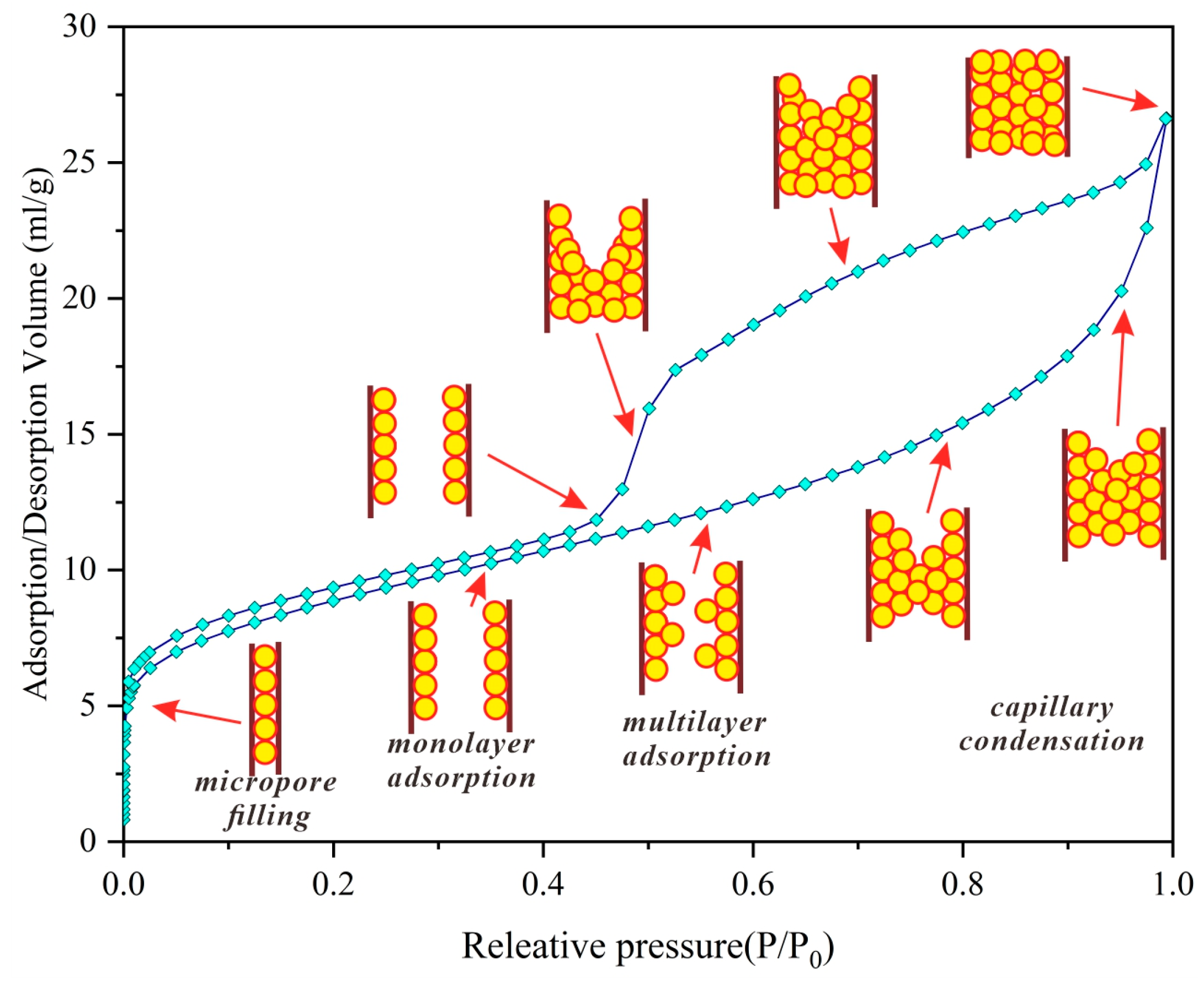
4.2. Adsorption–Desorption Isothermal Diagrams

Low-pressure nitrogen adsorption is mainly used to characterize meso-macropore characteristics. Figure 3 shows that the nitrogen adsorption and desorption curves with all shale samples are more obviously different from lithofacies. For different lithofacies, the TOC content has a more obvious control on the maximum adsorption capacity of shale when the relative pressure is close to 1. There is a pattern that the maximum adsorption gas content increases with increasing TOC content in different lithofacies.

Low-pressure nitrogen adsorption is a widely used method to characterize meso-macropore features in shale. As shown in Figure 3, the nitrogen adsorption and desorption curves for all shale samples are distinctly different from each lithofacies. For each lithofacies, the maximum adsorption capacity of shale is highly dependent on its TOC content when the relative pressure is nearly 1. It is observed that the maximum adsorption gas content increases with the increase in TOC content for different lithofacies. The branch of the N₂ adsorption curve indicates that the curve is slightly convex upward (the relative pressure ≈ 0.2), which represents the saturated adsorption capacity of monolayer molecules [41]. As pressure increases, multi-molecular layer adsorption occurs, and the adsorption capacity increases slowly [64]. At high relative pressures (≈0.8), adsorption rises sharply and does not show adsorption saturation until it is near the saturated vapor pressure, indicating the presence of mesopores and macropores in the sample. When the relative pressure reaches 0.9~1.0, the large pore volume is filled with capillary condensation (Figure 4). Due to the tensile effect, the desorption branch on the outer surface does not coincide with the adsorption branch, and a hysteresis loop appears [40,64].

According to the IUPAC classification, the isothermal adsorption–desorption line curves belong to type IV, indicating the development of mesopores and open pores during multilayer adsorption in shales [77,78]. The steeper slope of the isotherm at the inflection point indicates a narrower PSD and smaller relative pressure. Moreover, the typical hysteresis loops were observed in all samples, which belong to H2 and H3 types, indicating that the pore space is mainly dominated by ink-bottle and parallel-plate pore space [17,78]. The hysteresis loops vary in different lithofacies; Q and M lithofacies are dominated by type H2, indicating ink-bottle-type, tubular pore structures, while C and A lithofacies are dominated by type H3, indicating narrow fracture-like pores between parallel walls.

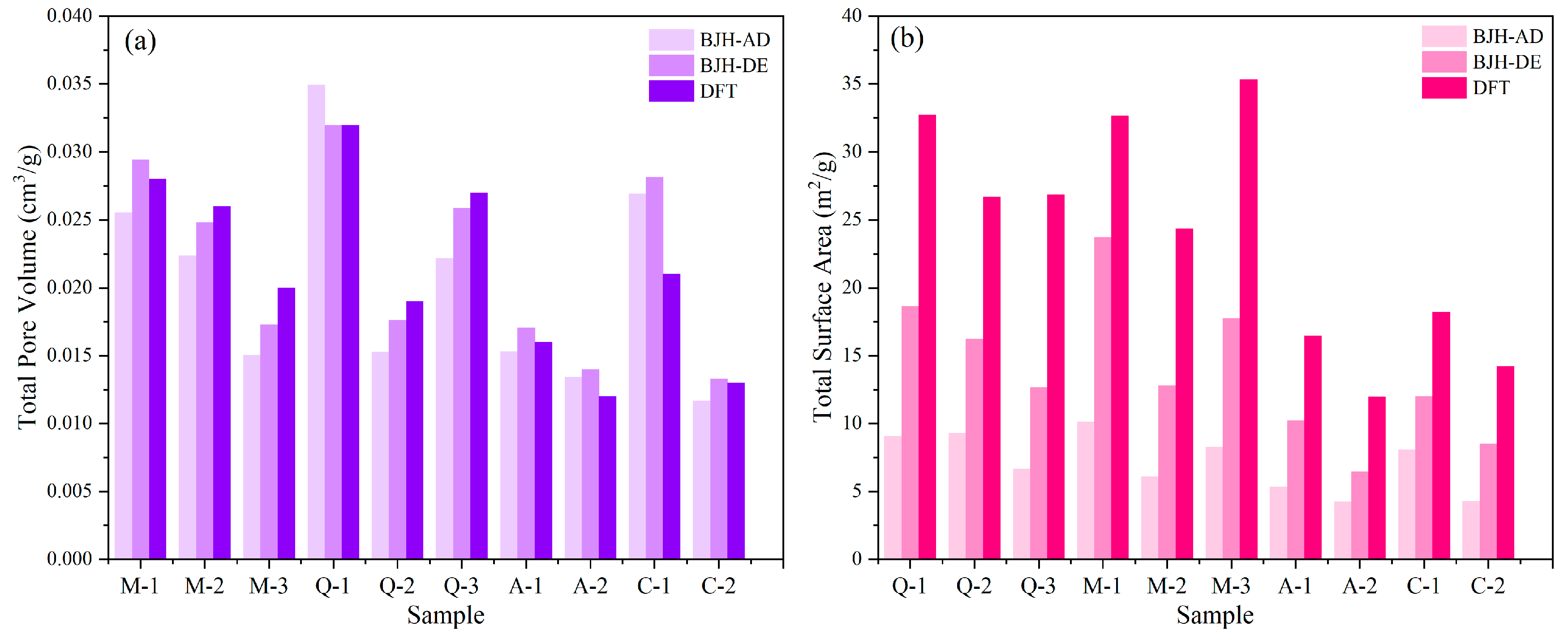
4.3. Pore Structure Parameters from Different Methods

The pore structure was analyzed from N₂ adsorption isotherms based on the BJH (BJH-AD and BJH-DE) and DFT models. From

Table 2. Surface area of the shale samples by the various methods.

Number	BJH (m2/g)		DFT (m2/g)	MultiPoint BET (m2/g)	t-plot External (m2/g)	Langmuir Surface Area (m2/g)
	Adsorption	Desorption
M-1	9.065	18.62	32.741	27	15.78	22.65
M-2	9.286	16.22	26.689	27.12	17.26	21.78
M-3	6.658	12.66	26.837	21.99	12.58	18.4
Q-1	10.1	23.73	32.658	27.1	17.17	22.05
Q-2	6.082	12.8	24.35	19.69	11.88	16.18
Q-3	8.261	17.76	35.34	28.8	16.11	24.08
A-1	5.336	10.22	16.446	14.39	10.36	11.57
A-2	4.251	6.44	11.986	11.17	8.675	8.572
C-1	8.079	12	18.195	17.12	13.84	12.73
C-2	4.266	8.505	14.197	12.69	8.562	9.501

and

Table 3. Pore volume of the shale samples by the various methods.

Number	BJH (m2/g)		DFT Pore Volume (cm3/g)	t-Method Micropore Volume (cm3/g)	Micropore Volume (cm3/g)
	Adsorption Pore Volume	Desorption Pore Volume			HK Method	SF Method
M-1	0.0255	0.0294	0.0280	0.0050	0.0111	0.0346
M-2	0.0224	0.0248	0.0260	0.0045	0.0045	0.0317
M-3	0.0150	0.0173	0.0200	0.0043	0.0090	0.0229
Q-1	0.0350	0.0320	0.0320	0.0044	0.0111	0.0350
Q-2	0.0153	0.0176	0.0190	0.0035	0.0080	0.0223
Q-3	0.0222	0.0259	0.0270	0.0058	0.0118	0.0328
A-1	0.0153	0.0171	0.0160	0.0020	0.0057	0.0203
A-2	0.0134	0.0140	0.0120	0.0012	0.0044	0.0172
C-1	0.0269	0.0282	0.0210	0.0015	0.0069	0.0319
C-2	0.0117	0.0133	0.0130	0.0019	0.0051	0.0162

, the results of the SA and PV calculations are different for BJH and DFT models. In terms of pore volume, the PV of the BJH-AD, BJH-DE, and DFT models in mixed and siliceous lithofacies obtained using N₂ adsorption data were 0.0150–0.0350 cm³/g, 0.0173–0.0320 cm³/g, and 0.0190–0.0320 cm³/g, respectively (Table 2). The results showed that the average pore volumes of the DFT model were larger than those of the BJH-AD and BJH-DE in most mixed and siliceous lithofacies. However, this trend is not obvious in the argillaceous and calcareous lithofacies (Figure 5a). This is mainly due to the wider measurement range of the DFT model, which can measure more micropores. Meanwhile, the siliceous shale and mixed shale contain more micropores, showing that the pore volume of the nitrogen adsorption model was calculated following the DFT > BJH.

Figure 5b shows that the pore surface area of each sample follows the trends DFT > BJH-DE > BJH-AD. Compared with the argillaceous and calcareous lithofacies, the siliceous and mixed shale lithofacies have a higher pore surface area. The SA of N₂ adsorption calculated by the BJH-AD model and DFT model is 4.25–10.10 m²/g and 11.99–35.34 m²/g, respectively, while that of the BJH-DE model is 6.44–23.73 m²/g (Table 3). For siliceous and mixed lithofacies, the PV of the DFT model is about 2.87–4.28 times that of the BJH-AD model, and the PV of the BJH-DE model is about 1.75–2.15 times that of the BJH-AD model. The SA of the samples calculated using the DFT model is more significant than those calculated using the BJH-DE and BJH-AD models (Figure 5b). The values of the pore structure parameters calculated by the three models followed the rule of DFT > BJH-DE > BJH-AD.

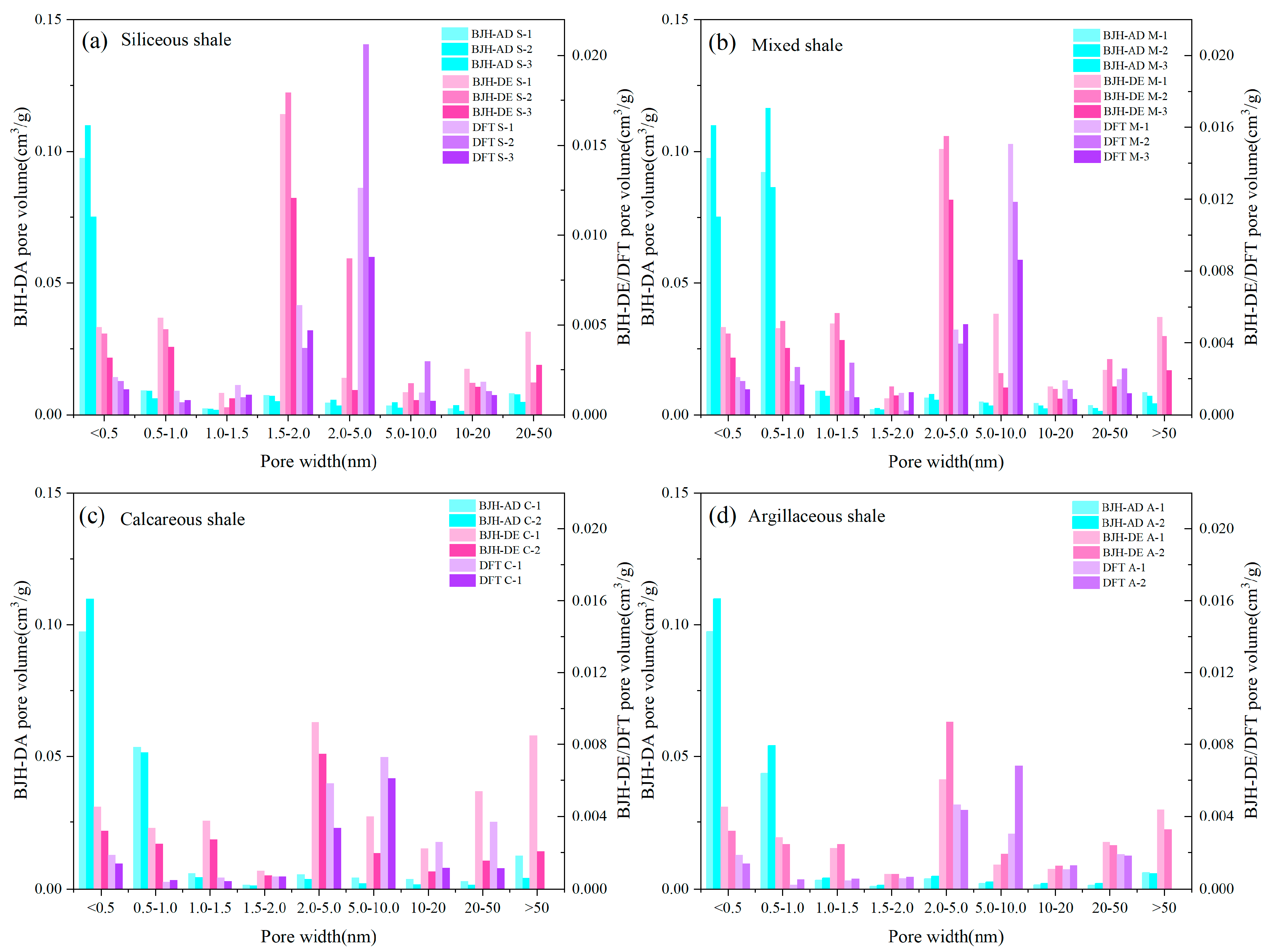
4.4. Pore Size Distribution from Different Methods

Figure 6 illustrates the comparison of the PSD results obtained from the BJH-AD, BJH-DE, and DFT adsorption models for the same sample. The curve of nitrogen adsorption for this sample is also presented in the figure. The PSD curves derived from BJH-AD, BJH-DE, and DFT exhibit a multimodal characteristic. However, the calculated PSD curves obtained from these models do not overlap, indicating the impact of utilizing different models on the results. Notably, the BJH-DE model shows an abnormally high value at a diameter of 3.8 nm, which is not observed in DFT and BJH-AD models. This phenomenon is suggested to be an artificial peak caused by the presence of ink-bottle-type pores in the sample. These artificial peaks mainly result from tensile strength effects, where large pores desorb first when the pressure drops, and small pores desorb when the pressure reaches the required threshold [35,36,79]. When the relative pressure is reduced to the range of 0.45 to 0.55 (threshold reached), the tensile strength effect causes capillary evaporation to reach the minimum pore pressure, leading to a sudden decrease in the amount of adsorption on the desorption branch [80]. This effect results in narrower pore size distribution with significant peak values obtained from the BJH-DE model calculations, which may lead to errors in the data. Several factors may account for this phenomenon, including the separation of the adsorbed film and the capillary condensate by the BJH model, the overlook of fluid–wall interactions that significantly affect the adsorbate behavior in the pores, and the reliance of the BJH model on the Kelvin equation, which is not applicable in extremely narrow pores, as noted by Rouquerol et al. [27].

The shale develops many micropores and mesopores, and SEM observations show that the shale develops many ink-bottle-shaped pores with a high probability of TSE [77,78]. Therefore, for shale reservoirs, desorption branches are not often used in calculating PSD. The PSD curves of the BJH model are smoother than other PSD models, while the PSD curves of the DFT model show multi-peaked features.

Pores with smaller diameters can be detected using the DFT model, which is not detected by the BJH-AD and BJH-DE methods. The BJH-AD curve is higher than the DFT model curve at less than 0.8 nm, while the DFT model is significantly higher than the BJH-AD at pore diameters greater than 0.8 nm and shows multiple peaks at 1–10 nm. By studying the DFT model, Li et al. [35] found that the multi-peak phenomenon in the PSD gradually disappeared as the number of large pores decreased, and the number of small pores increased. This confirms that the DFT model may prefer to describe the micropore size distribution, such as micropores or narrow mesopores.

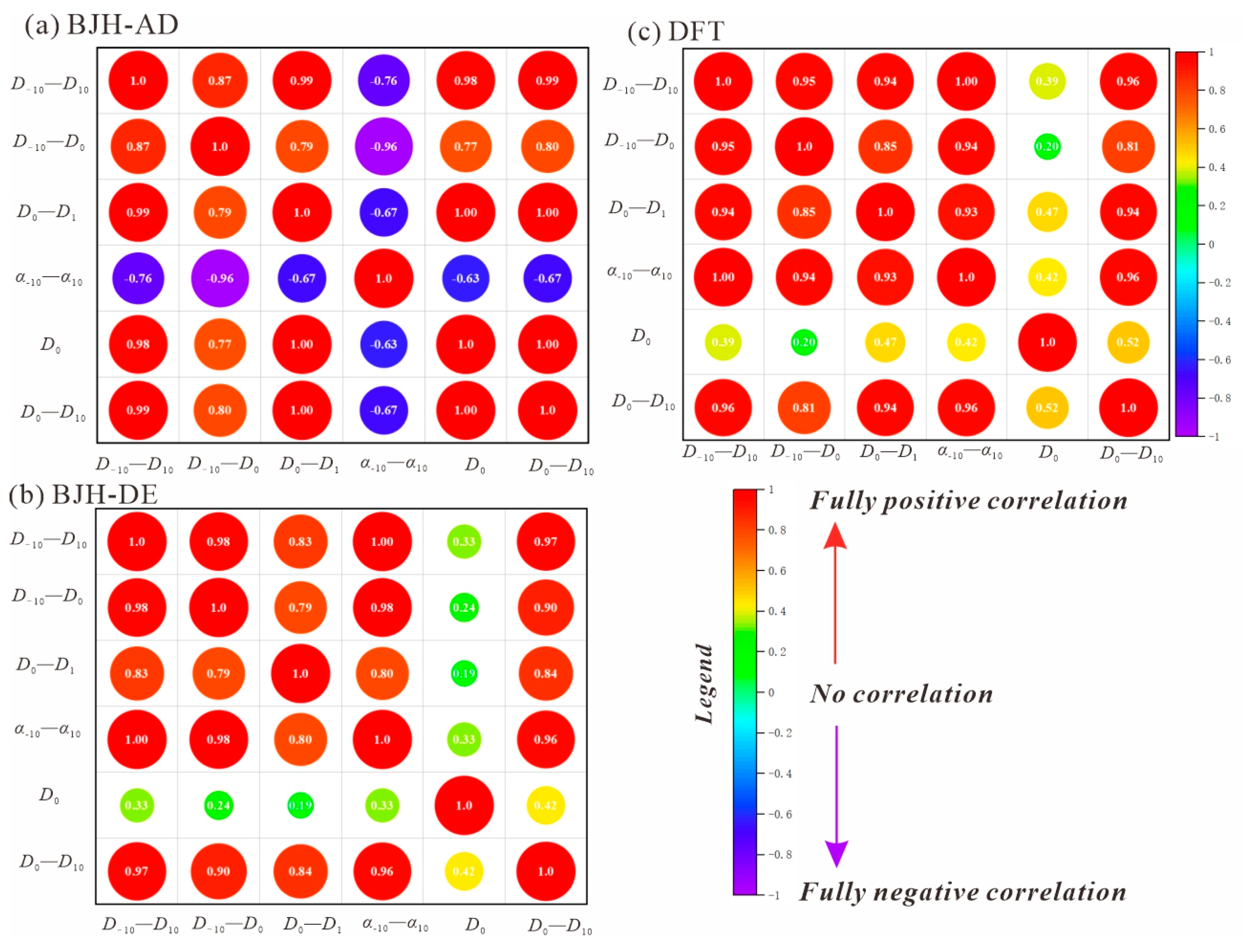
4.5. Multifractal Characteristics from Different Methods

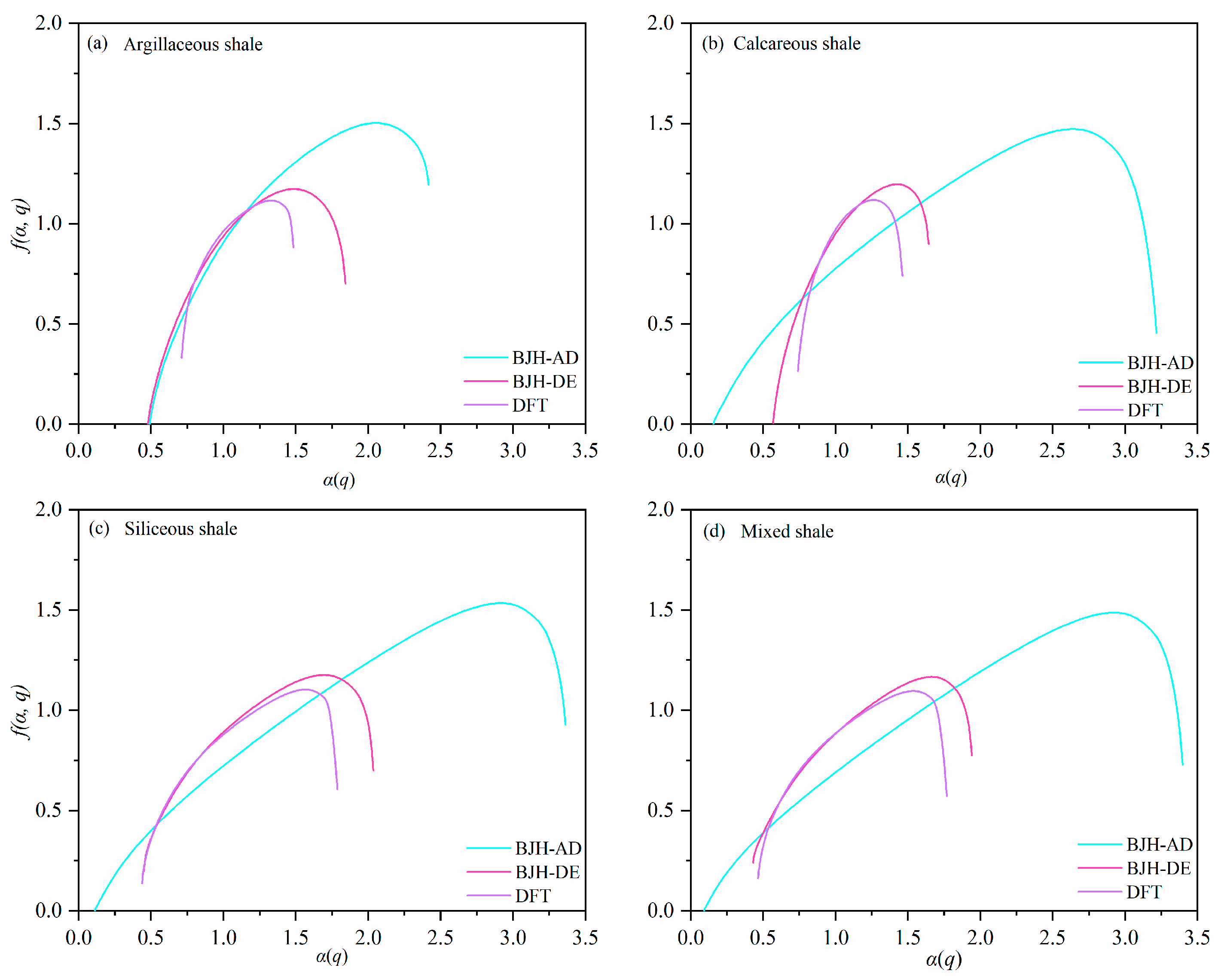
4.5.1. Multifractal Spectra from Different Methods

In this paper, the multifractal calculations of three nitrogen adsorption models, BJH-AD, BJH-DE and DFT, are carried out for different shale lithofacies, where the parameter q is taken to be in the range (−10, 10) with the value interval 1. Figure 7, Figure 8 and Figure 9 and

Table 4. Multifractal analysis results of the samples using BJH-DE, BJH-DE, and DFT models.

Sample ID	Model	D−10–D10	D10–D0	D0–D10	D1/D0	D2	D1	D0	D−10	D10	Δα	Δf	Hurst
M-1	BJH-AD	2.793	1.391	1.402	0.392	0.302	0.618	1.575	2.966	1.575	3.062	0.456	0.651
M-2		2.938	1.477	1.462	0.296	0.197	0.466	1.572	3.049	1.572	3.186	0.679	0.598
M-3		3.055	1.569	1.486	0.270	0.177	0.428	1.585	3.154	1.585	3.307	0.728	0.588
Q-1		2.751	1.319	1.432	0.343	0.244	0.537	1.569	2.888	1.569	2.983	0.700	0.622
Q-2		3.018	1.509	1.509	0.307	0.217	0.501	1.631	3.140	1.631	3.252	0.928	0.608
Q-3		3.036	1.594	1.442	0.297	0.231	0.466	1.572	3.166	1.572	3.352	0.131	0.615
A-1		2.760	1.347	1.413	0.382	0.282	0.600	1.572	2.920	1.572	3.021	0.473	0.641
A-2		1.760	0.733	1.027	0.723	0.845	1.136	1.572	2.305	1.572	1.925	1.193	0.923
C-1		2.793	1.391	1.402	0.392	0.302	0.618	1.575	2.966	1.575	3.062	0.456	0.651
C-2		1.760	0.733	1.027	0.723	0.845	1.136	1.572	2.305	1.572	1.925	1.193	0.923
M-1	BJH-DE	1.320	0.657	0.664	0.772	0.749	0.939	1.216	1.872	1.110	1.547	−0.051	0.874
M-2		1.716	0.776	0.940	0.724	0.914	1.168	1.613	2.388	1.535	1.906	1.007	0.957
M-3		1.384	0.616	0.768	0.496	0.584	0.605	1.219	1.835	0.981	1.511	0.536	0.792
Q-1		1.400	0.743	0.657	0.763	0.744	0.926	1.213	1.956	1.074	1.636	−0.126	0.872
Q-2		1.436	0.679	0.757	0.674	0.626	0.832	1.236	1.915	1.037	1.585	0.500	0.813
Q-3		1.328	0.614	0.714	0.686	0.647	0.839	1.222	1.836	0.966	1.452	0.600	0.823
A-1		1.921	0.971	0.951	0.528	0.437	0.647	1.224	2.194	1.224	2.090	0.783	0.718
A-2		1.207	0.516	0.691	0.805	0.799	0.984	1.222	1.738	1.222	1.364	0.700	0.899
C-1		0.943	0.345	0.598	0.850	0.886	1.045	1.230	1.575	1.224	1.073	0.893	0.943
C-2		0.377	0.141	0.236	0.959	1.126	1.176	1.227	1.368	0.688	0.452	0.528	1.063
M-1	DFT	0.932	0.348	0.584	0.809	0.771	0.924	1.142	1.490	1.030	1.057	0.571	0.885
M-2		1.389	0.549	0.839	0.641	0.537	0.769	1.200	1.750	1.198	1.594	0.052	0.769
M-3		1.161	0.525	0.636	0.702	0.646	0.797	1.135	1.660	0.974	1.304	0.411	0.823
Q-1		1.240	0.614	0.626	0.760	0.706	0.864	1.137	1.751	1.072	1.423	0.301	0.853
Q-2		1.210	0.537	0.673	0.688	0.624	0.786	1.143	1.680	1.007	1.350	0.469	0.812
Q-3		1.166	0.499	0.667	0.693	0.619	0.783	1.131	1.629	1.037	1.294	0.628	0.810
A-1		0.923	0.348	0.575	0.809	0.771	0.924	1.142	1.490	1.084	1.054	0.625	0.885
A-2		0.675	0.286	0.389	0.857	0.876	0.979	1.142	1.428	0.811	0.772	0.550	0.938
C-1		0.603	0.254	0.349	0.905	0.949	1.034	1.142	1.396	0.878	0.721	0.476	0.974
C-2		0.995	0.395	0.600	0.796	0.742	0.905	1.138	1.533	1.069	1.132	0.558	0.871

show the mass index, generalized fractal dimension, and multiple fractal singularity spectra for the three nitrogen adsorption models, respectively. Previous authors have identified three conditions that need to be satisfied for multiple fractal results in porous media [16,25,26,37,38,55,56]: (1) the mass index τ(q) is strictly monotonically increasing with q; (2) D_q is strictly monotonically decreasing with q; and (3) f(α) has a convex function with α. The different nitrogen adsorption model curves all satisfy these three conditions, indicating that they all fit the multifractal profile [16,25,26,37,38,55,56].

The mass index spectrum is a widely used method to assess whether an object has multifractal characteristics. If the mass index τ(q) increases monotonically as q increases, then the object exhibits a multifractal character (Figure 7). In all three models shown in Figure 7, τ(q) grows monotonically and can be divided into two phases: a rapid growth phase for q < 0 and a slower growth phase for q > 0. The τ(q) values for BJH-AD are smaller compared to the other models, whereas the values for DFT and BJH-DE are more similar.

Figure 8 shows the multiple fractal singularity spectra of the three gas adsorption models. These curves have an asymmetric convex shape. In the left-hand branch, f(α) corresponding to the high probability measurement region increases sharply with α, whereas the opposite is true in the right-hand branch in the low probability measurement region. The results of previous studies show that the left-hand branch indicates the singular intensity in the region of high probability measurements, and the right-hand branch indicates the singular intensity in the region of low probability measurements. The difference in the curve α(q) is the multiple fractal singular spectrum width, which describes the local characteristics of the pores in terms of fractal structure and represents the PSD with different diameters [25,26,38]. The results show that the multifractal spectral curves of the three N₂ adsorption calculation models show a predominance of large pores. The BJH-AD model has a more heterogeneous and not uniform PSD than the DFT and BJH-DE models.

Figure 9 shows the generalized dimensional spectral function for the three gas sorption models, with Dq showing a clear monotonical decrease with q. When q > 0, Dq decreases rapidly; while q < 0, Dq tends to decrease slowly, a result similar to the results of previous studies of the Barnett Shale [25,26,38]. The q > 0 segment represents the pore characteristics of the high probability measurement interval, while the q < 0 segment represents the pore characteristics of the low probability measurement interval; the DFT model is higher than the BJH-AD and BJH-DE models. In the q > 0 segment, the difference between the three gas adsorption models is not significant [25,38]. The higher curvature of the mass index spectrum curve, the greater the concentration of the PSD [56]. The curvature of the BJH-AD, BJH-DE, and DFT models decreases in turn, indicating that the BJH-AD model has a high non-homogeneity of the local PSD, while the DFT model has a weak non-homogeneity of the PSD curve.

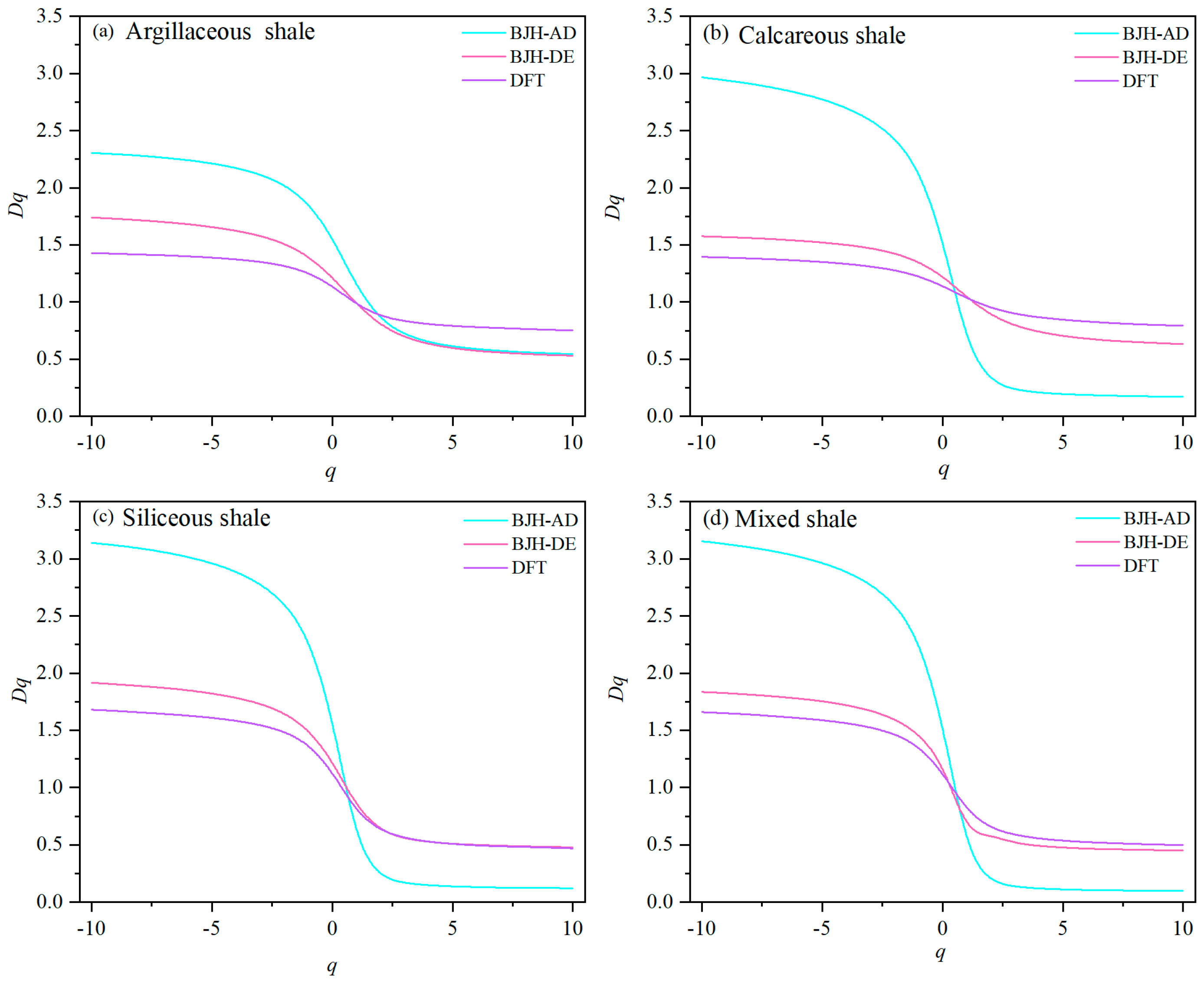
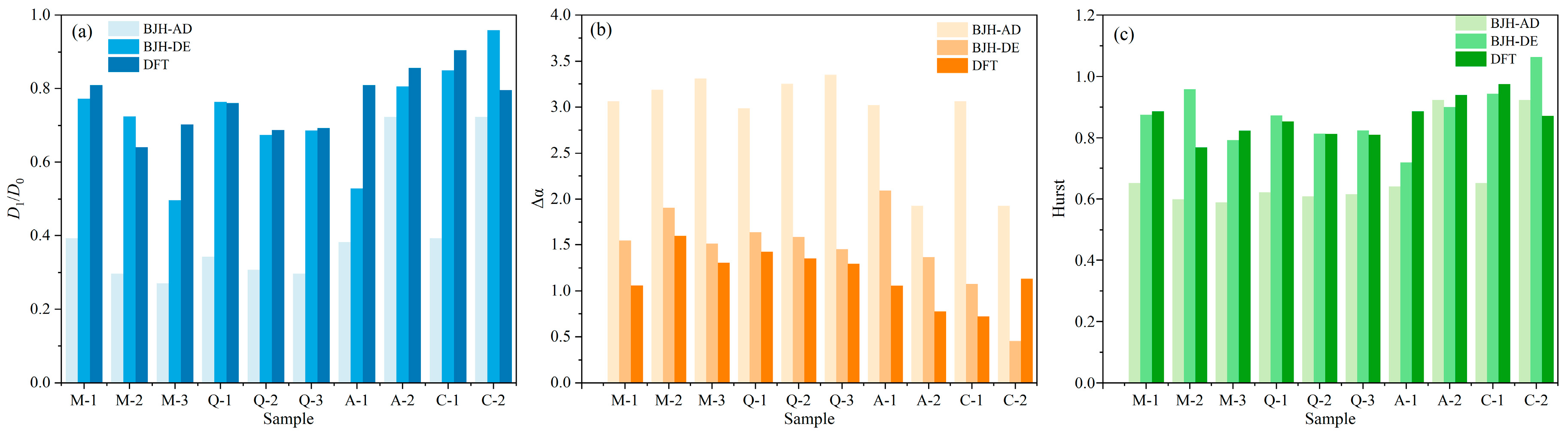
4.5.2. Multifractal Parameters from Different Methods

According to multifractal theory, a larger capacity dimension (D₀) indicates a wider range of power spectral density (PSD) in shale reservoirs, while the information entropy dimension (D₁) reflects the degree of concentration of PSD measures, which characterizes the degree of inhomogeneity. A larger D₁ suggests a broader range of PSD in the reservoir and uniform distribution of pore volume percentages for different pore sizes. D₁/D₀ describes the degree of dispersion of the shale PSD. In Figure 10a, the BJH-AD values are much lower than those of the BJH-DE and DFT models, indicating that the BJH-AD pore volumes are less discrete and mainly clustered in the same pore size range. The width of the multifractal spectrum Δα, which is the difference between the maximum and minimum values of the α parameter, reflects the non-uniformity of the distribution of probability measures of physical quantities across the fractal structure. A larger Δα indicates a more inhomogeneous PSD and a more non-homogeneous pore structure. The results show that the BJH-AD model has the strongest non-homogeneity in calculating the pore structure, with Δα values higher than those of the BJH-DE and DFT models, indicating that the BJH-AD model has the most non-uniform PSD (Figure 10b). For Δα values, the three nitrogen adsorption models follow the pattern BJH-AD > DFT > BJH-DE.

The Hurst exponent, which measures the self-affinity of signals and is also known as the roughness exponent, can be generalized to generalized fractal dimension D [81]. It quantifies the relative tendency of a porosity series either to regress strongly to the mean or to cluster in a direction. For PSD, the Hurst(H) index indicates the degree of positive autocorrelation, defined previously as H = (D₂ + 1)/2, with a range of variation between 0.5 and 1. In this case, smaller (1-H) values indicate a higher degree of positive autocorrelation in the size-dependent distribution of any property. A value of H in the range of 0.5–1 indicates a porosity series with long-term positive autocorrelation, meaning that both a high value in the series will probably be followed by another high value and that the values in a porosity series in the future will also tend to be high. The results show that the mean value of (1-H) for BJH-AD is 0.318, which is lower than the mean values for BJH-DE and DFT, indicating that the model has the highest autocorrelation among the different pore size distributions, consistent with the results for the degree of non-homogeneity of the PSD (Figure 10c). The Hurst index can also be used to specify pore connectivity on networks of different pore sizes, indicating differences in the permeability of the samples. A smaller Hurst index value indicates poorer pore connectivity. The mean value of Hurst for BJH-AD is 0.682, which is lower than the mean value of BJH-DE (0.8754) and the mean value of DFT (0.862), indicating a poor distribution of shale pore connectivity under this model, with the BJH-DE and DFT model calculations having more similar results.

5. Discussion

5.1. Comparison of BJH and DFT in Pore Characterization

In this section, we compare and analyze the differences in pore volume distribution obtained from various nitrogen adsorption models. The principle of the density functional theory (DFT) is based on the behavior of fluid molecules in confined spaces. The Barrett–Joyner–Halenda (BJH) analysis method uses the modified Kelvin equation of the macroscopic thermodynamic principle to calculate the PSD. Figure 11 shows that the DFT model exhibits multi-peak characteristics, while the BJH-AD model pore volume is concentrated mainly in two ranges (<0.5 nm and 0.5–1.0 nm). In contrast, the BJH-DE model peak is in the 2.0–5.0 nm pore range. This phenomenon has attracted attention in the study of shale PSD characteristics. Scholars have investigated the differences between PSDs from N₂ adsorption and desorption data [82]. However, it is unclear which data to choose during PSD calculation.

Recent research suggests a peak at 3.8 nm in the shale PSD curve obtained using the BJH-DE model, which was initially interpreted as a rock characteristic. However, the interpretation of the tensile strength effect has been accepted over the past few years. The shale has considerable ink-bottle-like pores, and the large pores first undergo desorption in the gas desorption process. When the relative pressure reaches the critical value, the capillary condensation phenomenon disappears, and the N₂ desorption amount suddenly increases. This results in the desorption isotherm decreasing suddenly, leading to a significant mutation point of the gas desorption curve and a false peak on the PSD curve. Most pores in this study had complex structures and were ink-bottle-like, and the BJH-DE model showed an abnormally high peak at 3.8 nm. Therefore, the results suggest that the desorption branch of N₂ should not be used to calculate shale pore structure parameters.

The validity of the Kelvin equation for adsorption branches is unclear because numerous narrow mesopores in shale make the fluid–pore wall interaction dominate the adsorption process. Some scholars investigated typical mesoporous molecular sieves using the BJH model with XRD and TEM and suggested that the BJH method and the relevant Kelvin equation program may underestimate pore size by 20 to 30% without proper correction for narrow mesopores less than nearly 10 nm. Although some scholars have begun to calibrate the Kelvin equation using the known pore size of mesoporous molecular sieves, this equation still has a limited scope of application. Additionally, the classical BJH method does not consider the effect of adsorption potential on the pore condensation transition position and assumes that the pore fluid has the same thermodynamic properties as the corresponding volume fluid. Therefore, the BJH-AD model’s erroneous assumptions may underestimate some pores (<10 nm) in shale.

The Kelvin method does not consider the effect of adsorption force on pore condensation and does not express the basic mechanism of pore condensation and hysteresis (due to the occurrence of delayed condensation arising from metastable pore fluid), which the DFT model addresses. The DFT method obtains the thermodynamics and density distribution of the fluid, expresses the adsorption process at the molecular scale, and correctly characterizes the local fluid structure near the curved solid wall at the micro level without considering the effect of the hysteresis loop. Existing research suggests that for mesoporous molecular sieves, the average pore size obtained using the adsorption and desorption curves is consistent. Therefore, the DFT method correctly characterizes the local fluid structure near the curved solid wall at the micro level without considering the effect of the hysteresis loop [29,71].

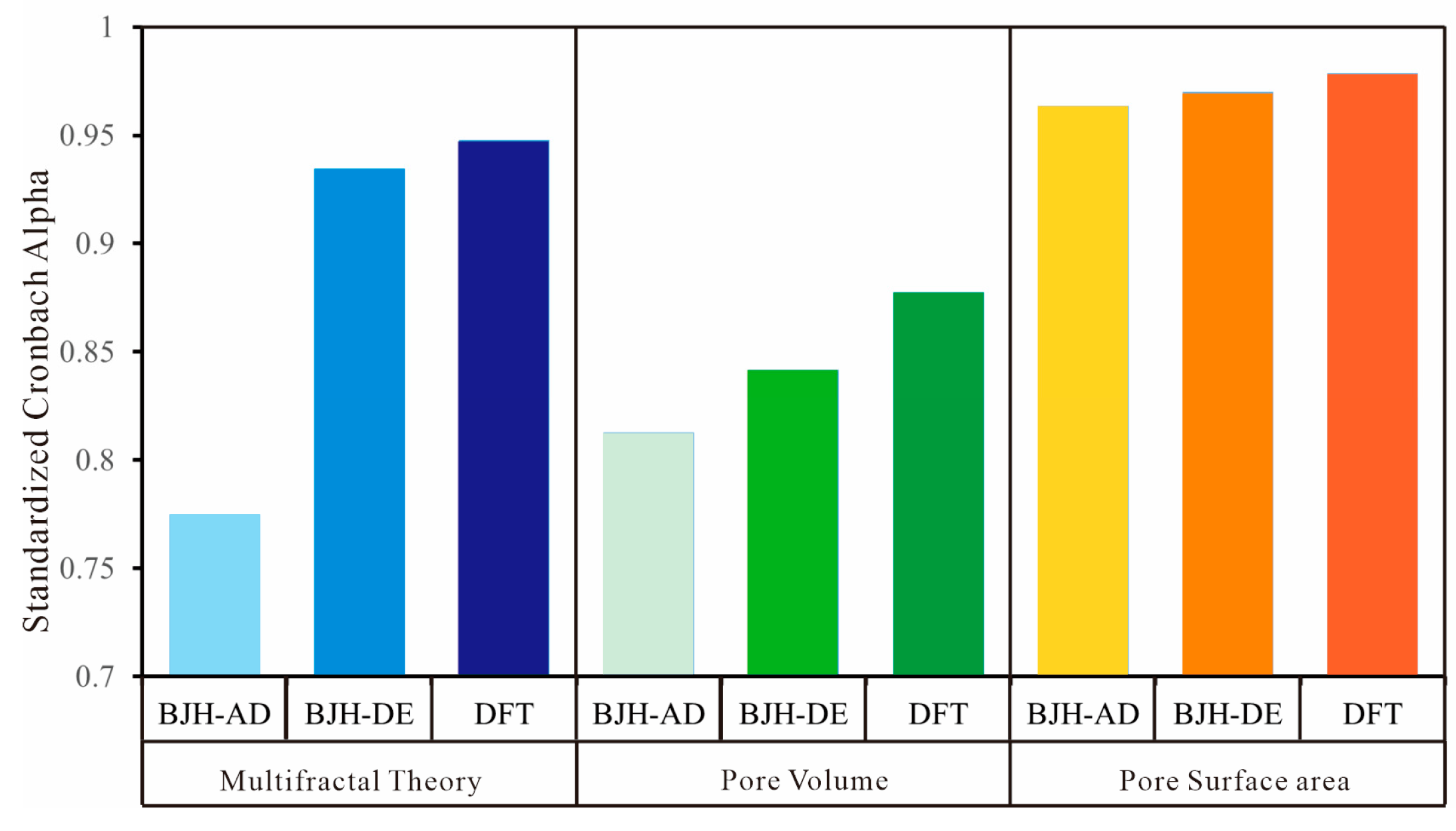
5.2. Model Selection and Comparison

As mentioned in Section 4.4, significant differences were identified in the PSD obtained using different nitrogen adsorption models, primarily due to the difference in the calculation principles of the BJH and DFT models, as well as the complex internal pore structure of shale (e.g., various pore morphologies), thus resulting in different calculation results. The BJH model originated from the Kelvin equation of macro thermodynamics. For the adsorption curve, the macroscopic thermodynamic model cannot apply to the microstructure characterization (due to the unstable cylindrical meniscus during the adsorption), and the adsorption potential affected the pores and caused errors in the calculation results. For the desorption curve, since the pores inside the shale were primarily ink bottles, the multilayer adsorbed gas exhibited a metastable state, thus causing a delay in condensation. There were two states for the hysteresis adsorption branch of the ink-bottle pores simultaneously (including gas–liquid phase transition and reversible liquid–gas phase transition), which did not reach the thermodynamic equilibrium state. The PSD obtained by analyzing the desorption branches artificially made the hole volume unusually high within a specific pore size range [32]. The DFT model characterized the structure of adsorbed molecules in pores at the molecular level, thus avoiding the limitations of the Kelvin equation while describing the interaction between confined fluids and the effect of adsorption potential more specifically [71]. There were ink-bottle pores with a pore diameter of only 5–6 nm inside the shale, and the DFT model considered the correct pore geometry and the presence of metastable pore fluids associated with the pore condensation process. The mixed DFT kernel was applied to the adsorption branch of the isotherm, and the condensation delay was correctly considered. The micro-mesoporous PSD (metastably adsorbed NLDFT kernel) was obtained, thus revealing that the DFT model can better characterize the mesoporous characteristics of shale [64]. Figure 12 presents the correlation between the average pore size and the corresponding pore volume determined using the BJH adsorption method, the BJH desorption method, and the DFT method. The results indicated that the R² value of the DFT model was larger than that of the BJH (adsorption and desorption) model (Figure 12, R²_DFT > R²_BJH), thus also revealing that the DFT method is more suitable for characterizing the PSD of mesopores and macropores.

Since the multifractal theory is capable of obtaining different parameters relating to heterogeneity, various parameters were extracted in this study for the generalized fractal dimension spectrum (e.g., D₋₁₀–D₁₀, D₀–D₁₀, D₋₁₀–D₀, D₋₁₀, D₁₀, Δf, Δα, Hurst). The comparison of the Pearson correlation coefficient matrix of different calculation models indicated that there were different correlations between the multifractal parameters of different models. For the BJH-AD model, except for parameters Δf and Hurst, other parameters had a strong positive correlation, and the coefficients were primarily higher than 0.70. As depicted in Figure 13, parameters D₋₁₀–D₁₀, D₀–D₁₀, D₋₁₀–D₀, and Δα showed a positive correlation, thus suggesting that the generalized dimension spectrum q-D_q is easier to express the multifractal behavior of porous media pore structure than multifractal singular spectrum α-f(α) [83]. Meanwhile, the BJH-DE and DFT models had similar Pearson correlation matrixes. The D₀ parameter is clearly related to the multifractal dimensions; however, the other parameters are more clearly related. A positive correlation was identified between D₋₁₀–D₁₀, D₀–D₁₀, D₋₁₀–D₀, D₋₁₀, D₁₀, and Δα, and the multifractal dimension spectrum showed a significant positive correlation with the width of the singular spectrum, thus revealing that the generalized fractal dimension spectrum q-D_q and the multifractal dimension spectrum α-f(α) obtained using the BJH-DE and DFT models exhibit high consistency in the multifractal characterization of shale pore structure.

Alpha was developed by Lee Cronbach in 1951 to provide a measure of the internal consistency of a test or scale; it is expressed as a number between 0 and 1 [84]. The test can be used to evaluate the internal consistency of continuous variables, and it has also been commonly used to detect the internal consistency of ordered categorical variables and binary categorical variables [84]. This test method should meet three conditions as follows: (a) the test measures a single factor; (b) the test items have the similarity of statistical coefficients; and (c) there is no correlation between different items. Specifically:

$$\alpha =\frac{N·\overline{c}}{\overline{v}+\left(N-1\right)·\overline{c}}$$

(18)

where α denotes the coefficient of reliability; N is equal to the number of items; $\overline{c}$ represents the average inter-item covariance among the items; and $\overline{v}$ expresses the average variance. In general, the higher the coefficient, the higher the reliability of the tool. In basic research, the reliability should be at least 0.80. Furthermore, in exploratory research, the reliability can only be accepted if it reaches 0.70. A reliability between 0.70 and 0.98 is high, while a reliability below 0.35 is low and should be rejected.

Since different parameters of multifractal dimension had a strong correlation, Cronbach’s alpha was adopted to carry out the consistency test of the BJH-AD, BJH-DE, and DFT models. The results showed that for multifractal parameters such as D₋₁₀–D₁₀, D₀–D₁₀, D₋₁₀–D₀, D₋₁₀, D₁₀, and Δα, the consistency of the BJH-DE and DFT models was the highest (0.70), while that of the BJH-AD model was the lowest (Figure 14). The above results suggest that the multifractal parameters obtained using the BJH-DE and DFT models exhibit high consistency for measuring the degree of pore heterogeneity and can characterize the heterogeneity of shale pore structure more accurately. Likewise, the calculations of different models were conducted for the test samples to obtain the pore volume and pore-specific surface area parameters of the test samples. The pore volume and pore-specific surface area test results of the BJH-AD, BJH-DE, and DFT models were compared. The results indicated that the BJH-DE and DFT models were highly consistent with the calculation results of other parameters relating to other pore volumes/pore surface areas (Figure 14). Thus, it suggests that the DFT model exhibits high representativeness when it is adopted to obtain the pore volume/surface area of different test samples. However, the BJH-DE model was not selected since the BJH-DE model will cause the PSD to form an artificial peak, thus resulting in significant errors. In brief, the multifractal theory and Cronbach’s alpha proved that the DFT model was the optimal model for analyzing the pore structure of shale samples by the nitrogen adsorption method.

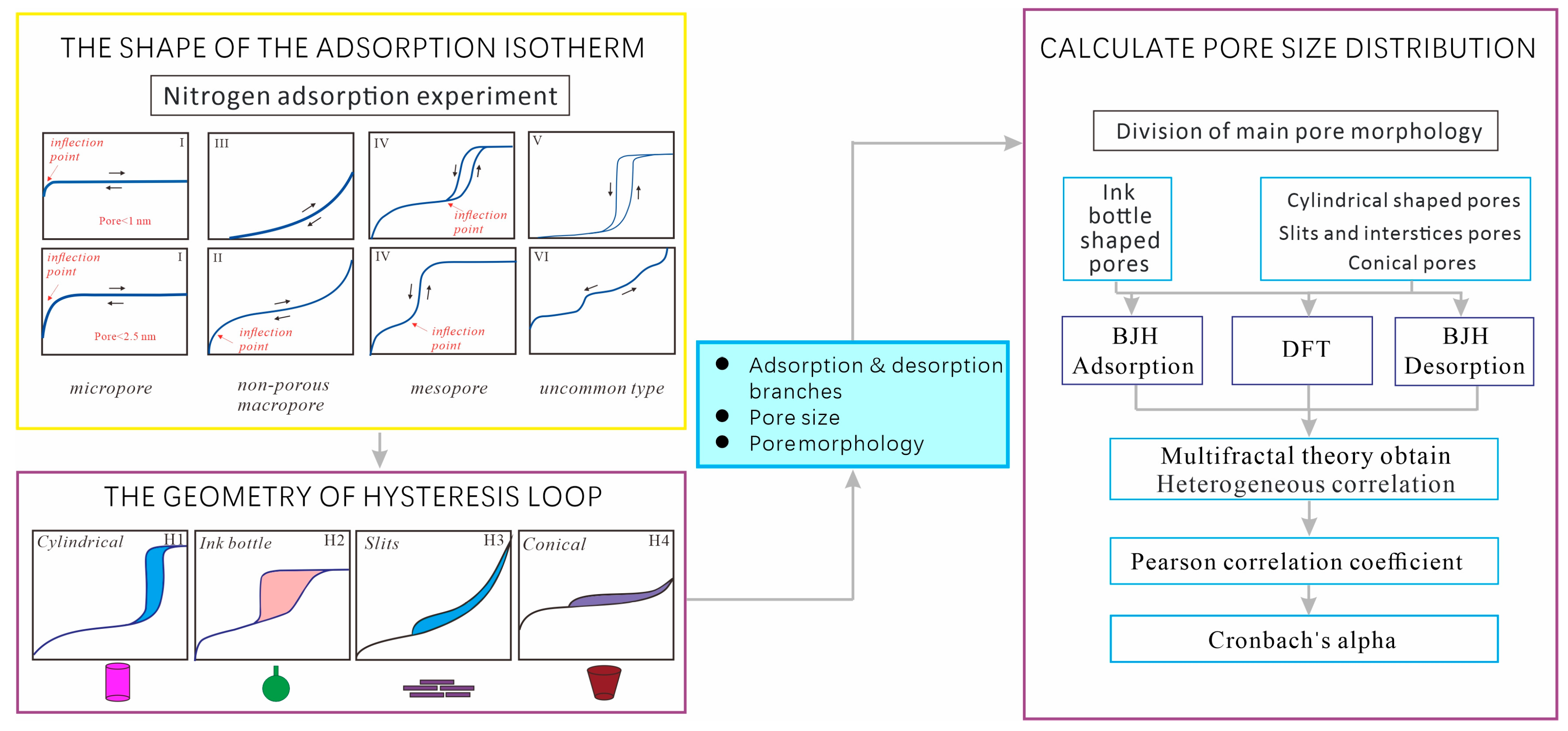
5.3. The Workflow of N₂ Adsorption Method Selection

It has been proved that there are significant errors in the pore structure parameters and the degree of heterogeneity obtained by different calculation models for the isothermal adsorption curve of the same sample. In this study, a specific nitrogen adsorption model calculation and selection process was designed, and it primarily comprised three parts, including adsorption isotherm shape, hysteresis loopback shape, and PSD calculation (Figure 15). First, the pore size should be determined according to the shape of the isotherm after the nitrogen adsorption experiment. The pore size of different samples resulted in significant differences in the isotherm shape, inflection point, and adsorption and desorption curves. For shale reservoirs, nitrogen adsorption experiments were mostly mesoporous, mainly type IV. Next, the characteristics of different hysteresis loop shapes were analyzed, and different hysteresis loop shapes indicated the main pore shapes of the sample. The shale exhibited a complex pore structure, which was often a combination of various hysteresis loops, thus that the classification type should be considered comprehensively. The PSD was obtained based on the experimental nitrogen adsorption and desorption curves and pore characteristics. Since the ink-bottle pores will make the BJH-DE model produce an artificial false peak at 3.8 nm, the ink-bottle pores were separated from the cylindrical and slit pore shapes to calculate the BJH and DFT models, respectively. The multifractal dimensions for the PSD curves were obtained by different models, and the heterogeneity coefficient obtained by multifractals served as the main evaluation parameter to analyze the correlation between different parameters, calculate Cronbach’s alpha, and compare their consistency. The higher the coefficient, the better the calculation model will be to characterize the degree of pore heterogeneity.

In this study, a detailed analysis of the advantages and disadvantages of three nitrogen adsorption modes, namely BJH-AD, BJH-DE, and DFT, was conducted. The adaptability of different sorption models was investigated for the Longmaxi Formation shale in the southern Sichuan Basin, China, with the aim of comparing the calculated results of various nitrogen sorption models and establishing a preference method for nitrogen sorption models. This will enable accurate evaluation of pore size distribution characteristics of shale reservoirs in future studies. However, this paper does not include the quench solid density functional theory (QSDFT) model and non-local density functional theory (NLDFT) model. Additionally, the study overlooks the importance of microporous model selection in analyzing the pore size distribution in shale reservoirs. These shortcomings could be addressed in future research to advance our understanding of the pore structure of shale reservoirs.

6. Conclusions

In this study, the models with different pore size distributions (BJH-AD, BJH-DE, and DFT) were compared for Longmaxi shale samples through nitrogen adsorption experiments. Combining the three different methods with multifractal theory, the consistency of heterogeneity parameters of different nitrogen adsorption models was analyzed using Cronbach’s alpha, and the main conclusions are as follows:

Nitrogen adsorption data were analyzed by different models, and the results revealed that the pore structure parameters obtained by different models were different. When the pore size was less than 0.8 nm, the BJH-AD curve was higher than the DFT model curve. When it was higher than 0.8 nm, the DFT adsorption model was significantly higher than the BJH-AD, and multiple peaks appeared at 1~2 nm, thus suggesting that the DFT model is more capable of characterizing pores with a pore size of about 2 nm than the BJH model. The BJH-DE formed a significant artificial peak near 3.8 nm due to the tensile strength effect.

The nitrogen adsorption curve of the same sample exhibited multifractal characteristics, whereas the multifractal parameters obtained using the three adsorption models were significantly different. The degree of heterogeneity obtained indicated the rule of BJH-DE > DFT > BJH-AD; D₁/D₀ indicated that BJH-AD was the highest, thus revealing that the smaller the degree of dispersion of the model aperture, the more concentrated the PSD will be in the dense interval.

The DFT model is capable of accurately characterizing the structure of adsorbed molecules in pores at the molecular level using N₂ adsorption data, and then accurately analyzing the pore size in a wide range. In contrast, the BJH model only applies to the specified pore size range, which will underestimate the pore characteristics and cause significant deviation. Furthermore, the tensile strength effect and the inapplicability of macroscopic thermodynamics can limit the BJH usage scenario.

A calculation flow chart of the PSD was generated in accordance with the result of the comparative analysis of the nitrogen adsorption calculation model. The main PSD characteristics of the test sample were determined according to the obtained nitrogen adsorption curve, and then the main pore types were determined according to the shape of the hysteresis loop. On that basis, different parameter models were optimized by combining the adsorption mechanism and the Cronbach’s alpha obtained using multifractal dimension parameters.

References

1. Loucks, R.G.; Ruppel, S.C. Mississippian Barnett Shale: Lithofacies and depositional setting of a deep-water shale-gas succession in the Fort Worth Basin, Texas. AAPG Bull. 2007, 91, 579–601. [Google Scholar] [CrossRef] [Green Version]
2. Slatt, R.M.; O’Brien, N.R. Pore types in the Barnett and Woodford gas shales: Contribution to understanding gas storage and migration pathways in fine-grained rocks. AAPG Bull. 2011, 95, 2017–2030. [Google Scholar] [CrossRef]
3. Jia, C.; Zheng, M.; Zhang, Y. Unconventional hydrocarbon resources in China and the prospect of exploration and development. Pet. Explor. Dev. 2012, 39, 139–146. [Google Scholar] [CrossRef]
4. Zou, C.; Zhao, Q.; Dong, D.; Yang, Z.; Qiu, Z.; Liang, F.; Wang, N.; Huang, Y.; Duan, A.; Zhang, Q.; et al. Geological characteristics, main challenges and future prospect of shale gas. J. Nat. Gas Geosci. 2017, 2, 273–288. [Google Scholar] [CrossRef]
5. Ma, Y.; Cai, X.; Zhao, P. China’s shale gas exploration and development: Understanding and practice. Pet. Explor. Dev. 2018, 45, 561–574. [Google Scholar] [CrossRef]
6. Curtis, M.E.; Sondergeld, C.H.; Ambrose, R.J.; Rai, C.S. Microstructural investigation of gas shales in two and three dimensions using nanometer-scale resolution imaging Microstructure of Gas Shales. AAPG Bull. 2012, 96, 665–677. [Google Scholar] [CrossRef]
7. Wang, S.; Dong, D.; Wang, Y.; Li, X.; Huang, J.; Guan, Q. A comparative study of the geological feature of marine shale gas between China and the United States. Nat. Gas Geol. 2015, 26, 1666–1678. [Google Scholar]
8. Bustin, R.M.; Bustin, A.M.M.; Cui, A.; Ross, D.J.K.; Murthy Pathi, V.S. Impact of Shale Properties on Pore Structure and Storage Characteristics. In Proceedings of the SPE Shale Gas Production Conference, Fort Worth, TX, USA, 16–18 November 2008; OnePetro: Richardson, TX, USA, 2008. [Google Scholar]
9. Ross, D.J.K.; Bustin, R.M. The importance of shale composition and pore structure upon gas storage potential of shale gas reservoirs. Mar. Petrol. Geol. 2009, 26, 916–927. [Google Scholar] [CrossRef]
10. Middleton, R.; Viswanathan, H.; Currier, R.; Gupta, R. CO2 as a fracturing fluid: Potential for commercial-scale shale gas production and CO2 sequestration. Energy Procedia 2014, 63, 7780–7784. [Google Scholar] [CrossRef] [Green Version]
11. Chen, L.; Jiang, Z.; Liu, K.; Tan, J.; Gao, F.; Wang, P. Pore structure characterization for organic-rich Lower Silurian shale in the Upper Yangtze Platform, South China: A possible mechanism for pore development. J. Nat. Gas Sci. Eng. 2017, 46, 1–15. [Google Scholar] [CrossRef]
12. Tripathy, A.; Srinivasan, V.; Singh, T.N. A comparative study on the pore size distribution of different Indian shale gas reservoirs for gas production and potential CO2 sequestration. Energy Fuel 2018, 32, 3322–3334. [Google Scholar] [CrossRef]
13. Li, X.; Jiang, Z.; Jiang, S.; Li, Z.; Song, Y.; Jiang, H.; Cao, X.; Qiu, H.; Huang, Y.; Ming, W.; et al. Characteristics of matrix-related pores associated with various lithofacies of marine shales inside of Guizhong Basin, South China. J. Pet. Sci. Eng. 2020, 185, 106671. [Google Scholar] [CrossRef]
14. Huang, H.; Li, R.; Jiang, Z.; Li, J.; Chen, L. Investigation of variation in shale gas adsorption capacity with burial depth: Insights from the adsorption potential theory. J. Nat. Gas Sci. Eng. 2020, 73, 103043. [Google Scholar] [CrossRef]
15. Li, Z.; Liang, Z.; Jiang, Z.; Gao, F.; Zhang, Y.; Yu, H.; Xiao, L.; Yang, Y. The impacts of matrix compositions on nanopore structure and fractal characteristics of lacustrine shales from the Changling fault depression, Songliao Basin, China. Minerals 2019, 9, 127. [Google Scholar] [CrossRef] [Green Version]
16. Liang, Z.; Jiang, Z.; Li, Z.; Song, Y.; Gao, F.; Liu, X.; Xiang, S. Nanopores Structure and Multifractal Characterization of Bulk Shale and Isolated Kerogen—An Application in Songliao Basin, China. Energy Fuel 2021, 35, 5818–5842. [Google Scholar] [CrossRef]
17. Tang, X.; Jiang, Z.; Li, Z.; Gao, Z.; Bai, Y.; Zhao, S.; Feng, J. The effect of the variation in material composition on the heterogeneous pore structure of high-maturity shale of the Silurian Longmaxi formation in the southeastern Sichuan Basin, China. J. Nat. Gas Sci. Eng. 2015, 23, 464–473. [Google Scholar] [CrossRef]
18. Gao, F.; Song, Y.; Li, Z.; Xiong, F.; Chen, L.; Zhang, Y.; Liang, Z.; Zhang, X.; Chen, Z.; Joachim, M. Lithofacies and reservoir characteristics of the lower cretaceous continental shahezi shale in the changling fault depression of Songliao Basin, NE China. Mar. Pet. Geol. 2018, 98, 401–421. [Google Scholar] [CrossRef]
19. Tang, L.; Song, Y.; Jiang, Z.; Jiang, S.; Li, Q. Pore structure and fractal characteristics of distinct thermally mature shales. Energy Fuels 2019, 33, 5116–5128. [Google Scholar] [CrossRef]
20. Chang, J.; Fan, X.; Jiang, Z.; Wang, X.; Chen, L.; Li, J.; Zhu, L.; Wan, C.; Chen, Z. Differential impact of clay minerals and organic matter on pore structure and its fractal characteristics of marine and continental shales in China. Appl. Clay Sci. 2022, 216, 106334. [Google Scholar] [CrossRef]
21. Wei, W.; Gao, Z.; Jiang, Z.; Duan, L. The comparative study of shale pore structure between outcrop and core samples of Ziliujing Formation shale from the northeastern Sichuan Basin in China. Energy Rep. 2022, 8, 8618–8629. [Google Scholar] [CrossRef]
22. Loucks, R.G.; Reed, R.M.; Ruppel, S.C.; Javie, D.M. Morphology, genesis, and distribution of nanometer-scale pores in siliceous mudstones of the Mississippian Barnett Shale. J. Sediment. Res. 2009, 79, 848–861. [Google Scholar] [CrossRef] [Green Version]
23. Loucks, R.G.; Reed, R.M.; Ruppel, S.C.; Hammes, U. Spectrum of pore types and networks in mudrocks and a descriptive classification for matrix-related mudrock pores. AAPG Bull. 2012, 96, 1071–1098. [Google Scholar] [CrossRef] [Green Version]
24. Chen, X.; Yao, G.; Cai, J.; Huang, Y.; Yuan, X. Fractal and multifractal analysis of different hydraulic flow units based on micro-CT images. J. Nat. Gas Sci. Eng. 2017, 48, 145–156. [Google Scholar] [CrossRef]
25. Liu, K.; Ostadhassan, M.; Sun, L.; Zou, J.; Yuan, Y.; Gentzis, T.; Zhang, Y.; Carvajal-Ortiz, H.; Rezaee, R. A comprehensive pore structure study of the Bakken Shale with SANS, N2 adsorption and mercury intrusion. Fuel 2019, 245, 274–285. [Google Scholar] [CrossRef]
26. Zhao, P.; Wang, Z.; Sun, Z.; Cai, J.; Wang, L. Investigation on the pore structure and multifractal characteristics of tight oil reservoirs using NMR measurements: Permian Lucaogou Formation in Jimusaer Sag, Junggar Basin. Mar. Pet. Geol. 2017, 86, 1067–1081. [Google Scholar] [CrossRef]
27. Rouquerol, J.; Avnir, D.; Fairbridge, C.W.; Everett, D.H.; Haynes, J.M.; Pernicone, N.; Ramsay, J.D.F.; Sing, K.S.W.; Unger, K.K. Recommendations for the characterization of porous solids (Technical Report). Pure Appl. Chem. 1994, 66, 1739–1758. [Google Scholar] [CrossRef]
28. Cychosz, K.A.; Thommes, M. Progress in the physisorption characterization of nanoporous gas storage materials. Engineering-PRC 2018, 4, 559–566. [Google Scholar] [CrossRef]
29. Thommes, M.; Cychosz, K.A. Physical adsorption characterization of nanoporous materials: Progress and challenges. Adsorption 2014, 20, 233–250. [Google Scholar] [CrossRef]
30. Thommes, M.; Kaneko, K.; Neimark, A.V.; Olivier, J.P.; Rodriguez-Reinoso, F.; Rouquerol, J.; Sing, K.S.W. Physisorption of gases, with special reference to the evaluation of surface area and pore size distribution (IUPAC Technical Report). Pure Appl. Chem. 2015, 87, 1051–1069. [Google Scholar] [CrossRef] [Green Version]
31. Wei, M.; Zhang, L.; Xiong, Y.; Li, J.; Peng, P. Nanopore structure characterization for organic-rich shale using the non-local-density functional theory by a combination of N2 and CO2 adsorption. Microporous Mesoporous Mater. 2016, 227, 88–94. [Google Scholar] [CrossRef]
32. Pang, P.; Han, H.; Hu, L.; Guo, C.; Gao, Y.; Xie, Y. The calculations of pore structure parameters from gas adsorption experiments of shales: Which models are better? J. Nat. Gas Sci. Eng. 2021, 94, 104060. [Google Scholar] [CrossRef]
33. Chen, Q.; Kang, Y.L.; You, L.J.; Liu, H.L. Micro-pore structure of gas shale and its effect on gas mass transfer. Nat. Gas Geosci. 2013, 24, 1298–1304. [Google Scholar]
34. Mastalerz, M.; Schimmelmann, A.; Drobniak, A.; Chen, Y. Porosity of Devonian and Mississippian New Albany Shale across a maturation gradient: Insights from organic petrology, gas adsorption, and mercury intrusion. AAPG Bull. 2013, 97, 1621–1643. [Google Scholar] [CrossRef]
35. Li, J.; Yin, J.; Zhang, Y.; Lu, S.; Wang, W.; Li, J.; Chen, F.; Meng, Y. A comparison of experimental methods for describing shale pore features—A case study in the Bohai Bay Basin of eastern China. Int. J. Coal Geol. 2015, 152, 39–49. [Google Scholar] [CrossRef]
36. Chen, Y.; Wei, L.; Mastalerz, M.; Schimmelmann, A. The effect of analytical particle size on gas adsorption porosimetry of shale. Int. J. Coal Geol. 2015, 138, 103–112. [Google Scholar] [CrossRef] [Green Version]
37. Liu, K.; Ostadhassan, M.; Zou, J.; Gentzis, T.; Rezaee, R.; Bubach, B.; Carvajal-Ortiz, H. Multifractal analysis of gas adsorption isotherms for pore structure characterization of the Bakken Shale. Fuel 2018, 219, 296–311. [Google Scholar] [CrossRef] [Green Version]
38. Liu, K.; Ostadhassan, M.; Kong, L. Multifractal characteristics of Longmaxi Shale pore structures by N2 adsorption: A model comparison. J. Pet. Sci. Eng. 2018, 168, 330–341. [Google Scholar] [CrossRef]
39. He, H.; Liu, P.; Xu, L.; Hao, S.; Qiu, X.; Shan, C.; Zhou, Y. Pore structure representations based on nitrogen adsorption experiments and an FHH fractal model: Case study of the block Z shales in the Ordos Basin, China. J. Pet. Sci. Eng. 2021, 203, 108661. [Google Scholar] [CrossRef]
40. He, Y.; Chen, Q.; Tian, Y.; Yan, C.; He, Y.; Li, K. Estimation of shale pore-size-distribution from N2 adsorption characteristics employing modified BJH algorithm. Pet. Sci. Technol. 2021, 39, 843–859. [Google Scholar] [CrossRef]
41. Han, W.; Zhou, G.; Gao, D.; Zhang, Z.; Wei, Z.; Wang, H.; Yang, H. Experimental analysis of the pore structure and fractal characteristics of different metamorphic coal based on mercury intrusion-nitrogen adsorption porosimetry. Powder Technol. 2020, 362, 386–398. [Google Scholar] [CrossRef]
42. Anderson, R.B. Modifications of the Brunauer, Emmett and Teller equation1. J. Am. Chem. Soc. 1946, 68, 686–691. [Google Scholar] [CrossRef]
43. Barrett, E.P.; Joyner, L.G.; Halenda, P.P. The determination of pore volume and area distributions in porous substances. I. Computations from nitrogen isotherms. J. Am. Chem. Soc. 1951, 73, 373–380. [Google Scholar] [CrossRef]
44. Seaton, N.A.; Walton, J. A new analysis method for the determination of the pore size distribution of porous carbons from nitrogen adsorption measurements. Carbon 1989, 27, 853–861. [Google Scholar] [CrossRef]
45. Ravikovitch, P.I.; Vishnyakov, A.; Neimark, A.V. Density functional theories and molecular simulations of adsorption and phase transitions in nanopores. Phys. Rev. E 2001, 64, 11602. [Google Scholar] [CrossRef] [PubMed] [Green Version]
46. Ravikovitch, P.I.; Neimark, A.V. Characterization of micro-and mesoporosity in SBA-15 materials from adsorption data by the NLDFT method. J. Phys. Chem. B 2001, 105, 6817–6823. [Google Scholar] [CrossRef]
47. Nguyen, C.; Do, D.D. The Dubinin–Radushkevich equation and the underlying microscopic adsorption description. Carbon 2001, 39, 1327–1336. [Google Scholar] [CrossRef]
48. Haghighatju, F.; Hashemipour, R.H.; Esmaeilzadeh, F. Estimation of the dimension of micropores and mesopores in single walled carbon nanotubes using the method Horvath–Kawazoe, Saito and Foley and BJH equations. Micro Nano Lett. 2017, 12, 1–5. [Google Scholar] [CrossRef]
49. Hazra, B.; Chandra, D.; Singh, A.K.; Varma, A.K.; Mani, D.; Singh, P.K.; Boral, P.; Buragohain, J. Comparative pore structural attributes and fractal dimensions of Lower Permian organic-matter-bearing sediments of two Indian basins: Inferences from nitrogen gas adsorption. Energy Sources Part A 2019, 41, 2975–2988. [Google Scholar] [CrossRef]
50. Chandra, D.; Vishal, V.; Debbarma, A.; Banerjee, S.; Pradhan, S.P.; Mishra, M.K. Role of composition and depth on pore attributes of Barakar Formation Gas Shales of Ib Valley, India, using a combination of low-pressure sorption and image analysis. Energy Fuels 2020, 34, 8085–8098. [Google Scholar] [CrossRef]
51. Cai, J.; Wei, W.; Hu, X.; Wood, D.A. Electrical conductivity models in saturated porous media: A review. Earth-Sci. Rev. 2017, 171, 419–433. [Google Scholar] [CrossRef]
52. Liu, R.; Yu, L.; Jiang, Y. Fractal analysis of directional permeability of gas shale fracture networks: A numerical study. J. Nat. Gas Sci. Eng. 2016, 33, 1330–1341. [Google Scholar] [CrossRef] [Green Version]
53. Wang, P.; Jiang, Z.; Ji, W.; Zhang, C.; Yuan, Y.; Chen, L.; Yin, L. Heterogeneity of intergranular, intraparticle and organic pores in Longmaxi shale in Sichuan Basin, South China: Evidence from SEM digital images and fractal and multifractal geometries. Mar. Pet. Geol. 2016, 72, 122–138. [Google Scholar] [CrossRef]
54. Lopes, R.; Betrouni, N. Fractal and multifractal analysis: A review. Med. Image Anal. 2009, 13, 634–649. [Google Scholar] [CrossRef]
55. Ge, X.; Fan, Y.; Li, J.; Zahid, M.A. Pore structure characterization and classification using multifractal theory—An application in Santanghu basin of western China. J. Pet. Sci. Eng. 2015, 127, 297–304. [Google Scholar] [CrossRef]
56. Wang, Y.; Cheng, H.; Hu, Q.; Liu, L.; Jia, L.; Gao, S.; Wang, Y. Pore structure heterogeneity of Wufeng-Longmaxi shale, Sichuan Basin, China: Evidence from gas physisorption and multifractal geometries. J. Pet. Sci. Eng. 2022, 208, 109313. [Google Scholar] [CrossRef]
57. Zhao, Y.; Lin, B.; Liu, T.; Zheng, Y.; Sun, Y.; Zhang, G.; Li, Q. Multifractal analysis of coal pore structure based on NMR experiment: A new method for predicting T2 cutoff value. Fuel 2021, 283, 119338. [Google Scholar] [CrossRef]
58. Ferreiro, J.P.; Wilson, M.; Vázquez, E.V. Multifractal description of nitrogen adsorption isotherms. Vadose Zone J. 2009, 8, 209–219. [Google Scholar] [CrossRef]
59. Hao, F.; Guo, T.; Zhu, Y.; Cai, X.; Zou, H.; Li, P. Evidence for multiple stages of oil cracking and thermochemical sulfate reduction in the Puguang gas field, Sichuan Basin, China. AAPG Bull. 2008, 92, 611–637. [Google Scholar] [CrossRef]
60. Zhao, J.; Jin, Z.; Jin, Z.; Wen, X.; Geng, Y. Origin of authigenic quartz in organic-rich shales of the Wufeng and Longmaxi Formations in the Sichuan Basin, South China: Implications for pore evolution. J. Nat. Gas Sci. Eng. 2017, 38, 21–38. [Google Scholar] [CrossRef]
61. Peng, N.; He, S.; Hu, Q.; Zhang, B.; He, X.; Zhai, G.; He, C.; Yang, R. Organic nanopore structure and fractal characteristics of Wufeng and lower member of Longmaxi shales in southeastern Sichuan, China. Mar. Pet. Geol. 2019, 103, 456–472. [Google Scholar] [CrossRef]
62. Melchin, M.J.; Mitchell, C.E.; Holmden, C.; Štorch, P. Environmental changes in the Late Ordovician–early Silurian: Review and new insights from black shales and nitrogen isotopes. Bulletin 2013, 125, 1635–1670. [Google Scholar] [CrossRef]
63. Roque-Malherbe, R.M.A. Adsorption and Diffusion in Nanoporous Materials; CRC Press: Boca Raton, FL, USA, 2007. [Google Scholar]
64. Bardestani, R.; Patience, G.S.; Kaliaguine, S. Experimental methods in chemical engineering: Specific surface area and pore size distribution measurements—BET, BJH, and DFT. Can. J. Chem. Eng. 2019, 97, 2781–2791. [Google Scholar] [CrossRef]
65. Halsey, G. Physical adsorption on non-uniform surfaces. J. Chem. Phys. 1948, 16, 931–937. [Google Scholar] [CrossRef]
66. Neimark, A.V.; Lin, Y.; Ravikovitch, P.I.; Peter., I.; Matthias, T. Quenched solid density functional theory and pore size analysis of micro-mesoporous carbons. Carbon 2009, 47, 1617–1628. [Google Scholar] [CrossRef]
67. Lastoskie, C.; Gubbins, K.E.; Quirke, N. Pore size distribution analysis of microporous carbons: A density functional theory approach. J. Phys. Chem. C 1993, 97, 4786–4796. [Google Scholar] [CrossRef]
68. Neimark, A.V.; Ravikovitch, P.I.; Grün, M.; Schüth, F.; Unger, K.K. Pore size analysis of MCM-41 type adsorbents by means of nitrogen and argon adsorption. J. Colloid Interface Sci. 1998, 207, 159–169. [Google Scholar] [CrossRef] [PubMed] [Green Version]
69. Ravikovitch, P.I.; Domhnaill, S.C.Ó.; Neimark, A.V.; Schüth, F.; Unger, K.K. Capillary hysteresis in nanopores: Theoretical and experimental studies of nitrogen adsorption on MCM-41. Langmuir 1995, 11, 4765–4772. [Google Scholar] [CrossRef]
70. Ravikovitch, P.I.; Vishnyakov, A.; Russo, R.; Neimark, A.V. Unified approach to pore size characterization of microporous carbonaceous materials from N2, Ar, and CO2 adsorption isotherms. Langmuir 2000, 16, 2311–2320. [Google Scholar] [CrossRef]
71. Landers, J.; Gor, G.Y.; Neimark, A.V. Density functional theory methods for characterization of porous materials. Colloids Surf. A 2013, 437, 3–32. [Google Scholar] [CrossRef]
72. Rouquerol, J.; Rouquerol, F.; Llewellyn, P.; Maurin, G.; Sing, K.S.W. Adsorption by Powders and Porous Solids: Principles, Methodology and Applications; Academic Press: Cambridge, MA, USA, 2013. [Google Scholar]
73. Chhabra, A.; Jensen, R.V. Direct determination of the f(α) singularity spectrum. Phys. Rev. Let. 1989, 62, 1327. [Google Scholar] [CrossRef]
74. Posadas, A.N.D.; Giménez, D.; Bittelli, M.; Vaz, C.M.P.; Flury, M. Multifractal characterization of soil particle-size distributions. Soil Sci. Soc. Am. J. 2001, 65, 1361–1367. [Google Scholar] [CrossRef]
75. Halsey, T.C.; Jensen, M.H.; Kadanoff, L.P.; Procaccia, I.; Shraiman, B.I. Fractal measures and their singularities: The characterization of strange sets. Phys. Rev. A 1986, 33, 1141. [Google Scholar] [CrossRef]
76. Ferreiro, J.; Miranda, J.G.V.; Vidal, V.E. Multifractal analysis of soil porosity based on mercury injection and nitrogen adsorption. Vadose Zone J. 2010, 9, 325–335. [Google Scholar] [CrossRef]
77. Brunauer, S.; Deming, L.S.; Deming, W.E.; Teller, E. On a theory of the van der Waals adsorption of gases. J. Am. Chem. Soc. 1940, 62, 1723–1732. [Google Scholar] [CrossRef]
78. Sing, K.S.W. Reporting physisorption data for gas/solid systems with special reference to the determination of surface area and porosity (Recommendations 1984). Pure Appl. Chem. 1985, 57, 603–619. [Google Scholar] [CrossRef]
79. Groen, J.C.; Peffer, L.A.A.; Pérez-Ramírez, J. Pore size determination in modified micro-and mesoporous materials. Pitfalls and limitations in gas adsorption data analysis. Microporous Mesoporous Mater. 2003, 60, 1–17. [Google Scholar] [CrossRef]
80. Zeng, Y.; Fan, C.; Do, D.; Nicholson, D. Evaporation from an ink-bottle pore: Mechanisms of adsorption and desorption. Ind. Eng. Chem. Res. 2014, 53, 15467–15474. [Google Scholar] [CrossRef]
81. Ausloos, M. Generalized Hurst exponent and multifractal function of original and translated texts mapped into frequency and length time series. Phys. Rev. E 2012, 86, 31108. [Google Scholar] [CrossRef] [PubMed] [Green Version]
82. Bertier, P.; Schweinar, K.; Stanjek, H.; Ghanizadeh, A.; Clarkson, C.R.; Busch, A.; Kampman, N.; Prinz, D.; Amann-Hildenbrand, A.; Krooss, B.M.; et al. On the use and abuse of N2 physisorption for the characterization of the pore structure of shales. CMS Workshop Lect. 2016, 21, 151–161. [Google Scholar]
83. Muller, J. Characterization of pore space in chalk by multifractal analysis. J. Hyd. 1996, 187, 215–222. [Google Scholar] [CrossRef]
84. Tavakol, M.; Dennick, R. Making sense of Cronbach’s alpha. Int. J. Med. Educ. 2011, 2, 53. [Google Scholar] [CrossRef] [PubMed]
Figure 1. Regional tectonic profile (a) and well locations (b) of the Sichuan Basin and the Changning gas field.
Energies 16 02464 g001
Figure 2. Correlation between TOC content and quartz (a) and clay (b); three-end diagram for lithofacies classification based on mineral compositions (c).
Energies 16 02464 g002
Figure 3. Nitrogen adsorption and desorption isotherms for the Longmaxi shale samples in the Changning block, Sichuan Basin. (a) Siliceous shale; (b) Mixed shale; (c) Calcareous shale; (d) Argillaceous shale.
Energies 16 02464 g003
Figure 4. Nitrogen adsorption–desorption isotherms and gas molecular adsorption mode of the shale samples.
Energies 16 02464 g004
Figure 5. The total pore volumes (a) and surface area (b) of different N2 adsorption model pores for the studied samples.
Energies 16 02464 g005
Figure 6. Comparison of micro−mesopore size distribution calculated by the BJH and DFT models using the adsorption and desorption branches from the N2 adsorption experiments. (a) Sample A-2 of argillaceous shale; (b) Sample C-1 of calcareous shale; (c) Sample M-3 of siliceous shale; (d) Sample Q-2 of mixed shale.
Energies 16 02464 g006
Figure 7. Variations of the mass distribution function τ(q) of different BJH and DFT models obtained from the N2 adsorption experiments. (a) τ(q) of argillaceous shale; (b) τ(q) of calcareous shale; (c) τ(q) of siliceous shale; (d) τ(q) of mixed shale.
Energies 16 02464 g007
Figure 8. Multifractal singularity spectra of different BJH and DFT models obtained from the N2 adsorption experiments. (a) f(α,q) of argillaceous shale; (b) f(α,q) of calcareous shale; (c) f(α,q) of siliceous shale; (d) f(α,q) of mixed shale.
Energies 16 02464 g008
Figure 9. Generalized fractal spectra of different BJH and DFT models obtained from the N2 adsorption experiments: (a) Dq of argillaceous shale lithofacies; (b) Dq of calcareous shale lithofacies; (c) Dq of siliceous shale lithofacies; (d) Dq of mixed shale lithofacies.
Energies 16 02464 g009
Figure 10. Statistical plots of multiple fractal parameters for different shale facies: (a) D1/D0; (b) Δα; (c) Hurst index.
Energies 16 02464 g010
Figure 11. The PSD of PV and SA of different BJH and DFT models according to the data from N2 adsorption experiments: (a) PV and SA distribution of siliceous lithofacies; (b) PV and SA distribution of mixed lithofacies; (c) PV and SA distribution of calcareous lithofacies; (d) PV and SA distribution of argillaceous lithofacies.
Energies 16 02464 g011
Figure 12. The correlation of (ac) pore volume and (df) surface area on the average pore diameter of different BJH and DFT models.
Energies 16 02464 g012
Figure 13. Multifractal parameter correlation matrix thermal planes for different nitrogen adsorption models.
Energies 16 02464 g013
Figure 14. Calculation of Cronbach’s alpha bar chart for the multifractal parameter, PV, and SA.
Energies 16 02464 g014
Figure 15. The workflow of the N2 adsorption selection method for the PSD of the shale.
Energies 16 02464 g015