
On Cointegration Analysis for Condition Monitoring and Fault Detection of Wind Turbines Using SCADA Data


Department of Robotics and Mechatronics, AGH University of Science and Technology, Al. Mickiewicza 30, 30-059 Krakow, Poland
Energies 2023, 16(5), 2352; https://doi.org/10.3390/en16052352
Submission received: 31 January 2023
/
Revised: 24 February 2023
/
Accepted: 27 February 2023
/
Published: 1 March 2023
(This article belongs to the Topic Structural Health Monitoring and Non-destructive Testing for Large-Scale Structures)
Abstract
:Cointegration theory has been recently proposed for condition monitoring and fault detection of wind turbines. However, the existing cointegration-based methods and results presented in the literature are limited and not encouraging enough for the broader deployment of the technique. To close this research gap, this paper presents a new investigation on cointegration for wind turbine monitoring using a four-year SCADA data set acquired from a commercial wind turbine. A gearbox fault is used as a testing case to validate the analysis. A cointegration-based wind turbine monitoring model is established using five process parameters, including the wind speed, generator speed, generator temperature, gearbox temperature, and generated power. Two different sets of SCADA data were used to train the cointegration-based model and calculate the normalized cointegrating vectors. The first training data set involves 12,000 samples recorded before the occurrence of the gearbox fault, whereas the second one includes 6000 samples acquired after the fault occurrence. Cointegration residuals—obtained from projecting the testing data (2000 samples including the gearbox fault event) on the normalized cointegrating vectors—are used in control charts for operational state monitoring and automated fault detection. The results demonstrate that regardless of which training data set was used, the cointegration residuals can effectively monitor the wind turbine and reliably detect the fault at the early stage. Interestingly, despite using different training data sets, the cointegration analysis creates two residuals which are almost identical in their shapes and trends. In addition, the gearbox fault can be detected by these two residuals at the same moment. These interesting findings have never been reported in the literature.
1. Introduction
Due to the high demand of global energy consumption and the aggravation of environmental problems, wind energy has kept a progressively important role among other renewable energy sources and accordingly contributed an indispensable solution to solving world energy problems. The total installed capacity of the wind power sector in the world was reported to reach 837 GW by the end of 2021 [1]. In Poland, the total capacity of onshore wind power installations was up to 6.35 GW by the end of 2020, and it is expected to continue growing and reach between 8 GW to 10 GW by 2030 [2]. However, because wind turbines are typically situated in remote locations, operate under severe environments, and have load conditions varying over time, their failure rate and downtime are relatively high [3]. Hence, the sector faces many challenges related to high operations and maintenance (O&M) costs and downtime losses. These circumstances bring huge economic loss to the asset owners and also cause a negative influence on the sustainable development of the wind energy industry [4]. Therefore, it is important to develop condition monitoring solutions for wind turbines that can predict or detect incipient failures at the early stage [5].
Condition-based maintenance has been extensively deployed as an effective strategy to reduce O&M costs and improve the availability and efficiency of wind farms [3]. Vibration analysis and oil monitoring are two commonly used techniques which use large volumes of high-frequency data, including vibration signals and oil debris measurements collected from main turbine components [6,7,8]. Nevertheless, both techniques are sophisticated and expensive, since they require additional sensors and data acquisition systems being installed on the operating wind turbines [4]. Alternatively, wind turbine monitoring using data collected by the supervisory control and data acquisition (SCADA) systems has been considered as a cost-effective approach, as these systems are widely pre-installed in the majority of commercial wind turbines [4,5]. SCADA systems record the operation state information and environmental conditions from wind turbines on a regular basis. Compared with the vibration analysis and oil monitoring methods, the SCADA-based monitoring solutions offer users large amounts of data readily available for analysis without additional cost. As a result, much research has made use of SCADA data to develop reliable and cost-effective monitoring systems in recent years, as reported in [4,5,9,10,11]. However, because each wind farm often consists of a great number of wind turbines which are required to be monitored concomitantly, the operator has to deal with large volumes and diversity of SCADA data. To cope with this difficulty, most recently developed solutions have been based on the competences of artificial intelligence (AI) and machine learning (ML) techniques such as learning, classification, and adaptation [12]. Many advanced AI/ML methods, such as self-supervised health representation learning [13], anomaly decomposition based on multi-variable correlation extraction [14], and hierarchical hyper-parameter searching algorithm [15], have been recently developed. However, AI-based and ML-based algorithms are known to be sophisticated, require a lot of data to train algorithms, need extensive training time, and incur heavy computational cost [12,16,17]. Hence, more simple and computationally efficient solutions have been explored in recent years. Amongst these, the statistical approaches have been effectively exploited for wind turbine health monitoring and fault assessment, such as multivariate statistical hypothesis testing [9], nonparametric regression analysis [18], and the cointegration-based approach [19,20,21,22,23,24,25,26]. Recently, change-point detection methods [27,28], cumulative sum (CUSUM)-based methods [29,30], and the Wilcoxon rank sum test based method [31] have been proposed for SCADA-based wind turbine condition monitoring.
Cointegration, a technique originally developed in the field of econometrics [32,33], has been adopted for structural health monitoring (SHM) as a potential data-driven method to remove or compensate for common long-term trends instigated by effects of environmental and operational variability (EOV) in the measured data. Some selected examples of cointegration-based methods developed for SHM applications can be found in [34,35,36,37,38,39,40,41]. The main idea in applying cointegration for SHM is based on the analysis of nonstationary time series. When nonstationary data collected from a structure or process are cointegrated, it is possible to obtain one or several stationary cointegration residuals, which represent the undamaged (or normal operating) condition. Then, during the monitoring or testing process, if the residuals become nonstationary then one can infer that the current data are no longer representing the normal condition [34,35,36]. In addition, cointegration can effectively remove the common trends, induced by EOV effects, from the original data, leaving the residuals independent of EOV that still maintain their sensitivity to damage. To understand how common trends, induced by EOV effects, can be purged from the measured data by cointegration procedure and how a fault or damage can be detected using cointegration residuals, potential readers are referred to the work [42].
Recently, the cointegration technique has been proposed for the purpose of condition monitoring and fault detection of wind turbines, as reported in [19,20,21,22,23,24,25,26]. A cointegration-based method was developed in [19,20,21] to analyse a benchmark SCADA data set recorded from a 2 MW wind turbine drivetrain during 30 days under environmental and operational variations. A human-made gearbox fault was progressively created during the experimental and data acquisition process. The results proved that the proposed method can effectively analyse nonlinear data trends, continuously monitor the wind turbine and reliably detect abnormal problems. In [22], a cointegration-based method was reported to effectively monitor the abnormal state of generator and gearbox such that early warning of faults was possible. In [23,26], SCADA data acquired from a 1.5 MW wind turbine under varying environmental and operational conditions were used to establish a cointegration model for identifying a set of known gearbox fault data. The cointegration analysis was applied for vibration-based damage detection of a wind turbine blade under the influence of EOV [24]. The results demonstrated that cointegration could be used to detect the presence of damages under conditions not allowing for direct discrimination between damage and EOV. In [25], a Bayesian multivariate cointegration method was developed for vibration-based damage detection of wind turbine blades. The results showed that the method could effectively eliminate the influence of EOV and detect the progressive damage of the wind turbine blade. A common point of these previous works is that the operating condition of a given wind turbine can be monitored by means of observing the cointegration residuals, obtained from the cointegration process of SCADA data, in control charts. However, the existing cointegration-based methods and results presented in [19,20,21,22,23,24,25,26] are not sufficient and encouraging enough for the broader deployment of the technique in practical applications. This work aims to close this research gap through performing a new investigation on cointegration for wind turbine monitoring using a four-year SCADA data set acquired from a commercial wind turbine. A gearbox fault is used as a testing case to validate the analysis. A cointegration-based computation procedure, consisting of three stages, was developed for this purpose. In the first stage, a cointegration model of the monitored wind turbine is established using a set of process parameters. This model has the role of a wind turbine monitoring model. In the second stage, the Johansen’s cointegration procedure [33] is deployed to train the cointegration-based monitoring model and calculate the normalized cointegrating vectors. In the third stage, SCADA data—acquired from the monitored wind turbine during the regular operating period for producing electricity—are projected on the normalized cointegrating vectors found in the second stage to form cointegration residuals used for on-line monitoring of the wind turbine. The monitoring scheme is based on the residual-based control chart technique, which is one of the most popular tools used for statistical process control.
Using this computation procedure, a cointegration-based wind turbine monitoring model has been established using five operational parameters, i.e., the wind speed, generator speed, generator temperature, gearbox temperature, and generated power. Two different sets of SCADA data, recorded before and after the occurrence of the gearbox fault, were used to train the cointegration-based model and calculate the normalized cointegrating vectors. The results demonstrate that regardless of which training data set was used, the cointegration residuals monitored the wind turbine accurately and detected the fault reliably at the early stage. Interestingly, despite using different training data sets, the cointegration analysis created two residuals which are almost identical in their shapes and trends. In addition, the gearbox fault was detected by these two residuals at the same moment. These interesting findings have never been reported in the literature.
The remaining parts of this paper are planned as follows. Section 2 gives a brief introduction of the cointegration theory. Section 3 presents a three-stage cointegration-based computation procedure for on-line wind turbine monitoring and fault detection. SCADA data used for validating the proposed cointegration-based monitoring method are described in Section 4. Section 5 presents the validation results and discussions. Finally, the paper is closed with conclusions and future work suggestions in Section 6.
2. A Brief Introduction of Cointegration Theory
In the previous studies [34,35], the basic theory of cointegration analysis and other relevant topics, such as stationarity of time series, cointegration, and common stochastic trends, were described and explained in detail. Hence, these concepts are not presented in depth in this paper. Potential readers are referred to those materials for detailed descriptions of the cointegration theory. Furthermore, to know and be familiar with how cointegration was previously applied for condition monitoring and fault detection of wind turbines, the readers are referred to some previous works [19,20,21]. In the following, only a brief introduction of nonstationarity and cointegration is presented and explained.
A nonstationary time series has its mean, variance, and covariance parameters generally change over time [43]. For example, a time series exhibiting a shift in its mean is a nonstationary process because it is a variable with a heteroscedastic variance over time. It is well known that a common way to transform a nonstationary time series into a stationary time series is by means of differencing. The number of differences required to make a given nonstationary time series become stationary is called the order of integration. A time series of order is denoted as . Therefore, a nonstationary time series becomes a stationary time series by first-order differencing. In the case of a nonstationary time series, a second-order differencing would be required to make it stationary. Generally, cointegration is characterized by two or more nonstationary variables sharing a common long-run development, i.e., they do not drift away from each other except for transitory fluctuations. In other words, if a group of nonstationary time series variables have the propensity to establish and maintain a long-run equilibrium relationship, the cointegration analysis can be used to find this relationship.
Let denote an vector of time series. This n-dimension vector is said to be linearly cointegrated if there exists a vector such that
Equation (1) infers that the nonstationary time series in are cointegrated if there is (at least) a linear combination of those series that is stationary or has the status. This linear combination, denoted as , where is a constant value, is referred to as a cointegration residual that represents a long-run equilibrium relationship between the cointegrated time series [43]. The vector is referred to as a cointegrating vector. However, the cointegrating vector is not unique, since for any scalar , we have
A normalization assumption can be used to uniquely identify . A typical normalization is [43]
Using this normalization, the cointegrating relationship in Equation (1) can be rewritten as
or
The cointegration residual () is formed by projecting vectors of a time series in on the normalized cointegrating vector . This projection is equivalent to multiplying by . The single cointegration relationship in Equation (1) can be extended to multiple cointegrations. In this case, is said to be cointegrated with linearly independent cointegrating vectors (where ) if there is an matrix such that
The stationary linear combinations , where is a constant vector, are known as the cointegration residuals, which are formed by projecting vectors of time series in on the cointegrating matrix , or equivalently, by multiplying by . When using the cointegration method, one of the most important points is to estimate (or calculate) suitable normalized cointegrating vectors so as to create stationary cointegration residuals together with common trends removed. The Johansen’s cointegration method [33]—a sequential procedure based on the maximum likelihood estimation (MLE)—has been generally used for this purpose. The theory behind this method is sophisticated and thus not presented here. For more theoretical details of the Johansen’s cointegration method, potential readers are referred to the original work [33]; a simpler description version can be found in [35]. The Johansen’s cointegration procedure has been employed in this work, through applying the Econometrics Toolbox [44], to estimate the normalized cointegrating vectors.
3. On Cointegration for Condition Monitoring and Fault Detection of Wind Turbines
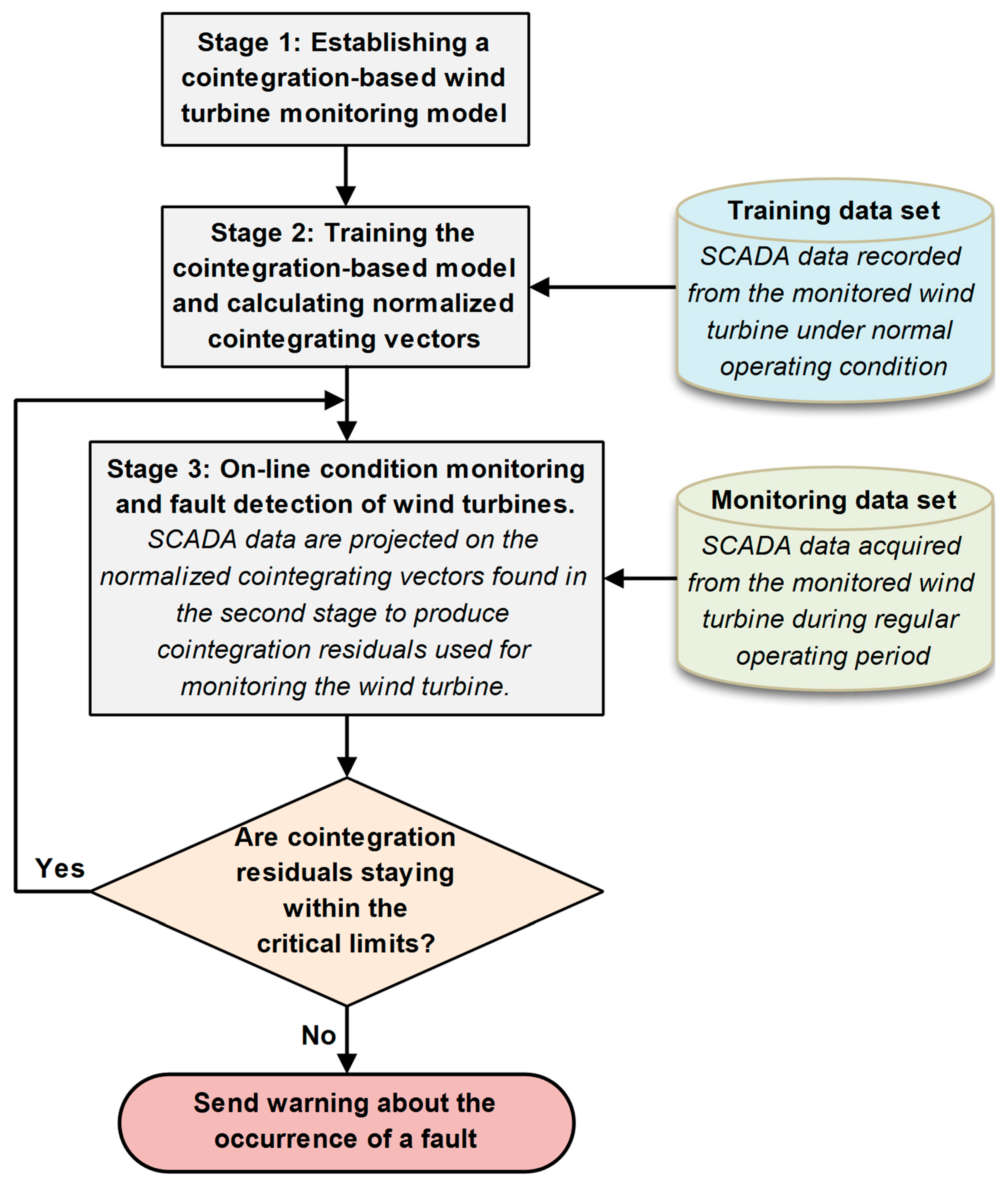
In the present work, the cointegration technique has been exploited for on-line condition monitoring and fault detection of wind turbines using SCADA data. The entire cointegration-based computation procedure, consisting of three stages, is shown in Figure 1. In the following, these stages are described and discussed.
3.1. Establishing a Cointegration-Based Wind Turbine Monitoring Model
The purpose of the first stage is to establish a cointegration model for a given wind turbine. Specifically, a number of key process parameters of the wind turbine are required to be selected to form the model. A cointegration model is described by Equation (4), where variables represent the wind turbine parameters. In general, important operational parameters, such as the wind speed, generator speed, generated power, generator temperature, generator voltage, generator current, gearbox temperature, gearbox oil sump temperature, rotor bearing temperature, and rotor speed, can be chosen for this purpose. In this study, a cointegration model of the monitored wind turbine, formed with a set of process parameters, has the role of a wind turbine monitoring model. It is noted that at least two parameters must be selected such that a cointegration-based wind turbine monitoring model can be established.
The cointegration-based wind turbine monitoring model does not require all important operational parameters, as named above, to be included in the model. However, it is suggested that the wind speed and generated power should be employed in the cointegration-based monitoring model. The reason is because the relationship between wind speed and turbine power output represents the wind turbine power curve, which is one of the most important characteristics commonly used for wind turbine selection, capacity factor estimation, wind energy assessment and forecasting, and turbine performance and health monitoring [45]. In addition, temperature parameters of the generator and gearbox should be included in the model because a fault or an abnormal event, associated with the generator or gearbox component, is substantially a progressive phenomenon, that is, the initial sign of a gearbox or generator fault could appear several days or weeks before the fault event occurred in reality and it might be manifested by the increase in the gearbox bearing and/or generator temperature [28,31].
3.2. Training the Cointegration-Based Model and Calculating Normalized Cointegrating Vectors
In the second stage, the Johansen’s cointegration procedure [33] is deployed to train the cointegration-based monitoring model and calculate the normalized cointegrating vectors. The computation uses only SCADA data of several process parameters acquired from the monitored wind turbine under normal operating condition or a “healthy” state. In a simple description, the estimation of cointegrating vectors is executed in three steps. First is evaluating eigenvalues from the characteristic equation of a cointegration model. Next is sorting the eigenvalues from the largest to the smallest one. Then, the normalized cointegrating vectors are calculated from the sorted eigenvalues. Hence, the first and the last cointegrating vector are corresponding to the largest and the smallest eigenvalue, respectively. As reported in the previous works [19,34,35,41], the first cointegrating vector is said to create the most stationary cointegration residual. In other words, when projecting SCADA series stored in different process parameters on the first cointegrating vector, we obtain the first cointegration residual which is the most stationary combination of the cointegrated data. This cointegration residual has been considered as the best (or the most suitable) indicator used for fault and/or damage detection, as discussed in [19,34,35,36,40,41]. In this study, we also consider the first cointegration residual as the best feature and therefore use only this residual to monitor the health state of the wind turbine.
It is supposed that the training data set—selected for calculating the normalized cointegrating vectors—has a significant influence on the wind turbine health monitoring and fault detection results. As mentioned above, only the SCADA data recorded from a wind turbine operating in healthy condition should be used for this purpose. However, this requirement faces some challenges. First, model training and cointegrating vector calculation require sufficient amounts of normal operation data collected over a long period covering a representative range of wind turbine operating conditions. Certainly, when these data are scarce or when they are not representative for the turbine’s current normal operation state, fault detection may not feasible because the cointegration-based monitoring model cannot be trained properly. This is the case for newly installed wind turbines at the initial stage of their operation life when the amount of normal operation data accumulated is small, which cannot provide sufficient information for training cointegration-based models. Moreover, due to many unavoidable reasons, such as wind turbine ageing, subsystem replacements, software updates, or sensor recalibration, the normal operation data collected months or years before might be outdated and so they are no longer representative of the turbine’s current normal operation behaviour.
An alternative solution has been suggested by this work to deal with these challenges, that is, one may consider using several training data sets, which represent different normal operating modes of the wind turbine, to obtain different sets of normalized cointegrating vectors. Given that, more than one set of cointegration residuals can be employed to monitor the turbine and detect abnormal problems. This idea has been validated in this paper and the obtained results are presented in Section 5.
3.3. On-Line Condition Monitoring and Fault Detection of Wind Turbines
In the third stage, SCADA data—acquired from the monitored wind turbine during the regular operating period for producing electricity—are projected on the normalized cointegrating vectors found in the second stage to produce cointegration residuals used for monitoring the wind turbine. As explained in Section 2, this projection is simply equivalent to the multiplication of data vectors. Since SCADA data stored in each process parameter can be considered as a vector of time series, a cointegration residual (given by ) can be formed by multiplying vectors of SCADA series stored in different process parameters by one cointegrating vector. This implies that a cointegration residual also has the form of a sequence of time series. To obtain multiple cointegration residuals (denoted by ), one can multiply vectors of SCADA series stored in different process parameters by cointegrating vectors. This computation can be executed in a real-time manner on a computer-based monitoring system, which provides a simple on-line condition monitoring solution for wind turbines. As discussed in Section 3.2, only the first cointegration residual is used in this study to monitor the health condition of wind turbines. The creation of this residual is achieved by multiplying vectors of SCADA series, corresponding to the selected process parameters, by the first normalized cointegrating vector.
The possibility of using a cointegration-based monitoring model, in particular, the first cointegration residual, for on-line condition monitoring of wind turbines is explained here. When a new set of monitoring samples collected by the SCADA system are made available for analysis, these data are instantly projected on the first normalized cointegrating vector to create a new value of the first cointegration residual. This value is then compared with the critical limits, calculated as statistical confidence levels, of the control chart to determine whether the wind turbine is still operating under its normal condition. To present the monitoring process in an illustrative manner, the first cointegration residual is plotted against the critical region; if the residual crosses the upper or lower critical line, then it means that a fault would occur in the turbine.
4. Wind Turbine SCADA Data
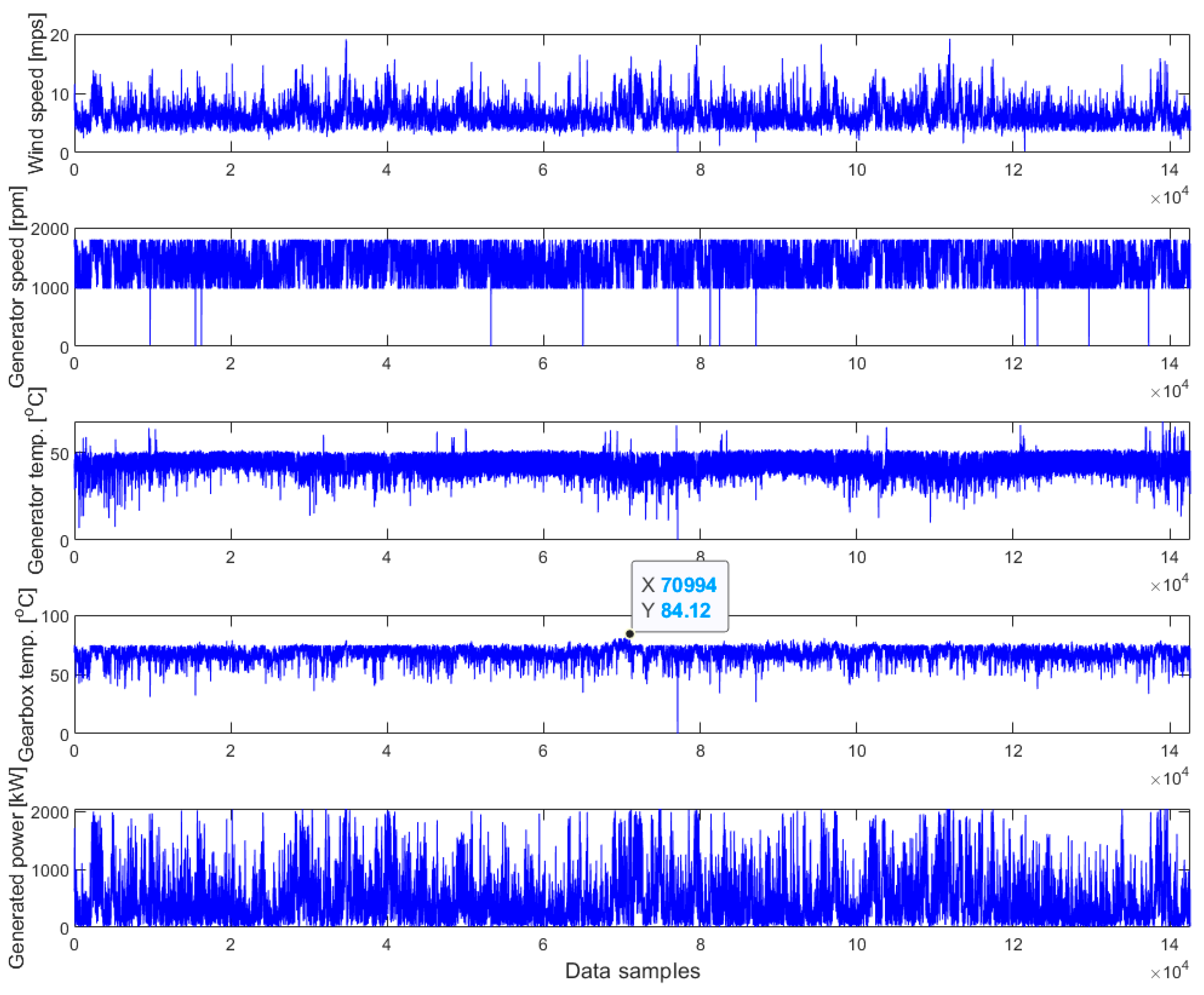
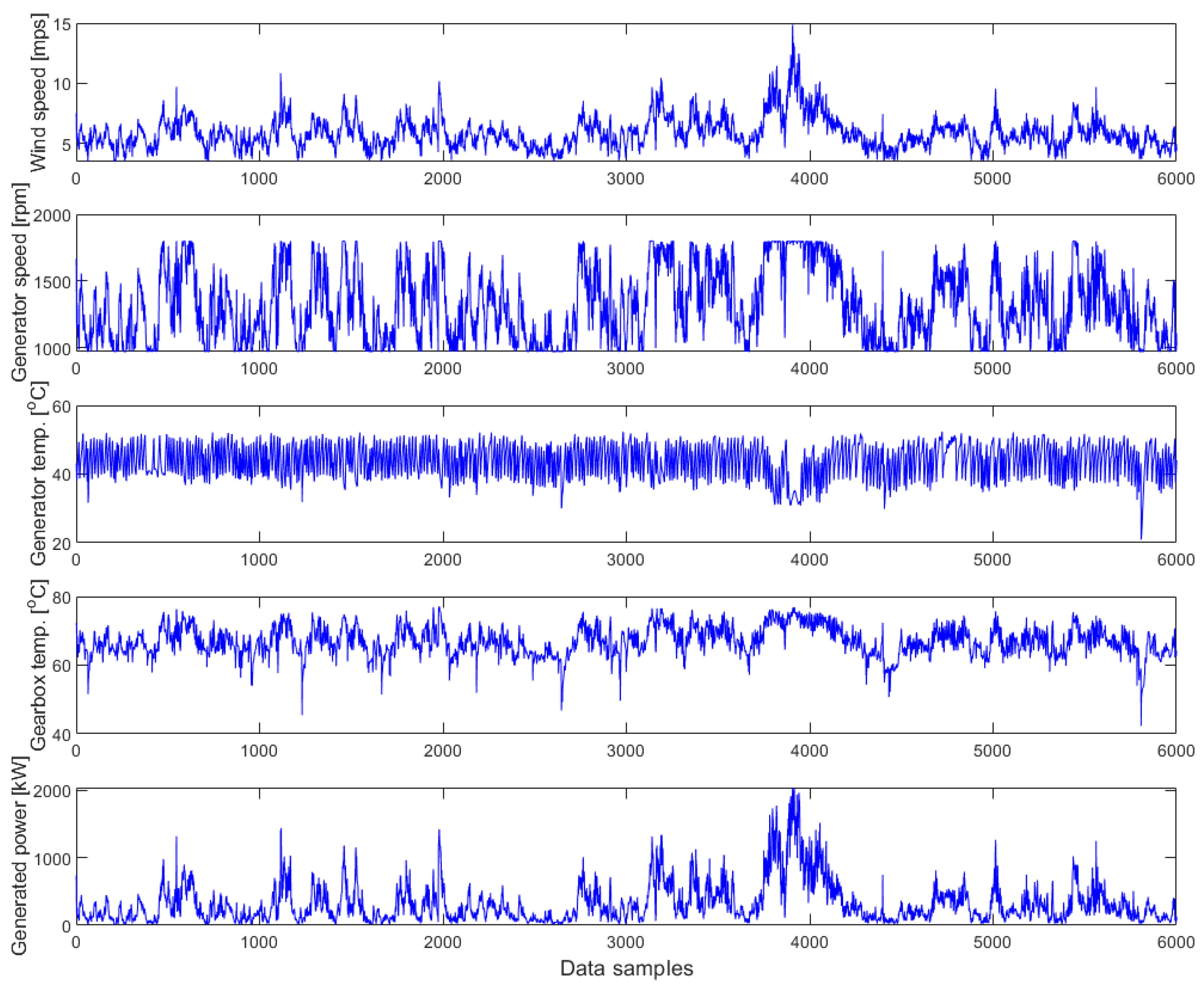
The long-term monitoring campaign of the La Houte Bourne onshore wind farm in Villeneuve-d’Ascq, France, over eight years (from 1 January 2013 to 31 December 2020) has provided for public a plentiful open-access SCADA data source [46]. The wind farm has four wind turbines of the MM82 model, manufactured by Senvion. The technical details of the wind turbines are given in Table 1. There were 34 process parameters measured at an interval of 10 min for each wind turbine and in total 1,057,868 samples were recorded. The data acquired for the wind turbine (labelled as R80721) over four years (from 1 January 2013 to 31 December 2016) were selected for the analysis in this study. There were 210,095 data samples recorded for each parameter. Before analysing the data using the cointegration-based method, data pre-processing and outlier cleaning procedures were performed to remove all samples associated with unphysical, corrupted, or missing values. As a result, we attained 142,613 data samples for each parameter. This four-year data collection of the wind turbine R80721 was recently used to validate a new wind turbine health monitoring method which is based on the Wilcoxon rank sum test [31]. SCADA data of this wind turbine, including the wind speed, generator speed, generator temperature, gearbox bearing temperature, and generated power, are plotted in Figure 2. These five process parameters are used in this study to create a cointegration-based monitoring model for the selected wind turbine. The validation results of the developed model are presented in the following section.
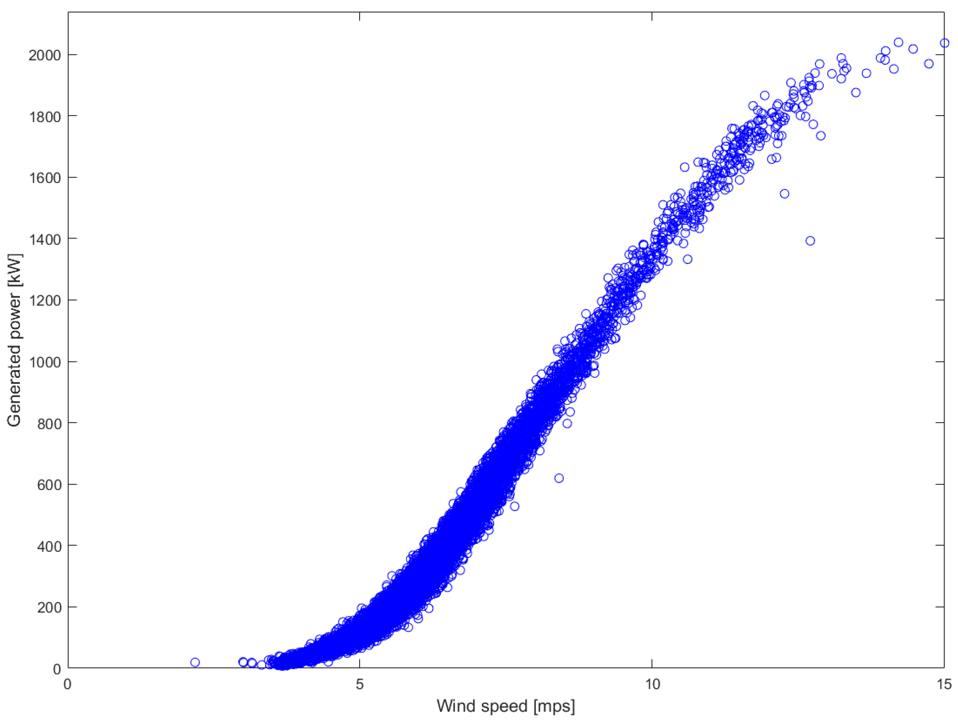
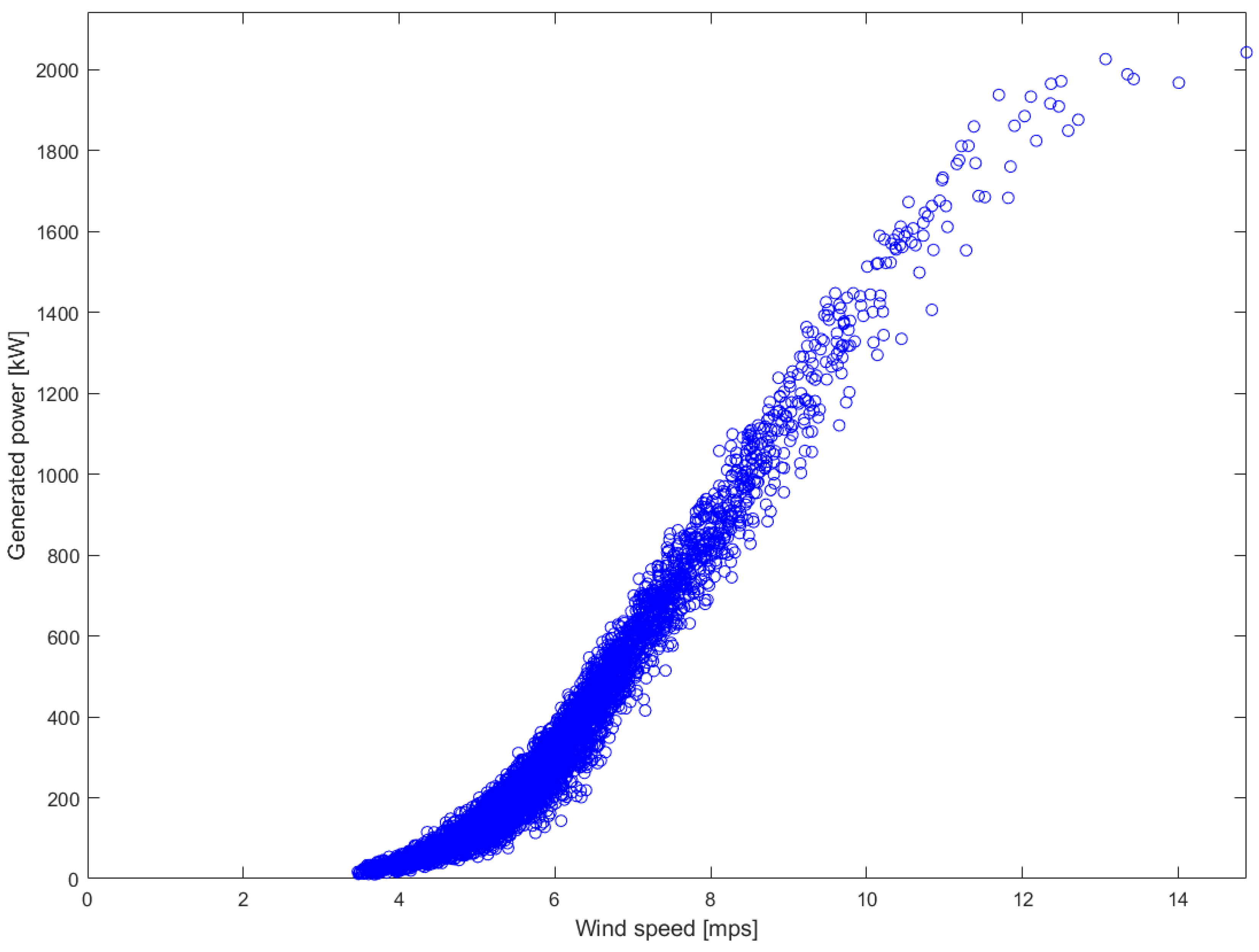
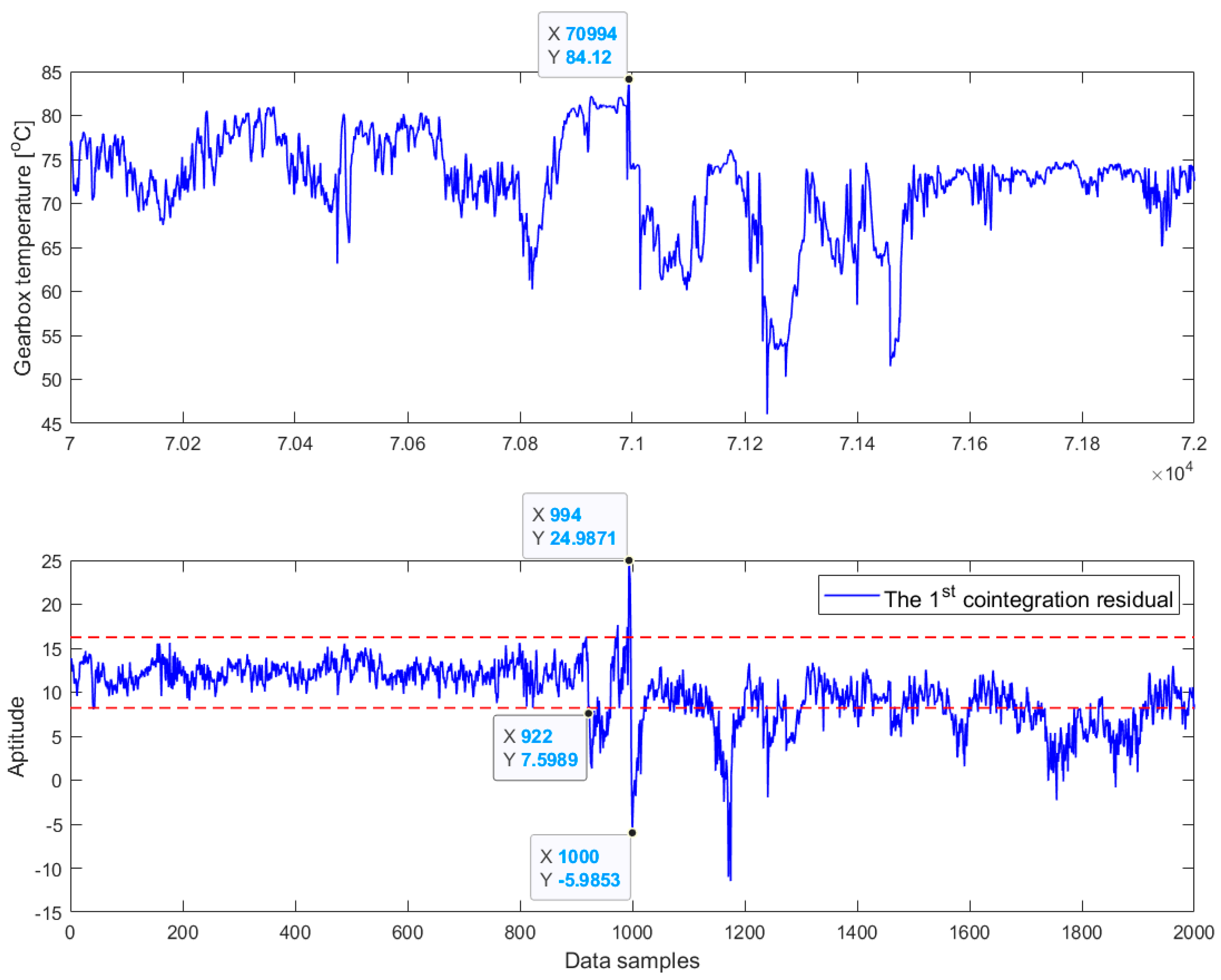
It is important to mention that during the four-year monitoring period of interest, the gearbox bearing temperature of the wind turbine R80721 was raised up to a peak value of 84.12 °C at the data sample 70,994, as marked in Figure 2. It is assumed that a fault in the gearbox is substantially a progressive phenomenon and that the initial signs of the anomaly, mostly indicated by a sudden increase in the gearbox bearing temperature, could appear at least several hours before its actual occurrence. Hence, it is crucial that this gearbox fault can be accurately predicted or detected early before the temperature of the gearbox bearing goes up. The wind turbine power curve, formed by plotting the generated power against the wind speed measured at the hub height for all data, is shown in Figure 3. The power curve describes how much electrical power output is produced by a wind turbine at different wind speeds.
5. Results and Discussion
This section presents the validation of the cointegration-based monitoring method, introduced in Section 3, using the wind turbine SCADA data, described in Section 4. A cointegration-based monitoring model for the wind turbine (R80721) was established using five process parameters, including the wind speed (), generator speed (), generator temperature (), gearbox temperature (), and generated power (), where are variables representing the wind turbine parameters. Two different sets of SCADA data were used to train the cointegration-based model and calculate the normalized cointegrating vectors. The first training data set involves 12,000 samples recorded before the occurrence of the gearbox fault (case 1), whereas the second one includes 6000 samples acquired after the fault occurrence (case 2). It is noted that these two training data sets represent the periods when the given wind turbine was operating in normal condition or healthy state. Cointegration residuals—obtained from projecting the testing data (2000 samples including the gearbox fault event) on the normalized cointegrating vectors—are used in control charts for operational condition monitoring and automated fault/abnormal detection.
5.1. Results Obtained by Using the First Training Data Set (Case 1)
The three-stage cointegration-based computation procedure (presented in Section 3) was deployed for the case study. Following Equation (4), we first established a cointegration-based monitoring model for the wind turbine (R80721). This model has the form
In the next stage, the cointegration-based wind turbine monitoring model was trained, and then the normalized cointegrating vectors were estimated using the Johansen’s cointegration method [33]. SCADA data within the sample points [17,000–29,000], corresponding to 12,000 samples recorded before the gearbox fault occurrence, were used for this purpose. These data are plotted in Figure 4 for the five process parameters. The wind turbine power curve in this case is shown in Figure 5. The minimum and maximum values of each process parameter used for training the cointegrating vectors are provided in Table 2. As a result, we obtained four normalized cointegrating vectors (in the form of four column vectors), which are given as follows:
where the first normalized cointegrating vector is specified by the first column, the second cointegrating vector is specified by the second column, and so on.
It is noted that in this case the constant vector , where , is found as . As mentioned in Section 3.2, only the first cointegration residual is used in this study to monitor the health condition of wind turbines. This cointegration residual is created by multiplying five vectors of the SCADA series (i.e., testing data), corresponding to the five selected process parameters, by the first normalized cointegrating vector. Therefore, the first cointegration residual () can be written as
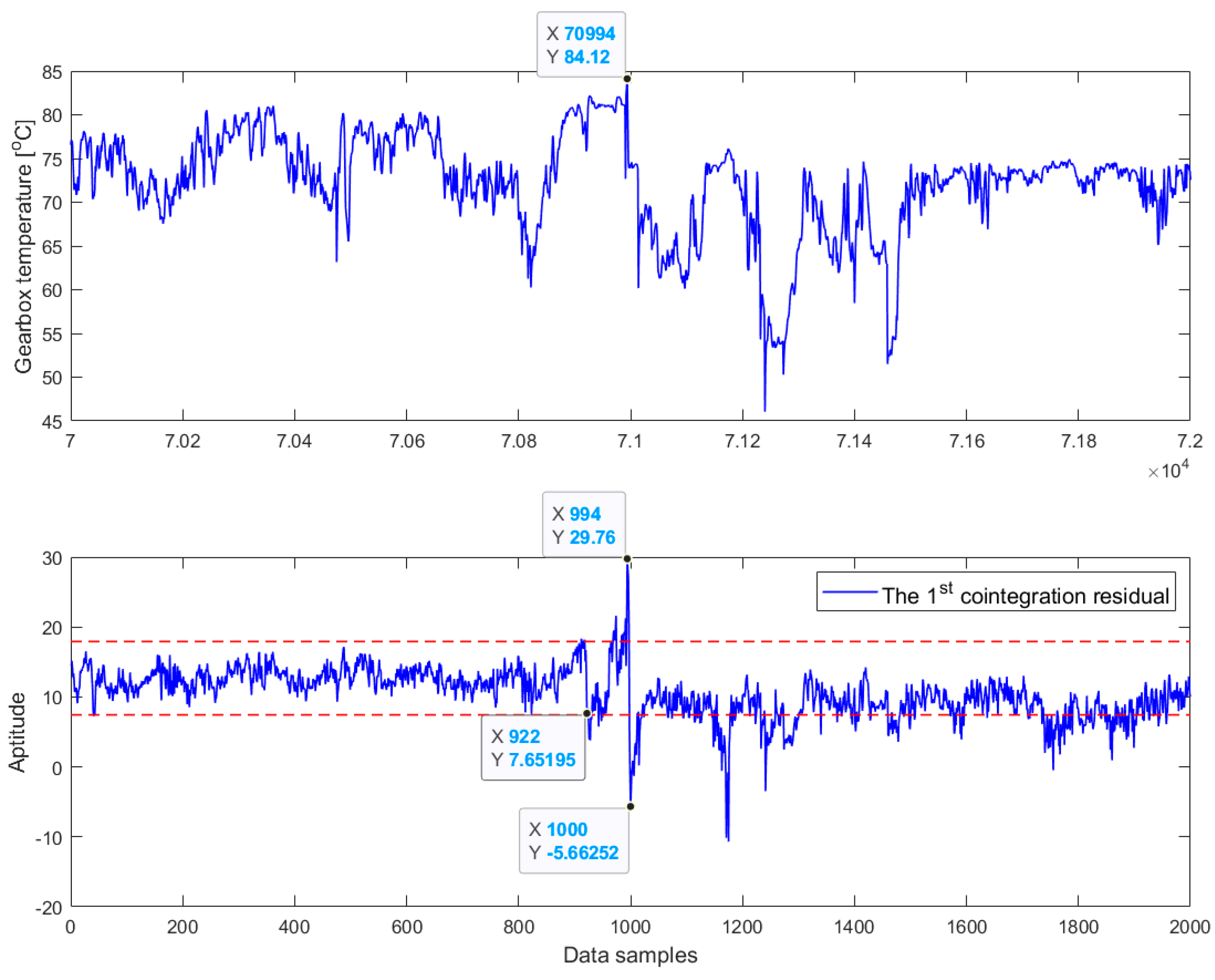
As mentioned in Section 4, the abnormal temperature and fault in the gearbox bearing occurred at the data sample 70,994. Hence, we selected 2000 data samples consisting of the sample points from 70,000 to 72,000, i.e., covering the gearbox fault event, as the testing data for each process parameter. Next, 2000 data samples of five process parameters are inserted into variables in Equation (8). This creates the first cointegration residual in the form of a time series with 2000 samples. The obtained cointegration residual is plotted together with the gearbox temperature in Figure 6 for the comparison. In addition, the residual is plotted against the 99.9% statistical confidence intervals. The confidence interval—with respect to the average of the residual—was calculated as , where and are the mean and standard deviation. The first 900 sample points of the residual were used for calculating the confidence interval. The two red dotted horizontal lines specify the critical limits of the confidence interval. During the monitoring, if the cointegration residual stays within these two lines, this means that the monitored wind turbine is operating in the healthy state. On the contrary, a fault would appear whenever the residual goes beyond the confidence levels. We can observe that the gearbox fault could be detected at data sample 922 in the residual timescale (or 70,922 in the SCADA data timescale). This implies that the anomaly was detected about 720 min (or 12 h) before its actual occurrence at the data sample 70,994.
5.2. Results Obtained by Using the Second Training Data Set (Case 2)
The computation procedure in Section 3 was applied for this case study. Regarding the first stage, we used the same cointegration-based monitoring model for the wind turbine (R80721), which was previously established for case 1 and given by Equation (7). However, in the second stage the cointegration-based wind turbine monitoring model was trained and then the normalized cointegrating vectors were estimated using SCADA data within the sample points [130,000–136,000], corresponding to 6000 samples recorded after the occurrence of the gearbox fault. These data are plotted in Figure 7 for the five process parameters. The wind turbine power curve in this case is shown in Figure 8. The minimum and maximum values of process parameters used for training the cointegrating vectors are given in Table 3. As a result, we obtained four normalized cointegrating vectors (in the form of four column vectors), which are listed below:
The constant vector is equal to in this case. Again, the first cointegration residual is created by multiplying five vectors of the SCADA series (i.e., testing data), corresponding to the five selected process parameters, by the first normalized cointegrating vector. Therefore, the first cointegration residual () can be formed as
The same set of the testing data, i.e., 2000 data samples used for case 1 in Section 5.1, was also used in this case. After the testing data of five process parameters were inserted into variables in Equation (9), we obtained the first cointegration residual in the form of a time series with 2000 samples. The residual is also plotted together with the gearbox temperature in Figure 9 to illustrate the fault detection. The same confidence interval was applied in this case. Interestingly, the abnormal temperature in the gearbox bearing was detected at the same moment as reported in case 1, that is, at the data sample 922 in the residual timescale (or 70,922 in the SCADA data timescale). Therefore, the anomaly was detected about 720 min (or 12 h) before its actual occurrence at the data sample 70,994.
5.3. Discussion
The first important point to be discussed here is that for both cases investigated where different sets of SCADA data were used to estimate the cointegrating vectors, the first cointegration residuals obtained in Figure 6 (case 1) and Figure 9 (case 2) exhibit the same behaviour. To ease the observation and comparison, these two residuals are plotted together in Figure 10. We can observe that their amplitudes, shapes, and trends are almost identical. In particular, the moment of fault detection (at the data sample 922 in the residual timescale) and the peak (at the data sample 994) are the same in both cases. Interestingly, the peak is at the same moment as the fault occurrence.
Moreover, it is well known that a certain cointegration residual usually represents a long-run equilibrium relationship between the cointegrated time series [43]. In Figure 10, we can observe that for both cases the wind turbine exhibited a long-run equilibrium relationship until the moment (at the data sample 922) when the fault was detected. After passing the fault-related period, we can observe in both cases that the wind turbine established a new long-run equilibrium relationship approximately after data sample 1200.
6. Conclusions
This study has reported a new investigation on cointegration for wind turbine monitoring using a four-year SCADA data set acquired from a commercial wind turbine. We investigated for the first time what can be expected if two different sets of SCADA data, representing different normal operating modes of the given wind turbine, are used to train the cointegration-based monitoring model and calculate the normalized cointegrating vectors. The experimental results demonstrated that although different training data sets were used, the cointegration analysis created two residuals, having identical shapes and trends, which could detect the gearbox fault at the same moment. These findings have never been reported in the literature and would be helpful for the potential users of the method in the future.
In comparison with well-trained ML-based methods, the cointegration-based wind turbine monitoring solution may not provide very early warning signs about the fault occurrence. However, the simplicity of the proposed method is an essential factor in practical condition monitoring applications. Instead of analysing and interpreting many wind turbine parameters at the same time, by using this method, the wind turbine monitoring and fault detection process is as simple as observing the stability of a single cointegration residual in a control chart. This constitutes a simple and effective way to monitor the operating state and detect incipient failures of wind turbines in a wind farm. In addition, the use of multiple data sets to train the cointegration-based wind turbine monitoring model and calculate the normalized cointegrating vectors could improve the reliability of the condition monitoring and fault detection process.
In this study, the gearbox anomaly was detected about 12 h before its actual occurrence. However, it is expected in practice that the early fault detection should be at least some days or even weeks in advance for preventing wind turbine damages. Therefore, future study on adapting the cointegration-based monitoring method to make it possible for early fault prognosis in wind turbines has been planned. In addition, the training data sets were analysed without cleaning so that the wind turbine power curves contained a lot of outliers. The early fault detection would have improved if we had performed the power curve cleaning.
This study presents some promising results. However, some works can be suggested for the further development and validation of the method. First, the cointegration-based monitoring method should be validated using other SCADA data sets which involve different fault types associated with main turbine components. Second, it would be interesting to investigate if the normalized cointegrating vectors calculated for a wind turbine with sufficient training data can be reused for other wind turbines with scarce or limited operation data, especially for newly installed wind turbines. In other words, this future work will involve the transfer learning of cointegration-based normal behaviour models between wind turbines.
Funding
This research received no external funding.
Data Availability Statement
No new data were created in this study. The wind turbine SCADA data sets used in this study are mentioned in the Acknowledgments; the access to these data sets is given in Ref. [46].
Acknowledgments
The author would like to thank the ENGIE company for opening up and sharing SCADA data of the La Houte Borne wind farm.
Conflicts of Interest
The author declares no conflict of interest.
References
- Global Wind Energy Council. Global Wind Report: Annual Market Update 2022. Published in April 2022. Available online: https://gwec.net/global-wind-report-2022/ (accessed on 10 September 2022).
- Polish Wind Energy Association (PSEW); DWF Group; TPA Poland/Baker Tilly TPA. Onshore Wind Energy in Poland Annual Report; PSEW: Serock, Poland; DWF Group: Manchester, UK; TPA Poland/Baker Tilly TPA: Warsaw, Poland, 2021. [Google Scholar]
- Kusiak, A.; Li, W. The prediction and diagnosis of wind turbine faults. Renew. Energy 2011, 36, 16–23. [Google Scholar] [CrossRef]
- Tchakoua, P.; Wamkeue, R.; Ouhrouche, M.; Slaoui-Hasnaoui, F.; Tameghe, T.A.; Ekemb, G. Wind turbine condition monitoring: State-of-the-art review, new trends, and future challenges. Energies 2014, 7, 2595–2630. [Google Scholar] [CrossRef] [Green Version]
- Tautz-Weinert, J.; Watson, S.J. Using SCADA data for wind turbine condition monitoring—A review. IET Renew. Power Gener. 2017, 11, 382–394. [Google Scholar] [CrossRef] [Green Version]
- Salameh, J.P.; Cauet, S.; Etien, E.; Sakout, A.; Rambault, L. Gearbox condition monitoring in wind turbines: A review. Mech. Syst. Signal Process. 2018, 111, 251–264. [Google Scholar] [CrossRef]
- Wang, T.; Han, Q.; Chu, F.; Feng, Z. Vibration based condition monitoring and fault diagnosis of wind turbine planetary gearbox: A review. Mech. Syst. Signal Process. 2019, 126, 662–685. [Google Scholar] [CrossRef]
- Zhu, J.; Yoon, J.M.; He, D.; Bechhoefer, E. Online particle-contaminated lubrication oil condition monitoring and remaining useful life prediction for wind turbines. Wind Energy 2015, 18, 1131–1149. [Google Scholar] [CrossRef]
- Pozo, F.; Vidal, Y.; Salgado, Ó. Wind Turbine Condition Monitoring Strategy through Multiway PCA and Multivariate Inference. Energies 2018, 11, 749. [Google Scholar] [CrossRef] [Green Version]
- Zhang, S.; Lang, Z.Q. SCADA-data-based wind turbine fault detection: A dynamic model sensor method. Control Eng. Pract. 2020, 102, 104546. [Google Scholar] [CrossRef]
- Jin, X.; Xu, Z.; Qiao, W. Condition monitoring of wind turbine generators using SCADA data analysis. IEEE Trans. Sustain. Energy 2021, 12, 202–210. [Google Scholar] [CrossRef]
- Stetco, A.; Dinmohammadi, F.; Zhao, X.; Robu, V.; Flynn, D.; Barnes, M.; Keane, J.; Nenadic, G. Machine learning methods for wind turbine condition monitoring: A review. Renew. Energy 2019, 133, 620–635. [Google Scholar] [CrossRef]
- Sun, S.; Wang, T.; Yang, H.; Chu, F. Condition monitoring of wind turbine blades based on self-supervised health representation learning: A conducive technique to effective and reliable utilization of wind energy. Appl. Energy 2022, 313, 118882. [Google Scholar] [CrossRef]
- Wang, A.; Pei, Y.; Qian, Z.; Zareipour, H.; Jing, B.; An, J. A two-stage anomaly decomposition scheme based on multi-variable correlation extraction for wind turbine fault detection and identification. Appl. Energy 2022, 321, 119373. [Google Scholar] [CrossRef]
- Zhang, Y.; Liu, W.; Wang, X.; Shaheer, M.A. A novel hierarchical hyper-parameter search algorithm based on greedy strategy for wind turbine fault diagnosis. Expert Syst. Appl. 2022, 202, 117473. [Google Scholar] [CrossRef]
- Xiang, L.; Yang, X.; Hu, A.; Su, H.; Wang, P. Condition monitoring and anomaly detection of wind turbine based on cascaded and bidirectional deep learning networks. Appl. Energy 2022, 305, 117925. [Google Scholar] [CrossRef]
- Schlechtingen, M.; Santos, I.F.; Achiche, S. Wind turbine condition monitoring based on SCADA data using normal behavior models. Part 1: System description. Appl. Soft Comput. 2013, 13, 259–270. [Google Scholar] [CrossRef]
- Yampikulsakul, N.; Byon, E.; Huang, S.; Sheng, S.; You, M. Condition monitoring of wind power system with nonparametric regression analysis. IEEE Trans. Energy Convers. 2014, 29, 288–299. [Google Scholar]
- Dao, P.B.; Staszewski, W.J.; Barszcz, T.; Uhl, T. Condition monitoring and fault detection in wind turbines based on cointegration analysis of SCADA data. Renew. Energy 2018, 116, 107–122. [Google Scholar] [CrossRef]
- Dao, P.B.; Staszewski, W.J.; Uhl, T. Operational condition monitoring of wind turbines using cointegration method. In Advances in Condition Monitoring of Machinery in Non-Stationary Operations, Applied Condition Monitoring; Timofiejczuk, A., Chaari, F., Zimroz, R., Bartelmus, W., Haddar, M., Eds.; Springer: Cham, Switzerland, 2018; Volume 9, Chapter 21; pp. 223–233. [Google Scholar]
- Dao, P.B. Condition monitoring of wind turbines based on cointegration analysis of gearbox and generator temperature data. Diagnostyka 2018, 19, 63–71. [Google Scholar] [CrossRef]
- Sun, X.; Xue, D.; Li, R.; Li, X.; Cui, L.; Zhang, X.; Wu, W. Research on condition monitoring of key components in wind turbine based on cointegration analysis. IOP Conf. Ser. Mater. Sci. Eng. 2019, 575, 012015. [Google Scholar] [CrossRef]
- Zhang, B.; Zhang, C.; Duan, H.; Ma, Y.; Li, J.; Cui, L. Realization of condition monitoring of gear box of wind turbine based on cointegration analysis. In Advances in Asset Management and Condition Monitoring. Smart Innovation, Systems and Technologies; Ball, A., Gelman, L., Rao, B., Eds.; Springer: Cham, Switzerland, 2020; Volume 166, pp. 281–291. [Google Scholar]
- Qadri, B.A.; Ulriksen, M.D.; Damkilde, L.; Tcherniak, D. Cointegration for detecting structural blade damage in an operating wind turbine: An experimental study. In Dynamics of Civil Structures, Conference Proceedings of the Society for Experimental Mechanics Series; Pakzad, S., Ed.; Springer: Cham, Switzerland, 2020; Volume 2, pp. 173–180. [Google Scholar]
- Xu, M.; Li, J.; Wang, S.; Yang, N.; Hao, H. Damage detection of wind turbine blades by Bayesian multivariate cointegration. Ocean Eng. 2022, 258, 111603. [Google Scholar] [CrossRef]
- Zhang, C.; Zhao, G.; Wu, Y. Wind Turbine Condition Monitoring Based on SCADA Data Co-integration Analysis. In Proceedings of IncoME-VI and TEPEN 2021. Mechanisms and Machine Science; Zhang, H., Feng, G., Wang, H., Gu, F., Sinha, J., Eds.; Springer: Cham, Switzerland, 2023; Volume 117, pp. 97–103. [Google Scholar]
- Letzgus, S. Change-point detection in wind turbine SCADA data for robust condition monitoring with normal behaviour models. Wind Energy Sci. 2020, 5, 1375–1397. [Google Scholar] [CrossRef]
- Dao, P.B. Condition monitoring and fault diagnosis of wind turbines based on structural break detection in SCADA data. Renew. Energy 2022, 185, 641–654. [Google Scholar] [CrossRef]
- Dao, P.B. A CUSUM-based approach for condition monitoring and fault diagnosis of wind turbines. Energies 2021, 14, 3236. [Google Scholar] [CrossRef]
- Latiffianti, E.; Sheng, S.; Ding, Y. Wind turbine gearbox failure detection through cumulative sum of multivariate time series data. Front. Energy Res. 2022, 10, 904622. [Google Scholar] [CrossRef]
- Dao, P.B. On Wilcoxon rank sum test for condition monitoring and fault detection of wind turbines. Appl. Energy 2022, 318, 119209. [Google Scholar] [CrossRef]
- Engle, R.F.; Granger, C.W.J. Cointegration and error-correction: Representation, estimation and testing. Econometrica 1987, 55, 251–276. [Google Scholar] [CrossRef]
- Johansen, S. Statistical analysis of cointegration vectors. J. Econ. Dyn. Control 1988, 12, 231–254. [Google Scholar] [CrossRef]
- Cross, E.J.; Worden, K.; Chen, Q. Cointegration: A novel approach for the removal of environmental trends in structural health monitoring data. Proc. R. Soc. A 2011, 467, 2712–2732. [Google Scholar] [CrossRef]
- Dao, P.B.; Staszewski, W.J. Cointegration approach for temperature effect compensation in Lamb wave based damage detection. Smart Mater. Struct. 2013, 22, 095002. [Google Scholar] [CrossRef]
- Dao, P.B.; Staszewski, W.J.; Klepka, A. Stationarity-based approach for the selection of lag length in cointegration analysis used for structural damage detection. Comput. Aided Civ. Infrastruct. Eng. 2017, 32, 138–153. [Google Scholar] [CrossRef]
- Coletta, G.; Miraglia, G.; Pecorelli, M.; Ceravolo, R.; Cross, E.J.; Surace, C.; Worden, K. Use of the cointegration strategies to remove environmental effects from data acquired on historical buildings. Eng. Struct. 2019, 183, 1014–1026. [Google Scholar] [CrossRef]
- Salvetti, M.; Sbarufatti, C.; Cross, E.J.; Corbetta, M.; Worden, K.; Giglio, M. On the performance of a cointegration-based approach for novelty detection in realistic fatigue crack growth scenarios. Mech. Syst. Signal Process. 2019, 123, 84–101. [Google Scholar] [CrossRef] [Green Version]
- He, H.; Wang, W.; Zhang, X. Frequency modification of continuous beam bridge based on co-integration analysis considering the effect of temperature and humidity. Struct. Health Monit. 2019, 18, 376–389. [Google Scholar] [CrossRef]
- Tomé, E.S.; Pimentel, M.; Figueiras, J. Damage detection under environmental and operational effects using cointegration analysis—Application to experimental data from a cable-stayed bridge. Mech. Syst. Signal Process. 2020, 135, 106386. [Google Scholar] [CrossRef]
- Turrisi, S.; Cigada, A.; Zappa, E. A cointegration-based approach for automatic anomalies detection in large-scale structures. Mech. Syst. Signal Process. 2022, 166, 108483. [Google Scholar] [CrossRef]
- Dao, P.B.; Staszewski, W.J. Cointegration and how it works for structural health monitoring. Measurement 2023, 209, 112503. [Google Scholar] [CrossRef]
- Zivot, E.; Wang, J. Modeling Financial Time Series with S-PLUS, 2nd ed.; Springer: New York, NY, USA, 2006. [Google Scholar]
- LeSage, J.P. Econometrics Toolbox. Available online: www.spatial-econometrics.com (accessed on 20 November 2022).
- Bilendo, F.; Meyer, A.; Badihi, H.; Lu, N.; Cambron, P.; Jiang, B. Applications and modeling techniques of wind turbine power curve for wind farms—A review. Energies 2023, 16, 180. [Google Scholar] [CrossRef]
- ENGIE OpenData, SCADA Datasets of La Houte Bourne Wind Farm. Available online: https://opendata-renewables.engie.com/explore/index (accessed on 16 August 2022).
Figure 1.
Flowchart of the cointegration-based computation procedure for wind turbine monitoring and fault detection.
Figure 1.
Flowchart of the cointegration-based computation procedure for wind turbine monitoring and fault detection.

Figure 2.
SCADA data plotted for the five wind turbine parameters used in this study to form a cointegration-based monitoring model.
Figure 2.
SCADA data plotted for the five wind turbine parameters used in this study to form a cointegration-based monitoring model.

Figure 3.
Wind turbine power curve.

Figure 4.
Wind turbine SCADA data corresponding to the first training data set (case 1).

Figure 5.
Wind turbine power curve corresponding to the first training data set (case 1).

Figure 6.
Early detection of the abnormal temperature in the gearbox bearing by monitoring the first cointegration residual.
Figure 6.
Early detection of the abnormal temperature in the gearbox bearing by monitoring the first cointegration residual.

Figure 7.
Wind turbine SCADA data corresponding to the second training data set (case 2).

Figure 8.
Wind turbine power curve corresponding to the second training data set (case 2).

Figure 9.
Early detection of the abnormal temperature in the gearbox bearing by monitoring the first cointegration residual.
Figure 9.
Early detection of the abnormal temperature in the gearbox bearing by monitoring the first cointegration residual.

Figure 10.
Comparison of the first cointegration residuals obtained from two cases: (top) case 1; (bottom) case 2.
Figure 10.
Comparison of the first cointegration residuals obtained from two cases: (top) case 1; (bottom) case 2.


Table 1.
Technical information of wind turbines in the wind farm.
| Technical Parameters | Value |
|---|---|
| Rated power | 2050 kW |
| Cut-in wind speed | 4 m/s |
| Cut-out wind speed | 22 m/s |
| Rated wind speed | 14.5 m/s |
| Operating temperature range | −20 °C to +35 °C |
| Rotor diameter | 82 m |
| Rotor area | 5281 m2 |
| Rotor blade length | 40 m |
| Hub height | 80 m |
Table 2.
Parameters used for training the cointegrating vectors (case 1) and their limited values.
| Parameters | Min Value | Max Value |
|---|---|---|
| Wind speed | 2.18 mps | 15.01 mps |
| Generator speed | 969.83 rpm | 1801.21 rpm |
| Generator temperature | 22.76 °C | 51.71 °C |
| Gearbox temperature | 42.04 °C | 78.85 °C |
| Generated power | 6.82 kW | 2038.92 kW |
Table 3.
Parameters used for training the cointegrating vectors (case 2) and their limited values.
| Parameters | Min Value | Max Value |
|---|---|---|
| Wind speed | 3.47 mps | 14.88 mps |
| Generator speed | 969.83 rpm | 1801.34 rpm |
| Generator temperature | 20.89 °C | 52.39 °C |
| Gearbox temperature | 42.32 °C | 77.09 °C |
| Generated power | 10.41 kW | 2042.91 kW |
Disclaimer/Publisher’s Note: The statements, opinions and data contained in all publications are solely those of the individual author(s) and contributor(s) and not of MDPI and/or the editor(s). MDPI and/or the editor(s) disclaim responsibility for any injury to people or property resulting from any ideas, methods, instructions or products referred to in the content. |
© 2023 by the author. Licensee MDPI, Basel, Switzerland. This article is an open access article distributed under the terms and conditions of the Creative Commons Attribution (CC BY) license (https://creativecommons.org/licenses/by/4.0/).
Share and Cite
MDPI and ACS Style
Dao, P.B. On Cointegration Analysis for Condition Monitoring and Fault Detection of Wind Turbines Using SCADA Data. Energies 2023, 16, 2352. https://doi.org/10.3390/en16052352
AMA Style
Dao PB. On Cointegration Analysis for Condition Monitoring and Fault Detection of Wind Turbines Using SCADA Data. Energies. 2023; 16(5):2352. https://doi.org/10.3390/en16052352
Chicago/Turabian StyleDao, Phong B. 2023. "On Cointegration Analysis for Condition Monitoring and Fault Detection of Wind Turbines Using SCADA Data" Energies 16, no. 5: 2352. https://doi.org/10.3390/en16052352
Note that from the first issue of 2016, this journal uses article numbers instead of page numbers. See further details here.