

Assessment of Energy Consumption Characteristics of Ultra-Heavy-Duty Vehicles under Real Driving Conditions

1
School of Mechanical Engineering, Chonnam National University, 77 Yongbong-ro, Buk-gu, Gwangju 61186, Republic of Korea
2
National Institute of Environmental Research, 42 Hwangyeong-ro, Seo-gu, Inchon 22689, Republic of Korea
3
School of Mechanical and Aerospace Engineering, Konkuk University, 120 Neungdong-ro, Gwangjin-gu, Seoul 05029, Republic of Korea
*
Author to whom correspondence should be addressed.
†
These authors contributed equally to this work.
Energies 2023, 16(5), 2333; https://doi.org/10.3390/en16052333
Submission received: 4 December 2022
/
Revised: 12 February 2023
/
Accepted: 22 February 2023
/
Published: 28 February 2023
(This article belongs to the Topic Energy Saving and Energy Efficiency Technologies)
Abstract
:Passenger cars account for the largest share of GHG emissions in the road sector. However, given that the number of heavy-duty vehicles registered is lower but accounts for about a quarter of GHG emissions in the road sector, it is necessary to reduce carbon dioxide (CO2) emissions by improving the fuel efficiency of heavy-duty vehicles. However, experiments using dynamometers during the vehicle development process consume a lot of time and cost. Conversely, simulations can quantitatively analyze the sensitivity of parameters and accelerate optimization. Therefore, in this study, we modeled a heavy-duty vehicle using an AVL Cruise simulation and analyzed the effects of payload, air drag coefficient, and rolling resistance on fuel economy, CO2 emission, and the valid window ratio among the moving average window (MAW) for three driving routes. When the average vehicle speed was higher, the effect of the air drag coefficient on fuel economy was high. Additionally, when the average vehicle speed was lowered, the effect of the reduced rolling resistance on improving fuel efficiency was higher than that of the reducing air drag. Thus, the fuel efficiency improvement rate according to each 10% decrease in rolling resistance was higher by 2.2%, on average, in the low average speed route. Additionally, it was confirmed that the valid window ratio was high when driving in a section with a high vehicle speed first. Thus, the valid window ratio was almost 100% in the test of the route conditions starting from the highway section.
1. Introduction
Global warming is worsening due to the increased use of fossil fuels. Major countries around the world are setting goals to reduce greenhouse gas emissions to solve the global warming problem and drawing up specific plans to realize these goals. The European Commission has set a goal of reducing greenhouse gas emissions for the transportation sector by 20% from 2008 to 2030 and by 60% from 1990 to 2050 [1]. A total of 14% of all greenhouse gases worldwide originate from the transportation sector [2]. Specially, 94.6% of the greenhouse gases from the transportation sector originate on roads, and heavy-duty vehicles account for 25.1% of greenhouse gas emissions in Europe [3]. Energy generated from fuel combustion in heavy-duty vehicles is lost to air resistance (13.4%), rolling resistance (13.2%), and other mechanisms (6%) [4]. Therefore, a reduction in air resistance, the rolling resistance of tires, and idling are required to improve the fuel efficiency of vehicles.
Heavy-duty vehicles transporting heavy cargo require high torque in the low engine speed range for a stable start. In addition, heavy-duty vehicles require high fuel efficiency because their load is heavy. Diesel engines self-ignite combustion by directly injecting diesel fuel into the cylinder by making the combustion chamber in a high-temperature and high-pressure state, which can increase the engine stroke length and increase the compression ratio. This combustion method is difficult to effectively utilize under the high engine speed range but can increase inertial energy, torque, and thermal efficiency under the low engine speed range. Thus, heavy-duty vehicles mainly use diesel engines.
The number of registered cars in the Republic of Korea is increasing every year, and the number of registered diesel cars is also increasing. The proportion of diesel cars in the Republic of Korea is much higher than those in the U.S. and Japan. Although the proportion of registered heavy-duty vehicles among all vehicles is low (approximately 6.6%), the proportion of annual mileage, as of 2019, is approximately 26.4%, which is very high. In general, diesel engines have better fuel economy than gasoline engines. However, diesel fuel has a higher heating value and carbon dioxide emission coefficients than gasoline fuel, so the CO2 emissions per liter are higher. Thus, it is essential to reduce CO2 emissions by improving the fuel efficiency of heavy-duty vehicles because heavy-duty vehicles with low fuel efficiency account for about 25% of greenhouse gas emissions in the road sector.
Simulation methods are used for testing that reflect real road driving conditions while saving time and cost. Measurement methods, which utilize engine dynamometers, are mainly used to check the fuel efficiency and greenhouse gas emissions of heavy-duty vehicles accurately. However, this approach has the disadvantage of consuming a lot of time and cost. In addition, it cannot reflect the vehicle shape, weight, and transmission characteristics that affect greenhouse gas emissions. This, in turn, consumes a lot of time and cost. The method involving the use of a chassis dynamometer can reflect relatively more impact factors. However, the method still exhibits the disadvantage of using expensive equipment and consuming a lot of time. There are many different types of heavy-duty vehicles depending on the gross weight range, shaft structure, and purpose of use. In addition, various vehicle configurations are possible according to the trailer combination. Thus, a simulation method is used because it is difficult to measure greenhouse gas emissions using a chassis dynamometer for heavy-duty vehicles. Different simulation methods, such as the vehicle energy consumption calculation tool (VECTO) in Europe, greenhouse gas emissions model (GEM) in the United States, and Japanese fuel consumption model (JFCM) in Japan, have been used to regulate the fuel efficiency and greenhouse gases of heavy-duty vehicles. In Korea, it is also appropriate to use the simulation method because the distribution status of the chassis dynamometer for heavy-duty vehicles is significantly insufficient compared to that for light-duty vehicles. The use of vehicle simulation tools can reduce the cost of testing and optimize the vehicle during the design and development stages because comparative testing is possible in a short period of time. Furthermore, the fuel efficiency improvement technology, which is applicable in existing vehicles, can be evaluated with respect to various driving cycles and route conditions at no additional cost and is highly reproducible.
Recently, major countries, such as the U.S., those in Europe, and the Republic of Korea introduced real driving emission (RDE) regulations to measure pollutant emissions that reflect various variables on real roads, including intake conditions, road conditions, and driver characteristics. In the RDE regulations, data on greenhouse gas and emissions generated during real road driving can be measured via a portable emission measurement system (PEMS) [5,6,7]. Measurements using a PEMS can reflect factors that significantly impact fuel efficiency and the generation of emissions. Greenhouse gases are not regulated by the RDE test, but it is necessary to measure them using a real road driving test. In related previous studies, it was shown that the difference in CO2 emissions from laboratory conditions (measurement via engine- and chassis-dynamometers) and real driving conditions was approximately 42% on average in 1.1 million vehicles in eight countries [8]. In particular, the difference between laboratory and real road conditions is expected to be larger since heavy-duty vehicles are often overloaded on the real road, unlike the payload specified in the regulations. The difference in the chassis dynamometer test and real road driving emissions is the same for other pollutants and is the reason for the introduction of the RDE test. Thus, it is necessary to review the introduction of the RDE test for greenhouse gases, which has become important due to the recent carbon-neutral policy.
Su et al. [9] conducted an experiment on real road driving for three vehicle categories (M3, N2, and N3). For an ultra-heavy-duty vehicle, they evaluated the effects of the moving average window (MAW) method on the NOX result under two routes and three payload conditions. However, there was little difference in the driving section order and the fraction of the two routes. Currently, in Europe and Korea, the average emission per engine work for each segment is calculated in g/kWh using the MAW method. The size of the moving average window is defined as the period required to perform the same amount of work based on the work required for the worldwide harmonized transient cycle (WHTC) testing of the engine mounted on the test vehicle. After defining the initial moving average window, the window can be repeatedly defined and moved by the data acquisition cycle. Thus, the average value of emissions can be obtained from thousands of moving average windows. With respect to all moving average windows, a window with an average engine output exceeding 10% of the maximum engine output (as of 2021) is defined as a valid window. This should exceed 50% of the total number of moving average windows. Wang et al. [10] conducted an experiment on real road driving for three light-duty vehicles. They analyzed the effect of altitude on CO2 emissions and the MAW boundary condition. For a naturally aspirated vehicle, they reported that the higher the altitude, the lower the CO2 emission. However, it was difficult to confirm the effect of the test route characteristics because the other differences were unknown except for the altitude of the test route. Even more, it is important to understand the influence of the route and driving characteristics because the emission result varies in accordance with the order and fraction of the driving section owing to the characteristics of the MAW calculation. Previous studies on vehicle simulation are as follows: Katreddi et al. [11] predicted a heavy-duty truck’s total and instantaneous fuel consumption on a trip based on very few key parameters such as engine load, engine speed, and vehicle speed using an artificial neural network (ANN) model. However, fuel consumption prediction regression models, in which altitude data are not input, show poor prediction accuracy under different route conditions. In addition, Zeng et al. [12] predicted a light-duty vehicle’s real-world fuel consumption rate based on the records reported by the private vehicle using five artificial intelligence regression models. They reported that vehicle manufacturers or brands were also major factors influencing fuel consumption projections. Thus, it is appropriate to use a vehicle dynamics-based simulation method to analyze the effect of route conditions on fuel consumption. Fontaras et al. [13] used VECTO, a European vehicle simulation tool, to predict instantaneous and cumulative fuel consumption and compared the results from VECTO with predictions from other simulation tools, including Cruise (AVL), Autonomie (Argonne National Laboratory), and passenger car and heavy-duty emission models (PHEM and TUG). The comparisons confirmed that VECTO’s prediction error rate was within 4% and was similar to that of other simulation tools. Srinivasan and Kothalikar [14] quantitatively analyzed the effects of driving resistance factors such as rolling resistance, aerodynamic drag, and climbing (gradient) resistance on fuel economy and CO2 emissions in heavy-duty vehicles using AVL Cruise. Furthermore, Ko and Choi [15] calculated the fuel-cut inertial driving effect in accordance with the slope and deceleration of the downhill section using AVL Cruise and confirmed that an increase in the downhill gradient can lead to a decrease in the deceleration, which, in turn, increases fuel efficiency.
Although standards for the section order, average vehicle velocity, and driving time are regulated in each country, there may be differences in acceleration/deceleration rates and altitude characteristics depending on routes and traffic conditions. Although the aforementioned previous studies analyzed the effects of various factors on fuel efficiency, there are insufficient studies analyzing fuel efficiency characteristics according to various route characteristics for the same vehicle. In addition, as mentioned above, if the regulations to measure greenhouse gas under real road driving conditions are reviewed similar to other pollutants due to the carbon-neutral policy, it is necessary to study the success criteria and judgment of the RDE test. Specifically, RDE testing using a PEMS requires re-testing if the methods and criteria of the real road test are not satisfied. This requires additional time and significant additional costs. For the heavy-duty vehicles, if the vehicle’s load weight (payload) setting is not appropriate, then the test fails to satisfy the test criteria of the engine power. Furthermore, if after-treatment devices malfunction, then the test is considered as invalid, and this, in turn, will consume at least twice the time. For example, if a vehicle is tested with a minimum payload to prevent emissions under low-load or cold-start conditions that are not included in the valid window, then the engine power may be lowered. Hence, it may fail to satisfy the test success criteria and invalidate the test. In fact, the test failure can be overcome by extending the highway section. However, the time ratio for each section is regulated. In addition, EURO VII, which will be introduced in the future, will be designed to include the emission of the urban section in the valid window. Thus, it is expected that the extension of the highway section will be limited. Therefore, it is necessary to predict the criteria for generating minimal engine power in designing and controlling factors such as payload, tires, and frontal areas that affect greenhouse gas and improvements in emissions. In addition, RDE test routes vary by country and manufacturer, but research analyzed with the same vehicle for various routes is rare. Thus, this study also analyzed the effect of route characteristics on MAW. Although it is difficult to predict pollutants with 1D simulation tools, it is possible to predict if emission characteristics will change just by checking at changes in the MAW characteristics.
This study deals with the effect of the payload, air drag coefficient, and rolling resistance on fuel efficiency under three route conditions. In addition, it deals with whether the boundary conditions for the MAW are satisfied by predicting the engine power. We model a heavy-duty vehicle using AVL Cruise and apply driving data with three different driving characteristics to predict fuel consumption, engine power, and the ratio of the valid window. By quantitatively analyzing the effects of the aforementioned variables on the MAW boundary conditions as well as fuel efficiency, it is possible to consider which variables and driving conditions are sensitive to the test results. Thus, this study has a difference as it will assess which variables are effective in improving fuel efficiency while satisfying the MAW boundary condition under various route conditions.
2. Vehicle Modeling
2.1. Modeling of Test Vehicle
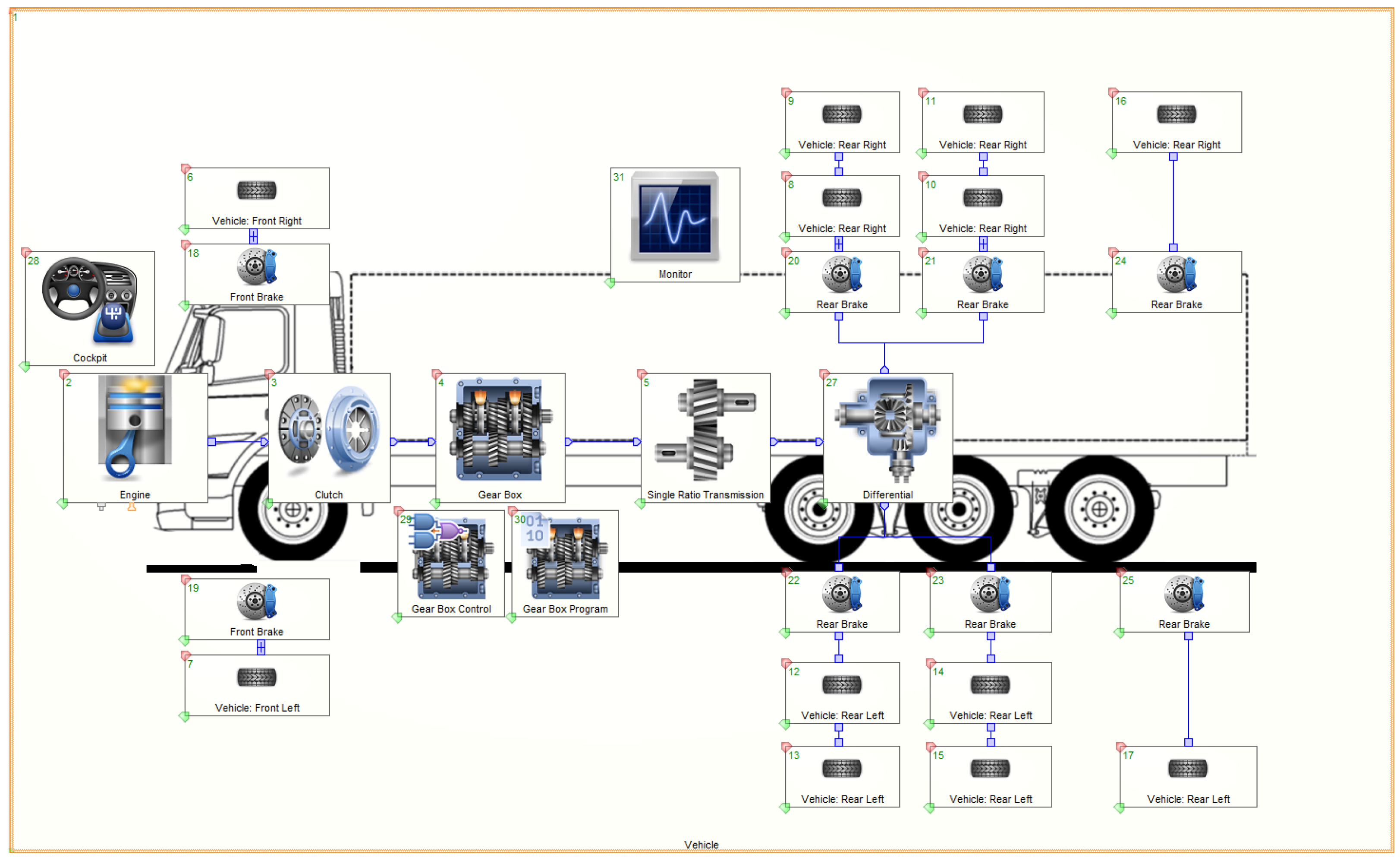
A test vehicle model created using AVL Cruise is shown in Figure 1. AVL Cruise is primarily a software for analyzing driving performance and fuel efficiency, and it exhibits the advantage of short computational time based on 1-D analysis. In this study, the backward calculation method was used to calculate the required engine operating range to drive with the input vehicle velocity profile, and the time step was 1 s. According to this method, the simulation time for the real test route of the modeling was about 10 s. The description and input data for the typical components are as follows:
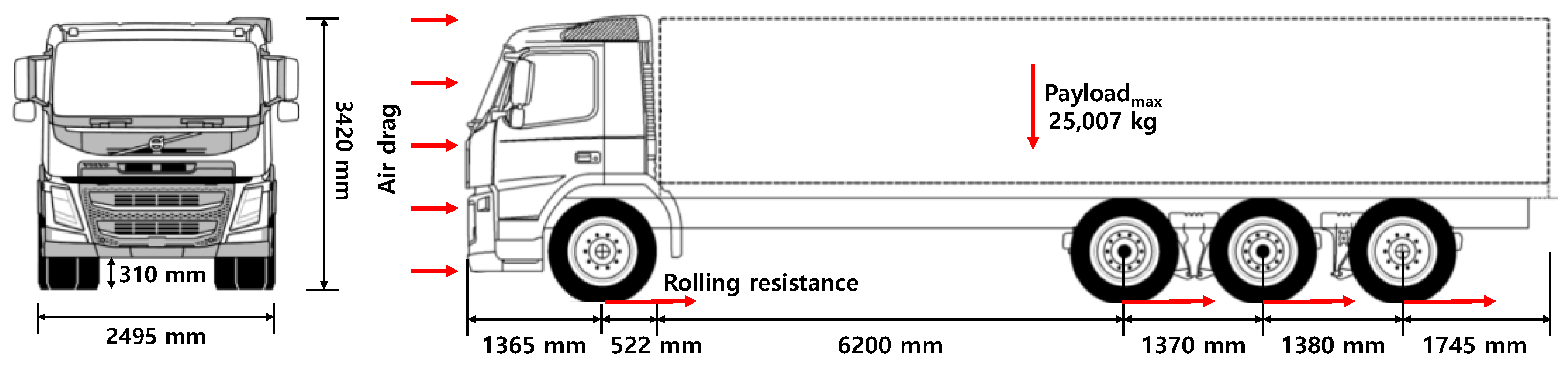
Data, such as vehicle dimensions, weight, center of gravity position, and air drag coefficient can be inputted in the ‘Vehicle’ component of the software. Based on these input values, resistance and wheel loads are calculated during driving. Specifically, the effects of acceleration, aerodynamic drag, and rolling resistance are considered. The modeled test vehicle consisted of an 8 × 4 type manualized automatic gearbox with a gross weight of 35 tonnes. Note that the 8 × 4 rigid truck is not a very typical truck. The dimensions of the vehicle are shown in Figure 2, and its detailed dimensions are listed in Table 1.
Furthermore, basic engine properties, such as fuel type, displacement volume, number of cylinders, and number of strokes are entered into the ‘Engine’ component. Additionally, the component models the engine in characteristic curves and map structures such as output and torque characteristics in accordance with engine speed and fuel economy map data. It also includes a temperature model to consider the effect of engine temperature on fuel consumption and emissions. The details of the engine are shown in Table 2.
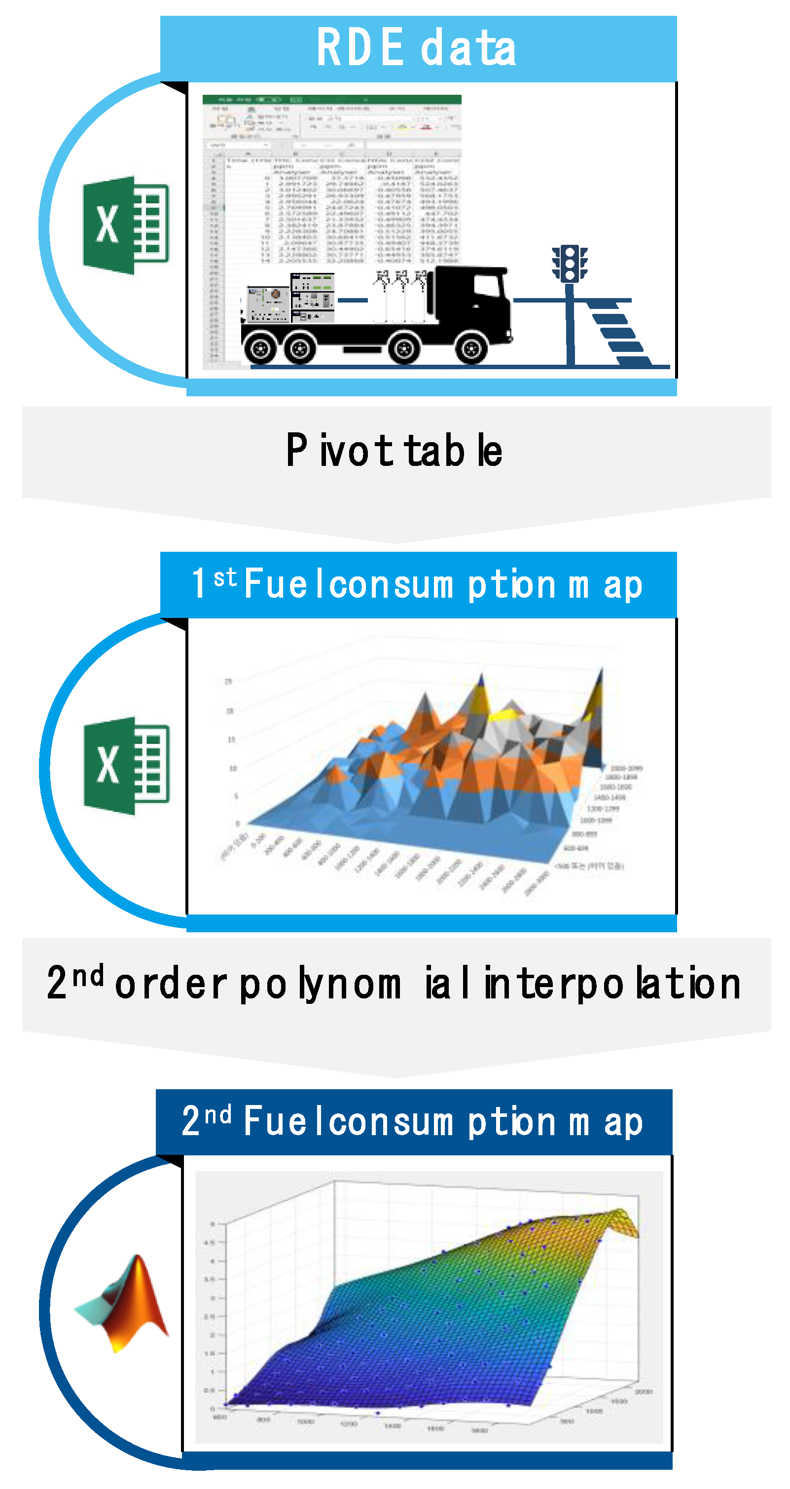
Fuel efficiency maps denote fuel consumption rates with respect to engine speed and torque, which, in turn, are parameters that are directly related to the calculated fuel economy [16]. In this study, fuel efficiency maps are derived from engine speed, torque, and fuel consumption data, which are measured over time while driving on real roads, and the sequence is shown in Figure 3. In the real road driving data, there is an operating range that is not measured, or only a small number of measurements are conducted in this operating range. Thus, the fuel efficiency map should be calibrated to derive fuel consumption data for these operating ranges. First, many operating points were divided into several operating ranges using the pivot table. The engine speed was set at 200 rpm intervals, and the engine torque was set at 100 Nm intervals, and the average fuel consumption rate (primary fuel efficiency map) of the operating range with the median value of these ranges was derived. Given that the primary fuel efficiency map is irregular in shape with a curved surface due to the unmeasured region, we performed a calibration task to smooth the curve by applying a quadratic polynomial interpolation method using MATLAB (secondary fuel efficiency map).
The shift ratio, mass inertia moment, and loss moment for all gear stages can be defined in the ‘Gear box’. In the case of manual gearboxes, they are shifted based on the defined gear stages along with the speed profile. For automatic gearboxes, the gearbox changes according to the shift point (defined as the engine speed and vehicle speed) were entered in the ‘Gear box control’, or the shift line was entered in the ‘gear box program’. Given that the real road driving data often do not measure gear stage, it should be calculated based on tire dimensions and transmission specifications. First, the wheel rotation speed (Swheel) is calculated by dividing the vehicle speed (V) by the tire circumference value (2RD) considered a dynamic rolling radius (RD), as shown in Equation (1), because the tire diameter changes when the vehicle is driven. The overall reduction gear ratio is then calculated, as shown in Equation (2), as the ratio of engine speed and wheel rotation speed. Furthermore, the gear ratio (transmission ratio) is calculated by dividing it into the final reduction ratio based on Equation (3). Finally, the gear stage that corresponds to this gear ratio is determined.
In Equations (1)–(3), SWheel and SEngine denote wheel rotation speed (1/min) and engine speed (1/min), respectively. Goverall and GFinal denote the overall reduction gear ratio and final reduction gear ratio, respectively. V and RD denote the velocity speed (m/s) and dynamic rolling radius (m), respectively. The ‘Wheel’ component allows the input of wheel diameters when the vehicle is stationary and driven and defines the rolling resistance with respect to the tire pressure, wheel load, ambient temperature, and vehicle speed. Rolling resistance can be calculated based on the wheel load, coefficient of rolling resistance, and wheel radius when driving. Longitudinal tire forces (circular force) can be calculated based on friction coefficients, wheel loads, and slip coefficients. If these factors are considered in different road conditions, then a variable friction coefficient can be defined according to the driving profile.
2.2. Driving Routes
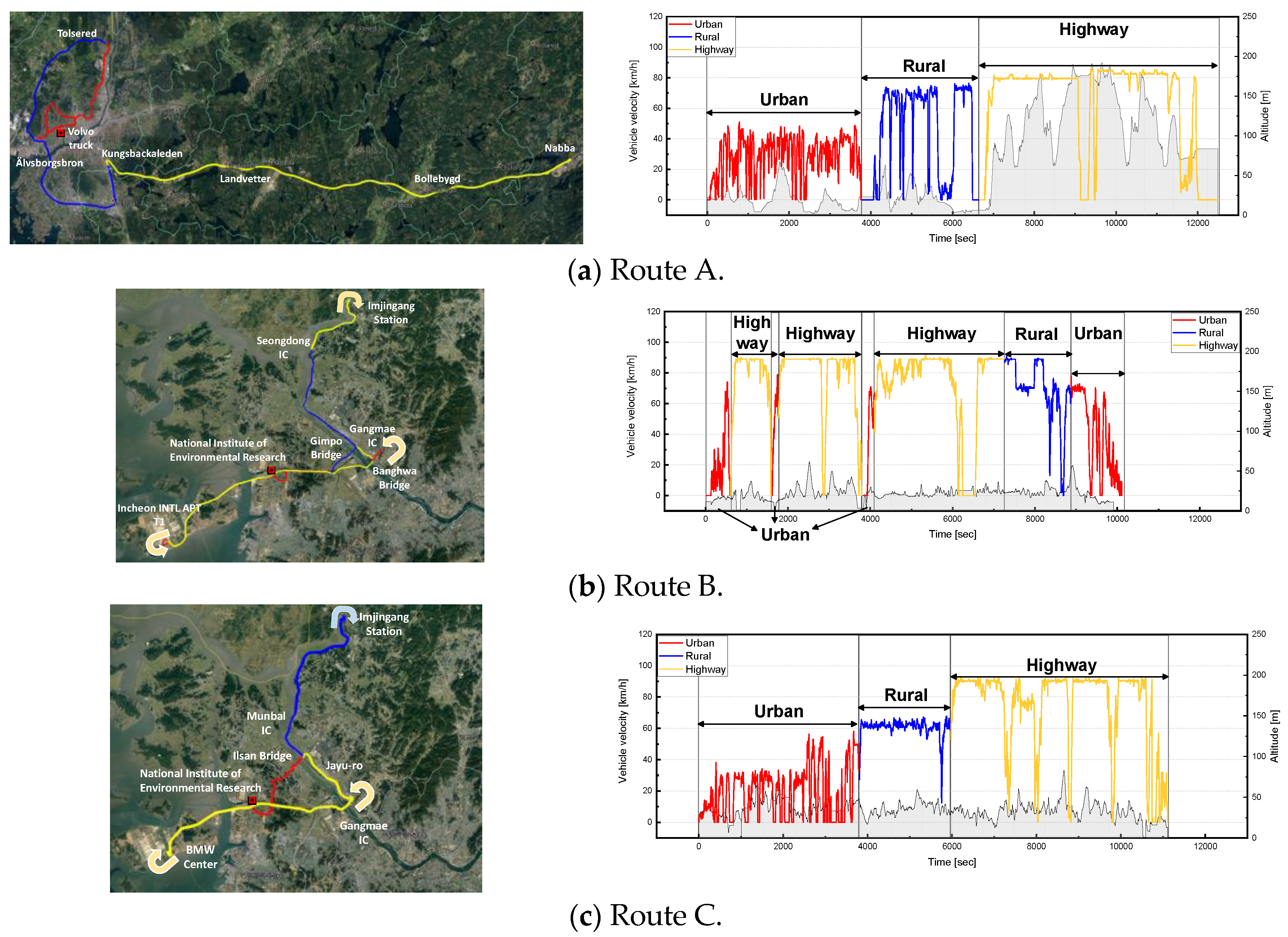
In this study, the effects of payload, rolling resistance, and air drag coefficient on fuel efficiency and CO2 emissions were analyzed for three different driving routes with different driving characteristics. The characteristics of the three driving routes are as follows: The velocity and the altitude profiles of each route with respect to time is shown in Figure 4. Table 3 lists the driving distance, driving time, and average vehicle velocity for each route.
Route A was used as the path when the test vehicle drives the RDE test, and the test vehicle was driven in the order of urban, rural, and highway sections. The total driven mileage of the test vehicle was 167 km, and the total driving time was 12,491 s. The average velocity on urban, rural, and highway sections was 28.6, 48.4, and 63.0 km/h, respectively. The altitude of Route A ranges from 0 to 20 m in the urban and rural sections. Then, entering the highway section, the altitude rises rapidly, and the vehicle drives in a wide range from 60 to 175 m. Route B was considered as a driving route for ultra-heavy-duty vehicles developed in the National Institute of Environmental Research (NIER). Unlike Route A, the cycle for Route B was in the order of highway, rural, and urban sections. The total driven mileage was 181 km, and the total driving time was 9913 s. The average velocity on urban, rural, and highway sections was 34.0, 70.2, and 75.9 km/h, respectively. In addition, the change in altitude during driving on Route B is the narrowest among the three routes. Route C was a modified version of Route B. In Route C, the driving cycle was in the order of urban, rural, and highway sections, unlike Route B. The total mileage driven on Route C was 163 km, and the total driving time was 11,112 s. The average velocity on urban, rural, and highway sections was 19.2, 60.6, and 74.4 km/h, respectively. Route C has a similar path to Route B. However, it has a wide altitude change during driving compared to Route B.
When comparing Route A and Route B, Route B exhibited a higher ratio of highway sections and higher average vehicle speed for all sections than Route A. When comparing Route A and Route C, the driving cycles for both routes were in the order of urban, rural, and highway. Furthermore, both routes exhibited a similar driving time ratio for each section. Additionally, the average vehicle velocity was approximately 10 km/h higher for Route C with the exception of the urban section. The comparison of Route B and Route C is similar to those of Route A and Route B because the driving characteristics of Route A and C are similar. Specifically, Route B had a large proportion of highway sections, and the average vehicle velocity for Route B was approximately 10 km/h higher in urban and rural sections, with similar highway sections.
3. Results and Discussion
3.1. Validation of Fuel Consumption Rate and Cumulative Fuel Consumption
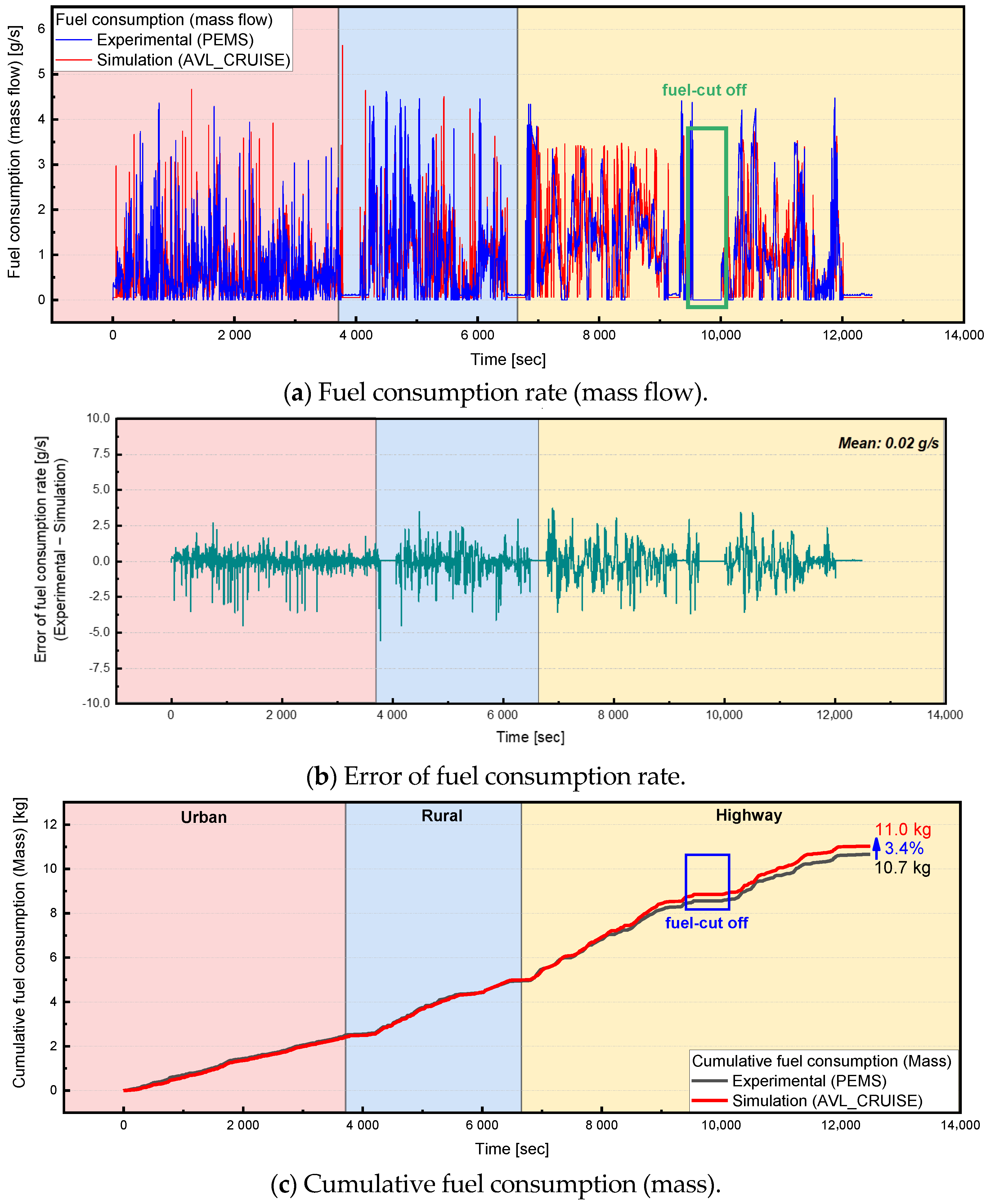
Figure 5 compares the predicted fuel consumption rate and cumulative fuel consumption in Route A with values measured by real road driving. A comparison of the fuel consumption rate in g/s with the test value indicates that the average error was 0.02 g/s. Compared to the experimental values, the cumulative fuel consumption in terms of mass (kg) exhibited an error of approximately 3.1% in urban areas, although the tendency was consistent. This is attributed to the large percentage of acceleration and deceleration in urban areas, and the accuracy of the shift was relatively low. Rural sections exhibited a low error of approximately 0.54% and displayed high predictive accuracy. For the highway section, the fuel-cut function was activated for the real road test [17]. However, cumulative fuel consumption was calculated to be about 3.1% higher than the experimental value. Consequently, the cumulative fuel consumption for the entire section was compared, and the error was estimated as 3.4%, which was sufficient to ensure the reliability of the results in the study.
3.2. Fuel Consumption Rate and Valid Window Ratio according to the Payload
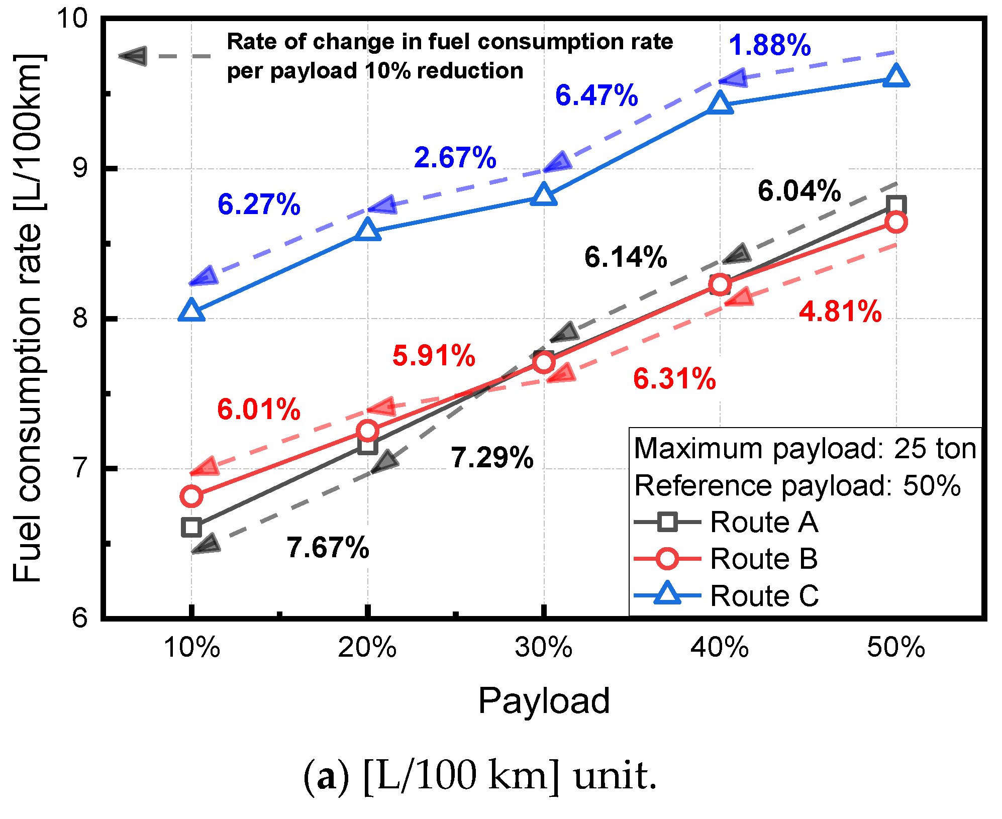
The maximum payload corresponds to the maximum weight that can be loaded within the range of the tonnage of cargo indicated on the truck, and the maximum payload of the test vehicle in the study was approximately 25 tonnes. Figure 6a shows the fuel consumption rate according to the payload for each driving route, where the unit of fuel consumption rate is one liter per 100 km [L/100 km]. The impact on the fuel consumption rate was analyzed as the payload during the real road test corresponded to 50% of the maximum payload and was reduced by 10% intervals based on the maximum payload. Overall, as the payload decreased, the fuel efficiency improved. As the payload decreased by 10% intervals from 50 to 10% based on the maximum payload, the fuel efficiency was improved by 6.79%, on average, in Route A. In the case of Route B and Route C, it was improved by 5.76 and 4.32%, on average, respectively. Thus, it can be confirmed that the fuel efficiency improvement rate in accordance with the payload varies depending on the route characteristics. Route A and Route B exhibited similar fuel consumption rates and can be seen to improve compared to Route C. In the case of Route A, the number of stops in urban and highway sections was less than that in Route C, and the vehicle was driven at a constant speed on highway sections. Thus, an improvement in the fuel consumption rate was observed. Additionally, in the case of Route B, an improvement in the fuel consumption rate was noted given the large proportion of highway sections and low variation in vehicle speed compared to Route C.
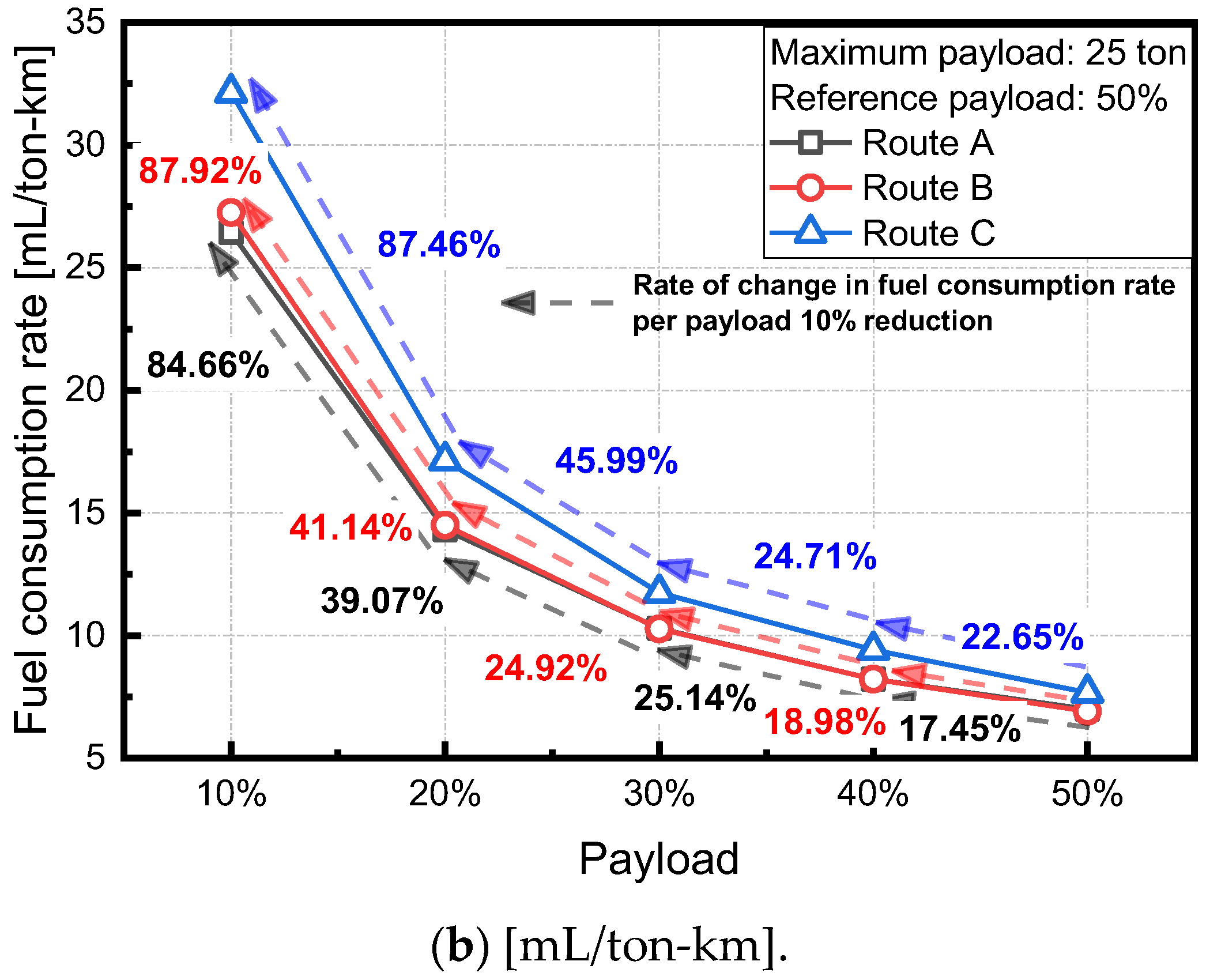
Figure 6b shows the conversion of the unit of Figure 6a to [mL/ton-km]. In Europe, CO2 is regulated as the average specific CO2 emission expressed in grams of CO2 per tonne-km [gCO2/t-km] for each manufacturer. Similarly, the United States adopts standard metrics in units of [gCO2/t-mile] or [gal/1000 t-mile] for vocational vehicles and combination tractors. This means the amount of fuel consumed to carry a tonne of cargo by a unit distance. In fact, it is necessary to analyze it as a unit considering cargo transport efficiency as transporting cargo once using heavy-duty vehicles is more advantageous in terms of oil costs and greenhouse gas emissions than transporting cargo several times with light-duty vehicles. As the payload decreased by 10% intervals from 50 to 10% based on the maximum payload, the fuel efficiency, considering cargo transport efficiency, deteriorated by 41.58, 43.24, and 45.20% on average under Routes A, B, and C, respectively. In addition, the gradient of fuel efficiency according to the reduction in the payload increased rapidly in the condition of a small payload range (payload 20%→10%). In summary, as the payload decreases, the fuel consumption rate of a heavy-duty vehicle is improved, but when considering the cargo transport efficiency, the amount of fuel required to transport a certain amount of cargo increases. For example, if the test vehicle carries 10 tonnes of cargo for 100 km, the fuel efficiency is 8.23 L/100 km (assuming Route A fuel efficiency), and the amount of fuel required is about 8.23 L. However, if the cargo is carried using by two vehicles loaded with 5 tonnes, fuel efficiency is improved to 7.15 L/100 km, but the total amount of fuel required increases to about 14.3 L.
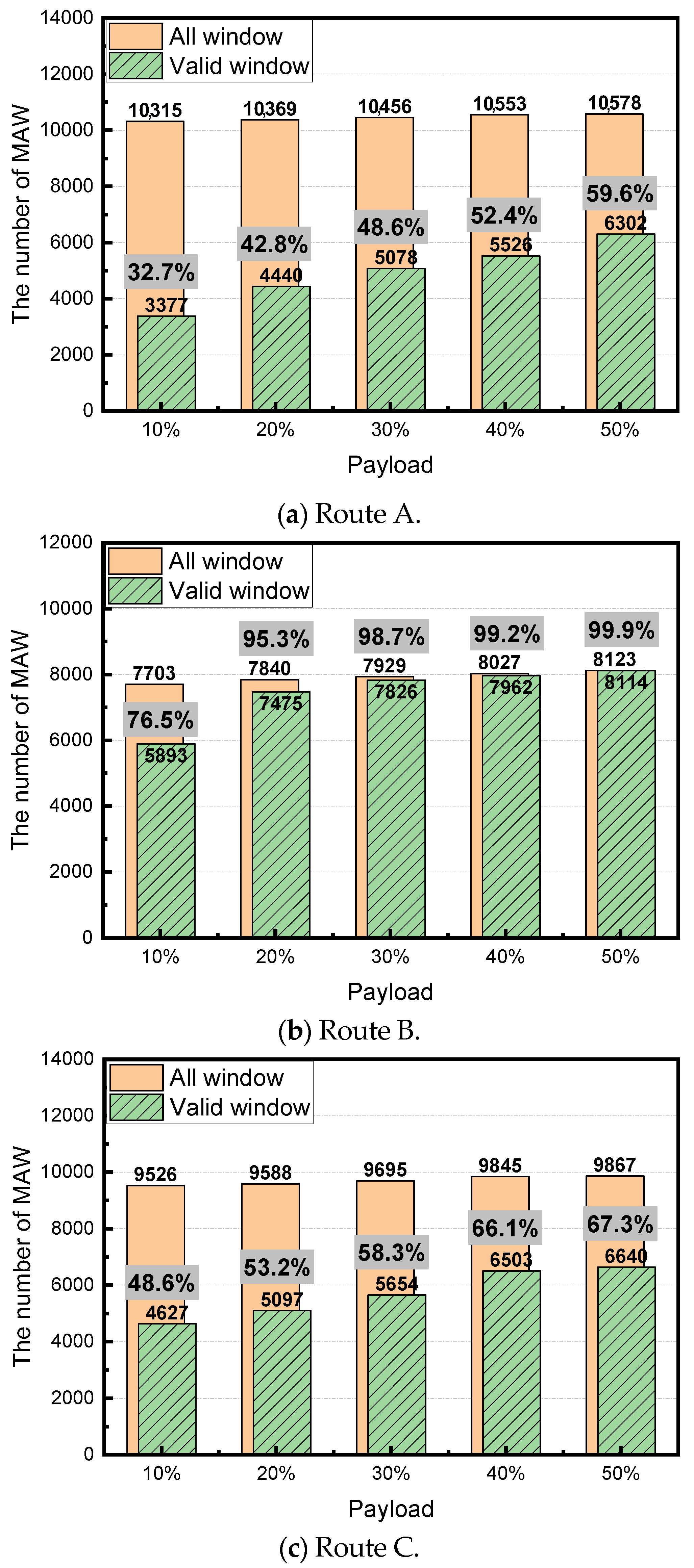
Figure 7 shows the number of MAWs according to the payload and ratio of the effective average window (valid window). The regulation at the time the test was conducted defines the valid window as a window with more than 20% of the maximum engine power. Thus, this study defined a valid window according to this regulation.
As shown in Figure 7, when the payload decreases on all routes, the number of moving average windows decreases, and the ratio of the valid window decreases. This is because the smaller the required output of the engine, the longer the time required to work as much as the reference work (WHTC work), and the larger size of the first MAW is defined. In addition, a large first MAW size means a small average power per segment, so the ratio of the valid window decreases. In the case of Route A, when the payload decreased by 30%, the ratio of the valid window was less than 50%, thereby indicating that the test was invalid. Route B with a high average vehicle speed and large proportion of highway sections exhibited a relatively small number of moving average windows given its relatively short test time. In addition, the ratio of the valid window was relatively high due to the high ratio of highway sections and higher mileage compared to those for shorter driving times. Additionally, it is judged that this will be affected by the highway section being driven first. When driving on the highway first, the engine power is high, so the size of the first MAW is small. This increases the number of MAWs but also increases the average power of small MAWs (per segment), increasing the ratio of the valid windows. In the case of Route C, the ratio of the valid window is almost the same as Route A because Route A is similar in the order of the driving section and section ratio. However, it was confirmed that the ratio of the valid window is 11.5% higher on average because Route C has a large change in the average speed and speed of the rural and highway sections. The boundary condition of the valid window is 50%. Hence, Routes A, B, and C can reduce the payload by 40, 10, and 20%, respectively, thereby improving fuel consumption by 6.4, 26.8, and 12%, respectively. This may result in an increase in average fuel efficiency by lowering the payload in the RDE test and may show a large difference from the real GHG emissions of heavy-duty vehicles. This is because the loading capacity of large vehicles on real roads is close to 100%. Therefore, it is necessary to review the revision of the valid window boundary condition. In addition, the rate of change of the valid window ratio according to the reduction in the payload was larger in Route A than in Route C. In other words, it shows that the effect of the payload on the valid window ratio is different depending on the route characteristics. The typical difference between the characteristics of Route A and Route C is the rate of change in altitude. In future, it is necessary to study the effect of the payload on the valid window ratio according to the altitude characteristics. If these findings are optimized and utilized for each vehicle, then it is expected that an appropriate payload setting can decrease time and cost via retesting. Additionally, the certification authority can determine whether the payload presented by the manufacturer is correct.
3.3. Fuel Consumption Rate and Valid Window Ratio according to the Air Drag Coefficient
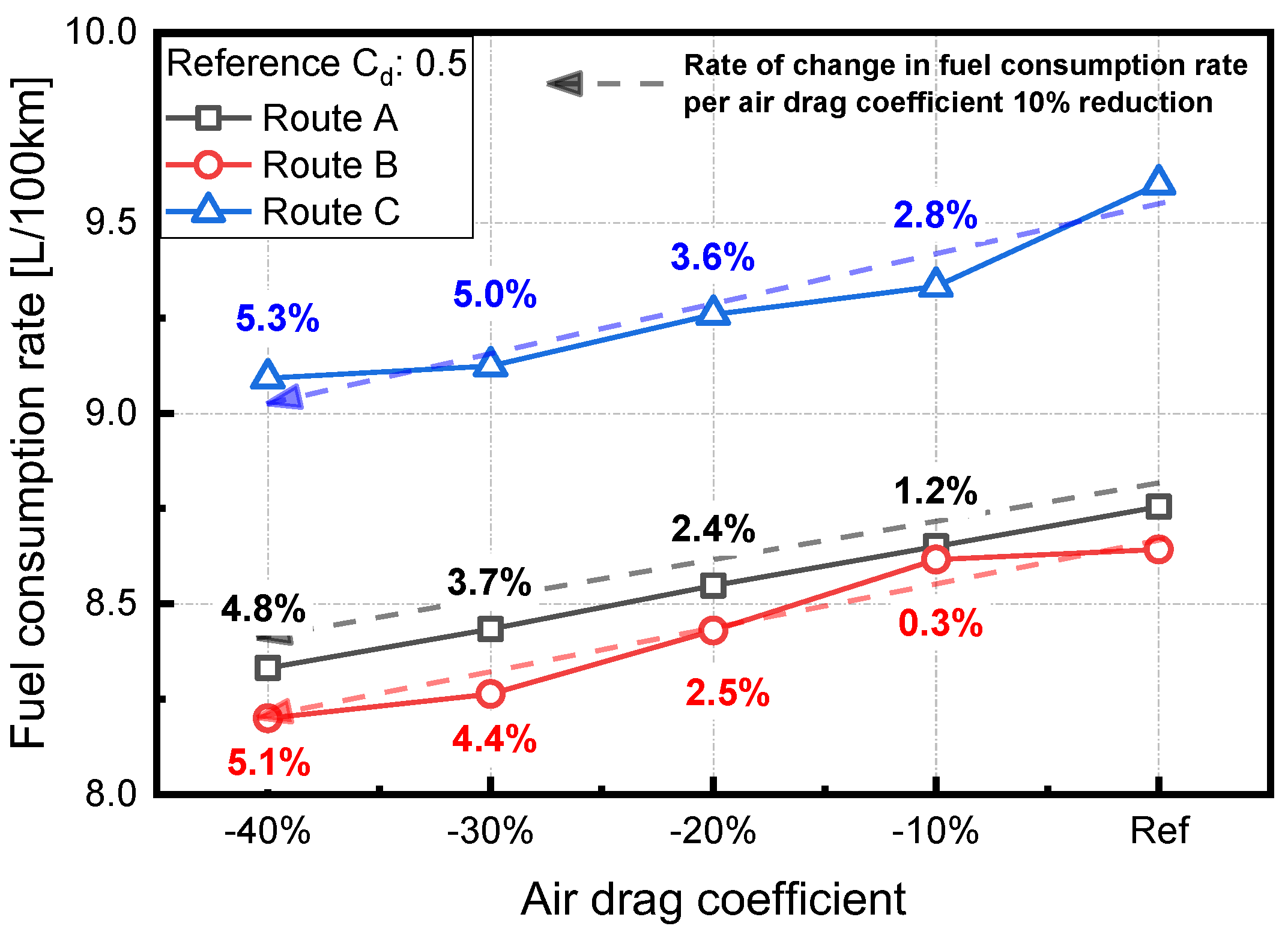
Figure 8 shows the fuel consumption rate with respect to the air drag coefficient. The air drag coefficient corresponds to the coefficient of form for the flow of air. As the air drag coefficient decreases, the air resistance decreases. If the air resistance decreases and driving resistance decreases, then fuel economy improves because the vehicle can be driven at a relatively low output. In 2020, the highest temperature in Korea corresponded to 33.9 °C, and the lowest temperature corresponded to −17.5 °C. Furthermore, air density increases by approximately 20% if the temperature decreases by the aforementioned temperature difference under atmospheric pressure. Additionally, techniques such as changes in vehicle geometry can reduce the air drag coefficient by approximately 10%. Therefore, it is assumed that the air drag coefficient decreases by 40% compared to the reference value. This factor multiplied by the area of the front of the vehicle is proportional to the aerodynamic drag and is calculated as follows [12]:
(ρ: air density (kg/m3), Cd: drag coefficient, A: frontal area (m2), and V: vehicle velocity (m/s)).
As shown in Equation (4), aerodynamic drag is proportional to the square of the vehicle speed; aerodynamic drag typically corresponds to the dominant factor in driving resistance at speeds exceeding 100 km/h, while there is a threshold when the dominant factor changes to rolling resistance within the range of 50–100 km/h. The threshold is dependent on the structure and weight of the vehicle [18]. This implies that aerodynamic drag is relatively more important in high-speed sections than in low-speed sections.
In Figure 8, higher fuel efficiency is observed on Route B with a higher driving ratio on the highway section than other routes. Furthermore, based on the values applied during feasibility validation on all routes, the decreases in the air drag coefficient by 10% improved the fuel consumption rate. However, the fuel efficiency improvement rates were similar for the three routes. This means that the fuel efficiency, according to the air drag coefficient, was not affected by the route characteristics. In particular, there is no difference in the fuel efficiency improvement rate despite the difference in the average speed between the three routes. This is attributed to the fact that aerodynamic drag does not significantly affect driving resistance given that the maximum vehicle speed on all routes corresponded to 85 km/h. The cause is also related to the analysis of the effect on the ratio of the valid window ratio in Figure 9.
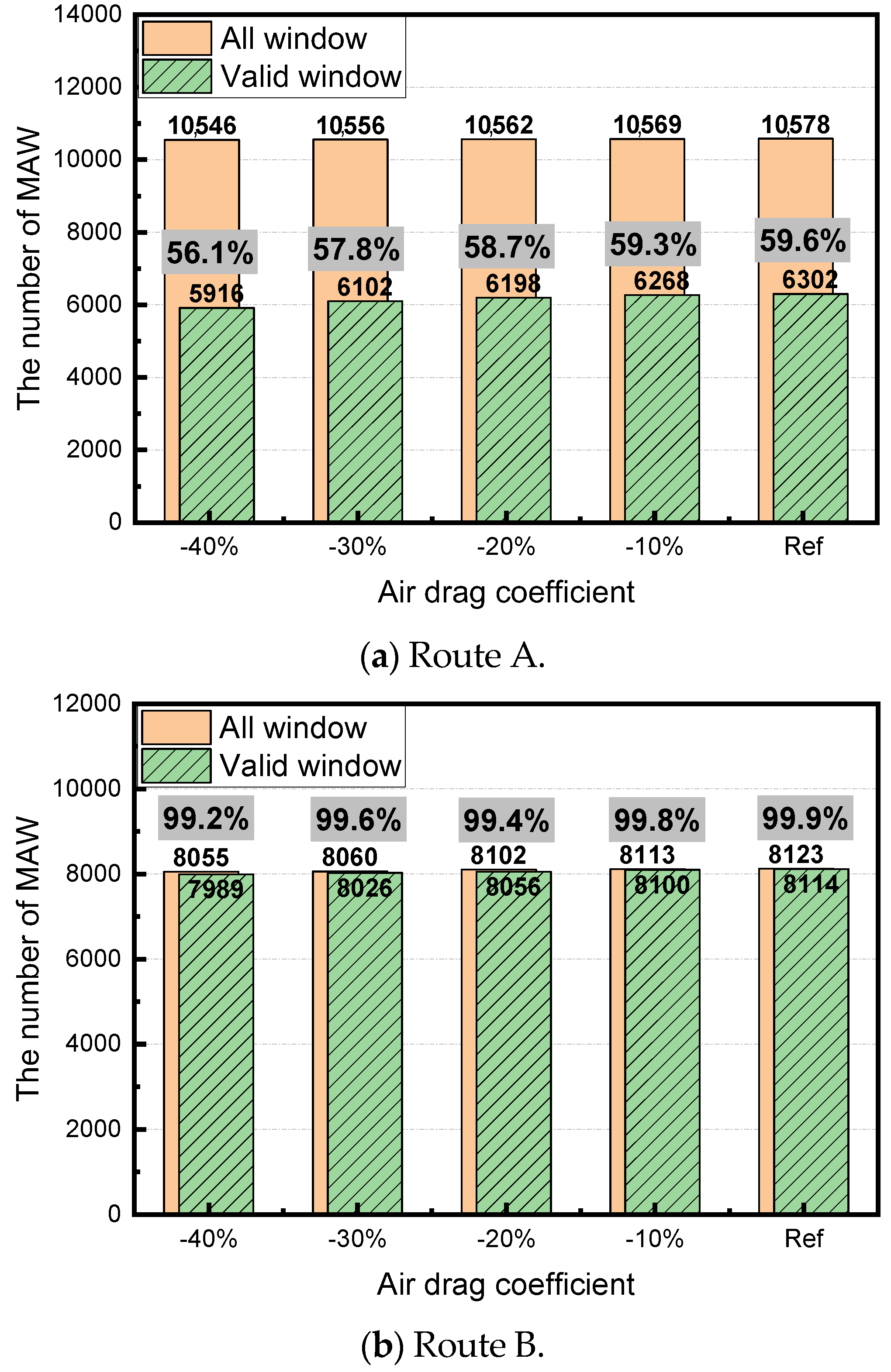
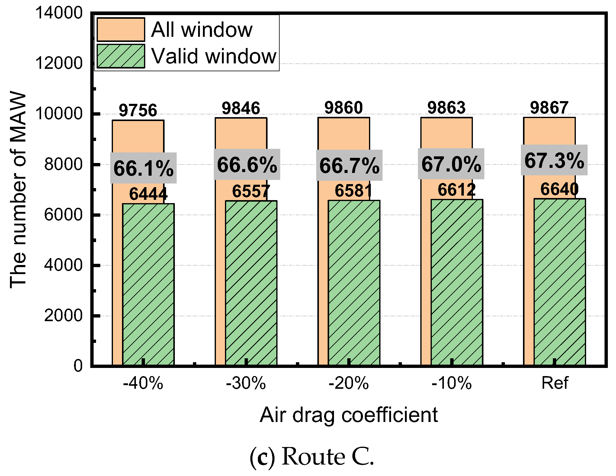
Figure 9 shows the number of moving average windows according to the air drag coefficient and the ratio of the valid window. When the air drag coefficient decreased by 40% compared to the reference value, the ratio of the valid window decreased by 3.5, 0.7, and 1.2% in Routes A, B, and C, respectively, and no test was observed as invalid. This means that the change in the required engine output compared to the reduction rate of the aerodynamic drag coefficient is not large. Thus, the reduction rate in the ratio of the valid window compared to the fuel efficiency improvement rate can be determined as low. For example, a reduction in the payload for Route A from 50 to 40% improves fuel consumption by 6.4% and lowers the valid window ratio by 7.2%, thereby indicating that a 5.1% improvement in fuel consumption decreases the valid window ratio by approximately 5.7%. In comparison, a decrease in the air drag coefficient by 40% compared to the reference value improves fuel consumption by 5.1% and decreases the valid window ratio by 3.5%. Thus, if the driving speed is low, then the reduction in the fuel efficiency improvement rate due to decreases in the air drag coefficient is not significant. However, if the fuel efficiency improvement rate is the same, the decrease rate of the valid window can be reduced.
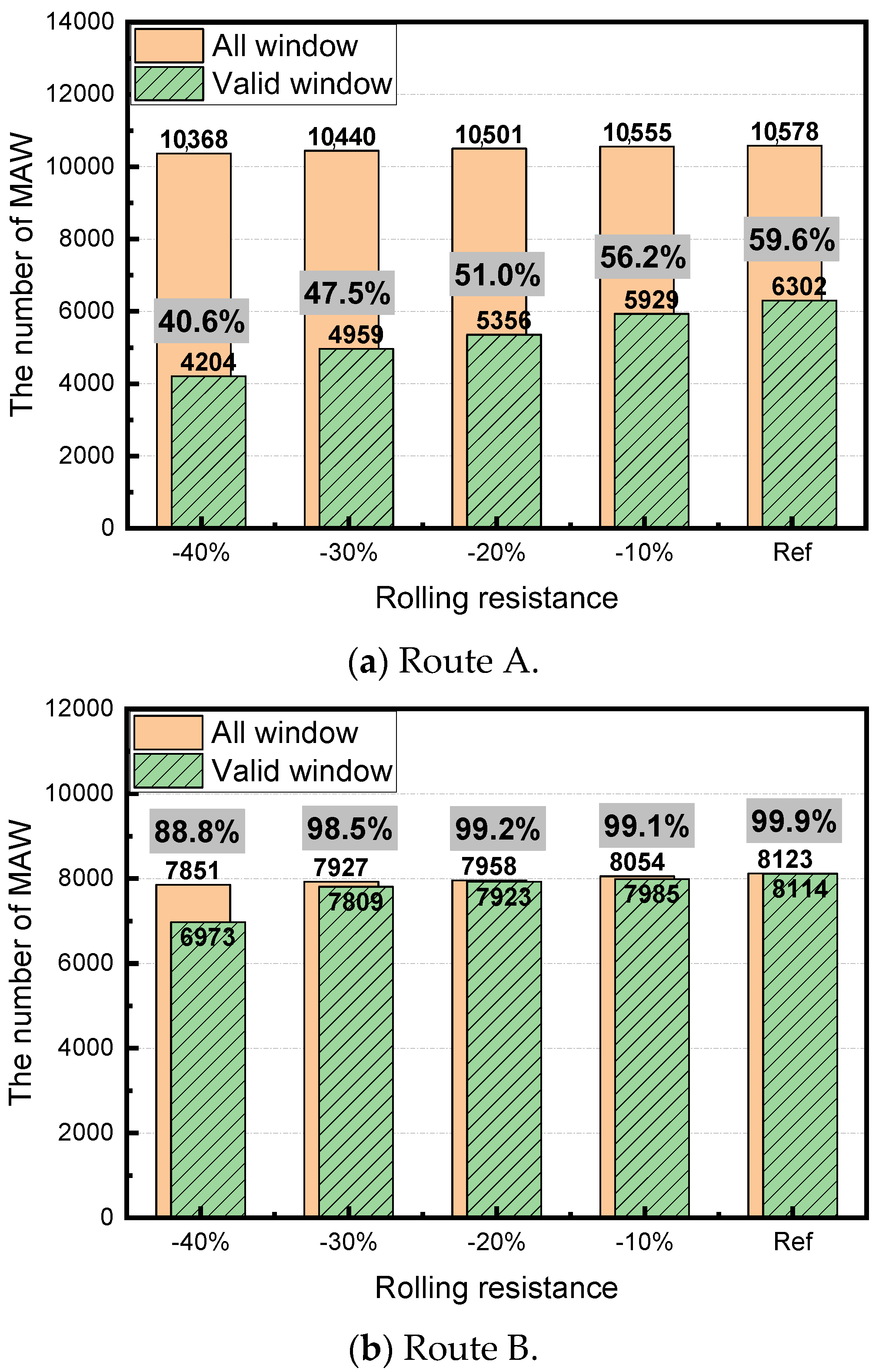
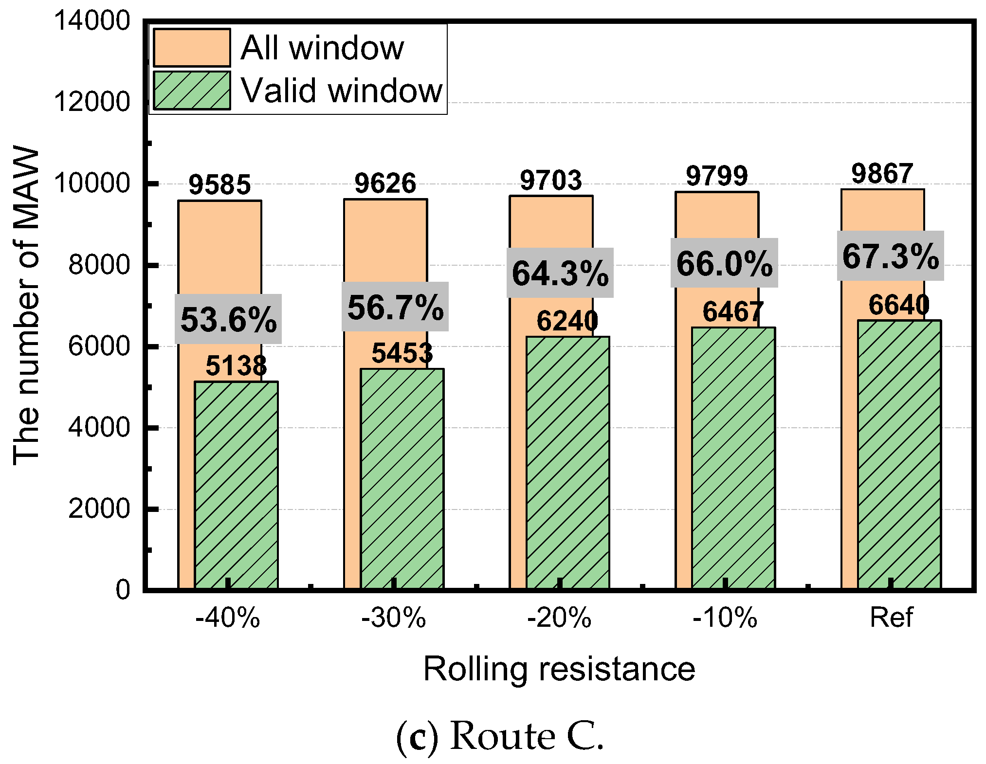
3.4. Fuel Consumption Rate and Valid Window Ratio according to the Rolling Resistance
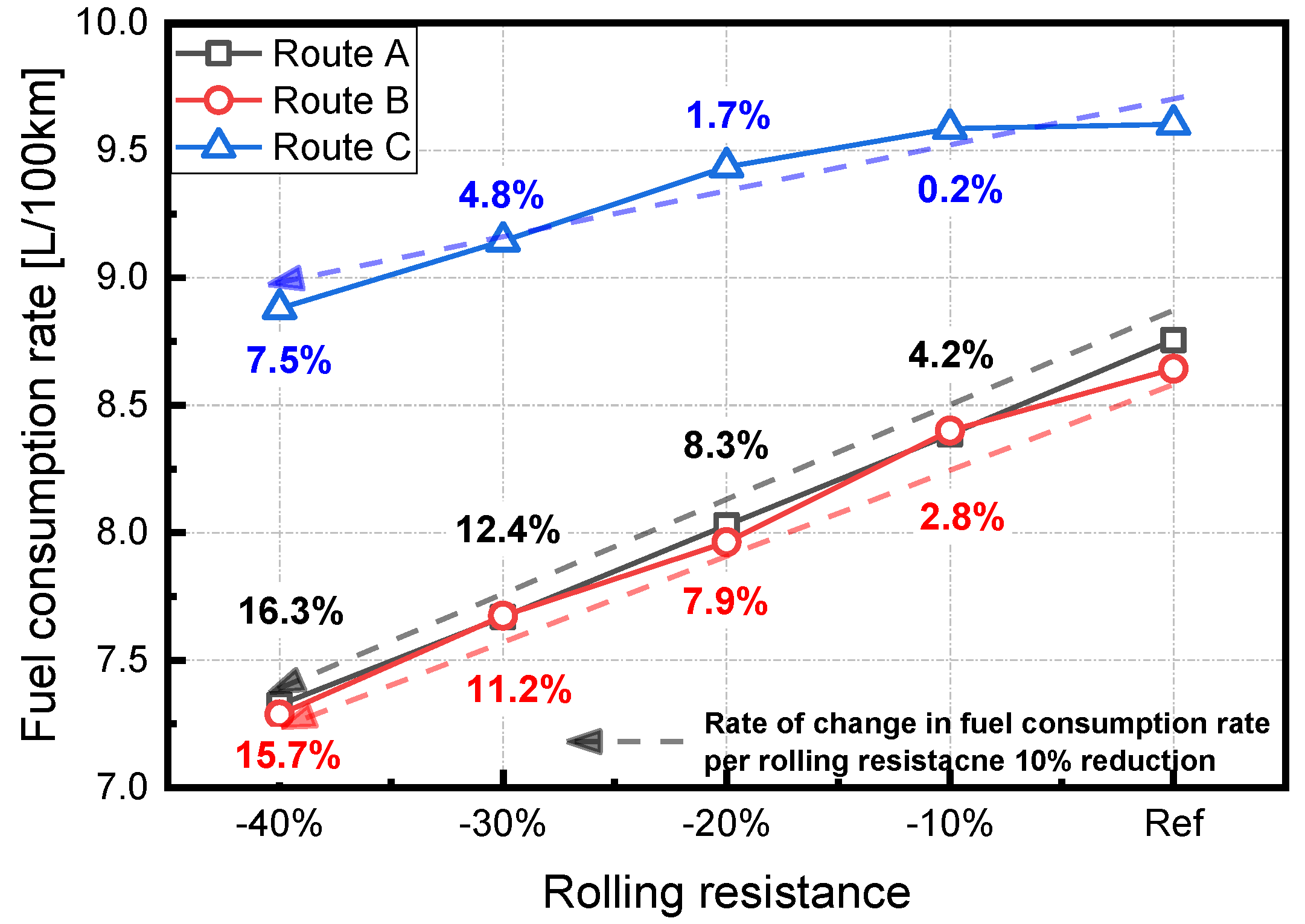
Figure 10 shows the rate of fuel consumption due to rolling resistance. In the study, we assume that rolling resistance does not change with respect to vehicle speed. As shown in the figure, as the rolling resistance decreases by 10% based on the value applied during feasibility validation, the fuel consumption rate is improved. If the rolling resistance decreases by 40% compared to the reference value, then the fuel consumption rate for Routes A, B, and C improves 16.3, 15.7, and 7.5%, respectively, which, in turn, exceeds the effect of the air drag coefficient. It is considered that rolling resistance is relatively higher than the air drag coefficient because, as previously mentioned, the rolling resistance generally corresponds to the dominant factor in driving resistance, as opposed to aerodynamic drag, if the vehicle speed does not exceed 100 km/h in general. The rolling resistance factor is affected by tire air pressure, speed, and load. Specially, it is significantly affected by tire air pressure [19]. Therefore, fuel economy can be easily improved by decreasing rolling resistance via increasing tire air pressure.
Figure 11 shows the number of moving average windows according to the rolling resistance and the ratio of the valid window. When the rolling resistance decreased by 40% compared to the reference value, the ratio of the valid window decreased by 19%, 11.1%, and 13.7% in Routes A, B, and C, respectively. This implies that decreases in rolling resistance for Route A can significantly decrease engine power and driving resistance compared to those in other routes. This, in turn, can lead to a relatively significant improvement in fuel consumption, as shown in Figure 10. This is considered to be highly influenced by rolling resistance because Route A exhibits a large elevation difference and gradient for the same distance compared to other routes. Additionally, if the rolling resistance decreases below 30% in Route A, then the ratio of the valid window is less than 50%, and the test can be considered as invalid. The reduction rate in the ratio of the valid window to the fuel efficiency improvement rate due to reduced rolling resistance was less than that when the payload decreased, while it was higher than that when the air drag factor decreased. For example, if the payload is decreased in Route A and the fuel consumption rate is improved by 8.5%, then the valid window ratio is reduced by approximately 9.6%. If the rolling resistance is decreased by 20% compared to the reference value, then the fuel consumption is improved by 8.5%, and the valid window ratio is decreased by 8.6%. Therefore, if the driving velocity is low, then the reduction in the rolling resistance can be more effective in improving fuel economy than a reduction in the air drag coefficient. Furthermore, the decrease rate in the ratio of the valid window can be reduced further compared to that in lowering the payload.
4. Conclusions
In this study, large vehicle powertrains were modeled using AVL Cruise, and real driving data were subsequently applied to predict fuel consumption rates and the ratio of the valid window. Hence, the effect of the payload, air drag coefficient, and rolling resistance on fuel economy and test suitability for three driving routes was quantitatively analyzed.
- As the payload, air drag coefficient, and drag resistance decreased, the fuel consumption rate improved, and the ratio of the valid window decreased. When the payload decreased from 50 to 10% based on the maximum payload, the fuel consumption rate in Route A improved by 32.5%, and the ratio of the valid window decreased by 26.9%. However, when the payload was reduced, the transport efficiency deteriorated. In addition, it was confirmed that the effect of the payload on the valid window ratio varies depending on the route characteristics.
- When the gradient variation of the driving route was small, and the ratio of highway section was high (Route B), the ratio of the valid window was relatively high. In addition, the fuel efficiency in accordance with the payload, air drag factor, and rolling resistance was higher than other routes.
- As the driving speed decreases, the fuel efficiency improvement rate decreases due to decreases in the air drag coefficient. However, with respect to a case of the same fuel efficiency improvement rate, the reduction in the air drag coefficient was less proportional to the valid window than the reduction in the payload.
- In the case of heavy-duty trucks with many tires (the contact area of the tire is large), as the driving speed decreased, the rate of fuel efficiency improvement due to the rolling resistance increasing. If the rate of improvement due to rolling resistance is maintained as constant, then the effect on the ratio of the valid window was lower than that on the payload and higher than that on the air drag coefficient.
- Using a 1D simulation program, it was confirmed that by setting the appropriate payload, air resistance, and rolling resistance, the probability of failure of the test can be decreased, and additional time and cost can be decreased. In the future, we will analyze the valid window characteristics of each road section because the current MAW method does not reflect the pollutant emissions in the urban section.
Author Contributions
All authors contributed to the experiments, analysis, and the deployment of the paper. Conceptualization, data curation, investigation, methodology, writing—original draft, S.J. and H.J.K.; data curation, investigation, S.I.K.; methodology, resources, J.T.L.; funding acquisition, resources, S.P. and J.T.L.; supervision, writing—review and editing, S.P. All authors have read and agreed to the published version of the manuscript.
Funding
This study was financially supported by the Transportation Pollution Research Center in the National Institute of Environmental Research (NIER-2021-04-02-27), AVL Cruise UPP (University Partnership Program), and the Basic Science Research Program (2019R1A2C1089494) through the National Research Foundation of Korea (NRF), funded by the Ministry of Education (Korea).
Data Availability Statement
The data that support the findings of this study are available from the corresponding author upon reasonable request.
Conflicts of Interest
The authors declare no conflict of interest. The funders had no role in the design of the study; in the collection, analyses, or interpretation of data; in the writing of the manuscript, or in the decision to publish the results.
References
- European Commission. White Paper—Roadmap to a Single European Transport Area—Towards a Competitive and Resource Efficient Transport System; European Commission: Brussels, Belgium, 2011. [Google Scholar]
- Greenhouse Gas Inventory and Research Center. Available online: http://www.gir.go.kr/home/index.do?menuId=36 (accessed on 29 December 2016).
- European Environment Agency. Available online: https://www.eea.europa.eu/publications/carbon-dioxide-emissions-from-europes (accessed on 12 April 2018).
- Masjuki, H.H.; Azman, S.S.N.; Zulkifli, N.W.M.; Syahir, A.Z. Tribology: It’s Economic and Environmental Significance. Mytribos Symp. 2017, 2, 1–3. Available online: https://mytribos.org/mytribossymposium/resources/MTS2-1-3.pdf (accessed on 21 February 2021).
- Kousoulidou, M.; Fontaras, G.; Ntziachristos, L.; Bonnel, P.; Samaras, Z.; Dilara, P. Use of portable emissions measurement system (PEMS) for the development and validation of passenger car emission factors. Atmos. Environ. 2013, 64, 329–338. [Google Scholar] [CrossRef]
- Duarte, G.O.; Gonçalves, G.A.; Farias, T.L. Analysis of fuel consumption and pollutant emissions of regulated and alternative driving cycles based on real-world measurements. Transp. Res. Part D Transp. Environ. 2016, 44, 43–54. [Google Scholar] [CrossRef]
- Wang, Y.; Ge, Y.; Wang, J.; Wang, X.; Yin, H.; Hao, L.; Tan, J. Impact of altitude on the real driving emission (RDE) results calculated in accordance to moving averaging window (MAW) method. Fuel 2020, 277, 117929. [Google Scholar] [CrossRef]
- Tietge, U.; Mock, P.; German, J.; Bandicadekar, A.; Ligterink, N. Real-World Vehicle Fuel Consumption Gap in Europe at All Time High; International Council on Clean Transportation: Washington, DC, USA, 2017. [Google Scholar]
- Su, S.; Ge, Y.; Hou, P.; Wang, X.; Wang, Y.; Lyu, T.; Luo, W.; Lai, Y.; Ge, Y.; Lyu, L. China VI heavy-duty moving average window (MAW) method: Quantitative analysis of the problem, causes, and impacts based on the real driving data. Energy 2021, 225, 120295. [Google Scholar] [CrossRef]
- Wang, Y.; Hao, C.; Ge, Y.; Hao, L.; Tan, J.; Wang, X.; Zhang, P.; Wang, Y.; Tian, W.; Lin, Z.; et al. Fuel consumption and emission performance from light-duty conventional/hybrid-electric vehicles over different cycles and real driving tests. Fuel 2020, 278, 118340. [Google Scholar] [CrossRef]
- Katreddi, S.; Thiruvengadam, A. Trip Based Modeling of Fuel Consumption in Modern Heavy-Duty Vehicles Using Artificial Intelligence. Energies 2021, 14, 8592. [Google Scholar] [CrossRef]
- Zeng, I.Y.; Tan, S.; Xiong, J.; Ding, X.; Li, Y.; Wu, T. Estimation of Real-World Fuel Consumption Rate of Light-Duty Vehicles Based on the Records Reported by Vehicle Owners. Energies 2021, 14, 7915. [Google Scholar] [CrossRef]
- Fontaras, G.; Rexeis, M.; Dilara, P.; Hausberger, S.; Anagnostopoulos, K. The Development of a Simulation Tool for Monitoring Heavy-Duty Vehicle CO2 Emissions and Fuel Consumption in Europe; SAE Technical Paper: Warrendale, PA, USA, 2013; No. 2013-24-0150. [Google Scholar]
- Srinivasan, P.; Kothalikar, U.M. Performance Fuel Economy and Co2 Prediction of a Vehicle Using Avl Cruise Simulation Techniques; SAE Technical Paper: Warrendale, PA, USA, 2009; No. 2009-01-1862. [Google Scholar]
- Ko, K.-H.; Choi, S.-C. A study on the improvement of vehicle fuel economy by fuel-cut driving. J. Korea Acad. Coop. Soc. 2012, 13, 498–503. [Google Scholar]
- Choi, J.; Jeong, J.; Lee, D.; Shin, C.; Park, Y.-I.; Lim, W.; Cha, S.W. Analysis of Fuel Economy Sensitivity for Parallel Hybrid Bus according to Variation of Simulation Input Parameter. Trans. Korean Soc. Automot. Eng. 2013, 21, 92–99. [Google Scholar] [CrossRef] [Green Version]
- Fan, S.; Lee, J.; Sun, Y.; Ha, J.; Harber, J. Virtual Platform Development for New Control Logic Concept Test and Validation. SAE Technical Paper: Warrendale, PA, USA, 2021; No. 2021-01-1143. [Google Scholar]
- Tilvaldyev, S. Review of Aerodynamic Drag Reduction Devices for Heavy Trucks and Buses; Instituto de Ingenieríay Tecnología: Chihuahua, Mexico, 2020. [Google Scholar]
- Lee, B.; Kim, D.; Lee, J.; Cha, W.; Seo, Y. Influence of Tire Rolling Resistance Coefficient on Road Load and Fuel Economy for Passenger Car. Trans. Korean Soc. Automot. Eng. 2018, 26, 745–754. [Google Scholar] [CrossRef]
Figure 1.
Image of the AVL Cruise heavy-duty vehicle model.

Figure 2.
Test vehicle dynamics and dimensions.

Figure 3.
Post process of the fuel efficiency map.

Figure 4.
Time-dependent vehicle velocity profile for each route.

Figure 5.
Comparison of fuel efficiency between experiment and simulation results for Route A.

Figure 6.
Fuel consumption rate with respect to payload for each route.


Figure 7.
Number of MAWs and the ratio of the valid window with respect to payload for each route.

Figure 8.
Fuel consumption rate with respect to air drag coefficient.

Figure 9.
Number of MAWs and the ratio of the valid window with respect to air drag coefficient for each route.
Figure 9.
Number of MAWs and the ratio of the valid window with respect to air drag coefficient for each route.


Figure 10.
Fuel consumption rate with respect to rolling resistance.

Figure 11.
Number of MAWs and the ratio of the valid window with respect to the rolling resistance for each route.
Figure 11.
Number of MAWs and the ratio of the valid window with respect to the rolling resistance for each route.


Table 1.
Specification of the test vehicle.
| 8 × 4 Rigid Body Truck | |
|---|---|
| Vehicle curb weight | 13,590 kg |
| Vehicle gross weight | 35,000 kg |
| Maximum payload | 25,007 kg |
| Frontal area | 7.76 m2 |
| Wheel static rolling radius | 482 mm |
| Wheel dynamic rolling radius | 522 mm |
Table 2.
Specification of the test engine.
| Engine Type | 6-Cylinder Diesel Engine |
|---|---|
| Bore | 123 mm |
| Stroke | 152 mm |
| Displacement | 10,837 cm3 |
| Compression ratio | 17:1 |
| Idle speed | 500–700 rpm |
| Maximum speed | 2150 rpm |
| Maximum power | 339 kW @ 1700–1800 rpm |
| Maximum torque | 2200 Nm @ 1050–1400 rpm |
Table 3.
Driving characteristics of each route.
| Route A | Route B | Route C | |
|---|---|---|---|
| Driving distance | |||
| Urban | 30 km | 20.6 km | 20.3 km |
| Rural | 35 km | 31.6 km | 36.5 km |
| Highway | 102 km | 128.9 km | 106.1 km |
| Total | 167 km | 181.1 km | 162.9 km |
| Driving time | |||
| Urban | 3775 s | 2180 s | 3808 s |
| Rural | 2887 s | 1620 s | 2167 s |
| Highway | 5829 s | 6113 s | 5137 s |
| Total | 12,491 s | 9913 s | 11,112 s |
| Average vehicle velocity | |||
| Urban | 28.6 km/h | 34 km/h | 19.2 km/h |
| Rural | 48.4 km/h | 70.2 km/h | 60.6 km/h |
| Highway | 63 km/h | 75.9 km/h | 74.4 km/h |
Disclaimer/Publisher’s Note: The statements, opinions and data contained in all publications are solely those of the individual author(s) and contributor(s) and not of MDPI and/or the editor(s). MDPI and/or the editor(s) disclaim responsibility for any injury to people or property resulting from any ideas, methods, instructions or products referred to in the content. |
© 2023 by the authors. Licensee MDPI, Basel, Switzerland. This article is an open access article distributed under the terms and conditions of the Creative Commons Attribution (CC BY) license (https://creativecommons.org/licenses/by/4.0/).
Share and Cite
MDPI and ACS Style
Jo, S.; Kim, H.J.; Kwon, S.I.; Lee, J.T.; Park, S. Assessment of Energy Consumption Characteristics of Ultra-Heavy-Duty Vehicles under Real Driving Conditions. Energies 2023, 16, 2333. https://doi.org/10.3390/en16052333
AMA Style
Jo S, Kim HJ, Kwon SI, Lee JT, Park S. Assessment of Energy Consumption Characteristics of Ultra-Heavy-Duty Vehicles under Real Driving Conditions. Energies. 2023; 16(5):2333. https://doi.org/10.3390/en16052333
Chicago/Turabian StyleJo, Seongin, Hyung Jun Kim, Sang Il Kwon, Jong Tae Lee, and Suhan Park. 2023. "Assessment of Energy Consumption Characteristics of Ultra-Heavy-Duty Vehicles under Real Driving Conditions" Energies 16, no. 5: 2333. https://doi.org/10.3390/en16052333
Note that from the first issue of 2016, this journal uses article numbers instead of page numbers. See further details here.