
Use of Magnetostrictive Actuators for Wave Energy Conversion with Improvised Structures

Environmental Health and Engineering Department, Johns Hopkins University, Baltimore, MD 21218, USA
Energies 2023, 16(4), 1835; https://doi.org/10.3390/en16041835
Submission received: 14 December 2022
/
Revised: 3 February 2023
/
Accepted: 4 February 2023
/
Published: 12 February 2023
(This article belongs to the Special Issue Wave Energy: Theory, Methods, and Applications)
Abstract
:This paper presents work on a wave energy device with an on-board power take-off based on a magnetostrictively actuated deformable structure. Such devices potentially could be used in low-cost, short-term expeditionary operations. The paper discusses an analytical model that describes the heave oscillations of a buoy with two inclined, overhanging beams with magnetostrictive strips affixed to them. This work comprises the first steps toward an analytical model that would enable potential users to obtain quick power estimates at the planning stage. Here, the fully nonlinear magneto-mechanical-electrical constitutive relations are linearized about a desirable operating point, and a coupled dynamic model is derived using a variational formulation that includes buoy heave, flexural oscillations of the two beams, and the voltage response of the magnetostrictive strips. Energy conversion performance in wind-sea-dominated Pierson–Moskowitz spectra is found to be modest. However, present results also indicate that performance could be improved with suitable mechanical modifications.
1. Introduction
Wave energy utilization has interested inventors and potential users since at least the late 19th century. Several archetypal conversion technologies that have developed since then are reviewed in [1]. Principles and components of several conversion concepts are reviewed in [2], while some hydrodynamics and control-related aspects of representative conversion methods are described in [3]. Interest in wave energy conversion has grown significantly in recent years, with much of the activity being aimed at commercial-sale applications [4]. Use of wave energy for powering oceanographic instrumentation has also received increasing attention (e.g., [5,6]) in recent years. There is now a growing body of work focused on a variety of non-grid applications of wave energy with commercial potential (e.g., [7]), and progress is also being made in the design of wave energy converters for recharging autonomous underwater vehicles (AUV) [8].
Whereas much of the present-day research emphasizes device technologies that are intended to serve for several years and meet the power conversion requirements for long-term applications, this paper presents a somewhat different perspective. Here, we describe a part of our recent research on small, improvised wave energy devices that are expected only to serve temporary short-term needs. Particular focus is on the use of low-cost indigenous materials, straightforward assembly and operation, minimal hardware, and where applicable, single-use primary converter with multi-use power take-off systems that are interchangeable among different primary converters.
Such considerations may arise in a variety of situations in including recreational activities such as seaside camping, sailing, and fishing expeditions where there are limits on transportable hardware and when small amounts of power are desired from environmental sources such as waves. Certain applications may also require quiet operation.
The need for quiet operation and interchangeability precludes a number of mechanical options for the power take-off. Here, we investigate a power take-off based on deformable structures and ‘smart’ materials for which structural strain produces an electrical (in addition to mechanical) response and vice versa. Piezoelectric materials have been considered for secondary energy conversion in wave energy conversion since at least the late eighties [9]. Recent trends in application of piezoelectric materials for wave energy conversion can be found, for instance, in [10]. Due to their small coupling coefficients, piezoelectrics lack the force authority to serve as effective power converters in applications where large amounts of power with large forces and displacements are involved [11]. This is particularly true for piezoelectric polymers being used to control flexural deformations [12]. The question considered in this work was whether metallic smart materials could effectively serve the force and displacement needs of wave energy conversion. Rare-earth metal alloys such as Terfenol (terbium–dysprosium–iron) and Galfenol (gallium–iron) are known to have magnetostrictive properties (e.g., [13,14]). Accordingly, these materials deform structurally when subjected magnetic fields. A reverse effect also occurs when an external force produces a structural deformation that causes a magnetic field, which in turn leads to a voltage and current. Magnetostrictive materials have been tested for application in energy harvesting [14] as well as structural vibration control [15], which provides the motivation for investigating them for energy conversion and oscillation control on wave-actuated deformable structures that could potentially constitute the power take-off system for a small wave energy device. The emphasis of the present work is on the energy conversion potential of magnetostrictive materials for a small wave energy device. It is expected that magnetostrictive strips manufactured in large numbers would present a cost advantage. Potential users could then use a selected number for power conversion with deformable structures on an improvised wave energy device.
In the case of Galfenol or Terfenol actuators, an externally applied magnetic field between the two ends of a magnetostrictive strip aligns the internal magnetic moments along the field direction. When such a strip is deformed in a direction normal to the field, the structural deformation causes the moments to realign, which in turn alters the magnetic flux density across a conductor coil around the strip, producing a voltage and driving a current through a load. For Galfenol and Terefenol, the effect can be bidirectional and it enables actuation and sensing, and our goal here is to investigate whether it is strong enough to enable power capture from waves. In particular, we consider the energy capture performance of a power take-off based on long, flexible beams affixed with strips of Galfenol, whose magnetostrictive properties are well documented and readily available (e.g., [14]).
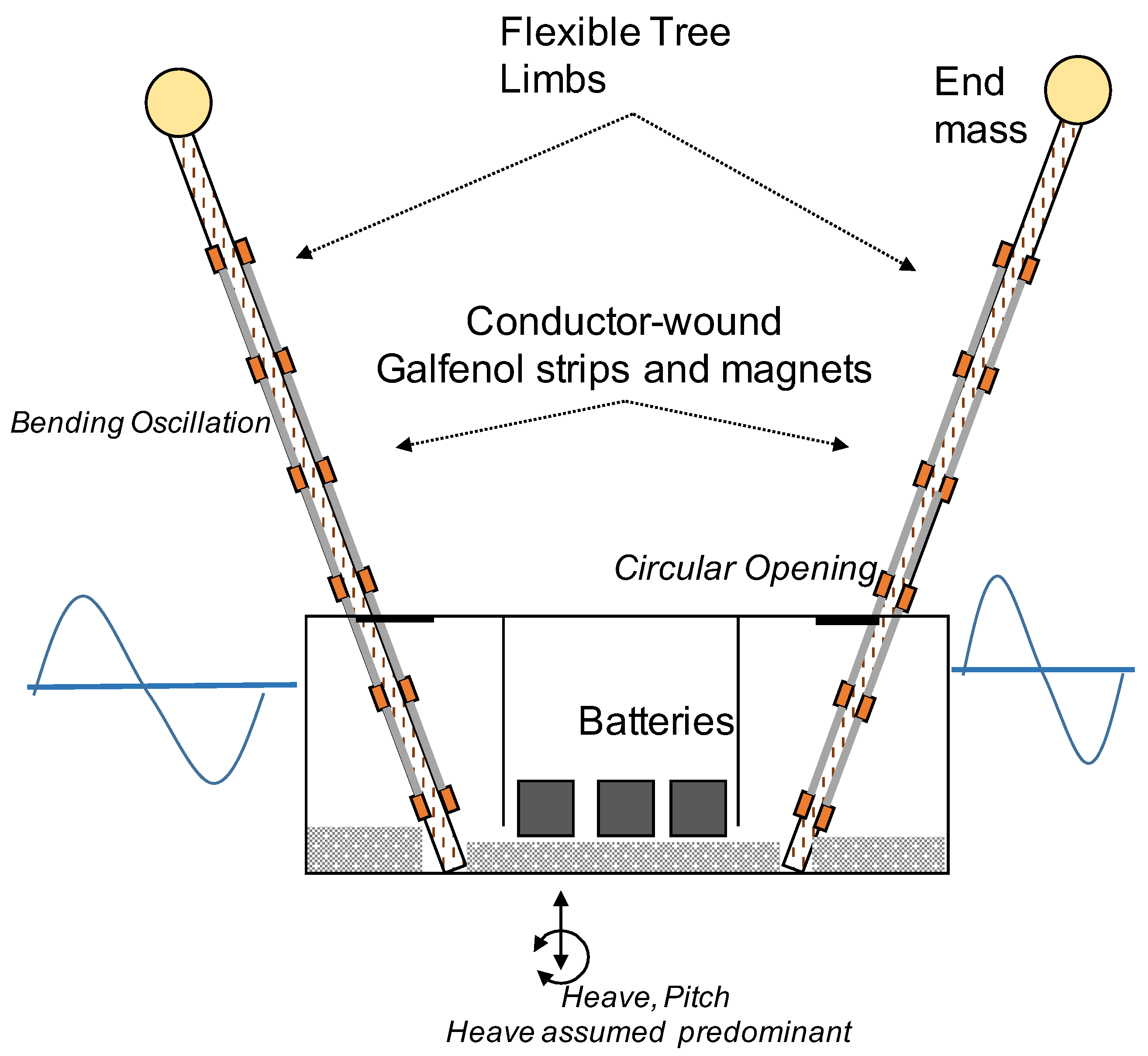
The relationships that quantify structural response to magnetic fields and vice versa are an extension of the ‘constitutive relations’ from structural mechanics. Here, the constitutive relations are derived from a full magneto-electro-mechanical description, as reviewed in [13]. The two important goals of the present work are, (i) to develop an integrated dynamic model for a system comprised of a wave excited body that carries on board two long beams with Galfenol strips affixed to them; and (ii) to use a constitutive model for Galfenol that allows material behavior nonlinearities to be utilized to improve actuation authority and power capture. Figure 1 shows a schematic for a small buoy with the Galfenol actuated long beams, potentially assembled using tree limbs. A cylindrical geometry is chosen here because it is amenable to 3-D printing technology, and can even be assembled by tying together a number of tree logs. Wave motion causes the buoy to oscillate. Buoy oscillations excite oscillations of the two beams, which in turn cause cyclic deformation of the Galfenol strips attached to the beams. Each beam carries an end-mass at its overhanging ends, the purpose of the end masses being to accentuate the low-frequency oscillations of the beams, knowing that ordinary wind-wave or swell spectra would apply excitation in the frequency range from 0.1 to 1 Hz.
Section 2.1 describes the magnetostrictive constitutive relations used in this work. Section 2.2 discusses the dynamic model for the wave-excited buoy with long beams supporting Galfenol strips. Section 3 discusses The paper concludes with a summary of the main findings in Section 4.
2. Materials and Methods
2.1. Magnetostriction Constitutive Relationships
The following treatment is based on [13]. It is assumed that the magnetostrictive strips are prestressed to a stress , which induces a magnetic field (the middle term in Equation (1) below). The externally applied magnetic field is related to the current I flowing through the coil around the strip and the number of turns N. The overall magnetic field on the strip can be expressed as,
where accounts for coil end effects, and is approximated as here. M denotes magnetization, while and are saturation magnetostriction and saturation magnetization, respectively. is free-space magnetic permeability, and quantifies the effect of interactions between magnetic moments. The magnetization M is comprised of an anhysteretic component and an irreversible component , as
If the oscillations occur over a small portion of the curve about an operating point , then the irreversible component can be neglected. can be expressed as
To find the dynamic relationship between M and , we use the expansion
Combining Equations (1) and (3) and using the approximation (4), we can express the magnetization M as
The combined strain at a point x on the beam due to a stress T and magnetization M can be expressed as
Here, s denotes compliance (i.e., reciprocal of stiffness). For oscillations about the operating point , in the second term can be linearized as
Letting denote the prestrain in the beam due to the steady magnetic field ,
denoting just the oscillatory part of the strain as S,
Denoting as H, with the understanding that must be small, and defining its coefficient as d,
To find the direct relationship between the magnetic flux density B and the stress T, we argue that the component of B due to the stress-caused magnetic field component is
denotes the permeability at constant stress. Approximating conditions with H held constant at (with ),
With the derivative of with respect to T defined as ,
The full expression for magnetic flux density B together with the direct contribution of H can be written as
Note that Equations (12) and (16) are linear, and form the constitutive relationships we use here, although the operating point can be chosen to maximize magnetostriction (and thus the mechanical to electric coupling), with d and being evaluated at the operating point.
The coefficients in Equation (17) are given by
2.2. Coupled Dynamic Model
The dynamic model for the problem at hand is summarized below. The situation being modeled is interesting in that we have floating-body oscillations being excited by waves, with the oscillations in turn exciting the oscillations of the flexible beams with magnetostrictive actuators attached. Thus, between the waves and the electric circuit powered by the actuator current and voltage, there are three energy exchanges: (i) between waves and floating body, (ii) floating body and oscillating beams, and (iii) beam oscillations to converter electrical circuits. The boundary conditions for the overhanging beams are summarized below.
2.2.1. Boundary Conditions
The tree limb beams shown in Figure 1 are resting on the keel of the buoy, with part of their weight also being supported by the deck openings through which they overhang. Here, the two supports are modeled as pin joints, and the tree limbs are modeled as two-span beams with one span of length overhanging a shorter simply supported span of length . For either beam of length , with denoting the out-of-plane beam deformation at a point x along beam length, we may define , and to express the beam profiles for a solution as follows.
Additionally, we allow below for the endpoints of the beam overhangs also to support an end masses to accentuate beam oscillations at the lower frequencies common to ordinary wave spectra. The boundary conditions become
above represents the end mass carried by each beam, and represents the flexural rigidity of the beams with Galfenol strips attached. is defined in the following section. The boundary conditions in Equation (20) present a closed system, with the determinant going to zero at the spatial eigenvalues of the overhanging beams. From these, the natural frequencies of the beams can be determined for various geometries and end-masses, with the goal of finding the best combinations for the present application.
Two cases are studied below: (1) where the deck-level supports for the beams are tight enough for the beams to maintain contact with them throughout the oscillation; and (2) where these supports are loose enough for the beams to bounce within the supports during their oscillation cycles.
For convenience, the buoy shape is chosen to be cylindrical with a hemispherical bottom. Heave is assumed to be the dominant oscillation, even though a pitch/roll mode can be added relatively easily. For the case with the tight deck-level supports, the dynamic variables are (i) buoy oscillation in heave s, (ii) beam oscillations in single-axis bending , and (iii) voltage produced between the terminals of an electrical load circuit connected to the actuators V. A third variable representing the beam angle was added to the system for the situation with loose supports. It was found convenient to use the variational formulation for deriving the equations of motion for the entire system.
2.2.2. Beams Tightly Fitting through Deck Supports
For the first case, the angle between the beams and the vertical was assumed to be a constant, . For the beams, uniaxial bending is assumed, and shear deformation and rotary inertia are neglected. The total kinetic energy was expressed as
The in-air mass of the buoy is , while represents its infinite-frequency added mass in heave. is the mass of each beam, and is the end-mass attached to each beam. Further, is the deflection of the ith beam perpendicular to its neutral axis, the vertical deflection component being given by . The strain at any beam fiber z from the neutral axis can be expressed as for small deflections. Then, using this expression for S in Equation (17), the total potential energy of the beams together with the potential energy of the buoy can be expressed as
Here, denotes the second derivative with respect to x of , the out-of-plane deflection of the ith beam. The Lagrangian is
An action variable J can be set up over a time interval such that
Minimization of J over the interval requires that the first variation . The minimization process leads to the equations of motion and the boundary conditions (natural or externally prescribed), which we here prescribe as in Equation (20) above. The equations of motion can be derived from
The force on the right side of the first of Equation (25) represents the exciting/diffraction force due to waves, the radiation force due to body oscillation in waves, and additional effects such as viscous-frictional damping.
The equation of motion for the buoy is
on the right denotes the exciting force (accounting for diffraction effects) due to waves. The convolution integral on the left is part of the radiation force, with denoting the impulse response of the body. represents the linear approximation to the viscous friction damping force. Next, the equation of motion for the ith beam is found to be
We point out here that the flexural rigidity term in Equation (20) is given by
The magnetic flux density is further related to the deflection through
It is noted next that the voltage produced across the coil wound around the Galfenol actuators is related to the magnetic flux density according to
We assume that (which includes changes due to flowing current) remains approximately constant during the oscillation for small oscillations and for a long coil of conductors over a strip. Therefore, its spatial and temporal derivates are approximated to zero. Then,
Then, if the coil on each strip spans from to , we find that the voltage difference between the two terminals of the coil is
Equation (33) provides the voltage that would be available for use during the oscillation. Since Equation (27) uses oscillation components in the vertical direction, substitution for as expressed in Equation (31) implies
Equations (26) and (34) describe the overall oscillation dynamics, with the waves imparting a predominantly heave oscillation on the buoy and the buoy acceleration then driving the beam deflections. Each of the Galfenol strips attached to the beams respond with a voltage difference between two ends of a conductor coil wound around it, as described by Equation (33). The beam oscillations are consistent with the boundary conditions in Equation (20). With a load resistor connected across the conductor coil in a simple implementation, the power dissipated by it would be
Buoy displacement and beam deflections can be evaluated when the wave-applied exciting force on the body is known. In this work, the time series were obtained for chosen irregular wave conditions, assuming long-crested Pierson–Moskowitz spectra. The spectral density was computed knowing the significant wave height and energy period , after which a wave elevation time series could be computed assuming superposition of a large number of frequencies (in this work, for most calculations) with the phase angles provided by a random number generator.
It is relatively straightforward to solve Equations (26) and (34) as a system by expanding the deflection into its natural modes or eigenfunctions as determined by the boundary conditions (20). Thus, letting
where are the time-dependent modal oscillations, and
We note that the modes are mutually orthogonal. Expanding in Equation (34) for each beam into its eigenfunctions, multiplying both sides by and integrating from 0 to L, and utilizing the orthogonality property of the nth eigenfunction , we arrive at the following ordinary differential equations for each modal displacement . This process results in the following system of equations.
Here,
This formulation allows N to be a suitably large number. In this application, the source of excitation is surface waves, whose action is mostly confined to the frequency range Hz, which corresponds to a wave period range of s. In light of this, it is argued that only the fundamental flexural modes of the present beams would be responsive to oscillations in the practical surface wave frequency range. We therefore just include the fundamental modes, so that . Retaining just the first oscillation modes for the beams and taking the Fourier transforms of both sides of each remaining equation,
Here, , , and are all complex-valued. The exciting force , frequency-dependent added mass , and the radiation damping , etc., can be evaluated for a given geometry, using a numerical solver for a boundary-element type approximation. Equation (40) thus represent a system of algebraic equations which yields frequency-domain solutions for , , and . The voltage across the conductor coil can then be determined and the power converted can be computed knowing the load resistor (or equivalent resistance in a load circuit being driven by the power take-off).
2.2.3. Beams Loosely Held within Deck Supports
In this case, the large clearance between the beams and the deck supports allows beam rotation about the points where they rest on the keel. As the buoy oscillates, it excites rigid body rotations of the beams that repeatedly are interrupted by impacts with the deck-support inner edges. Each impact acts as an impulsive load causing flexural vibrations over a range of natural modes. We expect that repeated excitation of some of the flexural natural modes may enhance power conversion beyond what is available through the fundamental-mode flexural vibration mode examined above. The dynamics of the overall system with this additional feature are modeled as described below.
In addition to the three main variables, , , and above, there are now variables and that represent the rigid-body rotations of the beam about the rest-angle , which is set to be the same for each beam, and each beam has a length L. In this case, the beam end-masses also play an important role in the overall response. Further, in addition to the buoy exciting force , there are now impact forces that act on the beams each time they collide with the inner periphery of their respective deck openings. The total kinetic energy of the system can be expressed as the sum of the following:
The potential energy of the system is the sum of
Assuming the rigid-body rotations of the beams to be small, the boundary conditions of Equation (20) are assumed to continue to be valid for this case too. The Lagrangian for this case is expressed as
Here, and . The external forces acting on the buoy in this case are the same as for the previous case. However, each impact causes an impulsive force to act on the beams that needs to be accounted for. Using Lagrange’s equations as outlined in Equation (23) and assuming two beams, we arrive at the set of equations that describe the overall dynamics, starting with
for the buoy heave. Here, includes the exciting force in heave on the buoy due to waves and the radiation force as in Equation (26) above. The additional force here is the force generated each time a beam impacts its support during its oscillation. An expression for this force is given following the remaining equations of motion. For the rigid-body rotation of each beam, we have (assuming that , )
Next, for the flexural oscillation of each of the beams, we have
The impact force occurs each time the oscillating beam strikes the loose support, or at each when
is the length of the short span of the beam (recall that a length overhangs the support and that ). The magnitude of can be expressed as
The equivalent mass of the beam can be derived, for the fundamental oscillation mode, as
Once again, expanding the beam flexural oscillation into its eigenfunctions as in Equation (36) and for the moment, retaining just the fundamental mode, we arrive at the following system of equations. For buoy heave , we have
Here, and are as defined above, including also
and is given by Equation (48), occurring at each when the condition (47) is satisfied. The equation of motion for becomes
Finally, the flexural mode is described by
In the results discussed here, a reduced version of the model in Equations (50)–(53) was tested, for quicker indications of the benefit of the proposed loose-fitting arrangement. The successive impacts were modeled using a series of Dirac delta function in the time-domain, and it was assumed that the impact-generated flexural oscillations decayed rapidly. In the frequency domain, the overall effect of successive impacts was approximated using the force
denotes the peak frequency in a spectrum. In the present calculations, the displacement of the beam relative to the buoy was assumed to be in phase for , and opposite in phase for . denotes the wave-applied exciting force at the peak frequency .
3. Results and Discussion
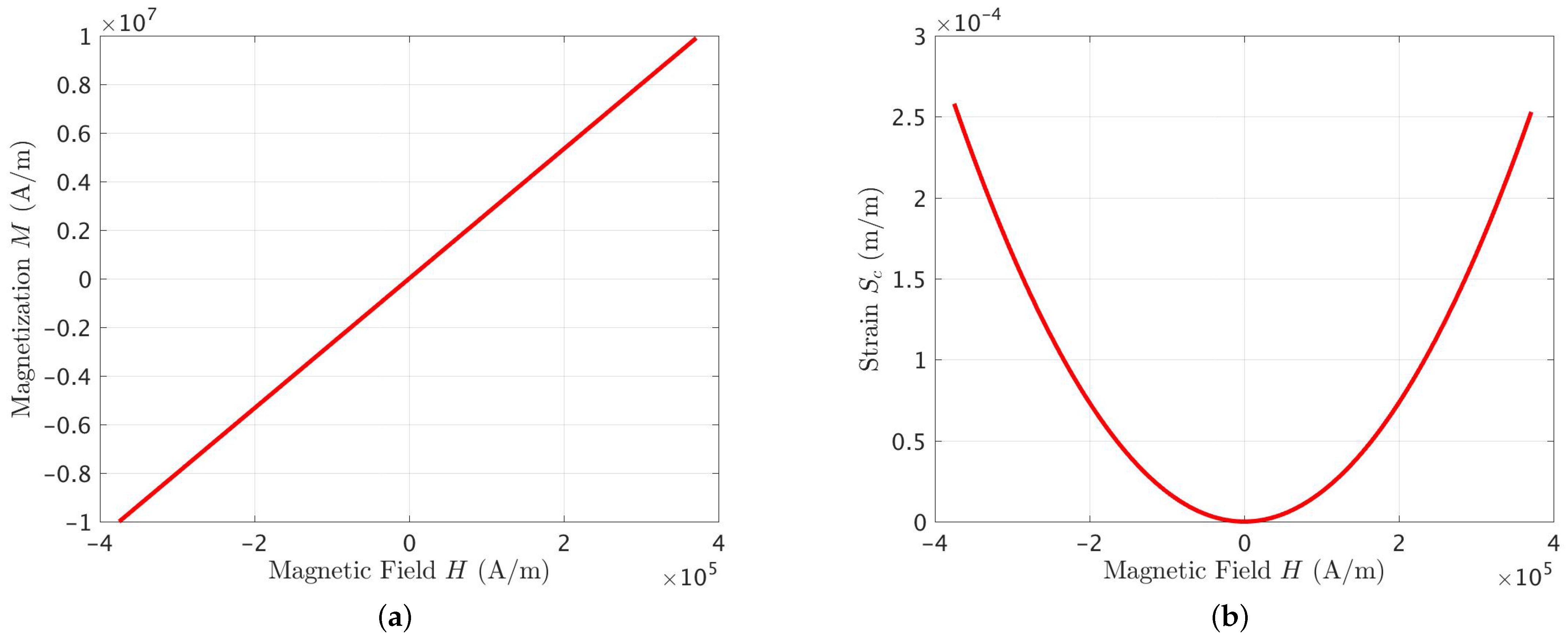
Figure 2a plots the anhysteretic part of the magnetic field-magnetization relationship. The mostly linear relationship flattens as the magnetic field intensity increases beyond the values shown [13]. Figure 2b plots the essence of the magnetostrictive effect as described by the relationship between applied magnetic field and resulting strain. We note the growing slope of the curve with increasing H.
A review of Figure 2 suggests that an operating point about a large value of H (> A/m) would likely be ideal for prestraining the present actuators. A large value for prestraining would imply greater slope of the curve, which would mean greater strain for smaller changes in the magnetic field, or conversely, greater changes in magnetic field for smaller changes in strain.
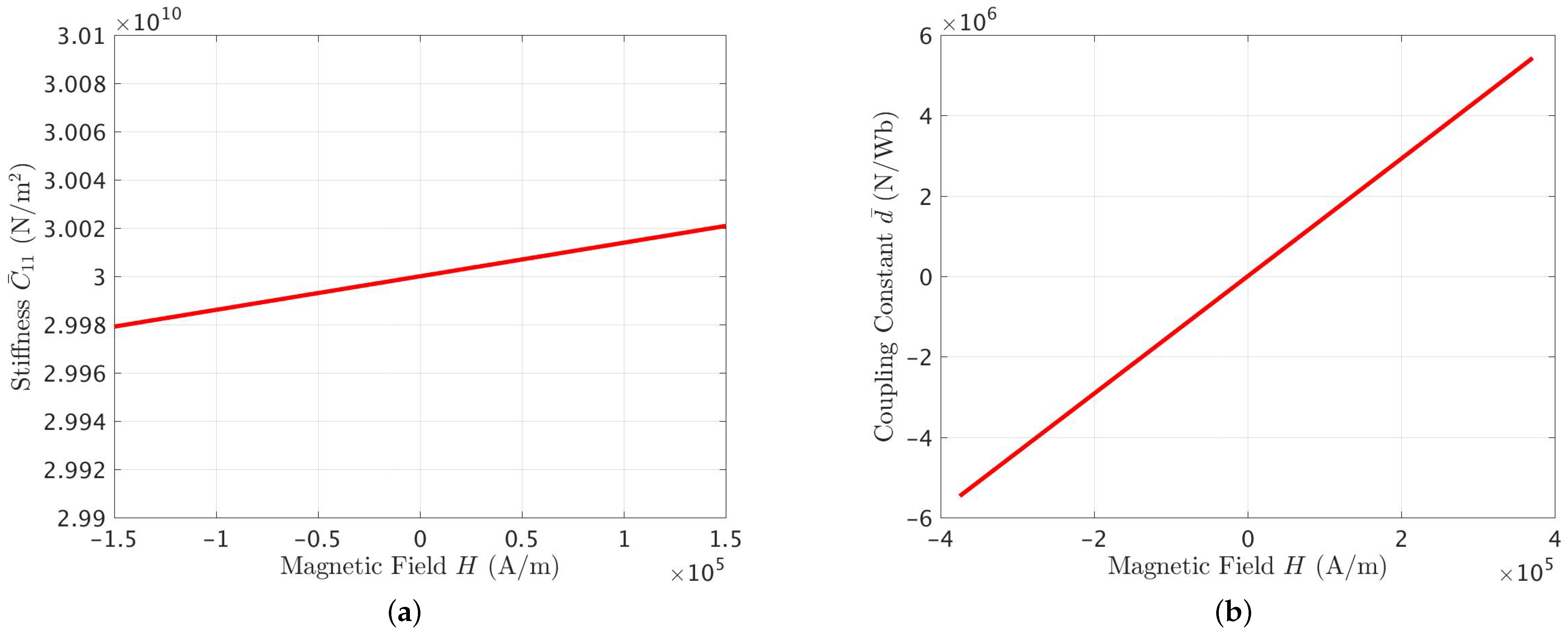
The following figures refer to the stress–strain–magnetic field–magnetic flux density relationships as linearized about the chosen . The goal was to explore whether, by changing the applied magnetic field , we could significantly alter the values of any of the coupling constants in the linearized constitutive relationships. An ability to do so would enable real-time control of the response of a magnetostrictive actuator (i.e., make it more sensitive to strain or magnetic flux density by changing the field during operation). These relationships are reviewed in Equation (55) below.
The coupling coefficients and are shown in Figure 3. These describe, respectively, how the magnetic field can influence the coupling between strain and stress, and the coupling between magnetic flux density and stress. As Figure 3a shows, is not particularly sensitive to changes H. Hence, it does not seem profitable to attempt magnetic field manipulation to change the stiffness of a magnetostrictive actuator during service. On the other hand, it appears that the coupling constant can be adjusted considerably during operation by changing , although this was not attempted in the present work.
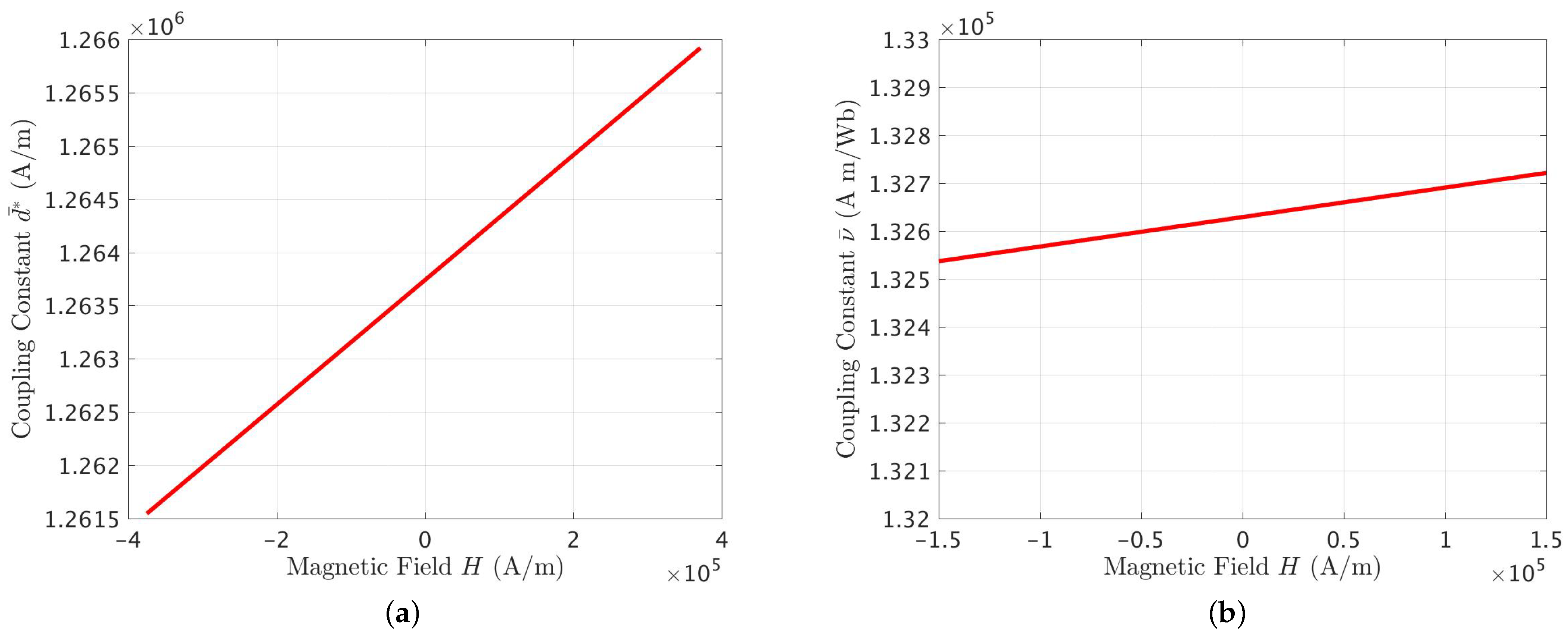
Figure 4 plots the coefficients and that relate, respectively, the strain to the magnetic field H and the magnetic flux density to the magnetic field in the presence of magnetostriction. Neither coefficient is found to be particularly sensitive to , which indicates that the magnetostriction property of the material is not very strong. Although can be changed considerably by altering , its small magnitude implies small magnitudes for the magnetic flux density (and the voltage) produced during oscillations.
The dynamic performance of the complete system was investigated in real-sea conditions. Results for a Pierson–Moskowitz wave spectrum with significant wave height m and energy period s are discussed below. Although only wind seas are considered to be dominant in these calculations, a Pierson–Moskowitz spectrum is helpful because of the relative ease with which swell and wind seas can be combined in simulations. As mentioned previously, two cases were studied: (i) with the beams tightly fitting within the deck-level openings, and (ii) with the beams supported supported loosely within the deck-level openings, so that they would experience repeated impacts as they oscillate.
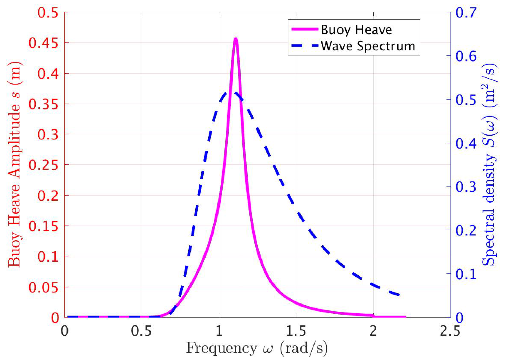
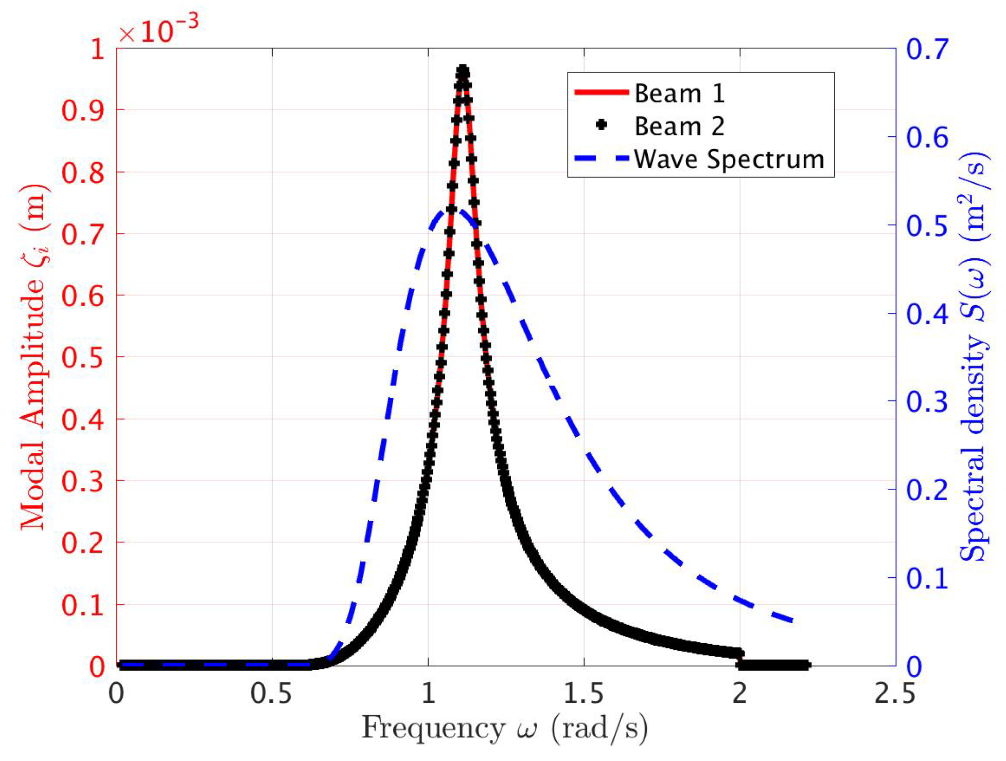
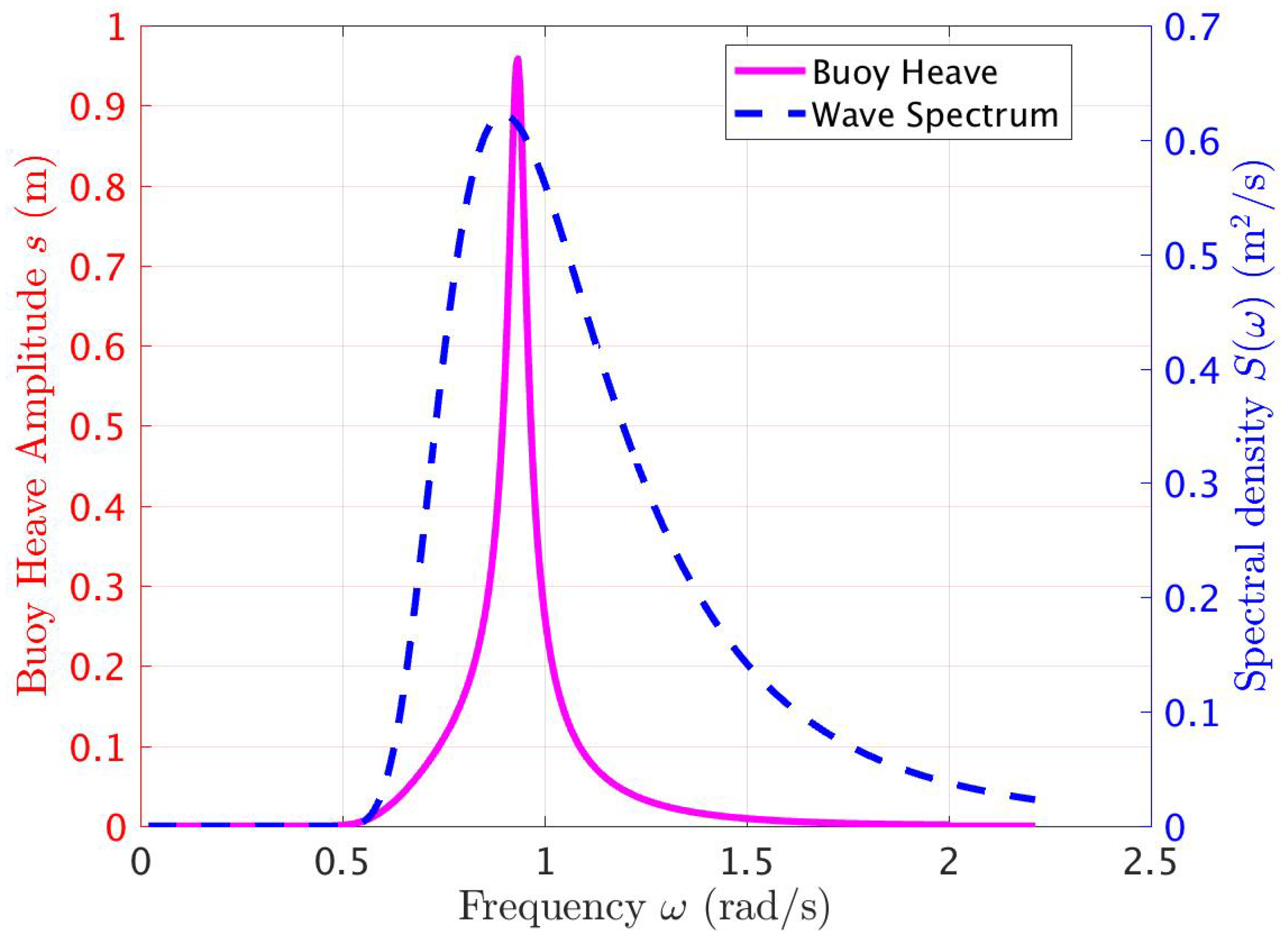
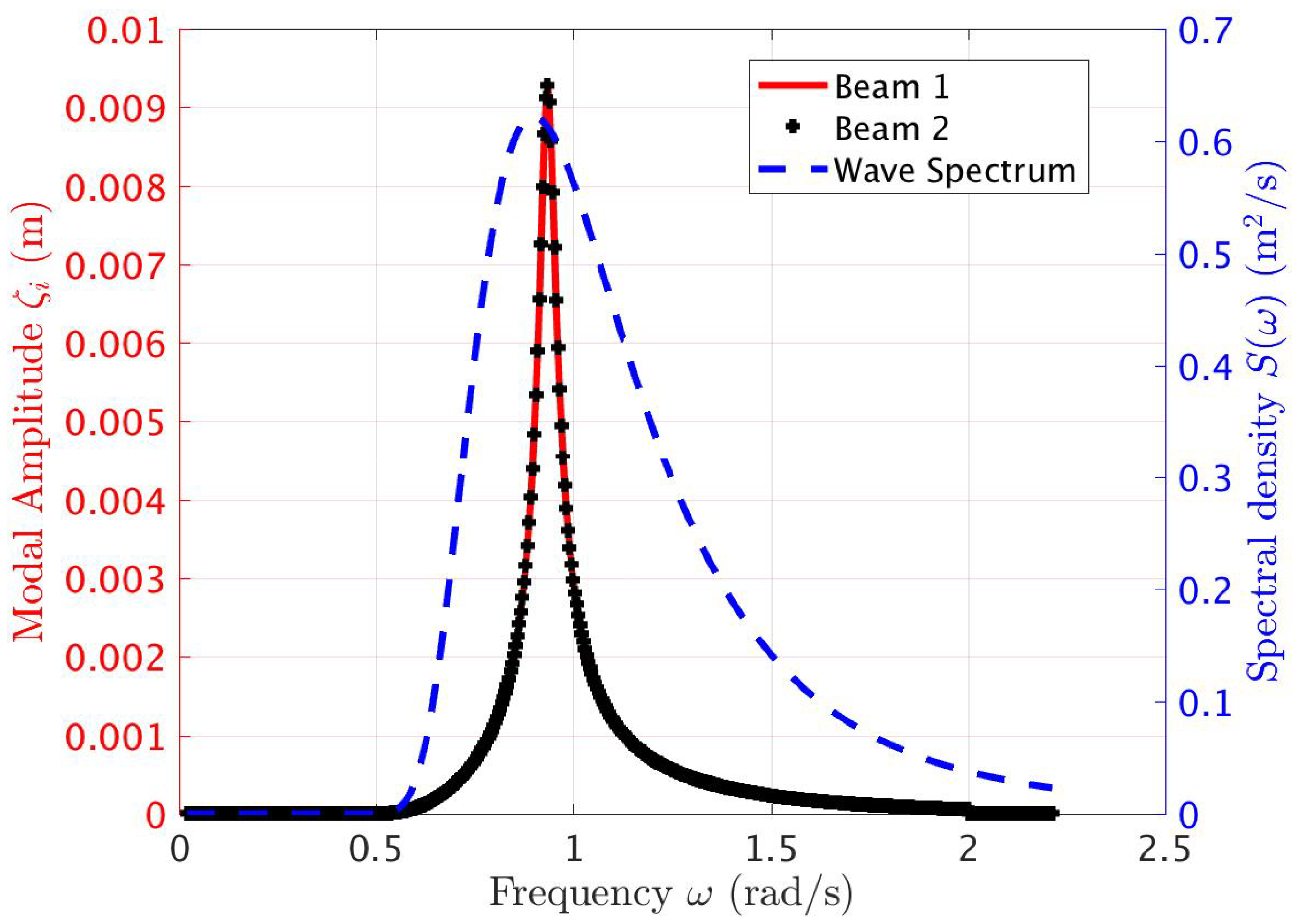
Case (i) results are considered first. Figure 5 shows the buoy heave amplitude frequency response, with a peak at rad/s and amplitude 0.45 m. Given the small diameter of the buoy (2.0 m), the displacement response is narrow-banded, despite the coupling with the two beams on deck. Figure 6 plots the flexural oscillation fundamental mode amplitudes and for the beams, with a peak at rad/s. The coupled system comprising a buoy and beams has a peak response at rad/s. Also shown in Figure 5 and Figure 6 is the power spectral density used in the calculations. It is observed from these figures that the dynamic response of the device is reasonably well-matched to the wave conditions.
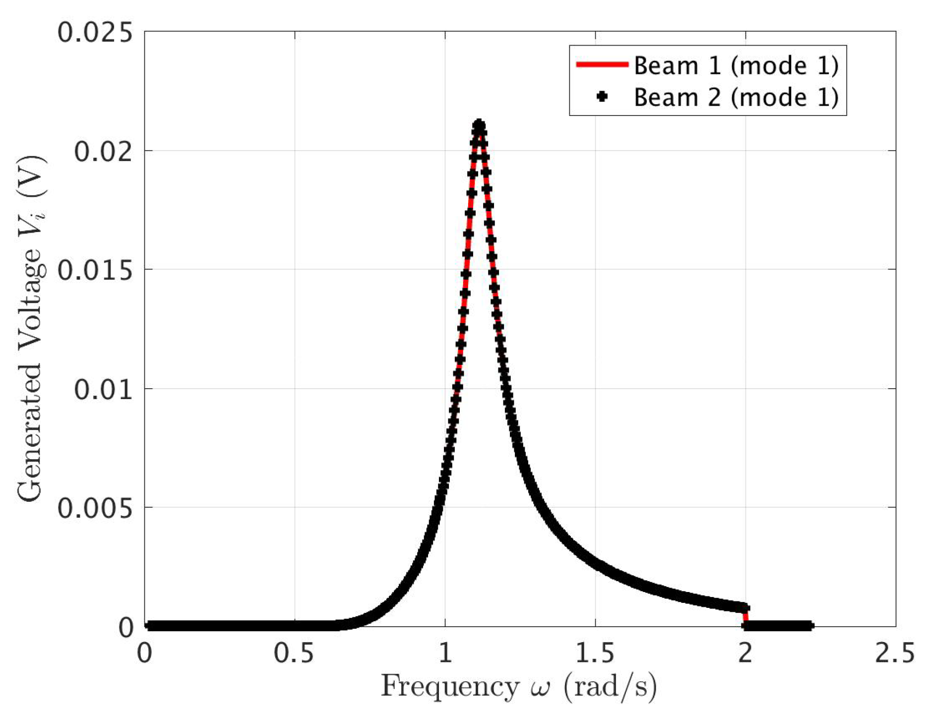
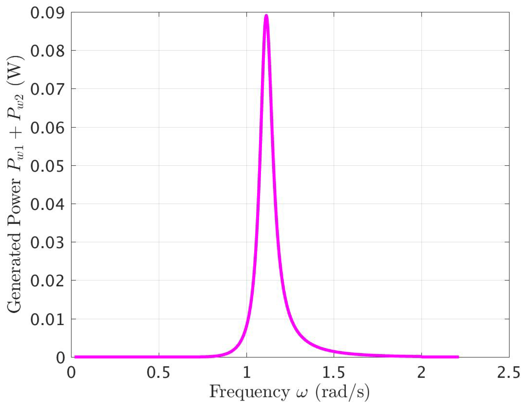
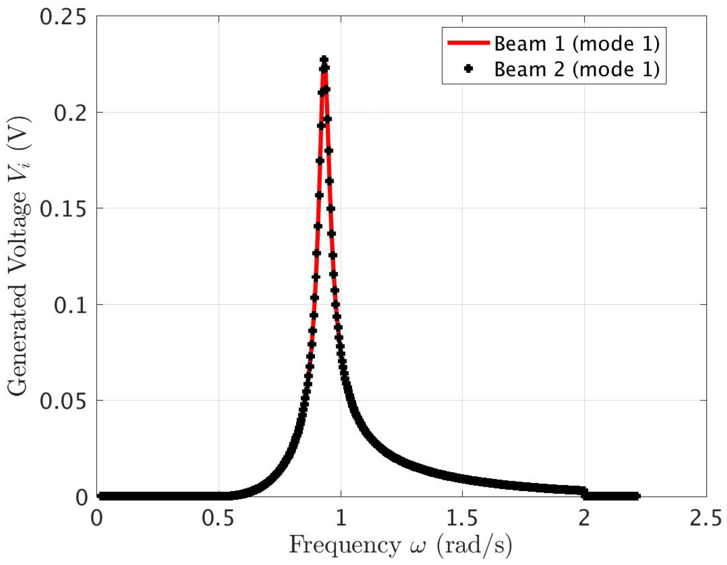
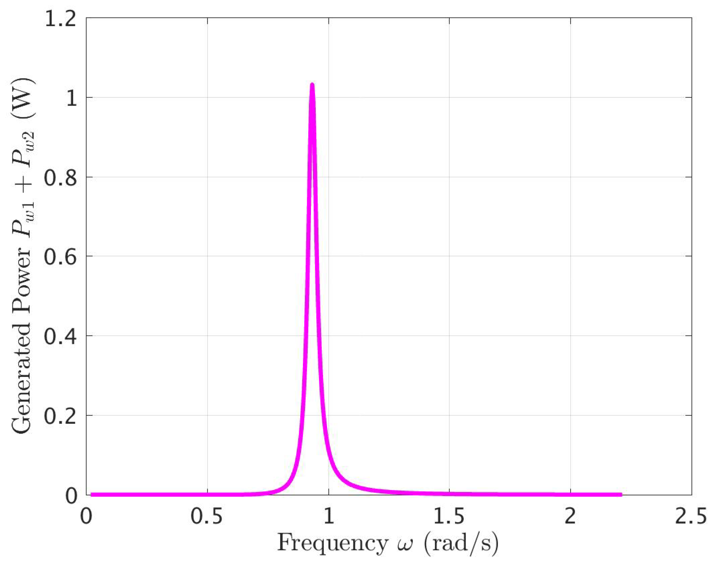
Figure 7 shows the voltage between terminals for each of the two beams. Each beam is equipped with a single, long Galfenol strip, with a coil of 20,000 conductor turns and a load resistance of 0.01 ohm. The number of conductor turns is roughly 7 per millimeter, which is practically feasible with thin conductor wires. The combined power converted by the two strips (one on each beam) is shown in Figure 8. Both voltage and power values are found to be small, with peaks around 25 mV and 90 mW, respectively. Attaching M Galfenol strips to each beam, as well as providing more beams, would raise the power outputs overall, while adding to the system mass, which could be helpful in improving the low-frequency response and power conversion from waves.
Note that the small jump in the curves near rad/s occurs because the numerically determined radiation damping value is truncated to zero beyond this frequency.
Case (ii) results are discussed next. As Figure 9 shows, the peak response amplitude of the buoy is slightly greater for the same wave spectrum as before, while the fundamental-mode oscillations of the beams are also greater (Figure 10). Beam oscillations are found to be considerably greater in this case.
As noted, the voltage and power results of Figure 11 and Figure 12, respectively, considerable improvement is observed in both, particularly at frequencies closer to the natural frequencies of the beams. Thus, each Galfenol strip is now seen to generate about 80 mV at the spectral peak, while the converted power at the peak frequency now exceeds 1.2 W. The results do indicate an overall improvement in performance, thanks to the direct forcing of the beams available through their impacts with their supports. Having additional Galfenol strips attached to each beam and using more beams would also improve overall power conversion.
Finally, it is likely that a rectangular raft geometry would enable additional use of pitch mode oscillations to enhance power capture. This advantage would also be available with a toroidal geometry, though not with a spherical shape. In the case of the toroidal and spherical geometries, the hydrostatic stiffness terms would require attention, given the potential nonlinearities about the waterline. It is also noted that increasing the inertia of the buoy will lower the heave natural frequency and help the device respond more efficiently to longer waves and swells. Conversely, a decrease in inertia will raise the natural frequency and help the device perform more efficiently in shorter wind seas.
4. Conclusions
Overall, it appears that, since material properties of magnetostrictive actuators such as Galfenol are not tailored for low-frequency applications, power conversion is generally smaller than with more traditional mechanical or pneumatic power take-offs. However, by including suitable engineering features (e.g., introduction of multiple impacts as attempted here), it might become feasible to produce more power and voltage with a more reasonable number of conductors and more realistic values of load resistors.
This work takes a slightly different approach to wave energy conversion, and investigates the degree to which it is possible to convert wave energy to power applications on small improvised platforms built using available and foraged materials and minimal equipment. This work uses a coupled dynamic model to understand limits on effective integration of deformable structures and smart materials for power conversion on board temporary improvised buoyant structures.
Of particular interest here was a deeper investigation of magnetostrictive materials, Galfenol (gallium–iron alloy) being the material chosen for this study. For a low-cost wave-excited buoy with improvised flexible beams that are fixed with Galfenol strips and provided with lightweight electromagnetic hardware, adequate power amounts could be generated in real time if we could incorporate design features that enable repeated mechanical impacts between the power converting beams and one of the supports. In addition to the effects modeled here, such impacts would excite a number of resonant modes, including some higher modes at which the magnetostrictive coupling effects are more favorable.
On the whole, it may also be advantageous to consider using mechanical energy converters such as larger versions of mechanisms used in movement-powered watches on the energy conversion system based on flexible beams on wave-excited floating buoys.
Even though the energy conversion performance observed here was modest, the present results provide sufficient motivation for the next steps, which include laboratory testing and more precise analytical modeling and simulation for the wave-excited buoy with flexible beams and magnetostrictive strips. Particular additions needed are (i) direct inclusion of the equation of motion for beam rotation within loose supports (Equations (45) and (52)), (ii) together with the use of impact-time and impact force conditions in Equations (47)–(49), (iii) and inclusion of higher-frequency natural modes.
Funding
This research was funded by the U.S. Office of Naval Research grant number N00014-20-1-2036.
Acknowledgments
I am grateful to the U.S. Office of Naval Research for providing the funding for this research under grant N00014-20-1-2036. It is a pleasure to thank Program Director Mike Wardlaw for the numerous stimulating discussions on this project. I am also happy to thank Mike McBeth for his advice and comments throughout this work. Thanks are due, for their thoughtful input, to Garry Shields and David Newborn of the Naval Surface Warfare Center, Carderock, MD and to Cyndi Utterback, Kevin Baldwin, and Dale Griffith of the Johns Hopkins University Applied Physics Laboratory. Finally, I appreciate the support of Murtech, Inc. for my dynamic modeling activities.
Conflicts of Interest
The author declares no conflict of interest.
References
- McCormick, M.E. Ocean Wave Energy Conversion; John Wiley and Sons: Hoboken, NJ, USA, 1981. [Google Scholar]
- Falcão, A.F.O. Wave energy utilization: A review of the technologies. Renew. Sustain. Energy Rev. 2010, 14, 899–918. [Google Scholar] [CrossRef]
- Korde, U.A.; Ringwood, J.V. Hydrodynamic Control of Wave Energy Devices; Cambridge University Press: Cambridge, UK, 2016; Chapter 13. [Google Scholar]
- Guo, B.; Ringwood, J. A review of wave energy technology from a research and commercial perspective. IET Renew. Power Gener. 2021, 15, 3065–3090. [Google Scholar] [CrossRef]
- Korde, U.A.; Song, J.J.; Robinett, R.D.; Abdelkhalik, O. Hydrodynamic considerations in near-optimal control of a wave energy converter for ocean measurement applications. Mar. Technol. Soc. J. 2017, 51, 44–57. [Google Scholar] [CrossRef]
- Korde, U.A. Wave energy conversion under constrained wave-by-wave impedance matching with amplitude and phase-match limits. Appl. Ocean. Res. 2019, 90, 101858. [Google Scholar] [CrossRef]
- LiVecchi, A.; Copping, A.; Jenne, D.; Gorton, A.; Preus, R.; Gill, G.; Robichaud, R.; Green, R.; Geerlofs, S.; Gore, S.; et al. Powering the Blue Economy; Exploring Opportunities for Marine Renewable Energy in Maritime Markets; US Department of Energy, Office of Energy Efficiency and Renewable Energy: Washington, DC, USA, 2019; p. 207.
- Driscol, B.P.; Gish, L.A.; Coe, R.G. A Scoping Study to Determine the Location-Specific WEC Threshold Size for Wave-Powered AUV Recharging. IEEE J. Ocean. Eng. 2020, 46, 1–10. [Google Scholar] [CrossRef]
- Burns, J. Ocean Wave Energy Conversion Using Piezoelectric Material Members. U.S. Patent 4685296A, U.S. Patent and Trademark Office: Washington, DC, USA, 11 August 1987. [Google Scholar]
- Kiran, M.; Farrok, O.; Mamun, M.; Islam, M.; Xu, W. Progress in piezoelectric material based oceanic wave energy conversion technology. IEEE Access 2020, 8, 146428–146449. [Google Scholar] [CrossRef]
- Leo, D. Engineering Analysis of Smart Material Systems; John Wiley and Sons: Hoboken, NJ, USA, 2007; Chapter 4. [Google Scholar]
- Korde, U.A.; Wickersham, M.A.; Carr, S.G. The effect of a negative capacitance circuit on the out-of-plane dissipation and stiffness of a piezoelectric membrane. Smart Mater. Struct. 2008, 17, 035017. [Google Scholar] [CrossRef]
- Dapino, M.J.; Smith, R.C.; Flatau, A.B. A structural-magnetic strain model for magnetostrictive transducers. IEEE Trans. Magn. 2000, 36, 545–556. [Google Scholar] [CrossRef]
- Yoo, J.H.; Flatau, A.B. A bending-mode galfenol electric power harvester. J. Intell. Mater. Syst. Struct. 2012, 23, 647–654. [Google Scholar] [CrossRef]
- Deng, Z.; Dapino, M. Review of magnetostrictive materials for structural vibration control. Smart Mater. Struct. 2018, 27, 1–18. [Google Scholar] [CrossRef]
Figure 1.
Schematic view of a 2-beam Galfenol power take-off for wave-excited oscillations of a small buoy. Note the significant overhangs for the beams. The boundary conditions used here suitably represent the overhangs. Schematic not to scale. Thanks to Dr. Kevin Baldwin at JHU-APL for generating the machine drawing.

Figure 2.
Anhysteretic response of magnetization and structural strain to increasing magnetic field strength for a magnetostrictive bar.
Figure 2.
Anhysteretic response of magnetization and structural strain to increasing magnetic field strength for a magnetostrictive bar.

Figure 3.
Effective stiffness and magnetic flux density–stress coupling constant under the action of magnetic field .
Figure 3.
Effective stiffness and magnetic flux density–stress coupling constant under the action of magnetic field .

Figure 4.
Effective coupling constant between strain and induced magnetic field, and the effective magnetic flux–density–magnetic field coupling constant.
Figure 4.
Effective coupling constant between strain and induced magnetic field, and the effective magnetic flux–density–magnetic field coupling constant.

Figure 5.
Buoy heave amplitude response to an irregular wave spectrum (Pierson–Moskowitz, m, s) with beams fitting tightly within their deck supports. Also shown is the power spectral density.
Figure 5.
Buoy heave amplitude response to an irregular wave spectrum (Pierson–Moskowitz, m, s) with beams fitting tightly within their deck supports. Also shown is the power spectral density.

Figure 6.
Fundamental modes of beam flexural deflection amplitude response to an irregular wave spectrum (Pierson–Moskowitz, m, s) with beams fitting tightly within their deck supports. Also shown is the power spectral density.
Figure 6.
Fundamental modes of beam flexural deflection amplitude response to an irregular wave spectrum (Pierson–Moskowitz, m, s) with beams fitting tightly within their deck supports. Also shown is the power spectral density.

Figure 7.
Voltage produced by Galfenol strips on each beam in response to an irregular wave spectrum (Pierson–Moskowitz, m, s). Beams fit the deck support tightly.
Figure 7.
Voltage produced by Galfenol strips on each beam in response to an irregular wave spectrum (Pierson–Moskowitz, m, s). Beams fit the deck support tightly.

Figure 8.
Combined power conversion by Galfenol strips on each beam in response to an irregular wave spectrum (Pierson–Moskowitz, m, s). Beams fit the deck support tightly.
Figure 8.
Combined power conversion by Galfenol strips on each beam in response to an irregular wave spectrum (Pierson–Moskowitz, m, s). Beams fit the deck support tightly.

Figure 9.
Buoy heave amplitude response to an irregular wave spectrum (Pierson–Moskowitz, m, s) with beams fitting loosely within their deck supports. Also shown is the power spectral density.
Figure 9.
Buoy heave amplitude response to an irregular wave spectrum (Pierson–Moskowitz, m, s) with beams fitting loosely within their deck supports. Also shown is the power spectral density.

Figure 10.
Fundamental modes of beam flexural deflection amplitude response to an irregular wave spectrum (Pierson–Moskowitz, m, s) with beams fitting loosely within their deck supports. Also shown is the power spectral density.
Figure 10.
Fundamental modes of beam flexural deflection amplitude response to an irregular wave spectrum (Pierson–Moskowitz, m, s) with beams fitting loosely within their deck supports. Also shown is the power spectral density.

Figure 11.
Voltage produced by Galfenol strips on each beam in response to an irregular wave spectrum (Pierson–Moskowitz, m, s). Beams fit the deck support loosely.
Figure 11.
Voltage produced by Galfenol strips on each beam in response to an irregular wave spectrum (Pierson–Moskowitz, m, s). Beams fit the deck support loosely.

Figure 12.
Combined power conversion by Galfenol strips on each beam in response to an irregular wave spectrum (Pierson–Moskowitz, m, s). Beams fit the deck support tightly.
Figure 12.
Combined power conversion by Galfenol strips on each beam in response to an irregular wave spectrum (Pierson–Moskowitz, m, s). Beams fit the deck support tightly.

Disclaimer/Publisher’s Note: The statements, opinions and data contained in all publications are solely those of the individual author(s) and contributor(s) and not of MDPI and/or the editor(s). MDPI and/or the editor(s) disclaim responsibility for any injury to people or property resulting from any ideas, methods, instructions or products referred to in the content. |
© 2023 by the author. Licensee MDPI, Basel, Switzerland. This article is an open access article distributed under the terms and conditions of the Creative Commons Attribution (CC BY) license (https://creativecommons.org/licenses/by/4.0/).
Share and Cite
MDPI and ACS Style
Korde, U.A. Use of Magnetostrictive Actuators for Wave Energy Conversion with Improvised Structures. Energies 2023, 16, 1835. https://doi.org/10.3390/en16041835
AMA Style
Korde UA. Use of Magnetostrictive Actuators for Wave Energy Conversion with Improvised Structures. Energies. 2023; 16(4):1835. https://doi.org/10.3390/en16041835
Chicago/Turabian StyleKorde, Umesh A. 2023. "Use of Magnetostrictive Actuators for Wave Energy Conversion with Improvised Structures" Energies 16, no. 4: 1835. https://doi.org/10.3390/en16041835
Note that from the first issue of 2016, this journal uses article numbers instead of page numbers. See further details here.