Empirical Study of Stability and Fairness of Schemes for Benefit Distribution in Local Energy Communities

Abstract

The concept of local energy communities is receiving increasing attention. However, the question of how to distribute the benefit of a community among its members is still open. It is commonly desired that the benefit distribution is fair and stable. While benefit distribution schemes such as the nucleolus, Shapley value and Shapley-core are known to perform well in terms of fairness and stability, studies have shown that none of them can guarantee full fairness and stability at the same time. However, the existing studies neglect the temporal component. Hence, in order to gain more insights into the stability and fairness of the three aforementioned distributions in practice, we investigate their performance over time in simulation experiments on real-world data from Australian households. In about 90% of the cases, the Shapley value yielded a reasonably stable distribution, while the nucleolus yielded a reasonably fair distribution in about 75% of the cases. Furthermore, the experiments show an impact of the community size on the stability and fairness of the investigated distributions. One can conclude that for small communities, the Shapley value is the best choice, but that the nucleolus and Shapley–core become more and more attractive with increasing size of the community.

1. Introduction

Due to the ongoing increase in distributed energy production, especially renewable energy, there is increasing interest in local energy communities (LECs) [1]—also termed local energy markets or renewable energy communities. In a local energy community, multiple consumers, producers, and/or prosumers team up in order to benefit from exchanging energy locally. An LEC can be, for example, formed by different parties living in the same building or by multiple households in a neighborhood. With the revised renewable energy directive (RED II) from 2018 and the internal electricity market directive (IEMD) from 2019, the European Union (EU) established a legal framework for LECs [2]. In 2022, the EU launched the Energy Communities Repository initiative for supporting the setup of LECs [3]. LECs have been realized and demonstrated in different projects [4,5].

There are different models of local energy communities, which can be roughly divided into market-based models and cost- or benefit-sharing models. In market-based models, users trade energy with each other on a local energy market. Various market designs are proposed in the literature, which differ in terms of aspects such as the time of trading (day-ahead market versus real-time market), the level of centralization (peer-to-peer market versus centralized market), and the way the final prices are determined. Mengelkamp et al. [6] compare a peer-to-peer market design with a centralized market design. Lezama et al. [7] compare different approaches for computing bids in a centralized day-ahead local energy market. Garcìa-Muñoz et al. [8] propose a two-stage model for coordinated local trading in a day-ahead and a real-time market. Etukudor et al. [9] describe a framework for bilateral negotiation in a local peer-to-peer market. A detailed overview and categorization of existing local energy market designs is provided by Capper et al. [10].

Market-based models can be seen as non-cooperative models, where users act egoistically in order to maximize their own profit. In contrast, benefit-sharing models assume that users cooperate to maximize the benefit of the whole community and that the resulting benefit is distributed to the users in order to determine their energy bills. Typically, it is assumed that such a community is managed by a central entity, also called the community manager [11]. Assets, such as photovoltaics (PV) systems or stationary batteries, might be bought and owned by the community instead of individual users [12]. Benefit-sharing models have the advantage that they are more simple and require fewer actions from the users compared to market-based models. It can be assumed that this is beneficial for the user acceptance. The Community S project [13], which demonstrates an LEC in real-life settings and real market conditions in Portugal, adopts a benefit-sharing model due to its practicality.

Some works consider a mix of the market-based and benefit-sharing models, where transactions in a local energy market are determined centrally without influence of the users [14].

The application of a benefit-sharing model in practice requires deciding how the benefit is distributed to the members of the community. The decision can be expected to have a high impact on the user acceptance. However, as pointed out by Norbu et al. [15], how to distribute the benefit in an LEC is still an open question of both academic and practical interest. Different approaches for distributing the benefit to the users are proposed in the literature, ranging from simple approaches such as mid-market rate [16], equal split benefit [17], and virtual net-billing [18] to more complex approaches such as Shapley value [19], nucleolus [20], MinVar [21] and Shapley–core [12]. Fioriti et al. [12] do not only consider the fair distribution of benefits to the members of the community, but also a fair payment of the community manager. An overview of existing benefit distribution schemes can be found in [18]. The different approaches have different strengths and weaknesses. Typically, it is desired that the benefit distribution is fair and stable. The latter means that there are no sub-communities that can benefit from separating from the whole community. The nucleolus is a benefit distribution derived from game theory. It is, by definition, the distribution with maximum stability. Fairness can be interpreted in different ways and, thus, there is no universal definition of what makes a benefit distribution fair or unfair. However, the Shapley value is generally considered to be the most fair distribution [12,22]. We follow this definition of fairness and, thus, when we speak of fairness in the following, we typically refer to fairness in the sense of the Shapley value. Like the nucleolus, the Shapley value is derived from game theory. It distributes the benefit based on the marginal contributions of the users. Since the nucleolus is stable but cannot guarantee fairness and the Shapley value is fair but cannot guarantee stability, Fioriti et al. [12] proposed the Shapley–core distribution scheme as a compromise between the nucleolus and Shapley value. Of all the stable distributions, the Shapley–core is the distribution with the smallest distance to the Shapley value.

In the present work, we analyze the Shapley value, the nucleolus, and the Shapley–core in simulation experiments in a realistic use case in order to investigate the stability and fairness of these three benefit distribution schemes in practice. There are already comparisons of different schemes for distributing the benefit of a local energy community. An overview to such works can be found in

Table 1. Overview of existing works comparing benefit distribution schemes for local energy communities.

Work	Considered Horizon	Considered Distribution Schemes
[21] (2017)	1 day	Shapley value, MinVar, per capita allocation, per volume allocation, per capacity allocation
[22] (2019)	1 year	Shapley value, mid-market rate, bill sharing, supply demand ratio
[23] (2020)	1 day	Shapley value, nucleolus, mid-market rate, equal split benefit, bill sharing, and three other schemes
[12] (2021)	1 year (?)	Shapley value, nucleolus, Shapley–core, Shapley–nucleolus, MinVar, MinVar/nucleolus
[11] (2021)	1 day	Mid-market rate, bill sharing, supply demand ratio
[18] (2022)	1 month	Shapley value, mid-market rate, bill sharing, MinVar, virtual net billing, supply demand ratio

.

The works [21,23] investigate the stability, ref. [22] investigates the fairness, and [12,18] investigate both the fairness and stability of the considered distribution schemes. In [11], the impact of uncertainties on the analyzed distributions is investigated. While there are already a number of works analyzing fairness and stability of different distributions, they have a common drawback: all these works simulate and investigate the distribution of the benefit an LEC gains in a fixed time period ranging from one day to one year. That means they only consider a certain snapshot in the investigations. Over time, unfairness and/or instability might diminish, since users who are treated disadvantageously in one time period might be treated advantageously in another time period. This brings us to the question of how the fairness and stability develop over time. Thus, in the present study, we focus on the temporal behavior of the three investigated distribution schemes. To the best of our knowledge, this is the first work making a comparison of this type. Furthermore, we propose the use of normalized measures for stability and fairness, since these can be expected to be practically more relevant than absolute measures. In this way, we contribute to the existing research by gaining new practical insights into the performance of the three investigated benefit distribution schemes.

The rest of the paper is structured as follows: Section 2 describes the considered model of local energy communities more in detail. Section 3 provides a few game theoretic preliminaries, which are important to understand the rest of the manuscript. In Section 4, the three investigated benefit distribution schemes are explained. In addition, two simple distribution schemes are explained, in order to place the investigated schemes in a broader context. Furthermore, the research questions are outlined more in detail. Section 5 describes the setup of the experiments and presents and discusses their results. Finally, Section 6 provides a summary and conclusion.

2. Local Energy Communities

We consider a local energy community $\mathcal{N}$ consisting of N users or households, which are equipped with PV systems. Each user n has a certain energy demand $D_{n,t}\ge 0$ and PV production $P_{n,t}\le 0$ in a time step t, resulting in a net consumption of $d_{n,t}=max\{D_{n,t}+P_{n,t},0\}$ and a net production $p_{n,t}=min\{D_{n,t}+P_{n,t},0\}$ in time step t. The users can buy energy from the grid for a price of $c^{buy}$ monetary units per energy unit and can sell overproduction to the grid for a price $c^{sell}$ with $c^{buy}>c^{sell}$. Thus, without participation in the energy community, the energy cost $C_n$ of a single user n over a time period of T time steps would be as follows:

$$C_n=\sum _{t=1}^T(c^{buy}{d}_{n,t}+c^{sell}{p}_{n,t}).$$

(1)

It is assumed that users can exchange overproduction within the community. The energy cost $C_{\mathcal{N}}$ of the whole community over T time steps can then be computed as

$$C_{\mathcal{N}}=\sum _{t=1}^T\left(c^{buy}max\{\sum _{n\in \mathcal{N}}(d_{n,t}+p_{n,t}),0\}+c^{sell}min\{\sum _{n=1}^N(d_{n,t}+p_{n,t}),0\}\right)$$

(2)

resulting in a total benefit $v\left(\mathcal{N}\right)$ of

$$v\left(\mathcal{N}\right)=\sum _{n\in \mathcal{N}}{C}_n-C_{\mathcal{N}}$$

(3)

for the whole community. Analogously, the benefit $v\left(\mathcal{S}\right)$ of each sub-community $\mathcal{S}\subset \mathcal{N}$ can be computed. The benefit is distributed among the users of the community according to a certain distribution scheme $r=\{r_1,\dots ,r_N\}$, with ${\sum }_{n\in \mathcal{N}}{r}_n=v\left(\mathcal{N}\right)$, where user n is assigned a benefit $r_n$. Thus, the energy cost of user n reduces to $C_n-r_n$.

3. Game Theoretic Preliminaries

The energy community can be modeled as a cooperative game where the users are players who cooperate in order to maximize the total and their individual benefits. Given a benefit distribution r, the so-called excess $e(\mathcal{S},r)$ of a sub-community $\mathcal{S}\subset \mathcal{N}$ is

$$e(\mathcal{S},r)=v\left(\mathcal{S}\right)-\sum _{n\in \mathcal{S}}{r}_n.$$

(4)

If $e(\mathcal{S},r)\ge 0$, the sub-community $\mathcal{S}$ can increase its benefit by separating from the community $\mathcal{N}$. A benefit distribution r is called stable, if the maximum excess

$$\widehat{e}(\mathcal{N},r)=\underset{\mathcal{S}\subset \mathcal{N}}{max}e(\mathcal{S},r)$$

(5)

is lower than or equal to zero, i.e., no sub-community has a reason to leave the community. The so-called core of the game is the set $\left\{r\right|\widehat{e}(\mathcal{N},r)\ge 0\}$ of all stable benefit distributions. There are games with empty cores, but it can be shown that the core of the considered game of an energy community is non-empty [18].

4. Benefit and Cost Distribution Schemes

There are different approaches for distributing the benefit or cost of the community over the individual users. In the following, five common approaches are explained and are illustrated with the following example. Let us assume there is an energy community consisting of three users $u_1$, $u_2$, and $u_3$. Furthermore, let the price $c^{buy}$ for buying energy from the grid be 30 monetary units per kWh and the feed-in tariff $c^{sell}$ 10 monetary units per kWh. We consider only one time interval with a net load of −50 kWh, 50 kWh, and 70 kWh for the users $u_1$, $u_2$, and $u_3$, respectively. Thus, $u_1$ has an overproduction, which can be completely consumed by both $u_2$ and $u_3$. The total benefit of the community is $50·20=1000$ monetary units.

The equal split benefit (EB) scheme [17] distributes the benefit equally among the users. In the given example, all users would have a benefit of 1000/3. This can be considered as unfair, since it does not take into account the individual contributions of the users to the total benefit. Furthermore, stability is not guaranteed.

The mid-market rate (MMR) scheme [16] sets energy prices in each time step t as follows. If the total load $L_t={\sum }_{n\in N}(D_{n,t}+P_{n,t})$ of the community is not negative, i.e., there is no overproduction of the total community, the users with overproduction are paid

$$c^{mid}=\frac{c^{buy}+c^{sell}}{2}$$

(6)

monetary units per energy unit of their overproduction and the users with a positive net consumption pay

$$c_t^b=\frac{c^{mid}\left|{\sum }_{n\in \mathcal{N}}{p}_{n,t}\right|+c^{buy}{L}_t}{{\sum }_{n\in \mathcal{N}}{d}_{n,t}}$$

(7)

monetary units for each energy unit of their net consumption. If the total load $L_t$ is negative, i.e., the total community has an overproduction, the users with positive net consumption have to pay the price $c^{mid}$ for their net consumption and the users with overproduction sell their overproduction for the price

$$c_t^s=\frac{c^{mid}{\sum }_{n\in \mathcal{N}}{d}_{n,t}+c^{sell}\left|L_t\right|}{|{\sum }_{n\in \mathcal{N}}{p}_{n,t}|}.$$

(8)

The MMR scheme considers the individual contributions of the users to a certain degree. In time steps with overproduction of the community, the users with non-zero net consumption benefit more, and in time steps without overproduction, the users with non-zero net generation benefit more. In our example, there is only one time step and the total community has no overproduction. Thus, user $u_1$ is paid $c^{mid}=20$ monetary units for each kWh of his overproduction and the users $u_2$ and $u_3$ have to pay a price of $c_t^b=\frac{20\times 50+30\times 70}{120}=25.83$ for each kWh of their net consumption, resulting in benefits of 500, 208.33, and 291.67 monetary units for $u_1$, $u_2$, and $u_3$, respectively. This appears unfair, since $u_3$ does not contribute more to the benefit than $u_2$. Furthermore, the MMR scheme can also not guarantee stability.

The Shapley value (SV) [19] distributes the benefit among the users based on their marginal contributions to the total benefit. The benefit $r_n^{SV}$ of a user n is computed as

$$r_n^{SV}=\frac{1}{N}\sum _{\mathcal{S}\subseteq \mathcal{N}\backslash \left\{n\right\}}{\left(\genfrac{}{}{0pt}{}{N-1}{\left|S\right|}\right)}^{-1}·\left(v(S\cup \{n\left\}\right)-v\left(S\right)\right).$$

(9)

The benefit distribution via Shapley value is considered to be fair [24,25]. The Shapley value has the properties of symmetry, null-player property, and additivity. Symmetry means that two players n and m with the same marginal contributions receive the same benefit:

$$v(\mathcal{S}\cup \left\{n\right\})=v(\mathcal{S}\cup \left\{m\right\}),\forall \mathcal{S}\subseteq \mathcal{N}\backslash \{n,m\}\to r_n=r_m.$$

(10)

The null-player property means that a user without any contribution receives no benefit:

$$v(\mathcal{S}\cup \left\{n\right\})=0,\forall \mathcal{S}\subseteq \mathcal{N}\backslash \left\{n\right\}\to r_n=0.$$

(11)

Additivity means that given two functions v and w for the benefit of each sub-community, the distribution $r(v+w)$ of the benefit gained with $v+w$ is the sum of the benefit distributions with v and w:

$$r_n(v+w)=r_n\left(v\right)+r_n\left(w\right),\forall n\in \mathcal{N}.$$

(12)

The two benefit functions can be interpreted as benefits gained over two distinct time periods. Hence, the additivity is a very desirable property in the context of energy communities, since it imposes that the benefits gained by the individual users are independent of the length of the billing periods. For instance, the distribution of the total benefit gained in two days is the same as the sum of the distributions of benefits gained at each of the two single days. For the example described above, the SV would assign a benefit of 666.67 to user $u_1$ and a benefit of 166.67 each to users $u_2$ and $u_3$.

The nucleolus (NC) [20] is a benefit distribution scheme focused on the stability. It distributes the benefits in order to minimize the maximum excess across all sub-communities:

$$r^{NC}=\underset{r}{argmin}\widehat{e}(\mathcal{N},r).$$

(13)

This can be computed by solving a linear optimization problem [18]. For the given example, the nucleolus would assign user $u_1$ the whole benefit of 1000, while the users $u_2$ and $u_3$ would not receive any benefit. This is the only stable benefit distribution for the example. This can be seen as unfair, since $u_2$ and $u_3$ contribute to the total benefit but do not receive a share of it. Furthermore, while this distribution is stable, it does not incentivize $u_2$ and $u_3$ to participate in the community.

The Shapley–core (SC) benefit distribution was proposed by Fioriti et al. [12] as a compromise between the nucleolus and the Shapley value. From all the benefit distributions in the core, it chooses the one with the minimum distance to the Shapley values:

$$r^{SC}=\underset{r|\widehat{e}(\mathcal{N},r)\le 0}{argmin}\sqrt{\sum _{n\in \mathcal{N}}{(r_n-r_n^{SV})}^2}.$$

(14)

This can be computed analogously to the nucleolus by solving a quadratic optimization problem. In our example, Shapley–core would distribute the benefit in a similar way to the nucleolus, since, as already mentioned, this is the only benefit distribution in the core.

From the five described benefit distribution schemes, only the SV can be considered to be fully fair, only the SV and EB are additive, and only the NC and SC guarantee stability. SV, NC, and SC have the drawback that they have a computational complexity of $O\left(2^N\right)$. However, they have the most appealing properties. Furthermore, for the practical application, there are no real-time requirements and a runtime of a few hours can be assumed to be acceptable. In the following, we analyze the stability and fairness of these three benefit distributions with a realistic use case. More precisely, we investigate the following questions:

1.

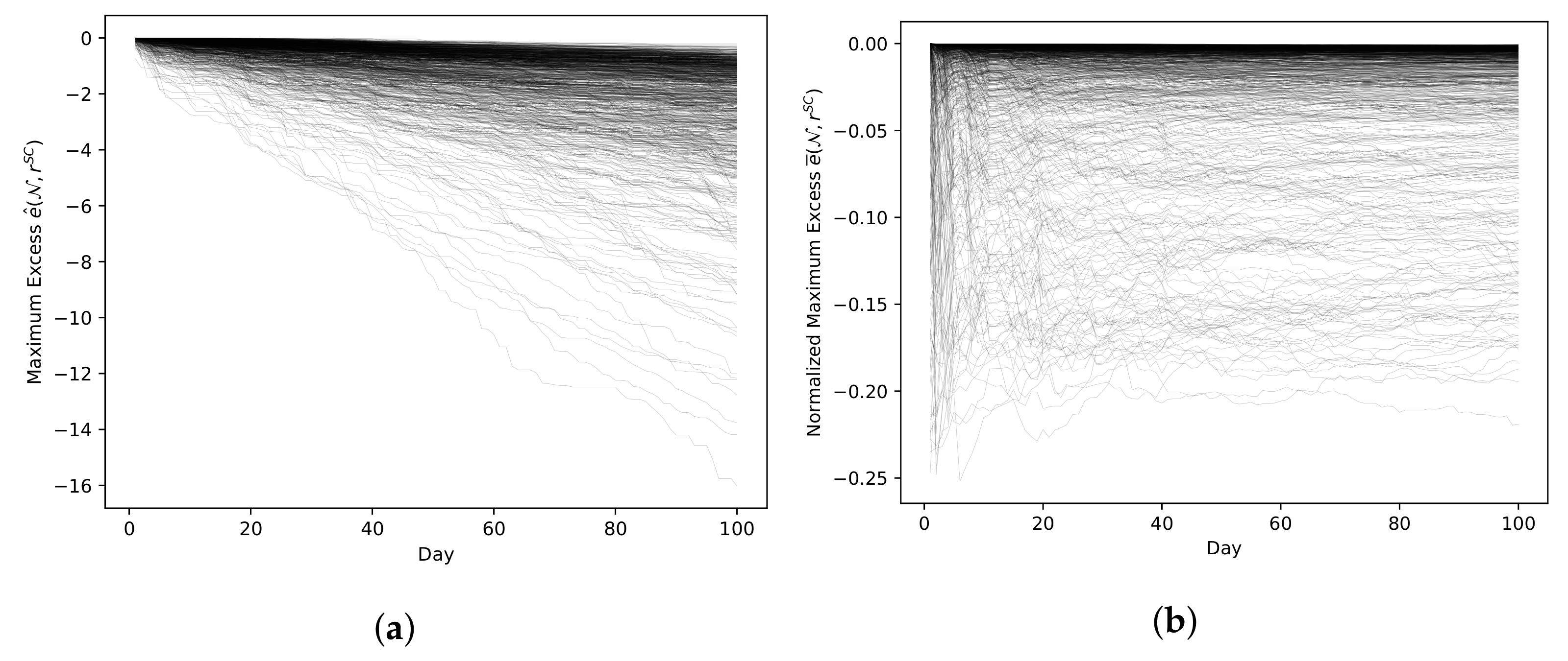
How stable is the Shapley value distribution in practice? Does it typically or even always yield an unstable distribution or not?

2.

If the Shapley value distribution is unstable, there is a sub-community that can gain a benefit from separating from the community. However, if this benefit is constant or even decreases over time, this might be not an issue in practice. How does the stability of the Shapley value progress over time?

3.

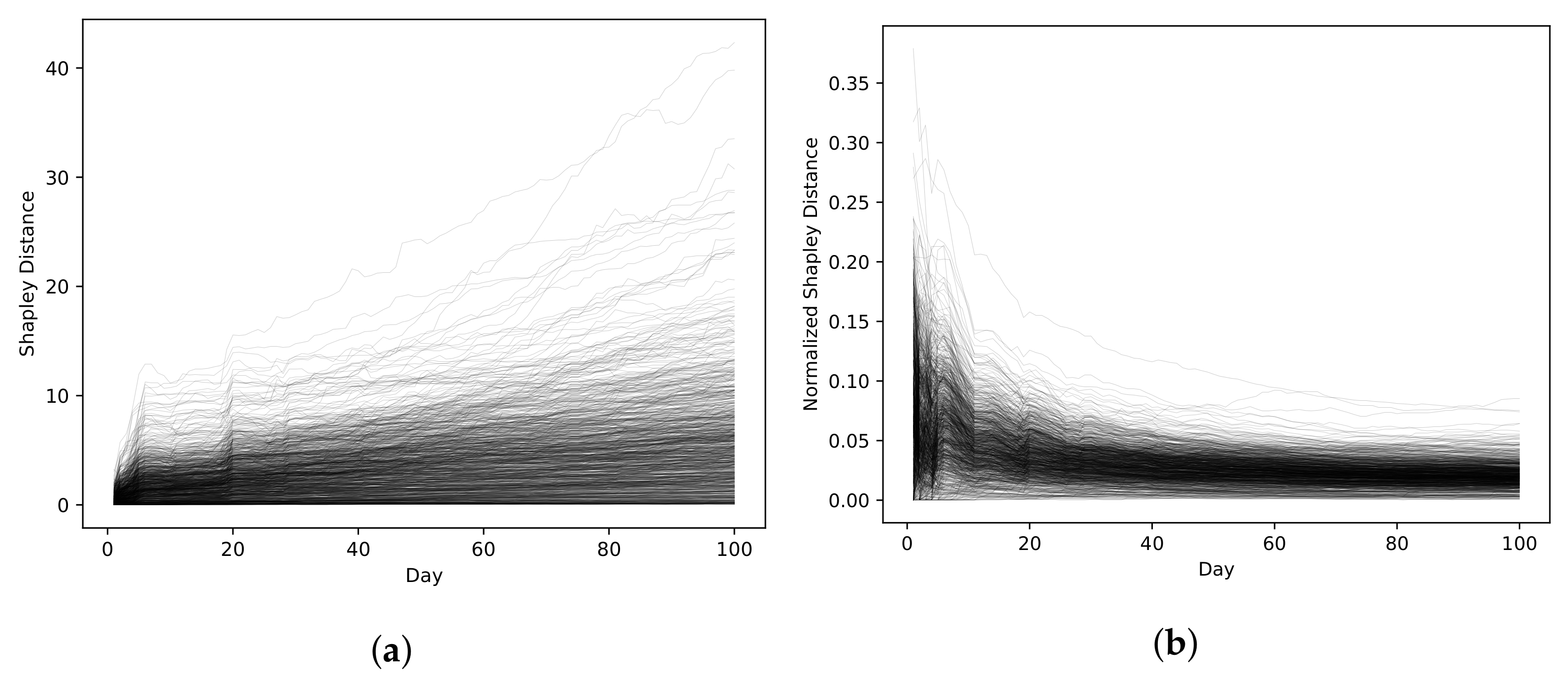
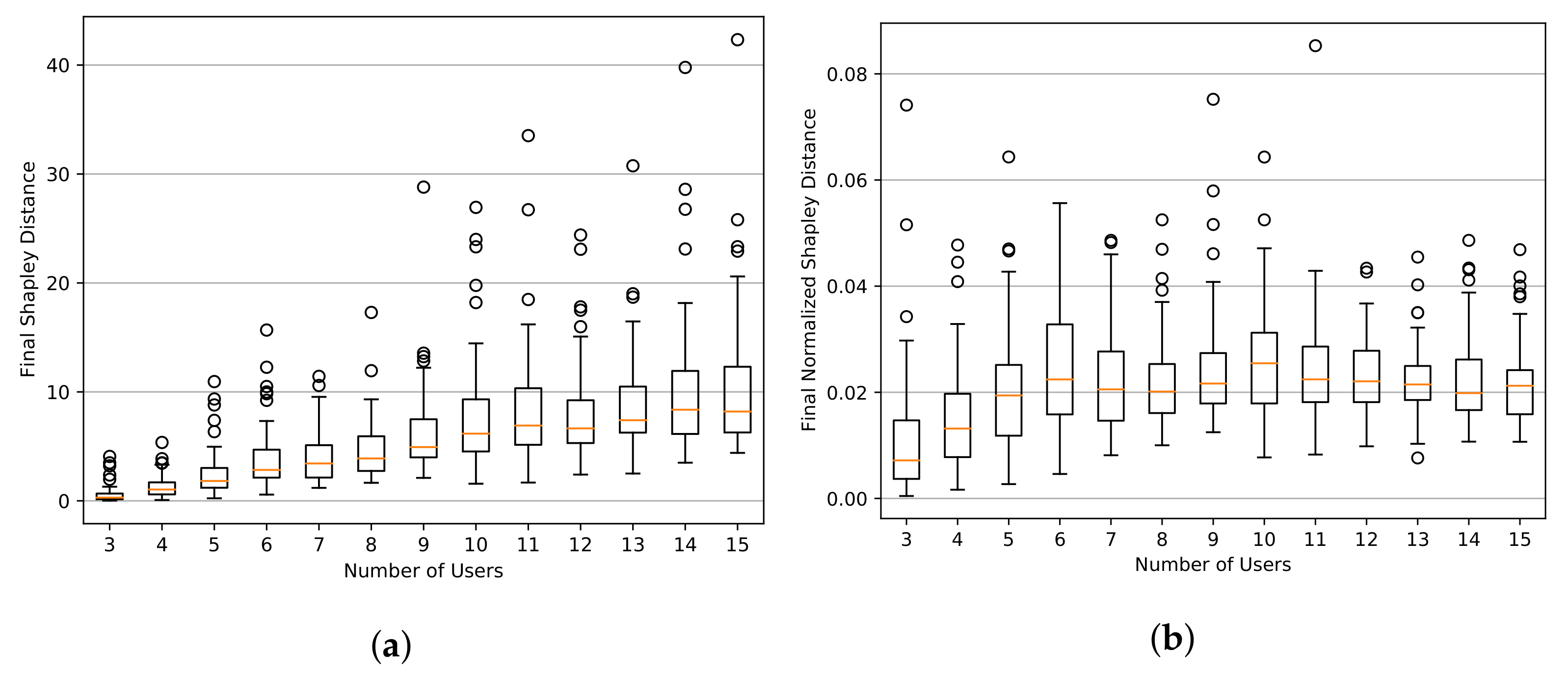
How unfair is the nucleolus in practice and how does its unfairness progress over time?

4.

Since the nucleolus is not additive, it does not guarantee maximum stability when applied over multiple billing periods. How does the nucleolus applied over multiple time periods perform in relation to the nucleolus applied to the full time frame?

5.

Similar to the nucleolus, the Shapley–core is not additive and not fully fair. How unfair is it and how do its unfairness and stability progress over time?

5. Experiments

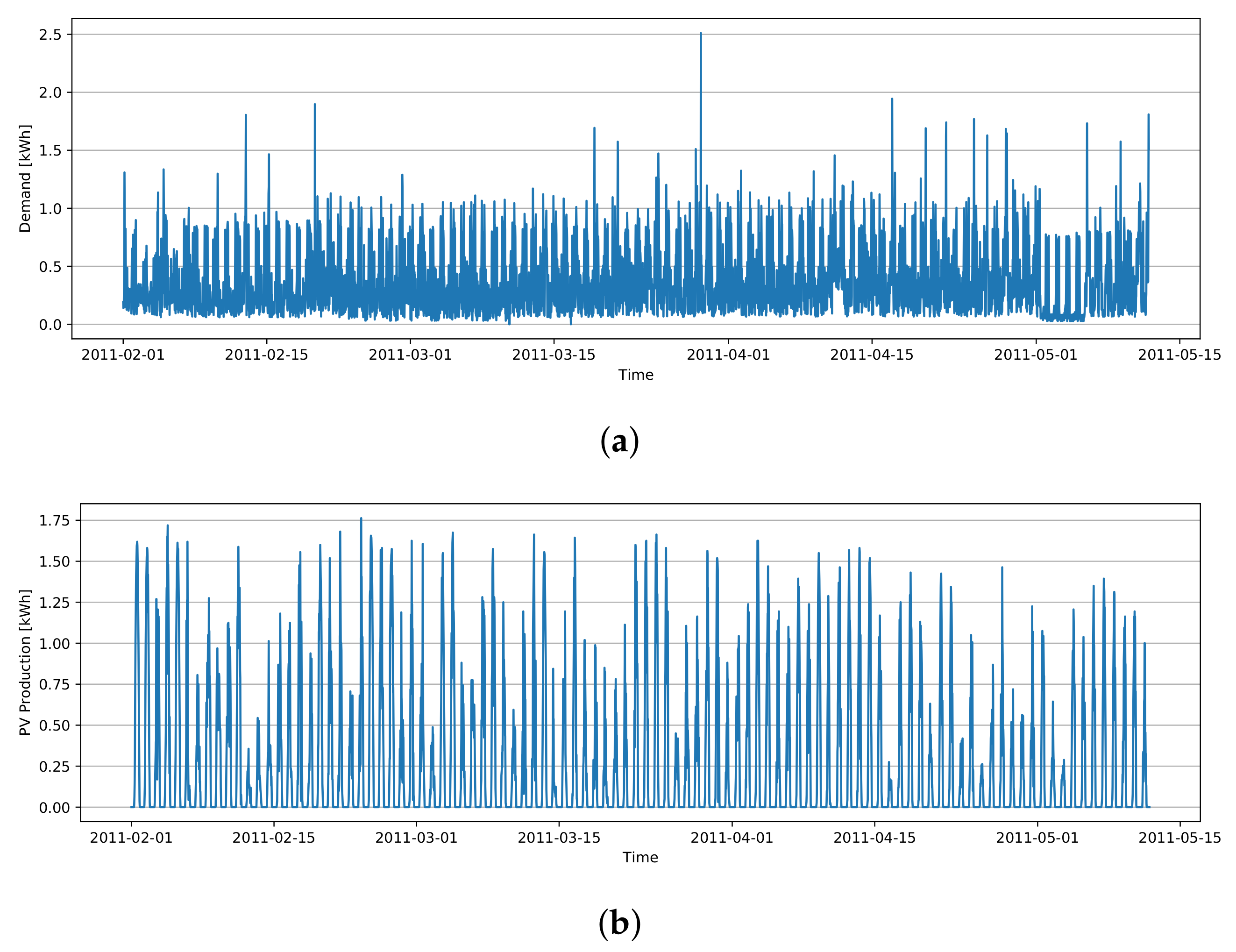
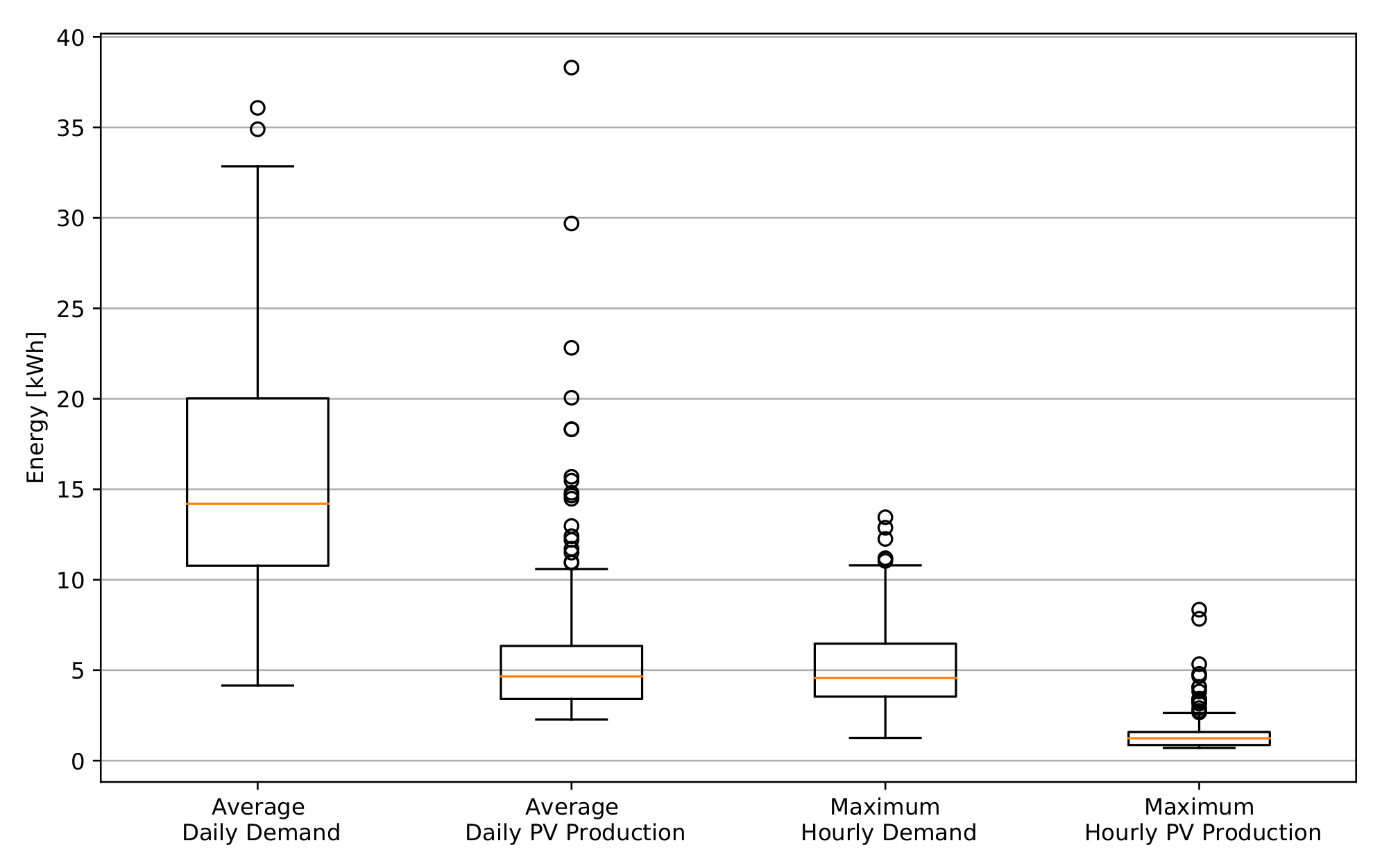
5.1. Use Case

In the experiments, we consider publicly available data of half-hourly energy demand and PV production of 300 Australian households equipped with PV systems [26]. We consider a time period of 100 days, starting with the first of February 2011. Figure 1 shows the half-hourly gross demand and PV production of one exemplary user during the considered time period.

A boxplot of the users’ average daily and maximum hourly demand and production in the considered time period is shown in Figure 2.

We assume a price of AUD 0.338 per kWh for energy bought from the grid [27] and a feed-in tariff of AUD 0.076 per kWh [28]. We executed 1000 trials. In each trial, an energy community $\mathcal{N}$ consisting of three to 15 randomly selected households is simulated. For each of the 100 considered days, the total benefit of the community gained on this day is distributed among the users in the community. For each user, the cumulative sum of his daily benefits is computed in order to compute his benefit gained between the start of the considered time period and the end of each day of the period. This is calculated with the SV, SC, and nucleolus benefit distribution schemes. Furthermore, for a comparison to the day-wise benefit distributions, the whole benefit of the community over all 100 days is distributed with the SC and nucleolus.

5.2. Experimental Results

5.2.1. Shapley Value

Figure 3a shows the progress of the maximum excess over the 100 days for the 1000 trials with Shapley value benefit distribution.

In 596 of the 1000 trials, the final maximum excess after 100 days is less than or equal to zero, meaning that the benefit distribution is stable. In the remaining 404 trials, the benefit distribution is unstable. However, as already stated, if the maximum excess does not increase over time, one can assume that the energy community would be stable in practice. Even if the maximum excess increases over time, it can be assumed that the sub-community with the maximum excess has no strong reason to separate from the community if their excess decreases in proportion to their benefit gained in the community. Figure 3b shows the progress of the maximum excess with the Shapley value normalized to the total benefit of the community $\overline{e}(\mathcal{N},r^{SV})=\frac{\widehat{e}(\mathcal{N},r^{SV})}{v\left(\mathcal{N}\right)}$. With help of a Mann–Kendall test [29,30], we determined whether there are statistically significant trends of the excesses and the normalized excesses between day 20 and day 100 with a significance level of 0.05. We do not consider the first 19 days in the test since, as one can see in Figure 3, there are high fluctuations in the first days.

Table 2. Numbers of unstable trials with increasing, decreasing, and no trend in the excess and normalized excess between day 20 and 100 with Shapley value benefit distribution.

Trend	Maximum Excess	Normalized Maximum Excess
Increasing	210	46
Decreasing	132	322
None	62	36

shows the results for the 404 unstable trials with positive final excess.

For 210 trials, the maximum excess is increasing, but in 322 trials, the normalized excess is decreasing. Thus, one can say that the Shapley value yielded a critically unstable benefit distribution in only 82 of the 1000 trials.

Figure 4 shows boxplots of the final excesses and normalized excesses after the 100 days subdivided by the number N of users in the energy community.

As one can see, the final excess tends to increase with an increasing number of users. Beginning with 10 users, the mean final excess is positive. Additionally, the final normalized excess tends to increase with an increasing number of users. Thus, one can say the larger the energy community, the more unstable the Shapley value becomes.

5.2.2. Nucleolus

Figure 5a shows the progress of the Shapley distance for the 1000 trials with nucleolus benefit distribution.

The Shapley distance of a certain benefit distribution is the Euclidean distance between the distribution and the corresponding benefit distribution with Shapley value. It can be interpreted as a measure of unfairness [24,31]. Figure 5a shows that the Shapley distance of the nucleolus distribution usually increases over time. However, this is not very surprising, since the total benefit increases and, thus, the norm of the Shapley value also increases. A better indicator for the unfairness is the Shapley distance normalized to the total benefit. The progress of the normalized Shapley distance in the 1000 trials can be seen in Figure 5b. Again, we used a Mann–Kendall test with a significance level of 0.05 to test the trends in the Shapley distances and normalized Shapley distances starting with day 20. The results are shown in

Table 3. Numbers of trials with increasing, decreasing, and no trend in the Shapley distance and normalized Shapley distance between day 20 and 100 with nucleolus.

Trend	Shapley Distance	Normalized Shapley Distance
Increasing	967	178
Decreasing	12	746
None	21	76

.

Although the Shapley distance increases in 967 trials, the normalized Shapley distance increases in only 178 trials. In 746 trials, the normalized Shapley distance even decreases. Hence, the nucleolus tends to become more fair over time. Figure 6 shows the distribution of the final Shapley distance and normalized Shapley distance with nucleolus per number of users.

While the absolute Shapley distance is rather independent of the number of users, the normalized Shapley distance decreases with an increasing number of users. As stated, the nucleolus is not additive. Thus, the day-wise computed nucleolus considered so far differs from the nucleolus computed over the full period. Figure 7 and Figure 8 show the distributions of the differences between the final excess and Shapley distance of the day-wise and full-period nucleolus separated by number of users.

The difference in the final excess is of course always positive, i.e., the stability of the day-wise nucleolus is weaker than that of the full-period nucleolus. The absolute difference is rather independent of the number of users, while the normalized excess decreases with a higher number of users. The difference in the Shapley distance has a tendency to decrease with an increasing number of users, and it is typically negative, meaning that the day-wise nucleolus is more fair than the full-period nucleolus.

5.2.3. Shapley–Core

Figure 9 shows the progress of the excess and normalized excess with Shapley–core benefit distribution.

Table 4. Number of trials with increasing, decreasing, and no trend in the excess and normalized excess between day 20 and 100 with Shapley–core benefit distribution.

Trend	Maximum Excess	Normalized Maximum Excess
Increasing	0	226
Decreasing	1000	641
None	0	133

shows the corresponding trends, and Figure 10 shows the distributions per number of users.

As can be seen, the excess increases, i.e., the stability of the benefit distribution becomes weaker, with an increasing number of users in the community. Analogously, Figure 11,

Table 5. Numbers of trials with increasing, decreasing, and no trend in the Shapley distance and normalized Shapley distance between day 20 and 100 with Shapley–core.

Trend	Shapley Distance	Normalized Shapley Distance
Increasing	935	128
Decreasing	36	816
None	29	56

, and Figure 12 show the progress, trends, and distributions per user of the Shapley distance. The normalized Shapley distance tends to decrease over time, but to increase with an increasing number of users.

Figure 13 shows the difference between the final maximum excess and normalized excess of the day-wise and full-period Shapley–core. The difference is typically negative, meaning that the day-wise Shapley–core is more stable than the full-period Shapley-core. However, there are also a few cases in which the day-wise Shapley–core is less stable.

Figure 14 shows the difference between the final Shapley distance and normalized Shapley distance of the day-wise and full-period Shapley–core. The distance is always positive, meaning that the day-wise Shapley–core is less fair than the full-period Shapley–core. This is not surprising, since it is typically also more stable. With an increasing number of users, the loss of fairness compared to the full-period Shapley–core tends to increase.

5.2.4. Comparison of Distributions

Figure 15 shows the mean final normalized excess and normalized Shapley distance per user number for the day-wise and full-period versions of nucleolus and Shapley–core and the Shapley value.

It can be seen that all distributions become less stable with an increasing number of users. The day-wise and full-period nucleolus become more fair with an increasing number of users, while the day-wise and full-period Shapley–core become less fair. Furthermore, the day-wise nucleolus and Shapley–core provide more and more similar results with an increasing number of users.

6. Conclusions

In simulation experiments, we investigated the stability and fairness of the Shapley value, the nucleolus and the Shapley–core. A total of 1000 cases of local energy communities were considered in the experiments. Based on the experimental results, we can answer the questions from Section 4 as follows:

1.

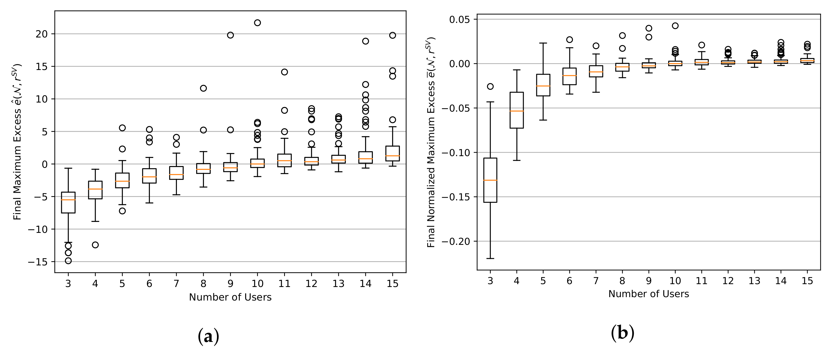
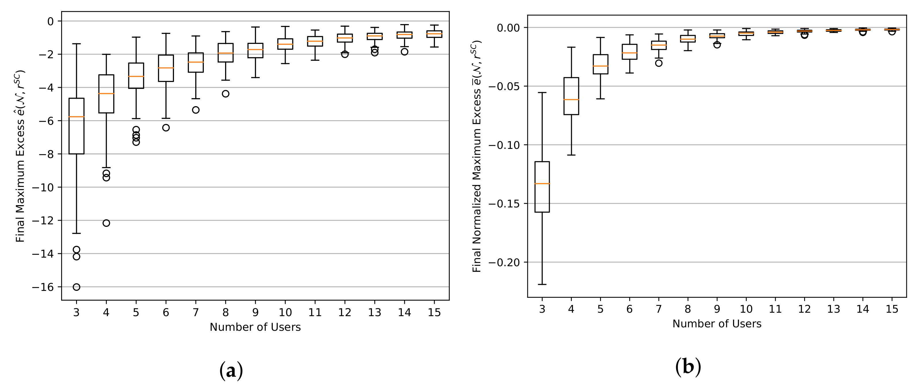
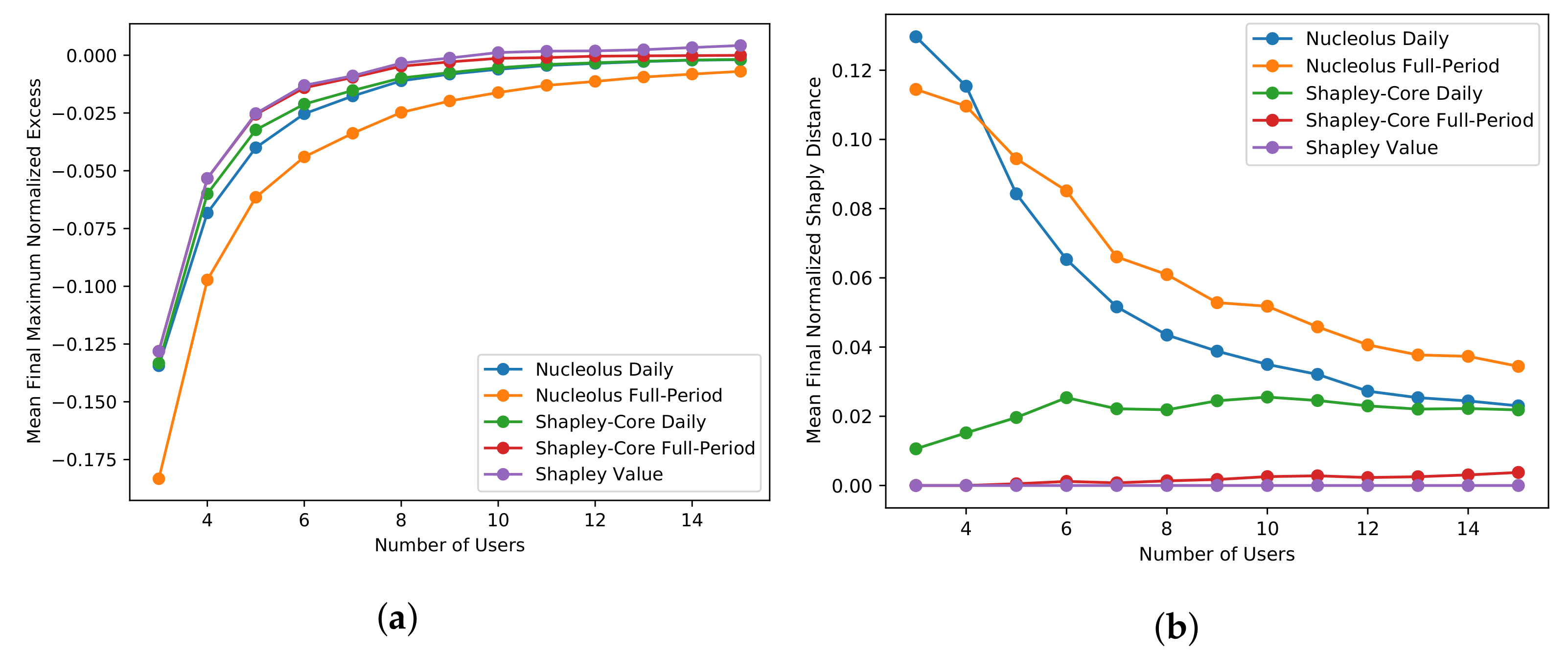
Q: How stable is the Shapley value distribution in practice? Does it typically or even always yield an unstable distribution or not?

A: The Shapley value does not necessarily yield an unstable distribution. In the experiments, it yielded a stable distribution in about 60% of the cases. However, with increasing size of the community, the Shapley value tends to become more unstable.

2.

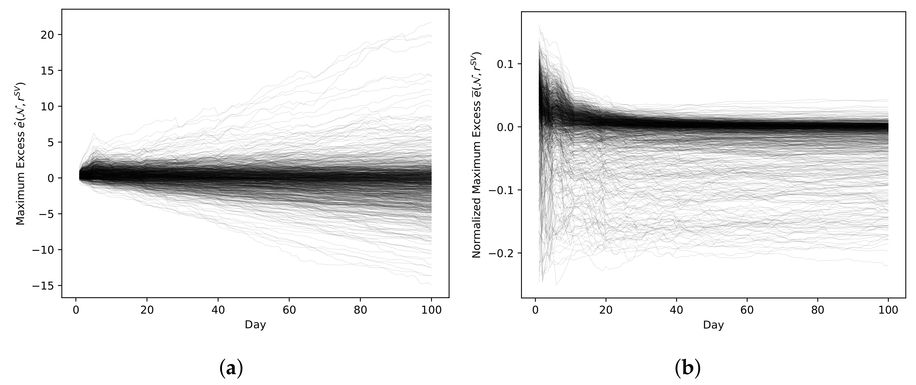
Q: If the Shapley value distribution is unstable, there is a sub-community that can gain a benefit from separating from the community. However, if this benefit is constant or even decreases over time, this might be not an issue in practice. How does the stability of the Shapley value progress over time?

A: In most of the cases where the Shapley value yielded an unstable distribution, the normalized maximum excess decreased in a statistically significantly way over time. In only about 8% of the considered cases, the Shapley value yielded an unstable distribution without a decreasing normalized maximum excess. Thus, in the remaining 92% of the cases, the Shapley value can be considered to be reasonably stable, at least from a practical point of view.

3.

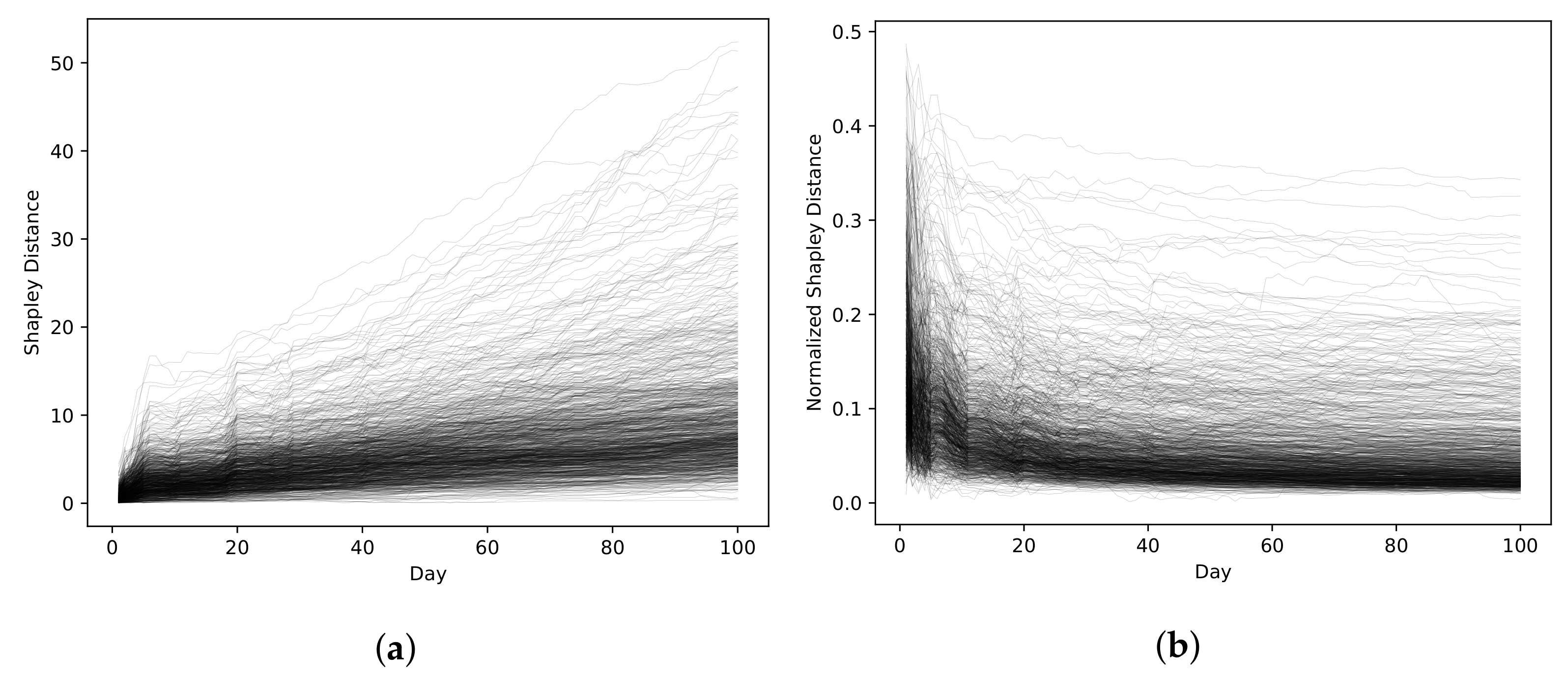
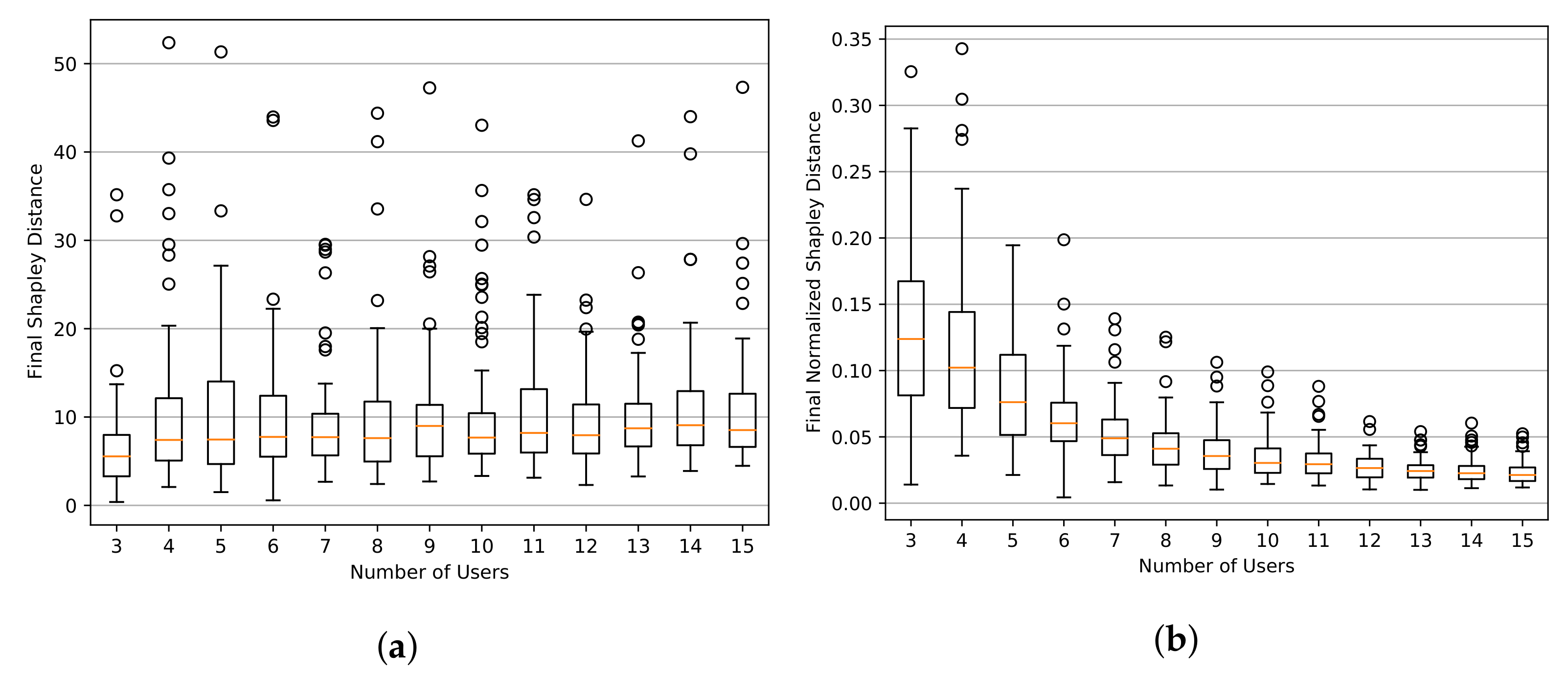
Q: How unfair is the nucleolus in practice and how does its unfairness progress over time?

A: The nucleolus tends to become more fair with increasing size of the community. While the maximum Shapley distance typically increases over time, the normalized Shapley distance decreased in a statistically significantly way in about 75% of the cases, meaning that in these cases, the nucleolus becomes more fair over time.

4.

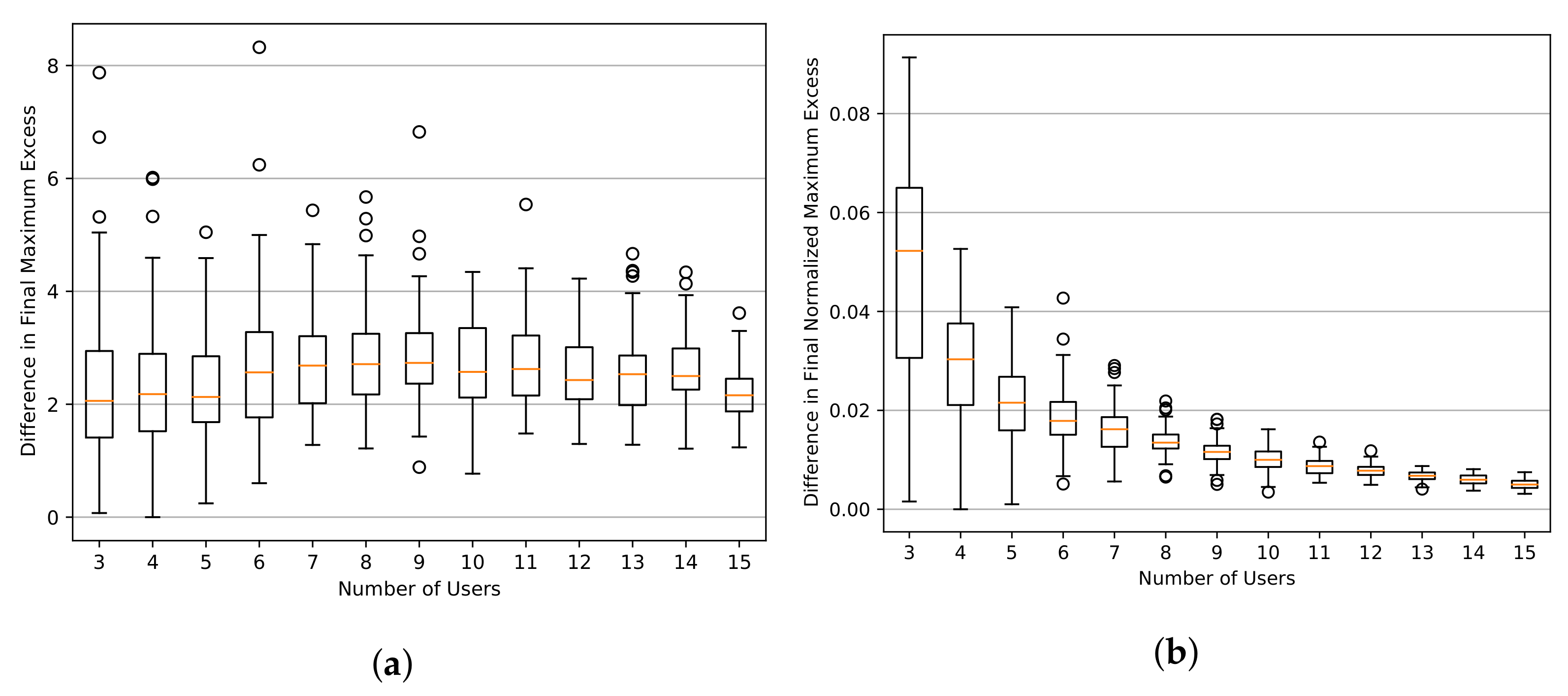
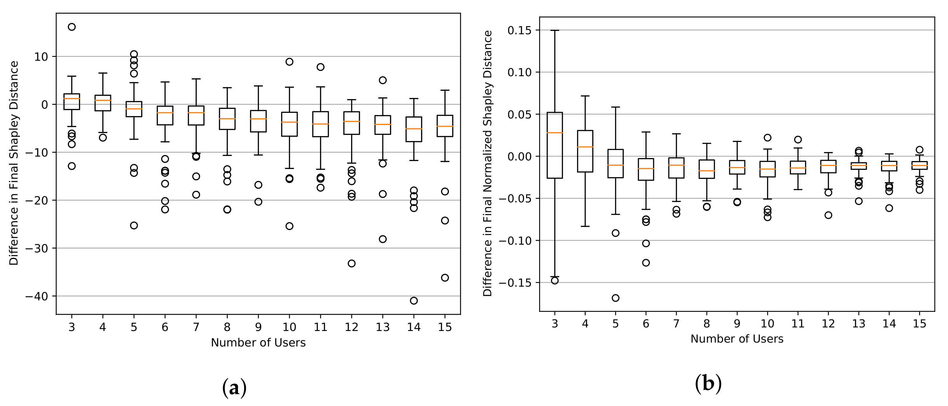
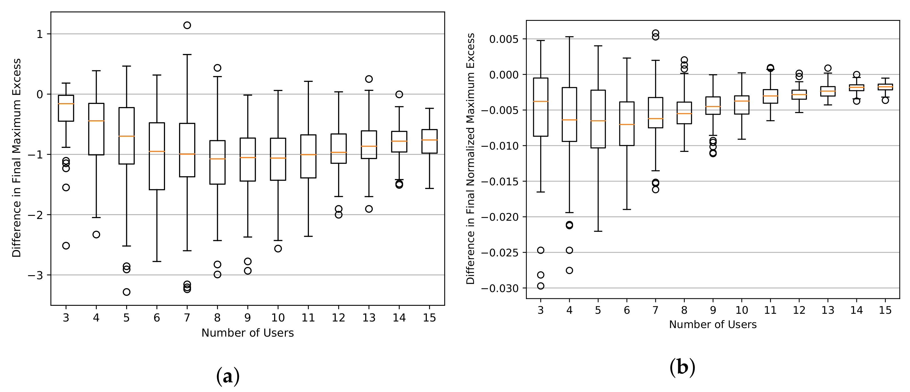
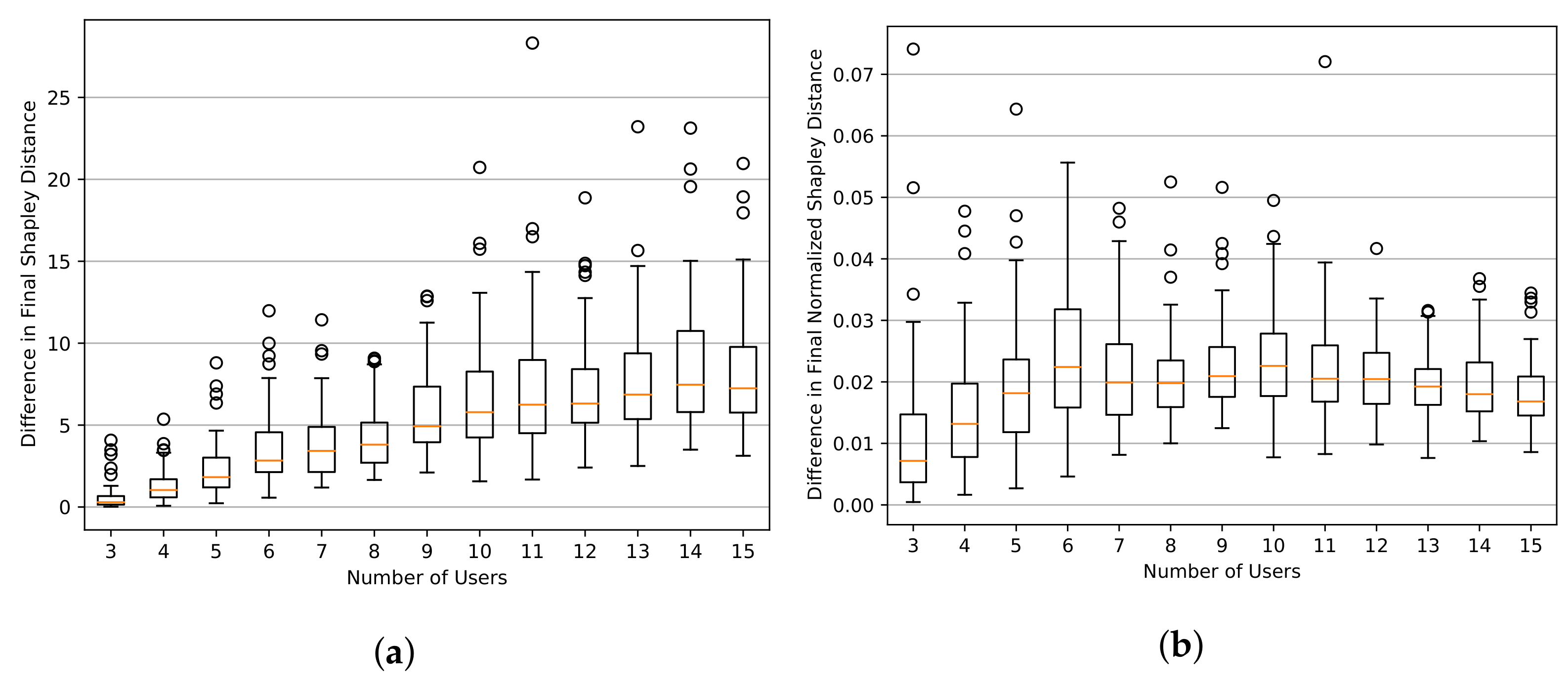
Q: Since the nucleolus is not additive, it does not guarantee maximum stability when applied over multiple billing periods. How does the nucleolus applied over multiple time periods perform in relation to the nucleolus applied to the full time frame?

A: In the experiments, the day-wise nucleolus yielded a higher maximum excess, i.e., a less stable distribution, than the full-period nucleolus in nearly all cases. For small communities, the day-wise nucleolus is typically also less fair. However, beginning with a certain community size, the day-wise nucleolus becomes more fair than the full-period nucleolus and the difference in stability in terms of normalized maximum excess decreases with increasing size of the community.

5.

Q: Similar to the nucleolus, the Shapley–core is not additive and not fully fair. How unfair is it and how do its unfairness and stability progress over time?

A: The day-wise Shapley–core is typically more stable but less fair than the full-period Shapley–core. With an increasing number of users, it becomes more and more similar to the day-wise nucleolus.

From this, we can conclude that for small communities, the Shapley value appears to be the best choice. However, with increasing community size, the risk that it yields a highly unstable distribution increases. By contrast, the nucleolus becomes more fair with increasing size of the community and, thus, it seems to be a better option than the Shapley value for larger communities. Alternatively, the Shapley–core could be employed, which behaves in a similar way to the nucleolus for large communities.

References

- Bauwens, T.; Schraven, D.; Drewing, E.; Radtke, J.; Holstenkamp, L.; Gotchev, B.; Yildiz, Ö. Conceptualizing community in energy systems: A systematic review of 183 definitions. Renew. Sustain. Energy Rev. 2022, 156, 111999. [Google Scholar] [CrossRef]
- Krug, M.; Di Nucci, M.R.; Caldera, M.; De Luca, E. Mainstreaming Community Energy: Is the Renewable Energy Directive a Driver for Renewable Energy Communities in Germany and Italy? Sustainability 2022, 14, 7181. [Google Scholar] [CrossRef]
- Energy Communities Repository. Available online: https://energy-communities-repository.ec.europa.eu/about_en (accessed on 23 January 2023).
- Zhang, C.; Wu, J.; Long, C.; Cheng, M. Review of Existing Peer-to-Peer Energy Trading Projects. Energy Procedia 2017, 105, 2563–2568. [Google Scholar] [CrossRef]
- Rahmani, S.; Murayama, T.; Nishikizawa, S. Review of community renewable energy projects: The driving factors and their continuation in the upscaling process. IOP Conf. Ser. Earth Environ. Sci. 2020, 592, 012033. [Google Scholar] [CrossRef]
- Mengelkamp, E.; Staudt, P.; Garttner, J.; Weinhardt, C. Trading on local energy markets: A comparison of market designs and bidding strategies. In Proceedings of the 2017 14th International Conference on the European Energy Market (EEM), Dresden, Germany, 6–9 June 2017; pp. 1–6. [Google Scholar] [CrossRef]
- Lezama, F.; Soares, J.; Faia, R.; Vale, Z.; Kilkki, O.; Repo, S.; Segerstam, J. Bidding in local electricity markets with cascading wholesale market integration. Int. J. Electr. Power Energy Syst. 2021, 131, 107045. [Google Scholar] [CrossRef]
- Garcìa-Muñoz, F.; Teng, F.; Junyent-Ferré, A.; Díaz-González, F.; Corchero, C. Stochastic energy community trading model for day-ahead and intraday coordination when offering DER’s reactive power as ancillary services. Sustain. Energy Grids Netw. 2022, 32, 100951. [Google Scholar] [CrossRef]
- Etukudor, C.; Couraud, B.; Robu, V.; Früh, W.G.; Flynn, D.; Okereke, C. Automated Negotiation for Peer-to-Peer Electricity Trading in Local Energy Markets. Energies 2020, 13, 920. [Google Scholar] [CrossRef]
- Capper, T.; Gorbatcheva, A.; Mustafa, M.A.; Bahloul, M.; Schwidtal, J.M.; Chitchyan, R.; Andoni, M.; Robu, V.; Montakhabi, M.; Scott, I.J.; et al. Peer-to-peer, community self-consumption, and transactive energy: A systematic literature review of local energy market models. Renew. Sustain. Energy Rev. 2022, 162, 112403. [Google Scholar] [CrossRef]
- Grzanić, M.; Morales, J.M.; Pineda, S.; Capuder, T. Electricity Cost-Sharing in Energy Communities Under Dynamic Pricing and Uncertainty. IEEE Access 2021, 9, 30225–30241. [Google Scholar] [CrossRef]
- Fioriti, D.; Frangioni, A.; Poli, D. Optimal sizing of energy communities with fair revenue sharing and exit clauses: Value, role and business model of aggregators and users. Appl. Energy 2021, 299, 117328. [Google Scholar] [CrossRef]
- Pires Klein, L.; Krivoglazova, A.; Matos, L.; Landeck, J.; de Azevedo, M. A Novel Peer-To-Peer Energy Sharing Business Model for the Portuguese Energy Market. Energies 2020, 13, 125. [Google Scholar] [CrossRef]
- Foroozandeh, Z.; Limmer, S.; Lezama, F.; Faia, R.; Ramos, S.; Soares, J. A MBNLP Method for Centralized Energy Pricing and Scheduling in Local Energy Community. In Proceedings of the IEEE PES Generation, Transmission and Distribution Conference & Exposition Latin America 2022, La Paz, Bolivia, 20–22 October 2022. [Google Scholar]
- Norbu, S.; Couraud, B.; Robu, V.; Andoni, M.; Flynn, D. Modelling the redistribution of benefits from joint investments in community energy projects. Appl. Energy 2021, 287, 116575. [Google Scholar] [CrossRef]
- Long, C.; Wu, J.; Zhang, C.; Thomas, L.; Cheng, M.; Jenkins, N. Peer-to-peer energy trading in a community microgrid. In Proceedings of the 2017 IEEE Power & Energy Society General Meeting, Chicago, IL, USA, 16–20 July 2017; pp. 1–5. [Google Scholar] [CrossRef]
- Chau, S.C.K.; Xu, J.; Bow, W.; Elbassioni, K. Peer-to-Peer Energy Sharing: Effective Cost-Sharing Mechanisms and Social Efficiency. In Proceedings of the Tenth ACM International Conference on Future Energy Systems. Association for Computing Machinery, Phoenix, AZ, USA, 25–28 June 2019; pp. 215–225. [Google Scholar] [CrossRef]
- Gjorgievski, V.Z.; Cundeva, S.; Markovska, N.; Georghiou, G.E. Virtual net-billing: A fair energy sharing method for collective self-consumption. Energy 2022, 254, 124246. [Google Scholar] [CrossRef]
- Shapley, L.S. A Value for n-Person Games. In Contributions to the Theory of Games (AM-28); Kuhn, H.W., Tucker, A.W., Eds.; Princeton University Press: Princeton, NJ, USA, 1953; Volume II, pp. 307–318. [Google Scholar] [CrossRef]
- Schmeidler, D. The Nucleolus of a Characteristic Function Game. SIAM J. Appl. Math. 1969, 17, 1163–1170. [Google Scholar] [CrossRef]
- Abada, I.; Ehrenmann, A.; Lambin, X. On the Viability of Energy Communities; Technical Report; Energy Policy Research Group, University of Cambridge: Cambridge, UK, 2017. [Google Scholar]
- Long, C.; Zhou, Y.; Wu, J. A game theoretic approach for peer to peer energy trading. Energy Procedia 2019, 159, 454–459. [Google Scholar] [CrossRef]
- Li, J.; Ye, Y.; Papadaskalopoulos, D.; Strbac, G. Computationally Efficient Pricing and Benefit Distribution Mechanisms for Incentivizing Stable Peer-to-Peer Energy Trading. IEEE Internet Things J. 2021, 8, 734–749. [Google Scholar] [CrossRef]
- Aguiar, V.H.; Pongou, R.; Serrano, R.; Tondji, J.B. An index of unfairness. In Handbook of the Shapley Value; Chapman and Hall/CRC: New York, NY, USA, 2019; pp. 31–48. [Google Scholar]
- Van den Brink, R. An axiomatization of the Shapley value using a fairness property. Int. J. Game Theory 2002, 30, 309–319. [Google Scholar] [CrossRef]
- Ratnam, E.L.; Weller, S.R.; Kellett, C.M.; Murray, A.T. Residential load and rooftop PV generation: An Australian distribution network dataset. Int. J. Sustain. Energy 2017, 36, 787–806. [Google Scholar] [CrossRef]
- Cost of Electricity in Australia—How Are We Doing in 2020? Available online: https://www.leadingedgeenergy.com.au/news/cost-of-electricity-in-australia-in-2020/ (accessed on 23 January 2023).
- EnergyAustralia Feed-in Tariff NSW. Available online: https://www.energyaustralia.com.au/home/solar/feed-in-tariffs (accessed on 23 January 2023).
- Mann, H.B. Nonparametric Tests Against Trend. Econometrica 1945, 13, 245–259. [Google Scholar] [CrossRef]
- Kendall, M.G. Rank Correlation Methods; Griffin: London, UK, 1975. [Google Scholar]
- Aguiar, V.H.; Pongou, R.; Tondji, J.B. A non-parametric approach to testing the axioms of the Shapley value with limited data. Games Econ. Behav. 2018, 111, 41–63. [Google Scholar] [CrossRef]