Analysis of the Influence of Nodal Reactive Powers on Voltages in a Power System

Abstract

The paper deals with finding power system nodes where reactive powers have the greatest influence on system voltages. The problem to be solved is important in reactive power planning. Its proper solution indicates in which nodes new sources of reactive power should be installed in order to achieve the assumed goals in the aforementioned planning. So far, the problem formulated earlier has not been satisfactorily resolved. The paper presents an original method, which, based on the entire history of the system operation states, allows a solution to the problem mentioned above to be found. The proposed method assumes the use of measurement data of nodal-voltage magnitudes and nodal reactive power. Correlational relationships between the above-mentioned quantities are investigated. The paper shows that the considered correlational relationships are not linear. In this situation, Kendall’s rank correlation coefficient is used to evaluate the strength of these correlational relationships. Analysis of the strongest relationships allows us to identify those nodal reactive powers that have the greatest influence on the voltages in the power system. The results of the analysis are the basis for determining the location of additional reactive power sources in the power system, which is very essential in reactive power planning. The proposed method is relatively easy to implement and does not require complicated calculations. The paper additionally shows that failure to use the entire spectrum of representative system states when solving the problem under consideration can adversely affect the result.

1. Introduction

Voltages are essential quantities distinguished in a Power System (PS). They are taken into account in different PS analyses. They are also included in solving various power-system problems. The paper focuses on the nodal voltages in PS, and more specifically on the relationships between nodal-voltage magnitudes and nodal reactive powers. Knowledge of those relationships is particularly important in relation to analyses related to reactive-power planning. An important problem that arises here, and for the solution of which the aforementioned knowledge is essential, is the problem of identifying candidate nodes for the location of additional reactive-power sources.

There are many papers devoted to reactive power planning. The goal of reactive-power planning is to find the most favorable locations for additional reactive power sources and the most favorable parameters for them from the point of view of an assumed criterion. Voltages are taken into account when constructing the reactive-power-planning objective function. They are also taken into consideration when determining candidate nodes for the location of additional reactive power sources in PS.

Taking into account the reactive-power-planning objective function, it can be seen that it can directly refer to the deviations of nodal-voltage magnitudes from the selected values. For example, this is the case in [1,2,3]. The situation is slightly different, for example, in [4,5], where for the purposes of reactive-power planning, one of the considered objective functions is defined as the sum of the absolute values of differences in voltage magnitudes (in pu) in particular nodes and the value 1 pu.

A modification of the approach used in [1,2,3,4,5] is one presented in [6]. In that paper, one of the considered objective functions is defined using the mean value of the voltage deviations for the key nodes in PS in a steady state at the time t_f relative to the instant of time before the fault. The time t_f is after the fault occurred. All distinguished faults are taken into account when calculating the mentioned mean value.

It is easy to see that the stronger the relationships between a given nodal reactive power and nodal voltages in PS, the greater the influence of the considered nodal reactive power on the value of the objective function taken into account in the reactive-power planning process.

Particularly in real-world large-scale PSs, finding the best locations for additional reactive-power sources and the sizes of these sources at the same time is a difficult task. Thus, instead of reviewing all possible locations of additional reactive power sources (as it is in [5]), the candidate nodes for the location of these additional sources are first found, and only then are their sizes determined. In this situation, the indices characterizing nodal voltages can be used for finding nodes for the location of additional reactive-power sources.

A simple solution is used in [2], where it is stated that if the voltage deviation index for a node, which can be presented as the difference in reference voltage magnitude and the nodal-voltage magnitude, is large enough, then the considered node is a candidate for the placement of a capacitor.

In [7], to determine candidate nodes for the location of additional reactive-power sources, for each node, the sum of changes in all nodal-voltage magnitudes in PS is calculated when the nodal reactive power of this node increases by a certain amount. Load nodes with the large mentioned sums are good candidates for additional reactive-power source sites.

In [8], it is ascertained that for a candidate node from the viewpoint of the location of an additional reactive-power source (compensator), the V-Q sensitivity index should be sufficiently large. That index is defined as the mean value of derivatives of nodal-voltage magnitudes in PS, with respect to reactive power at the considered node. The index defined in the paper characterizes the influence of the nodal reactive power, at the node under consideration, on the voltages in PS.

More complicated calculations of the index qualifying nodes to locate additional reactive power sources can be found in [9] and earlier in [10]. The index is calculated for each node in PS. For the k-th node, the index is the square root of the mean value of the squared differences, each of which is a difference of 1 pu and the RMS of the nodal voltage in the considered node under the following assumptions: (i) the mentioned differences are calculated for each node in PS; and (ii) nodal voltages in these differences are determined, when a capacitor with a size equal to 25% of the total system capacity is connected to the k-th node. The smallest values of the index qualify the appropriate nodes for the location of the capacitors.

Another method of finding candidate nodes for the location of additional reactive-power sources is the modal analysis of the matrix linking changes in nodal reactive powers with changes in nodal-voltage magnitudes [11]. This matrix is obtained from the Jacobi matrix appearing in the equation linking changes in nodal active and reactive powers with changes in arguments and magnitudes of nodal voltages. The mentioned equation is used in the Newton–Raphson method. The eigenvalues of the considered matrix correspond to changes in nodal-voltage magnitudes and nodal reactive powers, which are used to find candidate nodes for the location of additional reactive-power sources. The smaller the eigenvalue of the matrix, the more suitable the node is for locating additional reactive-power sources.

1.1. Critical Evaluation of the Existing Solutions of the Considered Problem

When formulating the reactive-power planning task, it is assumed that nodal reactive powers are among the independent variables. The solution of the reactive-power planning task allows us to indicate those of the nodal reactive powers that have a significant influence on the objective function. This means that the objective function, and in particular, the nodal-voltage magnitudes being in the objective function, are sensitive to the found reactive powers. The considered fact also means that the nodes, at which there are the above-mentioned reactive powers, are candidate nodes for the location of additional reactive-power sources. It should be added that the extremization of the objective function (it is often a minimization of this function) should be made from the point of view of all possible operating states of PS or, at least, from the point of view of the representative states of this system. That is a serious problem in the investigation of reactive-power planning, as can be seen in the earlier-cited papers (in the previous part of this section), which do not even address this problem. Moreover, the previously-presented methods for selecting candidate nodes for the location of additional reactive-power sources do not ensure satisfying the given condition. Those methods tell us how to select the mentioned nodes for a specific operating state of PS. However, it may turn out that for a different operating state of PS, other nodes are candidates for the location of additional reactive-power sources. From the point of view of reactive-power planning, it is not possible to indicate different sets of nodes for the location of additional reactive-power sources for different PS operating states. The reactive-power planning task is an investment task, which means that one set of nodes for locating additional reactive-power sources is to be pointed out for all possible PS operating states.

It should be added that many of the methods of determining the set of candidate nodes for the location of additional reactive-power sources require a large computational effort. This applies to the methods described in [7,8,9,10], and in particular, the method described in [11].

1.2. Contributions

Based on the existing papers, the following goal is formulated: To develop an effective and computationally efficient method for finding candidate nodes for the location of additional reactive-power sources, taking into account all possible states of PS and the knowledge of the relationships between nodal-voltage magnitudes and nodal reactive powers in PS. As a result of the conducted investigations, the following original results were obtained:

• Theoretical considerations showed that the relationships between the nodal-voltage magnitudes in PS and the nodal reactive powers are non-linear.
• The approach to evaluating the relationships between the nodal-voltage magnitudes and the nodal reactive powers for all PS operating states that are characterized by the available data.
• Development of a method for finding candidate nodes for the location of additional reactive-power sources, taking into account all PS operating states for which data are available.
• The use of the proposed method for a specific PS.
• Using the Monte Carlo method demonstrates that the results of searching for candidate nodes for the location of additional reactive-power sources, determined on the basis of a subset of all PS operating states, may differ from the results of searching for these nodes on the basis of all PS operating states.
• Analysis of the influence of the level of statistical significance on the results of the proposed method for determining the set of candidate nodes for the location of additional reactive-power sources.

In general, the carried-out investigation uses a statistical approach. The study of correlational relationships between the nodal reactive powers and the nodal-voltage magnitudes is used. Therefore, further down in the paper, in Section 2, general characteristics of the used statistical approach are presented. In Section 3, different measures of correlation are described, and in Section 4, the selection of correlation measure to be used in the planned investigation is considered. In Section 5, basic concepts related to the used correlational relationships are introduced. Those concepts are used in the proposed method, which is presented in Section 6. Section 7 is devoted to the results of the calculations, which are to (i) illustrate the various stages of applying the proposed method; and (ii) show the results of searching for the location of additional reactive power sources, when only a certain part of the whole operating-state space of PS is considered. A discussion of the results of the conducted calculations is in Section 8. Section 9 contains the conclusions.

2. General Characteristics of the Used Statistical Approach

The loads in PS are constantly changing and therefore the generation of electrical energy is also changing. The mentioned changes are random. Thus, statistical methods can be used to analyze randomly changing quantities in PS.

In order to solve the problem considered in the paper, it is necessary to analyze the relationships between the nodal reactive powers and the nodal-voltage magnitudes over a longer period of time. The statistical approach taken into account leads to the analysis of Correlational Relationships (CRs) between considered quantities. CR simply says that two considered variables perform in a synchronized manner [12]. The evaluation of the extent to which that takes place [13,14] is the subject of the conducted analysis. The results of such an analysis are the basis for indicating nodal reactive powers that have the strongest influence on nodal-voltage magnitudes. Nodes with such reactive powers are treated as candidate nodes for the location of additional reactive power sources.

It should be noted that the investigation of CRs for the purposes of analyses related to PS has already been conducted in other papers. Such papers are [15,16,17,18,19,20,21]. In [15], a relationship between the injected power and the voltage quality at the node, in which installation of a new source is considered, is investigated with the use of the Pearson correlation coefficient. The correlation approach with the use of the same correlation coefficient to solving the problem of grouping nodes in PS is presented in [16]. Another problem solved with the use of that approach is the identification of a low-frequency oscillation source [17]. Whereas, in [18], the identification of the sources of power quality disturbances is considered.

The correlation approach, assuming a partial correlation study, was also proposed to identify the disturbance source affecting power quality, which is described in [19].

The correlation analysis using a different correlation coefficient than in the previously cited papers, i.e., using Spearman’s rank correlation coefficient, is used to solve the problems considered in [20,21]. Paper [20] describes an investigation of influence of the nodal reactive powers on power flow in PS. Paper [21] deals with the propagation of voltage-RMS-value deviations in PS.

None of the mentioned papers [15,16,17,18,19,20,21] uses correlation analysis to investigate the influence of the nodal reactive powers on the nodal-voltage magnitudes, which is the case in this paper. Unlike papers [15,16,17,18,19], this paper analyzes the nature of the relationships between the distinguished quantities. As a result of this analysis, it is possible to properly select the correlation coefficient used in the investigations of CRs. The mentioned analysis concluded that Kendal’s rank correlation coefficient should be used in the described investigations.

3. Measures of Correlation

The strength of CR can be assessed using one of the following measures: (i) Pearson product-moment correlation coefficient (Pearson’s correlation coefficient), (ii) Spearman’s rank correlation coefficient, or (iii) Kendall’s rank correlation coefficient [13,14]. Pearson’s Correlation Coefficient (PCC) is used when the relationship between considered quantities X and Y is linear. When that relationship is not linear, Spearman’s Rank Correlation Coefficient (SRCC) or Kendall’s Rank Correlation Coefficient (KRCC) is an appropriate measure of the strength of CR. In [13], the cases are shown, where the evidence of association between values of X and Y provided by KRCC is stronger than that provided by SRCC. KRCC is easier to compute and more importantly in practice because the assumption about equally spaced values of X is not needed here.

When measurement data of variables X and Y are available, PCC can be calculated as follows [13]:

$$r_{\mathrm{P}}=\frac{{{\displaystyle \sum }}_{i=1}^m\left(X_i-\overline{X}\right)·\left(Y_i-\overline{Y}\right)}{\sqrt{{{\displaystyle \sum }}_{i=1}^m{\left(X_i-\overline{X}\right)}^2} \sqrt{{{\displaystyle \sum }}_{i=1}^m{\left(Y_i-\overline{Y}\right)}^2}},$$

(1)

where

$$\overline{X}=m^{-1}{{\displaystyle \sum }}_{i=1}^m{X}_i,$$

(2)

$$\overline{Y}=m^{-1}{{\displaystyle \sum }}_{i=1}^m{Y}_i,$$

(3)

m—a number of measurement data; X_i, Y_i i ∈{1, 2, …, m}—i-th items of measurement data of variables X and Y, respectively.

If the variables X and Y are described by a bivariate normal distribution, then the following variable

$$t=r_{\mathrm{P}}\sqrt{\frac{m-2}{1-r_{\mathrm{P}}^2}},$$

(4)

has a Student’s t-distribution with degrees of freedom m − 2 in the null case, i.e., when the variables X and Y are independent. That statement is approximately valid, even if values of the variables X and Y cannot be characterized by normal distributions, when m is sufficiently large. Knowing the properties of the variable t can be used to test the hypothesis that the variables X and Y are not statistically dependent. Thus, in this test, H₀ is the hypothesis that variables X and Y are statistically independent, and H_a is the hypothesis that variables X and Y are statistically dependent.

The definition of SRCC (r_S) is as follows [13]:

$$r_{\mathrm{S}}=r_{\mathrm{P}}\left(\mathrm{rg}X,\mathrm{rg}Y\right)=\mathrm{cov}\left(\mathrm{rg}X,\mathrm{rg}Y\right)/\left({\sigma }_{\mathrm{rg}X}{\sigma }_{\mathrm{rg}Y}\right),$$

(5)

where rgX, rgY—ranks of variables X and Y, respectively.

The test of significance of r_S uses the statistic t defined by Equation (4), when r_P is replaced by r_S and pairs (X_i, Y_i) i ∈{1, 2, …, m} are independent. The assumption of normality of the distributions of X and Y is not required.

When m tends to infinity, in the test of significance of r_S a statistic defined as follows is used

$$z=r_{\mathrm{S}}\sqrt{m-2}.$$

(6)

Assuming the statistical independence of variables X and Y, the z-statistic distribution tends to the standard normal distribution as m tends to infinity.

KRCC (t_k) can be calculated using the formula [13]:

$$t_{\mathrm{k}}=\left(c-d\right)/\left(c+d\right),$$

(7)

where c, d—the numbers of concordant and discordant pairs of observations (X_i, Y_i) i ∈{1, 2, …, m} in the sample, respectively.

The pairs (X_j, Y_j) and (X_k, Y_k) are concordant if X_j < X_k and Y_j < Y_k or if X_j > X_k and Y_j > Y_k (i.e., (X_j − X_k)(Y_j − Y_k) > 0) and discordant if X_j < X_k and Y_j > Y_k or if X_j > X_k and Y_j < Y_k (i.e., (X_j − X_k)(Y_j − Y_k) < 0). There are m(m-1)/2 distinct pairs of observations in the sample.

In the significance test of t_k, the following statistic is used:

$$z=\frac{3\left(c-d\right)}{\sqrt{m\left(m-1\right)\left(2m+5\right)/2}} .$$

(8)

Under the assumption that variables X and Y are statistically independent, the statistic z is approximately distributed as a standard normal.

4. Selection of the Correlation Measure in the Considered Investigation

The correct selection of the correlation measure requires an analysis of the relationship between the quantities whose correlation is investigated. Therefore, an analysis of the relationships between the nodal reactive powers and the nodal-voltages magnitudes in PS is carried out.

The following matrix equation can be given for PS, linking the nodal powers with the nodal voltages

$$P-\mathrm{j}Q={\overline{V}}_{\mathit{D}}^{*} \overline{Y} \overline{V},$$

(9)

where P, Q—vectors of nodal active powers and nodal reactive powers, respectively; ${\overline{V}}_{\mathit{D}}^{}$—a diagonal matrix of complex nodal voltages; $\overline{Y}$—a complex PS admittance matrix; $\overline{V}$—a vector of complex nodal voltages; *—a symbol for the conjugate of complex quantities; j—the unit imaginary number.

For node j j ∈ {1, 2, …, n}, where n—a number of nodes in PS, we can write

$$P_j-\mathrm{j}{Q}_j={\overline{V}}_j^{*}{{\displaystyle \sum }}_{i=1}^n{\overline{Y}}_{ji}^{}{\overline{V}}_i^{},$$

(10)

where $P_j, Q_j$—nodal active and reactive powers, respectively; ${\overline{V}}_i, {\overline{V}}_j$—complex voltages at nodesi and j, respectively; ${\overline{Y}}_{ji}^{}$—an element of the PS admittance matrix,

• and

$$Q_j=-V_j^2{{\displaystyle \sum }}_{\begin{array}{c}i=1\\ i\ne j\end{array}}^n\left(b_{ij}+b_{ij}^L\right)+V_j^{}{{\displaystyle \sum }}_{\begin{array}{c}i=1\\ i\ne j\end{array}}^n{e}_{ij}{V}_i,$$

(11)

where

$$e_{ij}=g_{ij}\sin {\delta }_{ij}+b_{ij}^L\cos {\delta }_{ij},$$

(12)

$$g_{ij}=r_{ij}/\left(r_{ij}^2+x_{ij}^2\right),$$

(13)

$$b_{ij}^L=-x_{ij}/\left(r_{ij}^2+x_{ij}^2\right),$$

(14)

$${\delta }_{ij}={\delta }_i-{\delta }_j,$$

(15)

r_ij, x_ij, $b_{ij}$—parameters of the π model of the branch j-i (Figure 1), i.e., a resistance, an inductive reactance, and a capacitive susceptance, respectively; $V_i$, $V_j$—magnitudes of nodal voltages at nodes i and j, respectively; δ_i, δ_j—arguments of voltages at nodes i and j, respectively,

Equation (11) shows the relationship between $Q_j$ and voltage magnitudes V_i i = 1, 2, …, n, under assumption ${\overline{Y}}_{ij}\ne 0+\mathrm{j}0$. It should be noted that the nodal-voltage magnitudes (also the arguments of these voltages), apart from Equation (11), also satisfy the other equations of the equation system, which is presented in the matrix form by Equation (9). Taking into account the form of Equation (11) and the remarks given earlier, it can be concluded that, in general, the relationships between $Q_j$ j ∈ I_Q and V_i i ∈ I, where I_Q—a set of numbers of all nodes at which there are considered nodal reactive powers, I—a set of numbers of all nodes of the considered PS, are complex. They are not linear. In this situation, PCC cannot be used as a measure of correlations between the nodal-voltage magnitudes V_i i ∈ I and the nodal reactive powers Q_j j ∈ I_Q. Taking into account the more favorable properties mentioned in [14], KRCC is chosen as a measure of the considered correlations.

5. Basic Concepts Related to the Used Correlational Relationships

5.1. Definitions

In the paper, one considers each CR between quantities, which constitutes the pair being the element of the Cartesian product Π × Ν, where Π = {Q₁, Q₂, …, Q_n}; Q_j j ∈ I_Q; N = {V₁, V₂, …, V_n}; V_i i ∈ I.

The set of all CRs between the nodal-voltage magnitudes and the nodal reactive powers is called S_V-Q. CR between the distinguished nodal-voltage magnitude V_i and the distinguished nodal reactive power Q_j is called as cr_Vi-Qj, where i ∈ I, j ∈ I_Q.

Further in this section, considerations are carried out for Statistically Significant CRs (SSCRs). It is assumed that A_S,j denotes the set of nodal-voltage magnitudes being in statistically significant CRs with the nodal reactive power Q_j. The set A_S,j is associated with the power Q_j and it is called as the influence set associated with the power Q_j. The number j is an element of a set I_AS. I_AS is the set of numbers of nodes with nodal reactive powers with which the existing influence sets are associated; I_AS = {j₁, j₂, …, j_|IAS|}.

Let us define a set A_D,j, which contains only such magnitudes of the nodal voltages in PS, each of which has the feature that CR between it and the power Q_j dominates among CRs between the considered nodal-voltage magnitude and the nodal reactive powers. The set A_D,j is called as the dominance set associated with the nodal reactive power Q_j and Q_j is a dominant nodal reactive power. All dominant nodal reactive powers in PS constitute a dominant-nodal-reactive-power set D_R.

An important statement that is used in the paper is “CR is dominant”. That statement means that KRCC for CR is the largest one compared with KRCC for other CRs that are taken into consideration.

In [22], the term “domination area” is defined. This term is similar to the term “dominance set”. However, the differences between the aforementioned terms are significant. The elements of the domination area are nodes, while the elements of the dominance set are nodal-voltage magnitudes. The domination area is defined to indicate the nodes between which there is a (statistically) significant propagation of deviations of RMS values of nodal voltages, while the dominance set shows the voltage magnitudes affected by a specific nodal reactive power.

5.2. Properties of the Influence Sets

The following properties of the influence sets can be specified:

• It is possible that there is no influence set associated with a given nodal reactive power.
• The influence set contains one or more elements and no more than n (i.e., the number of all nodes in PS) elements.
• Two or more influence sets may have common elements.
• One influence set may be a subset of another influence set.

5.3. Properties of the Dominance Sets

The following properties of the dominance sets can be specified:

• A dominance set can be associated with a given nodal reactive power only if there is an influence set associated with this power.
• There may be an influence set associated with a given nodal power, but no dominance set associated with that nodal power.
• The dominance set may be the same as the influence set associated with a given nodal reactive power, or it may be a subset of this influence set.
• The number of dominance sets is not larger than n (i.e., the number of all nodes in PS).
• A dominance set contains one or more elements.
• The sum of the elements of all dominance sets does not exceed n.
• There are no two dominance sets with common elements.

5.4. Evaluation of Influence and Dominance Sets

It is natural to evaluate the set A_S,j as well as the set A_D,j j ∈ I_Q, taking into account the strength of CRs between the power Q_i and the voltage magnitudes that are in the set under consideration. For the purposes of evaluating the considered set, one can take the mean value of absolute values of KRCCs characterizing CRs, which include the voltage magnitudes being in this set. The cardinality of the set can also be used for its evaluation. Other indices connecting the given ways of evaluation of the set A_S,j and the set A_D,j are defined as follows, respectively:

$${\mathsf{\kappa }}_{\mathrm{S},j}=L_{\mathrm{S},j}{t}_{\mathrm{k},\mathrm{S},j,\mathrm{m}},$$

(16)

$${\mathsf{\kappa }}_{\mathrm{D},j}=L_{\mathrm{D},j}{t}_{\mathrm{k},\mathrm{D},j,\mathrm{m}}$$

(17)

where L_S,j, L_D,j—cardinalities of the sets A_S,j and A_D,j, respectively (L_S,j = |A_S,j|, L_D,j = |A_D,j|); t_k,S,j,m, t_k,D,j,m—mean values of absolute values of KRCCs characterizing CRs, which include the voltage magnitudes being in the sets A_S,j and A_D,j, respectively.

If there is no set A_S,j or A_D,j associated with power Q_j, then L_S,j = 0 or L_D,j = 0, respectively, and consequently κ_S,j = 0 or κ_D,j = 0, respectively.

5.5. Evaluation of Nodal Reactive Power

In this subsection, the evaluation of the nodal reactive power is considered from the point of view of its influence on the nodal-voltage magnitudes.

It should be noted that the evaluation of the influence of the nodal reactive power Q_j j ∈ I_Q on the nodal-voltage magnitudes in PS can be made by evaluating the set A_S,j or the set A_D,j on the basis of investigations of CRs cr_Vi-Qj, where i ∈ I_S,j or i ∈ I_D,j, respectively; I_S,j, I_D,j—sets of numbers of nodal voltages, whose magnitudes are in the sets A_S,j or A_D,j, respectively.

It can be seen that the evaluation of the nodal reactive power Q_j using only the evaluation of the set A_S,j or only the evaluation of the set A_D,j is incomplete. Using only the evaluation of the influence set when evaluating the power Q_j ignores the fact that this power may belong to the dominant-power set. On the other hand, the use of only the evaluation of the dominance set when evaluating the power Q_j does not take into account that the dominance set may be different from the influence set, the cardinality of which may be much larger than the cardinality of the dominance set.

Now, let us take into account the nodal reactive powers Q_j and Q_l, where Q_j, Q_l ∈ D_R. Moreover, let us assume that the conclusions drawn from the analyses of the influence of the power Q_j and Q_l on nodal-voltage magnitudes will be called Conclusion 0, Conclusion 1, and Conclusion 2, which will mean that the influence of the power Q_j on nodal-voltage magnitudes is the same, greater or less than the influence of the power Q_l, respectively.

When evaluation of each of the nodal reactive powers is based on the evaluation of the relevant dominance set and at the same time the evaluation of the relevant influence set, we have the following cases:

• κ_S,j > κ_S,l, κ_D,j > κ_D,l.
• κ_S,j < κ_S,l, κ_D,j < κ_D,l.
• κ_S,j > κ_S,l, κ_D,j < κ_D,l.
• κ_S,j < κ_S,l, κ_D,j > κ_D,l.
• κ_S,j = κ_S,l, κ_D,j = κ_D,l.
• κ_S,j = κ_S,l, κ_D,j > κ_D,l.
• κ_S,j > κ_S,l, κ_D,j = κ_D,l.
• κ_S,j = κ_S,l, κ_D,j < κ_D,l.
• κ_S,j < κ_S,l, κ_D,j = κ_D,l.

It is only in cases 1, 2, and 5 that specific conclusions can be drawn as to the relation between influences of the powers Q_j and Q_l on nodal-voltage magnitudes, i.e., Conclusion 1 in case 1, Conclusion 2 in case 2, and Conclusion 0 in case 5. In other cases, the conclusions from the analysis of the influence sets differ from the conclusions from the analysis of the dominance sets. So, there remains the problem of what final conclusion should be formulated.

In cases 1 and 2, inequalities, and in case 5, the equality can be multiplied by sides and as a result, we have:

1a

κ_S,j κ_D,j > κ_S,l κ_D,l.

2a

κ_S,j κ_D,j > κ_S,l κ_D,l.

5a

κ_S,j κ_D,j = κ_S,l κ_D,l.

The left sides of the inequalities in cases 1a and 2a and the left-hand side of the equality in case 5a are related to the power Q_j, and the right-hand sides of the inequalities in cases 1a and 2a and the right-hand side of the equality in case 5a are related to the power Q_l. By analyzing cases 1a, 2a, and 5a, the same conclusions can be drawn regarding the influences of the power Q_j and Q_l on nodal-voltage magnitudes as in cases 1, 2, and 5, respectively.

Since the indices taken into account in all considered cases are positive, then, after the left-hand sides of the inequality in cases 1a and 2a or equality in case 5a are divided by κ_S,j, and the right-hand sides of the inequality in cases 1a and 2a, and the equality in case 5a, will be divided by κ_D,l, we obtain:

1b

κ_D,j/κ_D,l > κ_S,l/κ_S,j.

2b

κ_D,j/κ_D,l < κ_S,l/κ_S,j.

5b

κ_D,j/κ_D,l = κ_S,l/κ_S,j.

The left-hand sides of the inequalities in cases 1b and 2b and the left-hand side of the equality in case 5b are related to the dominance sets of the powers Q_j and Q_l, and the right-hand sides of the inequalities in cases 1a and 2a and the right-hand side of the equality in case 5a are related to the influence sets of the powers Q_l and Q_j. Interpreting the process of determining, on the basis of 1b, 2b, which of the powers Q_j or Q_l has a greater influence on nodal-voltage magnitudes, it can be concluded that if the degree of preference of power Q_j based on the evaluation of dominance sets is greater than the degree of preference of power Q_l based on the evaluation of influence sets, then Conclusion 1 is drawn (case 1b), if not, Conclusion 2 is drawn (case 2b). The given interpretation of the process of determining which of the powers Q_j or Q_l has the greater effect on nodal-voltage magnitudes can be extended to all nine cases mentioned earlier. In this situation, to evaluate the given power Q_j it is convenient to use, the index κ_j defined as follows:

$${\mathsf{\kappa }}_j={\mathsf{\kappa }}_{\mathrm{S},j} {\mathsf{\kappa }}_{\mathrm{D},j,} j\in I_Q.$$

(18)

Index (18) takes into account the index of evaluation of the set A_S,j, and the index of evaluation of the set A_D,j. The larger the value of the index κ_j, the larger the influence of the power Q_j on the nodal-voltage magnitudes in PS.

Note that whenever there is no influence set or only such a set associated with power Q_j, κ_j = 0. This means that such nodal powers, with which dominance sets are associated, should be taken into account. For each of those powers κ_j ≠ 0 j ∈ I_Q. From the point of view of reactive power planning, one should take into account such nodal reactive powers that have the greatest influence on the nodal-voltage magnitudes.

It should be noted that when there is a change in the significance level α in the test of significance of CRs, then:

(i)

The number of statistically significant CRs may change;

(ii)

There are no changes in the dominance sets when for lower values of α all magnitudes of nodal voltages in PS belong to existing dominance sets;

(iii)

The influence sets may change.

Therefore, it cannot be excluded that at least one of the indices κ_j j: Q_j ∈ D_R will change with changes in α.

5.6. Ranking List of Dominant Nodal Reactive Powers and Ranking List of Candidate Nodes for Location of Additional Reactive Power Sources

Due to the investment objectives of the reactive power planning, it is desirable to establish a ranking list of the earlier-mentioned nodal powers in the order of the decreasing influence of these powers on the nodal-voltage magnitudes. At the end of this list are the nodal powers, which have the lowest influence on the nodal-voltage magnitudes, and, therefore, it is most likely that at the nodes where the mentioned powers are, the installation of additional reactive power sources will not be considered for economic reasons.

For the aforementioned ranking list, a ranking criterion is the index κ. At the beginning of that list, there is the nodal reactive power for which the considered index is the largest.

Based on the ranking list of dominant nodal reactive powers, a ranking list of candidate nodes for the location of additional reactive power sources is created. The candidate-node ranking list contains the node numbers at which there are the powers from the ranking list of dominant nodal reactive powers, in the order resulting from the latter list.

Hereinafter, R_X,Cr will stand for a ranking list of instances of quantity X, when Cr specifies an ordering criterion for the ranking list. It is assumed that as the position number in the ranking list R_X,Cr increases, quantitative evaluation of the instance of the quantity X in this position decreases.

6. Principle of the Method

The method includes the following steps:

• Determine KRCC for all CRs cr_Vi-Qj- i ∈ I, j ∈ I_Q.
• Perform the significance test for all considered CRs and determine the set of SSCRs, i.e., S_S,Q-V.
• For each nodal reactive power Q_j j ∈ I_Q determine the influence set A_S,j and calculate the index κ_S,j characterizing this set.
• For each nodal reactive power Q_j j: L_S,j ≠ 0; i.e., for each nodal reactive power Q_j with which the influence set A_S,j is associated, determine the dominance set A_D,j and calculate the index κ_D,j characterizing this set.
• Determine all indices κ_j j: L_D,j ≠ 0; i.e., determine the index κ_j for each dominant nodal reactive power (Q_j ∈ D_R).
• Using indices κ_j j: Q_j ∈ D_R, create a ranking list of dominant nodal reactive powers.
• Create a shortened ranking list of dominant nodal reactive powers; i.e., a ranking list without nodal reactive powers at the generation nodes.
• Create a list of numbers of candidate nodes for the location of additional reactive power sources, assuming that this list contains the node numbers in the order resulting from the shortened ranking list of dominant nodal reactive powers.

7. Case Studies

Investigations are carried out for the IEEE 14-node test system [22] (Figure 2) and for the IEEE 30-node test system [22] (Figure 3). Five hundred cases of power flows in each of the considered Test Systems (TSs) are taken into account. Particular cases of power flows are calculated for nodal active powers for P-Q nodes and P-V nodes, nodal reactive powers for P-Q nodes, and nodal-voltage magnitudes for P-V nodes, determined as follows:

$$W=a{W}_{\mathrm{b}}+l_{\mathrm{r}}{W}_{\mathrm{b}},$$

(19)

where W, W_b are the considered and base values of the mentioned quantity; l_r is a random value; l_r ∈ [0, 1] and a = 0.5 when the considered quantity is an active or reactive power, or l_r ∈ [0, 0.2] and a = 0.9 when the considered quantity is a nodal-voltage magnitude. Only such cases of power flows are analyzed for which the voltage magnitudes at all nodes of TS are in range [0.9, 1.1] pu.

Each case of the power flow in TS (the test-system operating state) is characterized by a system active-power loss. For the operating states of the IEEE 14-node TS in Section 7.1, the system active-power losses are in the range: [0.06, 0.34]. The investigation, the results of which are presented in Section 7.2, concerns the distinguished sub-ranges of that range. In the case of the IEEE 30-node TS (Section 7.3), the investigated operating states are characterized by system active power losses in the range [0.04, 0.39]. TS is not investigated for operating states corresponding to system active power losses from the distinguished sub-ranges of the indicated range of losses.

The earlier-mentioned power flows are the basis for the determination of KRCCs for CRs between the nodal-voltage magnitudes and the nodal reactive powers. Let us call the set of all CRs between the nodal-voltage magnitudes and the nodal reactive powers in the considered TS, S_V-Q. The cardinality of the mentioned set is as follows: |S_V-Q| = 196 for the IEEE 14-node TS and |S_V-Q| = 900 for the IEEE 30-node TS.

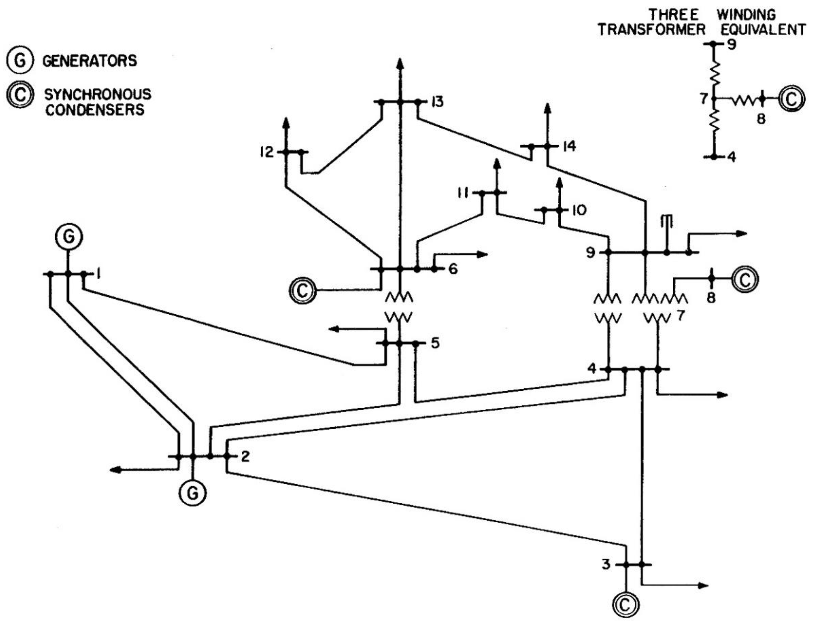
Figure 2. IEEE 14-node test system.

Figure 2. IEEE 14-node test system.

Figure 3. IEEE 30-node test system.

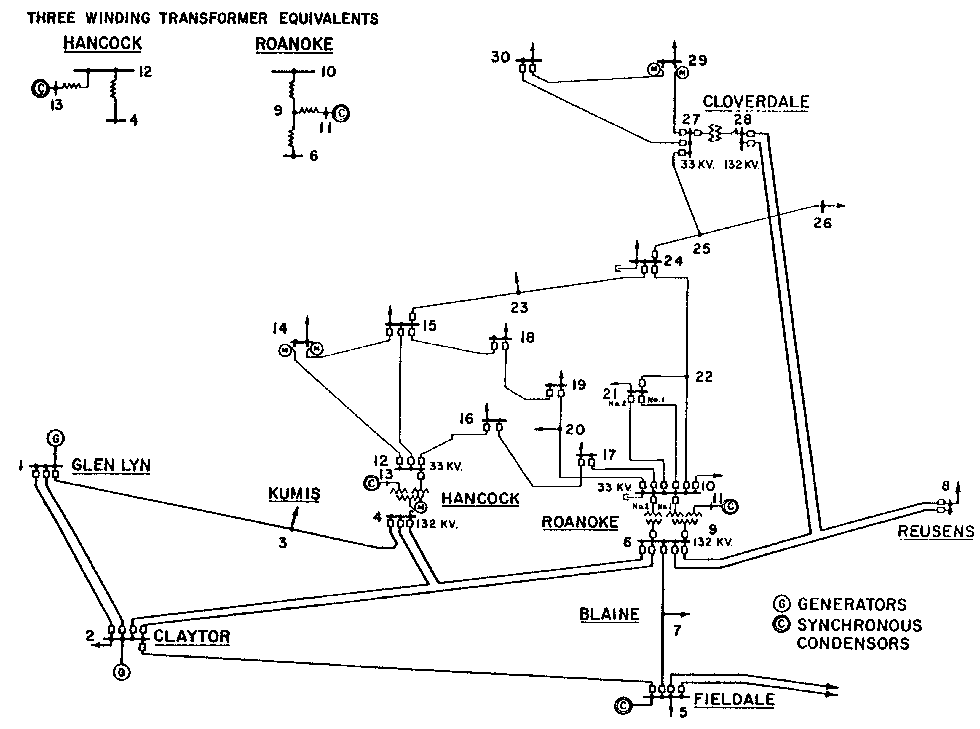
Figure 3. IEEE 30-node test system.

7.1. Case 0

The aim of this subsection is to present the results of the investigation for the entire area of the operating states of the IEEE 14-node TS. For this investigation, the name Case 0 is used. The investigation is carried out for the significance level α equal to 0.01.

In Table 1, there are relative numbers of CRs between the nodal-voltage magnitudes and the nodal reactive powers (in percentage), for particular ranges of absolute values of KRCCs. Each of these relative numbers is defined as the ratio of the number of CRs to the cardinality of the set S_V-Q (|S_V-Q|).

Table 1 shows that the largest absolute values of KRCC for CRs between the nodal-voltage magnitudes and the nodal reactive powers are in range [0.5, 0.6).

Table 1. The Numbers of CRs, whose absolute values of KRCC are in the Distinguished Ranges (in Percentage of all the Considered CRs).

Range of Absolute Values	Number of CRs, %
[0, 0.1)	75.00
[0.1, 0.2)	15.82
[0.2, 0.3)	5.61
[0.3, 0.4)	2.55
[0.4, 0.5)	0.51
[0.5, 0.6)	0.51
[0.6, 0.7)	0
[0.7, 0.8)	0
[0.8, 0.9)	0
[0.9, 1.0]	0

Table 1. The Numbers of CRs, whose absolute values of KRCC are in the Distinguished Ranges (in Percentage of all the Considered CRs).

Range of Absolute Values	Number of CRs, %
[0, 0.1)	75.00
[0.1, 0.2)	15.82
[0.2, 0.3)	5.61
[0.3, 0.4)	2.55
[0.4, 0.5)	0.51
[0.5, 0.6)	0.51
[0.6, 0.7)	0
[0.7, 0.8)	0
[0.8, 0.9)	0
[0.9, 1.0]	0

Based on Cohen’s standard,

Table 2. Rule of Thumb of Interpreting the Size of KRCC.

Strength of Association	KRCC
	Positive	Negative
Very small	<0.1	>−0.1
Small	[0.1, 0.3)	(−0.3, −0.1]
Medium	[0.3, 0.5)	(−0.5, −0.3]
Large	[0.5, 1.0]	[−1.0, −0.5]

presents the rule of thumb for interpreting the size of KRCC. It is easy to see that in the case of 75% of CRs, the strength of the association between the considered quantities can be evaluated as very small (negligible). Only in the case of 0.51% of all CRs (1 CR), the strength of the considered association is large, and in the case of 3.06% of all CRs (6 CRs), this strength is medium.

All KRCCs are subjected to the significance test. The numbers of SSCRs for the particular kinds of these CRs are in Table 3.

A part of the set S_V-Q, containing SSCRs, is referred to as S_S,V-Q. General characteristics of CRs in the set S_S,V-Q are given in Table 3. In that table, it is assumed that S_S-,V-Q, and S_S+,V-Q are sets of CRs with negative and positive KRCCs, respectively, and S_S,V-Q = S_S-,V-Q∪S_S+,V-Q. Analyzing Table 3, one can state that |S_S+,V-Q| = 26.9% |S_S,V-Q|.

Table 3. The Numbers of SSCRs for the Particular Kinds of these CRs (in Percentage of All CRs, i.e., in Percentage of |S_V-Q|).

Set of CRs	Cardinality of the Set
SS,V-Q	26.53
SS-,V-Q	19.39
SS+,V-Q	7.14

Table 3. The Numbers of SSCRs for the Particular Kinds of these CRs (in Percentage of All CRs, i.e., in Percentage of |S_V-Q|).

Set of CRs	Cardinality of the Set
SS,V-Q	26.53
SS-,V-Q	19.39
SS+,V-Q	7.14

Detailed characteristics of SSCRs between the nodal-voltage magnitudes and the nodal reactive powers are in

Table 4. Detailed Characteristics of SSCRs between Nodal Reactive Powers and Nodal-Voltage Magnitudes.

Min of KRCC	Max of KRCC	Average Value of Abs. Val. of KRCCs	Average Value of KRCCs	Average Value of Negative KRCCs	Average Value of Positive KRCCs
−0.249	0.517	0.198	−0.046	−0.169	0.285

. Table 4 shows such parameters of the set S_S,V-Q as (i) a minimum of KRCC, (ii) a maximum of KRCC, (iii) an average value of absolute values of KRCCs, (iv) an average value of KRCCs, (v) an average value of negative of KRCCs, and (vi) an average value of positive of KRCCs.

KRCCs for SSCRs are in

Table 5. Values of KRCCs Characterizing SSCRs between Nodal Reactive Powers and Nodal-Voltage Magnitudes (α = 0.01).

Qj	Vi	tk_Vi-Qj	Qj	Vi	tk_Vi-Qj	Qj	Vi	tk_Vi-Qj
Q1	V1	0.47		V5	−0.08		V6	0.19
	V5	0.13	Q6	V1	−0.20		V8	0.52
Q2	V1	−0.24		V2	−0.22		V9	−0.16
	V2	0.15		V3	−0.18		V10	−0.18
Q3	V1	−0.23		V4	−0.18		V11	−0.21
	V2	−0.25		V5	−0.15		V12	−0.19
	V3	0.25		V6	0.39		V13	−0.19
	V4	−0.14		V7	−0.17		V14	−0.20
	V5	−0.19		V8	−0.11	Q9	V1	−0.13
	V6	−0.13		V9	−0.14		V2	−0.13
	V7	−0.12		V11	0.18		V5	−0.10
	V9	−0.12		V12	0.35		V7	−0.16
	V10	−0.14		V13	0.32		V9	0.40
	V11	−0.15	Q8	V1	−0.19		V10	0.33
	V12	−0.14		V2	−0.24		V11	0.12
	V13	0.14		V3	−0.18		V14	0.22
	V14	−0.16		V4	−0.21
Q5	V4	−0.09		V5	−0.23

. The strongest CR among the considered ones is cr_V8-Q8. In Table 5, for each of the nodal powers, the strongest CR is indicated in bold font of the KRCC value. The cardinality of the set S_S,V-Q is equal to 52 (i.e., 26.53% of |S_V-Q|).

In Table 6, the ranking list R_AS,LS is shown; i.e., a ranking list of influence sets of the nodal reactive powers in PS, when the ranking criterion is the cardinality of a set. The set with the largest cardinality is at the top of the list. In the first and second positions of the list, there are the set A_S,8 and the set A_S,3. These sets have the same cardinality. The last column of Table 6 contains the index κ_S for the distinguished influence sets.

In each row of Table 6, one voltage magnitude is written in bold. This voltage magnitude is in the strongest CR with the nodal reactive power with which the considered influence set is associated.

Characteristics of CRs in the particular sets A_S,j j = 1, 2, 3, 5, 6, 8, 9 are in

Table 7. Characteristics of SSCRs Between Nodal-Voltage Magnitudes and Nodal Reactive Powers Related to Particular Sets A_S,j j = 1, 2, 3, 5, 6, 8, 9.

No.	Set	Number of CRs	Number of CRs with Negative KRCC	Number of CRs with Positive KRCC	Min of KRCC	Max of KRCC	Average Value of Abs. Val. of KRCCs	Average Value of KRCCs	Average Value of Negative KRCCs	Average Value of Positive KRCCs
1	AS,8	13	12	1	−0.24	0.52	0.22	−0.14	−0.20	0.52
2	AS,3	13	12	1	−0.25	0.25	0.21	−0.12	−0.16	0.25
3	AS,6	12	8	4	−0.22	0.39	0.22	−0.01	−0.17	0.31
4	AS,9	8	3	5	−0.13	0.40	0.20	0.11	−0.12	0.25
5	AS,1	2	0	2	0.13	0.47	0.30	0.30	0.00	0.30
6	AS,2	2	1	1	−0.24	0.15	0.20	−0.04	−0.24	0.15
7	AS,5	2	2	0	−0.09	−0.08	0.085	−0.085	−0.085	0.00

. For each of those sets, there are given (i) a cardinality, (ii) number of CRs with negative KRCC, (iii) number of CRs with positive KRCC, (iv) a minimum of KRCCs, (v) a maximum of KRCCs, (vi) an average value of absolute values of KRCCs, (vii) an average value of KRCCs, (viii) an average value of negative of KRCCs, and (ix) an average value of positive of KRCCs.

Table 6. The Ranking List of the Sets A_S,j j ∈ {1, 2, …, 14}, when the Cardinality of a Set is Adopted as a Criterion.

No.	Set	Content of Set	Index κS
1	AS,8	V1, V2, V3, V4, V5, V6, V8, V9, V10, V11, V12, V13, V14	2.91
2	AS,3	V1, V2, V3, V4, V5, V6, V7, V9, V10, V11, V12, V13, V14	2.15
3	AS,6	V1, V2, V3, V4, V5, V6, V7, V8, V9, V11, V12, V13	2.59
4	AS,9	V1, V2, V5, V7, V9, V10, V11, V14	1.57
5	AS,1	V1, V5	0.60
6	AS,2	V1, V2	0.40
7	AS,5	V4, V5	0.17

Table 6. The Ranking List of the Sets A_S,j j ∈ {1, 2, …, 14}, when the Cardinality of a Set is Adopted as a Criterion.

No.	Set	Content of Set	Index κS
1	AS,8	V1, V2, V3, V4, V5, V6, V8, V9, V10, V11, V12, V13, V14	2.91
2	AS,3	V1, V2, V3, V4, V5, V6, V7, V9, V10, V11, V12, V13, V14	2.15
3	AS,6	V1, V2, V3, V4, V5, V6, V7, V8, V9, V11, V12, V13	2.59
4	AS,9	V1, V2, V5, V7, V9, V10, V11, V14	1.57
5	AS,1	V1, V5	0.60
6	AS,2	V1, V2	0.40
7	AS,5	V4, V5	0.17

Table 8 shows the ranking list R_AD,LD; i.e., a ranking list of dominance sets of the nodal reactive powers in TS, when the ranking criterion is the cardinality of a set. There are only five such sets. The detailed parameters characterizing those sets (i.e., the sets A_D,j j = 1, 3, 6, 8, 9) are in Table 9.

The ranking list R_Q,κ; i.e., a ranking list of dominant nodal reactive powers, when a ranking criterion is the index κ, is given in Table 10. Its shortened version is as follows: Q₆, Q₈, Q₉, and Q₃.

Taking into account the presented considerations, it can be stated that the list of numbers of candidate nodes for the location of additional reactive power sources is 8, 6, 9, and 3. The given list contains the node numbers in the order resulting from the shortened ranking list of dominant nodal reactive powers.

Table 8. A Ranking List of Sets A_D,i i ∈ {1, 2, …, 14}, when the Index κ_D is Adopted as a Criterion.

No.	Set	Content of Set	Index κD
1	AD,6	V6, V7, V12, V13	1.23
2	AD,8	V4, V5, V8, V11	1.17
3	AD,9	V9, V10, V14	0.95
4	AD,3	V2, V3	0.50
5	AD,1	V1	0.47

Table 8. A Ranking List of Sets A_D,i i ∈ {1, 2, …, 14}, when the Index κ_D is Adopted as a Criterion.

No.	Set	Content of Set	Index κD
1	AD,6	V6, V7, V12, V13	1.23
2	AD,8	V4, V5, V8, V11	1.17
3	AD,9	V9, V10, V14	0.95
4	AD,3	V2, V3	0.50
5	AD,1	V1	0.47

Table 9. Characteristics of SSCRs Related to Particular Sets A_D,j j = 1, 3, 6, 8, 9.

No.	Set	Number of CRs	Number of CRs with Negative KRCC	Number of CRs with Positive KRCC	Min of KRCC	Max of KRCC	Average Value of Abs. Val. of KRCCs	Average Value of KRCCs	Average Value of Negative KRCCs	Average Value of Positive KRCCs
1	AD,6	4	1	3	−0.17	0.39	0.31	0.22	−0.17	0.35
2	AD,8	4	3	1	−0.23	0.52	0.29	−0.03	−0.22	0.52
3	AD,9	3	0	3	0.22	0.40	0.32	0.32	0.00	0.32
4	AD,3	2	1	1	−0.25	0.25	0.25	0.00	−0.25	0.25
5	AD,1	1	0	1	0.47	0.47	0.47	0.47	0.00	0.47

Table 9. Characteristics of SSCRs Related to Particular Sets A_D,j j = 1, 3, 6, 8, 9.

No.	Set	Number of CRs	Number of CRs with Negative KRCC	Number of CRs with Positive KRCC	Min of KRCC	Max of KRCC	Average Value of Abs. Val. of KRCCs	Average Value of KRCCs	Average Value of Negative KRCCs	Average Value of Positive KRCCs
1	AD,6	4	1	3	−0.17	0.39	0.31	0.22	−0.17	0.35
2	AD,8	4	3	1	−0.23	0.52	0.29	−0.03	−0.22	0.52
3	AD,9	3	0	3	0.22	0.40	0.32	0.32	0.00	0.32
4	AD,3	2	1	1	−0.25	0.25	0.25	0.00	−0.25	0.25
5	AD,1	1	0	1	0.47	0.47	0.47	0.47	0.00	0.47

Table 10. A Ranking List of the Dominant Nodal Reactive Powers when the Index κ is Adopted as Criterion.

No.	j	Qj	κj
1	8	Q8	3.40
2	6	Q6	3.19
3	9	Q9	1.49
4	3	Q3	1.07
5	1	Q1	0.29

Table 10. A Ranking List of the Dominant Nodal Reactive Powers when the Index κ is Adopted as Criterion.

No.	j	Qj	κj
1	8	Q8	3.40
2	6	Q6	3.19
3	9	Q9	1.49
4	3	Q3	1.07
5	1	Q1	0.29

7.2. Case 1, Case 2, and Case 3

The aim of this subsection is to present the investigation results for the selected areas of the considered operating states of the IEEE 14-node TS. The ranges of system active-power losses characterizing those areas are presented in Table 11. They are sub-ranges of the active-power loss range in Case 0.

The investigation is conducted for three cases. In Case 1, the system active-power losses are the smallest, and in Case 3, the losses are the largest ones. The definitions of all the considered cases are in Table 11. Then, the active power losses in Case 1 will be described as small, in Case 2—as medium, and in Case 3—as large.

Table 11. System Active-Power Losses Characterizing the Considered Study Cases.

Case	Range of System Active-Power Losses, pu	Evaluation of System Active-Power Losses
Case 1	[0.06, 0.13)	Small
Case 2	[0.13, 0.20)	Medium
Case 3	[0.20, 0.27]	Large

Table 11. System Active-Power Losses Characterizing the Considered Study Cases.

Case	Range of System Active-Power Losses, pu	Evaluation of System Active-Power Losses
Case 1	[0.06, 0.13)	Small
Case 2	[0.13, 0.20)	Medium
Case 3	[0.20, 0.27]	Large

In

Table 12. A Ranking List of the Dominant Nodal Reactive Powers when the Index κ is Adopted as Criterion for Case 1.

No.	j	Qj	κj
1	9	Q9	2.83
2	8	Q8	1.81
3	6	Q6	1.29
4	3	Q3	0.19
5	1	Q1	0.16

,

Table 13. A Ranking List of the Dominant Nodal Reactive Powers when the Index κ is Adopted as Criterion for Case 2.

No.	j	Qj	κj
1	8	Q8	2.90
2	9	Q9	1.81
3	5	Q5	1.67
4	6	Q6	0.50
5	3	Q3	0.21
6	1	Q1	0.16
7	2	Q2	0.06

and

Table 14. A Ranking List of the Dominant Nodal Reactive Powers when the Index κ is Adopted as Criterion for Case 3.

No.	j	Qj	κj
1	6	Q6	3.03
2	8	Q8	1.40
3	9	Q9	0.42
4	1	Q1	0.21
5	3	Q3	0.11

, ranking lists of the dominant nodal reactive powers for Case 1, Case 2, and Case 3 are presented.

Shortened ranking lists of the dominant nodal reactive powers for the considered study cases are as follows:

Case 1: Q₉, Q₈, Q₆, and Q₃;

Case 2: Q₈, Q₉, Q₅, Q₆, and Q₃;

Case 3: Q₆, Q₈, Q₉, and Q₃.

Based on the shortened lists of the dominant nodal reactive powers, it can be concluded that the ranking lists of candidate nodes for the location of additional reactive power sources, when the nodes are represented by their numbers, are as follows:

Case 1: 9, 8, 6, and 3;

Case 2: 8, 9, 5, 6, and 3;

Case 3: 6, 8, 9, and 3.

7.3. Case 4

The subsection presents the results of the search for candidate nodes for the location of additional reactive-power sources in the IEEE 30-node TS (Figure 3), which has larger dimensions than TS considered in Case 0, Case 1, Case 2, and Case 3.

Table 15. A Ranking List of the Dominant Nodal Reactive Powers when the Index κ is Adopted as Criterion for Case 4.

No.	j	Qj	κj
1	13	Q13	12.60
2	8	Q8	6.22
3	5	Q5	3.47
4	11	Q11	2.63
5	1	Q1	0.70
6	24	Q24	0.05

shows a ranking list of the dominant nodal reactive powers for the considered TS. The criterion for that ranking list is the index κ.

A shortened ranking list of the dominant nodal reactive powers for the considered study case is as follows:

Q₁₃, Q₈, Q₅, Q₁₁, and Q₂₄.

In this situation, the ranking list of candidate nodes for the location of additional reactive power sources is as follows:

13, 8, 5, 11 and 24.

8. Discussion

Section 8.1, Section 8.2, Section 8.3 and Section 8.4 contain a discussion of investigation results for the IEEE 14-node TS. The IEEE 30-node TS was included in the discussion presented in Section 8.5.

8.1. Statistically Significant Correlational Relationships

During analyses of CRs between the nodal-voltage magnitudes and the nodal reactive powers, it can be seen that the number of SSCRs is relatively small. The numbers of SSCRs as a percentage of the total number of possible CRs for individual study cases are given in

Table 16. The Numbers of SSCRs in Percentage of All CRs for Considered Study Cases for Different Values of the Significance Level α.

α	Case 0	Case 1	Case 2	Case 3
0.01	26.53	10.20	18.37	7.65
0.02	28.06	12.76	21.43	9.18
0.05	32.14	19.90	27.55	16.84
0.10	33.67	26.53	32.14	25.00

.

Table 16 shows that the numbers of SSCRs for Case 1, Case 2, and Case 3 are the closest to the number of SSCRs for Case 0, the greater the value of α. With α = 0.01, the numbers of SSCRs in Case 1, Case 2, and Case 3 account for 38.45%, 69.24%, and 28.84% of the number of SSCRs in Case 0, and when α = 0.1, already 78.79%, 95.46%, and 74.25% of the number of SSCRs in Case 0. From a statistical point of view, the best value for α is 0.01.

Considering Case 1, Case 2, and Case 3, it can be indicated that the number of SSCRs is the highest in Case 2, where, as was stated in Section 7.2, the active-power losses are medium. In Case 1, in which the system active-power losses are low; i.e., generally, the branch power flows are smaller than in Case 2; this means that the differences in magnitudes, as well as the differences in arguments of the voltages at the ends of the power-network branches, are smaller than in Case 2. As a result, the influence of individual nodal reactive powers on nodal-voltage magnitudes in the power network is smaller compared to Case 2. This fact can be used to explain the smaller number of SSCRs in Case 1 than in Case 2.

Based on the considerations in Section 4, it can be concluded that in the relationship between voltage magnitude V_i i ∈ I and power Q_j j ∈ I_Q (V_i = f(Q_j)), there may be many other quantities (distinguished in Section 4, in particular, nodal reactive powers), which modify this relationship. In Case 3, where the active power losses are larger than in Case 2, the influence of Q_j j ∈ I_Q on V_i i ∈ I is greater than in Case 2 (and also in Case 1), but at the same time, other quantities influencing the relationship V_i = f(Q_j) to a greater extent than in Case 1 or Case 2 modify this relationship, weakening the impact of Q_j j ∈ I_Q on V_i i ∈ I. As a result, the number of SSCRs is the smallest in Case 3 compared to Case 1 and Case 2.

It should be noted that the maximum absolute value of the KRCC for SSCRs is 0.462 for Case 1, 0.5 for Case 2, and 0.613 for Case 3, so it is the smallest one for Case 1 and the largest one for Case 2. For Case 0, the analyzed value is 0.517. It can therefore be concluded that the maximum absolute value of KRCC for SSCRs depends on the size of the system’s active-power losses. The greater these losses for a given study case, the greater the maximum absolute value of KRCC for SSCRs. Analyses show that also the average value of the absolute values of KRCCs for SSCRs is the highest for Case 3. This means that the strength of CRs is greatest in that study case.

8.2. Influence Sets and Dominance Sets

Comparing the numbers of the sets A_S,j and A_D,j j ∈ {1, 2, …, 14} for Case 0, Case 1, Case 2, and Case 3 (

Table 17. The Numbers of the Sets A_S,j and A_D,j j ∈ {1, 2, …, 14} for Considered Study Cases.

α	Influence Sets				Dominance Sets
	Case 0	Case 1	Case 2	Case 3	Case 0	Case 1	Case 2	Case 3
0.01	7	6	7	6	5	5	7	5
0.02	7	7	8	8	5	5	7	5
0.05	8	10	9	8	5	5	7	5
0.10	10	10	10	9	5	5	7	5

), we can note that these numbers can be different. Table 17 shows that as the significance level α increases, the number of the influence sets may increase. This is one of the consequences of the increasing number of CRs considered statistically significant. Another consequence is increasing the cardinality of the existing influence sets. In the case of the dominance sets, for each study case Case 0, Case 1, Case 2, and Case 3 taken separately, their number does not change when the constant α changes.

It should be noted that among sets A_S,j, as well as sets A_D,j j ∈ {1, 2, …, 14}, there are sets that contain only one element (

Table 18. The Numbers of One-Element Sets A_S,j and A_D,j j ∈ {1, 2, …, 14} for Considered Study Cases.

α	Influence Sets				Dominance Sets
	Case 0	Case 1	Case 2	Case 3	Case 0	Case 1	Case 2	Case 3
0.01	0	1	2	3	1	2	4	2
0.02	0	2	3	5	1	2	4	2
0.05	1	4	3	2	1	2	4	1
0.10	3	0	2	2	1	2	4	1

). Such sets are shown in Table 19, Table 20 and Table 21. Taking into account the influence sets, when α = 0.01, it can be said that each one-element set A_S,j j ∈ {1, 2, …, 14} is associated with the nodal reactive power, which is correlated with the magnitude of the voltage at the node at which this power is determined and this correlation is relatively strong. As α increases, we have an increasing number of one-element influence sets, each of which is defined as A_S,i = {V_j} i ≠ j. The strength of CRs, which are additionally taken into account for larger values of α, decreases with the increase in α. In the statistical sense, this tendency is related to the deterioration of the evaluation of the performed analyses along with the increase in the value of α.

The situation is different with regard to one-element dominance sets. For each value of α, in the case of each one-element set A_D,j j ∈ {1, 2, …, 14}, the set element is a value of the voltage magnitude V_j, being in the relationship cr_Vj-Qj, where Q_j is the nodal reactive power at node j and with which the considered set is associated; V_j is a magnitude of the voltage at node j. It should be noted that each of the aforementioned dominance sets contains the voltage magnitude that enters the CR with the highest statistical scores compared to the CRs between this voltage magnitude and the other nodal reactive powers.

Table 19. One-Element Influence Sets for Considered Study Cases when α = 0.01, 0.02.

α = 0.01				α = 0.02
Case 0	Case 1	Case 2	Case 3	Case 0	Case 1	Case 2	Case 3
	AS,1 = {V1}	AS,1 = {V1},	AS,1 = {V1},		AS,1 = {V1},	AS,1 = {V1},	AS,1 = {V1},
		AS,2= {V2}	AS,2= {V2},		AS,11= {V12}	AS,2= {V2},	AS,2 = {V2},
			AS,3= {V3}			AS,7= {V1}	AS,3 = {V3},
							AS,7 = {V1},
							AS,14 = {V7}

Table 19. One-Element Influence Sets for Considered Study Cases when α = 0.01, 0.02.

α = 0.01				α = 0.02
Case 0	Case 1	Case 2	Case 3	Case 0	Case 1	Case 2	Case 3
	AS,1 = {V1}	AS,1 = {V1},	AS,1 = {V1},		AS,1 = {V1},	AS,1 = {V1},	AS,1 = {V1},
		AS,2= {V2}	AS,2= {V2},		AS,11= {V12}	AS,2= {V2},	AS,2 = {V2},
			AS,3= {V3}			AS,7= {V1}	AS,3 = {V3},
							AS,7 = {V1},
							AS,14 = {V7}

Table 20. One-Element Influence Sets for Considered Study Cases when α = 0.05, 0.1.

α = 0.05				α = 0.1
Case 0	Case 1	Case 2	Case 3	Case 0	Case 1	Case 2	Case 3
AS,14 = {V14}	AS,1 = {V1},	AS,1 = {V1},	AS,1 = {V1},	AS,10 = {V6},		AS,7 = {V1},	AS,7 = {V1},
	AS,7 = {V8},	AS,7 = {V1},	AS,7 = {V1}	AS,11 = {V3},		AS,12 = {V1}	AS,10 = {V3}
	AS,13 = {V13}	AS,12 = {V1}		AS,14 = {V14}

Table 20. One-Element Influence Sets for Considered Study Cases when α = 0.05, 0.1.

α = 0.05				α = 0.1
Case 0	Case 1	Case 2	Case 3	Case 0	Case 1	Case 2	Case 3
AS,14 = {V14}	AS,1 = {V1},	AS,1 = {V1},	AS,1 = {V1},	AS,10 = {V6},		AS,7 = {V1},	AS,7 = {V1},
	AS,7 = {V8},	AS,7 = {V1},	AS,7 = {V1}	AS,11 = {V3},		AS,12 = {V1}	AS,10 = {V3}
	AS,13 = {V13}	AS,12 = {V1}		AS,14 = {V14}

Table 21. One-Element Dominance Sets for Considered Study Cases.

α = 0.01, 0.02				α = 0.05, 0.1
Case 0	Case 1	Case 2	Case 3	Case 0	Case 1	Case 2	Case 3
AD,1 = {V1}	AD,1 = {V1},	AD,1 = {V1},	AD,1 = {V1},	AD,1 = {V1}	AD,1 = {V1},	AD,1 = {V1},	AD,1 = {V1}
		AD,2 = {V2},				AD,2 = {V2},
	AD,3 = {V3}	AD,3 = {V3},	AD,3 = {V3}		AD,3 = {V3}	AD,3 = {V3},
		AD,6 = {V6}				AD,6 = {V6}

Table 21. One-Element Dominance Sets for Considered Study Cases.

α = 0.01, 0.02				α = 0.05, 0.1
Case 0	Case 1	Case 2	Case 3	Case 0	Case 1	Case 2	Case 3
AD,1 = {V1}	AD,1 = {V1},	AD,1 = {V1},	AD,1 = {V1},	AD,1 = {V1}	AD,1 = {V1},	AD,1 = {V1},	AD,1 = {V1}
		AD,2 = {V2},				AD,2 = {V2},
	AD,3 = {V3}	AD,3 = {V3},	AD,3 = {V3}		AD,3 = {V3}	AD,3 = {V3},
		AD,6 = {V6}				AD,6 = {V6}

In the case of influence sets, in Case 0 for α = 0.01, 0.02, and Case 1 for α = 0.1, there are no one-element sets. In each of the study cases: Case 1, Case 2, and Case 3 for α = 0.01, 0.02, 0.05 there is a set containing V₁, which is associated with the power Q₁. In Case 2, as well as in Case 3, for α = 0.01, 0.02 there is a one-element set containing V₂, which is associated with the power Q₂. It should be noted that node 1 and node 2 are generation nodes.

In the case of dominance sets, in each of the considered study cases (i.e., in Case 0, Case 1, Case 2, and Case 3), regardless of the value of α, also there is the one-element set containing V₁, which is associated with the power Q₁ (Table 21). The one-element set A_S,2 = {V₂,} is in Case 2, regardless of the value of α. One should pay attention to the one-element set containing V₃, which is associated with the power Q₃. Such a set is in Case 1, Case 2, and Case 3 for α = 0.01, 0.02, and in Case 1 and Case 2 for α = 0.05, 0.1.

The analysis of the influence sets in the study cases under consideration shows that regardless of the value of α in each study case, the nodal reactive powers, with which these influence sets are associated, are Q₁, Q₂, Q₃, Q₆, Q₈, and Q₉. Additionally, in Case 0 and Case 2, there are influence sets associated with the power Q₅. It turns out that the power system nodes with the mentioned powers are in the first part of the ranking list based on the index defined as follows:

$$Z_i={\sigma }_{Vi}/{{\displaystyle \sum }}_{i=1}^n{\sigma }_{Vi}+{\sigma }_{Qi}/{{\displaystyle \sum }}_{i=1}^n{\sigma }_{Qi}+c{\sigma }_{\delta i}/{{\displaystyle \sum }}_{i=1}^n{\sigma }_{\delta i}, i\in I_Q,$$

(20)

where

$${\sigma }_X=\sqrt{m^{-1}{{\displaystyle \sum }}_{j=1}^m{\left(d_{Xj}-m^{-1}{{\displaystyle \sum }}_{j=1}^m{d}_{Xj}\right)}^2}, X\in \{V_i, Q_i, {\delta }_i\},$$

(21)

c =0.39 (coefficient c is determined experimentally); j—a number of a data item of quantity X; m—the number of all data of quantity X; and d_Xj—j-th data item of quantity X.

${\sigma }_X$ is a measure of the variability of the quantity X. ${\sigma }_{Vi}/{{\displaystyle \sum }}_{i=1}^n{\sigma }_{Vi}$, ${\sigma }_{Qi}/{{\displaystyle \sum }}_{i=1}^n{\sigma }_{Qi}$, and ${\sigma }_{\delta i}/{{\displaystyle \sum }}_{i=1}^n{\sigma }_{\delta i}$ are standardized measures of the variability of V_i, Q_i, and δ_i, respectively.

For the considered study cases, the ranking lists of the test-system nodes, when the index Z is taken into account, are in Table 22. In that table, some TS nodes are distinguished by:

(i)

The shading, when at the nodes, there are the nodal reactive powers with which the existing influence sets are associated;

(ii)

The darker shading, when at the nodes, there are nodal reactive powers with which the existing dominance sets are associated.

Table 22. The ranking list of the TS nodes, when a ranking criterion is the index Z, for considered study cases.

No.	Case 0		Case 1		Case 2		Case 3
	i	Zi	i	Zi	i	Zi	i	Zi
1	1	6.99	6	9.62	6	7.63	2	6.19
2	2	5.05	9	4.58	2	3.76	1	5.34
3	6	3.05	2	3.25	1	3.48	9	3.18
4	9	2.97	8	1.81	9	2.91	6	3.11
5	8	2.37	3	1.64	8	2.53	8	2.58
6	3	1.92	1	1.59	3	1.94	3	1.66
7	5	1.467	12	1.401	5	1.42	12	1.52
8	12	1.466	13	1.396	12	1.41	13	1.48
9	13	1.45	14	1.374	13	1.39	5	1.47
10	4	1.43	10	1.371	4	1.383	4	1.38
11	14	1.38	11	1.31	10	1.378	14	1.37
12	10	1.37	5	1.28	14	1.35	10	1.33
13	11	1.35	4	1.26	11	1.3	11	1.32
14	7	1.20	7	1.19	7	1.21	7	1.14

Table 22. The ranking list of the TS nodes, when a ranking criterion is the index Z, for considered study cases.

No.	Case 0		Case 1		Case 2		Case 3
	i	Zi	i	Zi	i	Zi	i	Zi
1	1	6.99	6	9.62	6	7.63	2	6.19
2	2	5.05	9	4.58	2	3.76	1	5.34
3	6	3.05	2	3.25	1	3.48	9	3.18
4	9	2.97	8	1.81	9	2.91	6	3.11
5	8	2.37	3	1.64	8	2.53	8	2.58
6	3	1.92	1	1.59	3	1.94	3	1.66
7	5	1.467	12	1.401	5	1.42	12	1.52
8	12	1.466	13	1.396	12	1.41	13	1.48
9	13	1.45	14	1.374	13	1.39	5	1.47
10	4	1.43	10	1.371	4	1.383	4	1.38
11	14	1.38	11	1.31	10	1.378	14	1.37
12	10	1.37	5	1.28	14	1.35	10	1.33
13	11	1.35	4	1.26	11	1.3	11	1.32
14	7	1.20	7	1.19	7	1.21	7	1.14

Indeed, the index Z_i refers to CR cr_Vi-Qi i ∈ {1, 2, …,14}. However, any such CR, so long as it is SSCR, relates to a voltage magnitude that is in some influence set. In the considered case, the voltage magnitude is V_i, and the mentioned influence set is A_S,i, with which the reactive power Q_i is associated; i.e., this nodal reactive power is at the same node as the voltage magnitude V_i. Therefore, the aforementioned ranking list can be associated with the existing influence sets. It should be emphasized that there is no influence set without the magnitude of the voltage at the node at which there is the nodal reactive power associated with the mentioned set. In most cases, KRCC of cr_Vi-Qi is maximal or close to the maximal value of KRCCs of CRs cr_Vi-Qj i = i₁, i₂, …, i_cj, where I_S,j = {i₁, i₂, …, i_cj}; I_S,j—a set of indices of the voltages whose magnitudes are in the influence set A_S,j; c_j = |A_S,j|.

It should be noted that in addition to the previously mentioned influence sets associated with Q₁, Q₂, Q₃, Q₆, Q₈, and Q₉ and eventually with Q₅, for α > 0.01, influence sets associated with other nodal reactive powers can occur. However, the statistical evaluation of those sets is inferior compared to the sets associated with Q₁, Q₂, Q₃, Q₆, Q₈, Q₉, and Q₅.

The same nodal-voltage magnitude can be in more than one influence set A_S,j j ∈ {1, 2, …, 14}. This is a consequence of the fact that more than one nodal reactive power can have a significant influence on a given nodal-voltage magnitude. This voltage magnitude is in the set A_D,j j ∈ {1, 2, …, 14}, which is associated with the nodal reactive power having the greatest influence on the considered voltage magnitude.

If significance level α changes from 0.01 to 0.1, we can observe that:

• The number of SSCRs changes (Table 16).
• In the case of some influence sets, their cardinalities do not change—such sets are (i) A_S,2 for Case 0, (ii) A_S,3 for Case 0 and Case 1, and (iii) A_S,9 for Case 1.
• Taking into account the ranking list of influence sets, when a ranking criterion is the cardinality of a set (R_AS,c where c stands for the cardinality of the set A_S), we can state that:
  • In Case 0, influence sets that are ranked for α = 0.01 do not change rank for α > 0.01; there is no such regularity in other study cases, i.e., in Case 1, Case 2, or Case 3;
  • In Case 0, Case 1, and Case 3, the relation between the numbers of the positions in the ranking list R_AS,c taken by the sets associated with the dominant nodal reactive powers does not change with changes in α; this statement also applies to Case 2, provided that the dominant nodal reactive powers, with which single-element dominance sets are associated, are omitted.
• Taking into account the ranking list of influence sets, when a ranking criterion is the index κ_I (R_AS,κ_I), we can state that:
  • In Case 0, the influence sets distinguished for α = 0.01 being in the first five positions of the ranking list R_AS,κ_I, are in the same position in the ranking list R_AS,κ_I for each α satisfying the condition α > 0.01; the same can be seen in Case 2 for the first three positions and in Case 3 for the first two positions in the ranking list R_AS,κ_I.
  • In Case 0, the relation between the numbers of the positions in the ranking list taken by the sets associated with the dominant nodal reactive powers does not change with changes in α; the statement does not apply in Case 1, Case 2, and Case 3.
• Generally, for the same case and the same significance level α, both previously considered ranking lists of the influence sets (i.e., R_AS,c and R_AS,κ_I) are different. When two influence sets are considered, the higher position of one of them on the ranking list R_AS,c does not mean that it will occupy a higher position in relation to the second set on the ranking list R_AS,κ_I.
• Taking into account the ranking list of dominance sets, when a ranking criterion is the cardinality of a set (R_AD,c), as well as when a ranking criterion is the index κ_D (R_AD,κ_D), we can state that in each of the cases: Case 0, Case 1, and Case 2, both the ranking lists are independent from α. For the ranking list R_AD,κ_D, in Case 3, the three first positions of the ranking list are also independent from α.
• Comparing both aforementioned ranking lists of the dominance sets (i.e., R_AD,c and R_AD,κ_D), we can observe the identity of these lists in each of the cases: Case 0, Case 1, and Case 2. In Case 3, the differences between those lists are in the first two positions.

8.3. Evaluation of Dominant Nodal Reactive Powers with the Use of the Index κ

This subsection considers the dominant nodal reactive powers (for the IEEE 14-node TS); i.e., these powers with which dominance sets are associated, in the context of their evaluation with the use of the index κ. The influence sets related to the mentioned powers, which are taken into account when determining the ranking of dominant nodal reactive powers, are included in the analysis.

CRs between nodal-voltage magnitudes and dominant nodal reactive powers, which are the strongest from the point of view of individual powers, are given in Table 23. Taking into account the rules given in Table 2, it can be concluded that in Table 23, there is only one relationship in each of the cases: Case 0, Case 2, and Case 3, in which the strength of the association between the considered quantities can be evaluated as large. In the case of the remaining relationships, the strength of association between the quantities taken into account is medium or low. In Table 23, the latter relationships are the fewest. These are CRs: in Case 0—cr_V3-Q3; in Case 2—cr_V2-Q2, cr _V3-Q3, and cr_V11-Q5.

In each of the study cases: Case 0, Case 1, Case 2, and Case 3, the strongest CR is cr_V8-Q8; i.e., the CR between the magnitude of the nodal-voltage V₈ and the nodal reactive power Q₈. In effect, the voltage magnitude V₈ is not only in the set A_S,8, but also in the set A_D,8.

The cardinality of the influence sets associated with the dominant nodal reactive powers in Case 0, Case 1, Case 2, and Case 3 are in Table 24. Table 25 shows indices κ_S,j, where j is an element of the set of indices of the nodes at which there are the dominant nodal reactive powers.

Table 23. Nodal Reactive Powers and Nodal-Voltage Magnitudes between which There Are the Strongest CRs (from the Point of View of the Considered Power) and KRCCs Characterizing These CRs for Case 0, Case 1, Case 2, and Case 3.

Case 0			Case 1			Case 2			Case 3
Qj	Vi	tk_Vi-Qj	Qj	Vi	tk_Vi-Qj	Qj	Vi	tk_Vi-Qj	Qj	Vi	tk_Vi-Qj
Q8	V8	0.517	Q8	V8	0.462	Q8	V8	0.500	Q8	V8	0.613
Q1	V1	0.474	Q9	V9	0.457	Q9	V9	0.444	Q1	V1	0.455
Q9	V9	0.397	Q1	V1	0.395	Q1	V1	0.396	Q6	V6	0.451
Q6	V6	0.385	Q3	V3	0.336	Q6	V6	0.302	Q9	V9	0.367
Q3	V3	0.249	Q6	V6	0.330	Q3	V3	0.278	Q3	V3	0.338
						Q5	V11	0.267
						Q2	V2	0.243

Table 23. Nodal Reactive Powers and Nodal-Voltage Magnitudes between which There Are the Strongest CRs (from the Point of View of the Considered Power) and KRCCs Characterizing These CRs for Case 0, Case 1, Case 2, and Case 3.

Case 0			Case 1			Case 2			Case 3
Qj	Vi	tk_Vi-Qj	Qj	Vi	tk_Vi-Qj	Qj	Vi	tk_Vi-Qj	Qj	Vi	tk_Vi-Qj
Q8	V8	0.517	Q8	V8	0.462	Q8	V8	0.500	Q8	V8	0.613
Q1	V1	0.474	Q9	V9	0.457	Q9	V9	0.444	Q1	V1	0.455
Q9	V9	0.397	Q1	V1	0.395	Q1	V1	0.396	Q6	V6	0.451
Q6	V6	0.385	Q3	V3	0.336	Q6	V6	0.302	Q9	V9	0.367
Q3	V3	0.249	Q6	V6	0.330	Q3	V3	0.278	Q3	V3	0.338
						Q5	V11	0.267
						Q2	V2	0.243

Table 24. The Cardinality of the Influence Sets Associated with the Dominant Nodal Reactive Powers in Case 0, Case 1, Case 2, and Case 3.

	α = 0.01				α = 0.02				α = 0.05				α = 0.1
Set	Case 0	Case 1	Case 2	Case 3	Case 0	Case 1	Case 2	Case 3	Case 0	Case 1	Case 2	Case 3	Case 0	Case 1	Case 2	Case 3
AS.1	2	1	1	1	2	1	1	1	3	1	1	1	3	2	3	2
AS.2			1				1				3				3
AS.3	13	2	3	1	13	2	4	1	13	2	9	8	13	2	10	10
AS.5			10				10				11				12
AS.6	12	5	7	6	12	6	9	6	14	9	11	8	13	10	12	11
AS.8	13	5	10	4	13	8	11	5	14	12	11	6	14	13	12	10
AS.9	8	5	4	2	9	5	5	2	12	5	6	4	12	5	6	8

Table 24. The Cardinality of the Influence Sets Associated with the Dominant Nodal Reactive Powers in Case 0, Case 1, Case 2, and Case 3.

	α = 0.01				α = 0.02				α = 0.05				α = 0.1
Set	Case 0	Case 1	Case 2	Case 3	Case 0	Case 1	Case 2	Case 3	Case 0	Case 1	Case 2	Case 3	Case 0	Case 1	Case 2	Case 3
AS.1	2	1	1	1	2	1	1	1	3	1	1	1	3	2	3	2
AS.2			1				1				3				3
AS.3	13	2	3	1	13	2	4	1	13	2	9	8	13	2	10	10
AS.5			10				10				11				12
AS.6	12	5	7	6	12	6	9	6	14	9	11	8	13	10	12	11
AS.8	13	5	10	4	13	8	11	5	14	12	11	6	14	13	12	10
AS.9	8	5	4	2	9	5	5	2	12	5	6	4	12	5	6	8

Table 24 shows that in each of the study cases: Case 0, Case 1, and Case 2, among the considered influence sets, there is no set of greater cardinality than that of the set A_S,8. In Case 3, only the cardinality of A_S,6 is greater than |A_S,8|. The power Q₈ therefore has an influence on the relatively large area of TS. The power Q₈ has also a relatively large influence on the voltage magnitudes in the mentioned area. This observation results from the analysis of Table 25. It takes place that (i) κ_S.8 > κ_S.i i = 1, 3, 6, 9 for Case 0; (ii) κ_S.8 > κ_S.i i = 1, 3, 6 for Case 1; (iii) κ_S.8 > κ_S.i i = 1, 2, 3, 5, 6, 9 for Case 2; and (iv) κ_S.8 > κ_S.i i = 1, 3, 9 for Case 3. Such a large influence of the power Q₈ on the voltages in TS can be explained by the location of node 8. Note that node 8 is connected to the third winding of the transformer, which is between the higher-voltage part of TS and the lower-voltage part of TS.

As in cr_V8-Q8, in cr_V6-Q6 and cr_V9-Q9, there are the nodal reactive powers (Q₆ and Q₉) at the nodes to which transformers are connected. Those transformers are between the higher-voltage part of TS and the lower-voltage part of this system. The influence sets associated with the powers Q₆ and Q₉ have high cardinalities (Table 24) and are also characterized by high values of the indices κ_S.6 and κ_S.9, respectively (Table 25). It can therefore be concluded that the mentioned powers have a significant influence on the nodal-voltage magnitudes in TS. It should be noted that in Case 0, Case 1, and Case 3, for α ≠ 0.05, the powers Q₆, Q₈, and Q₉ are in the first three positions of the ranking list R_Dr,κ; i.e., the ranking list of dominant nodal reactive powers when a ranking criterion is the index κ (Equation (18)) (Table 26). In Case 2, the power Q₅ is among the first three dominant powers in the ranking list R_Dr,κ, which in addition to that power are the powers Q₈ and Q₉. The power Q₅ is in the third position of that ranking list. The power Q₆ is in the fourth position of the mentioned ranking list. In Case 3 for α = 0.05, the power Q₃ is in the third position of the considered ranking list and the power Q₉ is in the fourth position of this list.

Table 25. Indices κ_S,j Characterizing Influence Sets Associated with Dominant Nodal Reactive Powers in Case 0. Case 1. Case 2 and Case 3.

	α = 0.01				α = 0.02				α = 0.05				α = 0.1
Index	Case 0	Case 1	Case 2	Case 3	Case 0	Case 1	Case 2	Case 3	Case 0	Case 1	Case 2	Case 3	Case 0	Case 1	Case 2	Case 3
κS.1	0.60	0.40	0.40	0.45	0.60	0.40	0.40	0.45	0.68	0.40	0.40	0.45	0.68	0.54	0.66	0.60
κS.2			0.24				0.24				0.55				0.55
κS.3	2.15	0.57	0.74	0.34	2.15	0.57	0.94	0.34	2.15	0.57	1.76	1.47	2.15	0.57	1.90	1.74
κS.5			2.35				2.35				2.51				2.66
κS.6	2.59	1.42	1.67	1.98	2.59	1.61	2.05	1.98	2.66	2.10	2.37	2.31	2.66	2.24	2.51	2.72
κS.8	2.90	1.46	2.69	1.30	2.90	2.01	2.88	1.48	2.97	2.65	2.88	1.66	2.97	2.77	3.02	2.21
κS.9	1.57	1.68	1.35	0.65	1.65	1.68	1.53	0.65	1.86	1.68	1.69	0.98	1.86	1.68	1.69	1.51

Table 25. Indices κ_S,j Characterizing Influence Sets Associated with Dominant Nodal Reactive Powers in Case 0. Case 1. Case 2 and Case 3.

	α = 0.01				α = 0.02				α = 0.05				α = 0.1
Index	Case 0	Case 1	Case 2	Case 3	Case 0	Case 1	Case 2	Case 3	Case 0	Case 1	Case 2	Case 3	Case 0	Case 1	Case 2	Case 3
κS.1	0.60	0.40	0.40	0.45	0.60	0.40	0.40	0.45	0.68	0.40	0.40	0.45	0.68	0.54	0.66	0.60
κS.2			0.24				0.24				0.55				0.55
κS.3	2.15	0.57	0.74	0.34	2.15	0.57	0.94	0.34	2.15	0.57	1.76	1.47	2.15	0.57	1.90	1.74
κS.5			2.35				2.35				2.51				2.66
κS.6	2.59	1.42	1.67	1.98	2.59	1.61	2.05	1.98	2.66	2.10	2.37	2.31	2.66	2.24	2.51	2.72
κS.8	2.90	1.46	2.69	1.30	2.90	2.01	2.88	1.48	2.97	2.65	2.88	1.66	2.97	2.77	3.02	2.21
κS.9	1.57	1.68	1.35	0.65	1.65	1.68	1.53	0.65	1.86	1.68	1.69	0.98	1.86	1.68	1.69	1.51

Table 26. Ranking Lists of Dominate Nodal Reactive Powers when a Ranking Criterion is the Index κ for Different Study Cases and Different Values of Level α.

α = 0.01				α = 0.02				α = 0.05				α = 0.1
Case 0	Case 1	Case 2	Case 3	Case 0	Case 1	Case 2	Case 3	Case 0	Case 1	Case 2	Case 3	Case 0	Case 1	Case 2	Case 3
Q8	Q9	Q8	Q6	Q8	Q9	Q8	Q6	Q8	Q8	Q8	Q6	Q8	Q8	Q8	Q6
Q6	Q8	Q9	Q8	Q6	Q8	Q9	Q8	Q6	Q9	Q9	Q8	Q6	Q9	Q9	Q8
Q9	Q6	Q5	Q9	Q9	Q6	Q5	Q9	Q9	Q6	Q5	Q3	Q9	Q6	Q5	Q9
Q3	Q3	Q6	Q1	Q3	Q3	Q6	Q1	Q3	Q3	Q6	Q9	Q3	Q1	Q6	Q3
Q1	Q1	Q3	Q3	Q1	Q1	Q3	Q3	Q1	Q1	Q3	Q1	Q1	Q3	Q3	Q1
		Q1				Q1				Q1				Q1
		Q2				Q2				Q2				Q2

Table 26. Ranking Lists of Dominate Nodal Reactive Powers when a Ranking Criterion is the Index κ for Different Study Cases and Different Values of Level α.

α = 0.01				α = 0.02				α = 0.05				α = 0.1
Case 0	Case 1	Case 2	Case 3	Case 0	Case 1	Case 2	Case 3	Case 0	Case 1	Case 2	Case 3	Case 0	Case 1	Case 2	Case 3
Q8	Q9	Q8	Q6	Q8	Q9	Q8	Q6	Q8	Q8	Q8	Q6	Q8	Q8	Q8	Q6
Q6	Q8	Q9	Q8	Q6	Q8	Q9	Q8	Q6	Q9	Q9	Q8	Q6	Q9	Q9	Q8
Q9	Q6	Q5	Q9	Q9	Q6	Q5	Q9	Q9	Q6	Q5	Q3	Q9	Q6	Q5	Q9
Q3	Q3	Q6	Q1	Q3	Q3	Q6	Q1	Q3	Q3	Q6	Q9	Q3	Q1	Q6	Q3
Q1	Q1	Q3	Q3	Q1	Q1	Q3	Q3	Q1	Q1	Q3	Q1	Q1	Q3	Q3	Q1
		Q1				Q1				Q1				Q1
		Q2				Q2				Q2				Q2

For middle values of the active power losses in TS (i.e., for Case 2), the cardinality of the set A_S,5 is equal to the maximum value of cardinalities of the sets A_S,i i = 1, 2, 3, 6, 8, 9, or it is only one lower than this value depending on the value α. The value of the index κ_S,5 is lower only than the value of the index κ_S,8. Due to the index κ_D,5, in the set D_R, the power Q₅ is in the third position in the ranking list R_Dr,κ_D. The situation is completely different in the other cases of the active power losses in TS, i.e., in Case 0, Case 1, and Case 3. In each of those cases, there is (i) a different relation between the cardinality of the set A_S,5 and the cardinalities of other influence sets, (ii) a different relation between the index κ_S,5 and the indices κ_S,j j ∈ I_AS j ≠ 5, characterizing other influence sets; and (iii) there is no set A_D,5 and, therefore, power Q₅ is not on the ranking list R_Dr,c nor on the ranking list R_Dr,κ_D. It should be added to the presented considerations that the power Q₅ is at the node connected to the higher-voltage winding of the transformer, being between the higher-voltage part of TS and the lower-voltage part of this system. As the analyses show, this fact plays an important role when the system active-power losses are of a middle value.

In the set D_R of each of the cases: Case 0, Case 1, Case 2, and Case 3, there is power Q₃. Analyzing Table 24, one can note that (i) |A_S.3| = |A_S.8|; i.e., |A_S.3| is equal to the maximum value of cardinalities of the considered influence sets in Case 0 when α = 0.01, 0.02 and Case 3 when α = 0.05, (ii) |A_S.3| is one less than the maximum value of cardinalities of the considered influence sets in Case 0 when α = 0.05, 0.1 and Case 3 when α = 0.1, and (iii) |A_S.3| is significantly smaller than the maximum value of cardinalities of the considered influence sets in other cases and when values of the level α are other than mentioned above. In the ranking list R_Dr,κ_D, the power Q₃ is in:

• Fourth position in Case 0 for α = 0.01, 0.02, 0.05, 0.1 and Case 3 for α = 0.05, 0.1;
• Fifth position in Case 1 for α = 0.01, 0.02, 0.05, 0.1 and Case 3 for α = 0.01, 0.02;
• Sixth position in Case 2 for α = 0.01, 0.02, 0.05, 0.1.

In effect, in ranking list R_Dr,κ, power Q₃ is in:

• Third position in Case 3 for α = 0.05;
• Fourth position in Case 0, Case 1 for α = 0.01, 0.02, 0.05, Case 0 for α = 0.1, and Case 3 for α = 0.1;
• Fifth position in Case 1 for α = 0.1, Case 2 for α = 0.01, 0.02, 0.05, 0.1, and Case 3 for α = 0.01, 0.02.

Thus, in general, the influence of the power Q₃ on the magnitudes of the voltages in TS is smaller than the power Q₆, Q₈, and Q₉. This is understandable due to the location of nodes 6, 8, and 9 in TS.

We can see in Table 23 that among the strongest CRs, there are also cr_V1-Q1 (Case 0, Case 1, Case 2, and Case 3), and cr_V2-Q2 (Case 2). In these CRs, there are nodal reactive powers at the generator nodes. These powers have a relatively strong influence on the magnitudes of the voltages at the nodes where they are, and possibly at neighboring nodes. We can see that Q₁ in Case 0, and Q₂ in Case 0 and Case 1 significantly influence the magnitudes of the voltages at one of the nodes adjacent to node 1 or 2, respectively. The low cardinality of A_S,1 and a relatively low position of the power Q₁ in the ranking list R_Dr,κ_D; i.e.,

• The last position in Case 0, for α = 0.01, 0.02, 0.05, 0.1, and Case 3 for α = 0.05, 0.1;
• The fourth position in Case 2, for α = 0.01, 0.02, 0.05, 0.1;
• The one before the last position in other cases than those mentioned above means that the power Q₁ is at the end of the ranking list R_Dr,κ; i.e.,
• In the last position in Case 0, Case 1 for α = 0.01, 0.02, 0.05, Case 0 for α = 0.1, and Case 3 for α = 0.05, 0.1;
• In the one before the last position in other cases than those mentioned above.

Only in Case 3 is the power Q₂ among the dominant nodal reactive powers (Table 23). In Case 3, the power Q₂ is in the last position of the ranking list of the dominant nodal reactive powers (Table 26).

It should be noted that for each dominant reactive power, there is the CR between that power and a magnitude of the voltage at the node where this power is present. Except for the power Q₅, the KRCC value for the earlier-mentioned CR is the largest, when we take into account the set of CRs of the power under consideration.

The list of the dominant reactive powers is different for the distinguished cases: Case 0, Case 1, Case 2, and Case 3. In each of the mentioned cases, this list includes the powers: Q₁, Q₃, Q₆, Q₈, and Q₉. It should be noted that:

• The listed powers are ordered differently in each of the cases;
• In Case 2, there are also Q₂ and Q₅ in the list under consideration.

For each value of α and each of the study cases: Case 0, Case 1, and Case 2, the ranking list R_Dr,κ is different from the ranking list R_Dr,κ_D. In Case 3, independently from α, the ranking list R_Dr,κ is the same as the ranking list R_Dr,κ_D. The presented facts are a consequence of taking into account not only the evaluation of the dominance sets, but also the evaluation of the influence sets when establishing the ranking list R_Dr,κ. It should be underlined that taking into account the evaluation of the influence sets may or may not change ranking list R_Dr,κ in relation to ranking list R_Dr,κ_D.

In Case 0, as well as Case 2, the ranking list R_Dr,κ does not depend on significance level α. In Case 3, only the two first positions of the ranking list R_Dr,κ do not depend on level α. Note that also in each of the study cases: Case 1 and Case 3, the ranking list R_Dr,κ will not change when α = 0.02 is taken instead of α = 0.01. It is obvious, from a statistical point of view, that the results of the analyses are rated higher for α = 0.01 or α = 0.02 than for α > 0.02.

8.4. Candidate Node for Installing Additional Sources of Reactive Power

Ranking lists of candidate nodes for the location of additional reactive-power sources (R_C,κ-s) are determined on the basis of the ranking lists of the dominant nodal reactive powers (R_Dr,κ-s), which are shown in Table 26 for the different study cases and the different values of the level α, excluding generation nodes (i.e., nodes 1 and possibly 2) from these lists. The ranking lists R_C,κ-s are given in

Table 27. Ranking Lists of Candidate Nodes for Location of Additional Reactive-Power Sources.

α = 0.01				α = 0.02				α = 0.05				α = 0.1
Case 0	Case 1	Case 2	Case 3	Case 0	Case 1	Case 2	Case 3	Case 0	Case 1	Case 2	Case 3	Case 0	Case 1	Case 2	Case 3
8	9	8	6	8	9	8	6	8	8	8	6	8	8	8	6
6	8	9	8	6	8	9	8	6	9	9	8	6	9	9	8
9	6	5	9	9	6	5	9	9	6	5	3	9	6	5	9
3	3	6	3	3	3	6	3	3	3	6	9	3	3	6	3
		3				3				3				3

.

Analyzing Table 27, we can see that for each of the study cases: Case 0, Case 1, Case 2, and Case 3, and for each level α, the ranking list R_C,κ includes the node numbers: 6, 8, 9, and 3. For each study case, the order of these numbers is different. Moreover, in Case 2, the ranking list R_C,κ includes node number 5 independently of the level α.

It should be noted that in each of the study cases: Case 1, Case 2, and Case 3, the system-operating-state space is a subspace of the system-operating-state space in Case 0. Because all possible system operating states should be taken into account when selecting the candidate nodes for the location of additional reactive-power sources, the most appropriate choice of these nodes is in Case 0. From the statistical point of view, the ranking list R_C,κ, which is obtained for α = 0.01, is evaluated as the highest.

Ultimately, to determine the ranking list R_C,κ, Case 0, and the analyses in this study case made for α = 0.01 should be taken into account.

8.5. The Size of the Considered Power System

Increasing the size of the considered TS entails increasing the number of possible correlations between the nodal-voltage magnitudes and the nodal reactive powers. For a given nodal reactive power, the number of correlations increases linearly with the increase in the number of nodes in the system. This means that the maximum cardinality of the influence sets and also the dominance sets may be greater for a system with a larger number of nodes than for a system with a smaller number of nodes. As a result, the relationship between the maximum values of κ_S indices for PSs of different sizes may be as previously presented in the case of maximum cardinalities of influence sets. An analogous observation can be made for the maximum values of the κ_D indices and then for the maximum values of the κ indices for PSs of different sizes.

The discussion of the investigation results for the IEEE 30-node TS leads to conclusions analogous to those in the case of the IEEE 14-node TS. Candidate nodes for the location of additional reactive-power sources are located primarily in parts of TS that are important from the point of view of its operation; i.e., in parts where there are transformers between the higher-voltage part of TS and the lower-voltage part of TS (nodes 13, 8, and 11 in Figure 3).

8.6. Computational Complexity

The presented method does not require complex calculations. The expected calculations include performing such operations as a comparison, addition/subtraction, multiplication/division, or changing the sign of scalar values.

The method assumes that for each pair (V_i, Q_j) i,j ∈ {1, 2,..., n}, the coefficient t_k is known; the definition of which is given in Section 3. A number of operations performed to calculate and test the statistical significance of that coefficient are as follows:

$$N_{tk,1}=2.5 m \left(m-1\right)+6,$$

(22)

because the numbers of additions/subtractions, multiplications/divisions, and comparisons are as follows: 1.5 m (m − 1) + 2, 0.5 m (m − 1) +3, 0.5 m (m − 1) + 1, respectively.

For PS with n nodes and nodal reactive powers considered at each node of PS, the number of all possible pairs (V_i, Q_j) i,j ∈ {1, 2, …, n} (and also KRCCs) is equal to n². Thus, the number of operations performed to calculate KRCCs of all possible CRs between nodal voltage magnitudes and nodal reactive powers in PS is equal to:

$$N_{tk}=n^2{N}_{tk,1 }.$$

(23)

The absolute values of the respective KRCCs are taken to calculate κ_S as well as κ_D. In the extreme case, it is possible to change the sign for all KRCCs, which means that the number of these changes is n².

Calculation of κ_S indices requires at most Nκ_S operations, where

$$N_{\mathsf{\kappa }\mathrm{S}}=n\left(n-1\right).$$

(24)

Nκ_S is a number of addition operations.

In the extreme case, in order to calculate κ_D indices, operations whose number is equal to Nκ_D (comparison operations: 1.5 n·(n − 1), addition operations: n − 1) should be performed:

$$N_{\mathsf{\kappa }\mathrm{D}}=1.5n\left(n-1\right)+n-1.$$

(25)

The upper limit of the number of operations when calculating and ranking the κ indices is as follows:

$$N_{\mathsf{\kappa }}=n\left(n-1\right)+n,$$

(26)

because (i) the number of comparison operations is equal to n·(n − 1), and (ii) the number of multiplication operations is equal to n.

In fact, the numbers Nκ_S, Nκ_D, and Nκ are much smaller than those results from the formulas given above, because only a relatively small part of all CRs is statistically significant (Table 3, Table 16).

Finally, the upper limit of the number of all operations required by the proposed method is as follows:

$$N_{\mathrm{M}}=N_{tk}+n^2+N_{\mathsf{\kappa }\mathrm{S}}+N_{\mathsf{\kappa }\mathrm{D}}+N_{\mathsf{\kappa }}.$$

(27)

Taking into account all operations realized when the proposed method is utilized, it can be stated that the computational complexity of the proposed method is O((m ∗ n)²).

8.7. Comparison of the Proposed Method with Existing Methods

An important feature of the proposed method is the ability to take into account all possible operational states in PS in the period of time for which the measurement data are available. This is a valuable advantage of the method because its results are to be the basis for developing investment decisions regarding additional reactive-power sources in PS. These decisions should take into account all possible operational states in PS, or at least the representative states in that system. The method provides such a possibility at the stage of indicating candidate nodes for the location of additional reactive-power sources in PS under the assumption of having a set of measurement data from a sufficiently long period of time.

The methods described in the literature do not have the earlier-mentioned property. They provide an indication of candidate nodes for the location of additional reactive-power sources in PS based on analyses for distinguished points of time, i.e., not taking into account all possible operational states in PS.

The paper shows that the indication of candidate nodes for the location of additional reactive-power sources in PS on the basis of a subset of the possessed measurement data may differ from what is determined on the basis of the entire data set. Thus, if the methods described in the literature find candidate nodes for the location of additional reactive power sources in PS based on measurement data from specific points of time, the results obtained in this way may differ even more from those most justified by the history of the system operation.

It should be added that the methods described in the literature assume multiple performances of power-flow calculations or sensitivity calculations. During those calculations, matrix operations and operations on complex numbers are performed, which is not the case with the proposed method.

To sum up, it can be concluded that, unlike the methods existing in the literature, the proposed method in a fully justified way achieves the goal of finding candidate nodes for the location of additional reactive-power sources in PS, using relatively simple comparison operations and arithmetic operations on scalar values.

9. Conclusions

One of the problems related to the functioning of a power system is to ensure the appropriate values of the voltage magnitudes at the nodes of a power system. The nodal-voltage magnitudes are influenced by the nodal reactive powers. Therefore, a possible solution is to install additional reactive-power sources at the power-system nodes. It is not easy to indicate those nodes to which these additional reactive-power sources should be installed. The solution to the problem under consideration should give the best possible results in the entire power-system-operation-state space. The paper presents an original approach to solving the problem. The investigation of the correlation between nodal-voltage magnitudes and nodal reactive powers is used. The analysis of relationships describing PS shows that the relationships between nodal-voltage magnitudes and nodal reactive powers are non-linear. In this situation, it is assumed that the evaluation of the degree of correlation between the nodal-voltage magnitudes and the nodal reactive powers is made with the use of Kendal’s rank correlation coefficient. The paper presents an original method of finding candidate nodes in the power system for installing additional reactive-power sources. The starting point in this method is the evaluation of the degree of correlation between the nodal-voltage magnitudes and the nodal reactive powers with the use of the mentioned correlation coefficient. For each nodal voltage, the nodal reactive power, which has the greatest influence on the magnitude of that voltage, is determined. That power is called dominant nodal reactive power (from the point of view of the considered voltage magnitude). All such dominant nodal reactive powers in a power system constitute the set D_R, on the basis of which the candidate nodes for the location of additional reactive-power sources are determined. The method also provides for the determination of the ranking list of the reactive powers from the set D_R and, as a result, the ranking list of the nodes referred to earlier. The criterion for these ranking lists is the index, determined on the basis of the analysis of the influence of the nodal reactive powers on the magnitudes of nodal voltages in a power system, in particular, their dominant influence on these magnitudes. The aforementioned ranking list of nodes allows us to indicate those nodes where the installation of additional reactive-power sources is expected to be more beneficial.

The method also allows the identification of those generators (generator nodes) whose reactive powers have a significant influence on the voltages in the system, which can be used in reactive-power planning.

In contrast to the existing methods of determining candidate nodes for the location of additional reactive-power sources, the presented method allows us to determine these nodes based on a wide set of system operating states, and not on the basis of a single state or, at best, a small number of states. The procedure envisaged in this method is more appropriate. The previously mentioned set of system operating states should be as wide as possible. It would be most advantageous if this set included all the operating states of a power system. The paper shows that taking into account a less numerous set of system operating states leads to a different D_R set, or, at best, to a different ranking list of reactive powers from the set D_R.

The method, which is described in the paper, assumes the study of the statistical significance of correlational relationships between the nodal-voltage magnitudes and the nodal reactive powers. In the paper, it is shown that changing the significance level α can lead to a change in the score, especially when the significance level is large (e.g., 0.1). It is therefore desirable to use a significance level of 0.01 or 0.02.

It should also be added that the presented method does not require complex calculations. No flow calculations are needed. Matrix calculations as well as calculations on complex numbers are also not needed. To sum up, the method, which does not require large computational effort, makes it possible to find candidate nodes for the location of additional reactive-power sources, taking into account all available measurement data characterizing the possible power-system operating states to the greatest extent. There are no limitations for the proposed method both due to the size of the power system and the voltage level in the power system.

References

- Ghodrati, M.; Piri, M.; Sadr, S.M. Probabilistic multi-objective reactive power planning considering large-scale wind integration. In Proceedings of the 2019 International Power System Conference (PSC), Tehran, Iran, 9–11 December 2019; pp. 510–515. [Google Scholar]
- Bhatt, H.; Bhatt, D.V.; Pakka, V.H. Voltage stability index and voltage deviation improvements using intelligent algorithms for capacitor sizing and placement. In Proceedings of the 2018 IEEE PES Asia-Pacific Power and Energy Engineering Conference (APPEEC), Kota Kinabalu, Malaysia, 7–10 October 2018; pp. 422–427. [Google Scholar]
- Dufour, R.; Labeau, P.E.; Henneaux, P.; Karoui, K.; Merckx, C. Stochastic optimization for reactive power planning problems. In Proceedings of the 2016 IEEE International Energy Conference (ENERGYCON), Leuven, Belgium, 4–8 April 2016; pp. 1–6. [Google Scholar]
- Hashemi., Y.; Abdolrezaei., H.; Hashemi., B. Coordination of generation and reactive power expansion planning considering APFC Units. In Proceedings of the 2019 International Power System Conference (PSC), Tehran, Iran,, 9–11 December 2019; pp. 490–496. [Google Scholar]
- Oukennou, A.; Sandali, A.; Elmoumen, S. Coordinated placement and setting of FACTS in electrical network based on Kalai-smorodinsky Bargaining Solution and voltage deviation index. Int. J. Electr. Comp. Eng. (IJECE) 2018, 8, 4079–4088. [Google Scholar] [CrossRef]
- Deng, Z.M.; Liu, M.; Ouyang, Y.; Lin, S.; Xie, M. Multi-objective mixed-integer dynamic optimization method applied to optimal allocation of dynamic var sources of power systems. IEEE Trans. Power Systems 2018, 33, 1683–1697. [Google Scholar] [CrossRef]
- Khan, S.; Bahadoorsingh, S.; Rampersad, R.; Sharma, C.; Powell, C. Reactive power planning combining the reduced jacobian V-Q and voltage sensitivity indices on the sub-transmission network of a caribbean island power system. In Proceedings of the 2018 IEEE Texas Power and Energy Conference (TPEC), College Station, TX, USA, 8–9 February 2018; pp. 1–6. [Google Scholar]
- Chen, Y.; Ye, M.; Fu, C.; Li, J.; Xie, Y.; Zhao, H. Optimal allocation of dynamic var sources in power systems using two-stage strategy. In Proceedings of the 2020 IEEE 3rd Student Conference on Electrical Machines and Systems (SCEMS), Jinan, China, 4–6 December 2020; pp. 574–579. [Google Scholar]
- Mahfoud, R.J.; Alkayem, N.F.; Sun, Y.; Haes Alhelou, H.; Siano, P.; Parente, M. Improved Hybridization of Evolutionary Algorithms with a Sensitivity-Based Decision-Making Technique for the Optimal Planning of Shunt Capacitors in Radial Distribution Systems. Appl. Sci. 2020, 10, 1384. [Google Scholar] [CrossRef]
- Polisetti, K.; Kumar, A. Comparative analysis of sensitivity based methods for optimal location of capacitor considering optimal power flow formulation. In Proceedings of the 2016 IEEE 6th International Conference on Power Systems (ICPS), New Delhi, India, 4–6 October 2016; pp. 1–6. [Google Scholar]
- Karmakar, N.; Bhattacharyya, B. Optimal reactive power planning in power transmission network using sensitivity based bi-level strategy. Sustain. Energy Grids Netw. 2022, 23, 100383. [Google Scholar] [CrossRef]
- Trochim, W.M.; Donnelly, J.P.; Arora, K. Research Methods: The Essential Knowledge Base; Cengage Learning, Inc.: Boston, MA, USA, 2014. [Google Scholar]
- Sprent, P.; Smeeton, N.C. Applied Nonparametric Statistical Methods, 3rd ed.; Chapman & Hall/CRC: New York, NY, USA, 2001. [Google Scholar]
- Gibbons, J.D.; Chakraborti, S. Nonparametric Statistical Inference, 4th ed.; Revised and Expanded; Marcel Dekker, Inc.: New York, NY, USA; Basel, Switzerland, 2003. [Google Scholar]
- Tao, S.; Xu, Q.; Peng, Y.; Xiao, X.; Tang, N. Correlation between injected power and voltage deviation at the integrating node of new energy source. In Proceedings of the 2011 2nd International Conference on Artificial Intelligence, Management Science and Electronic Commerce (AIMSEC), Dengfeng, China, 8–10 August 2011; pp. 7031–7034. [Google Scholar]
- Yang, X.; Song, D.; Liu, D.; Wang, F. Node grouping for low frequency oscillation based on Pearson correlation coefficient and its application. In Proceedings of the 2016 IEEE Int. Conf. on Power System Technology (POWERCON), Wollongong, NSW, Australia, 28 September–1 October 2016; pp. 1–5. [Google Scholar]
- Zuo, J.; Xiang, M.; Zhang, B.; Hen, D.C.; Guo, H. Correlation data analysis for low-frequency oscillation source identification. In Proceedings of the 2017 4th International Conference on Systems and Informatics (ICSAI), Hangzhou, China, 11–13 November 2017; pp. 1466–1470. [Google Scholar]
- Chmielowiec, K.; Wiczyński, G.; Rodziewicz, T.; Firlit, A.; Dutka, M.; Piątek, K. Location of power quality disturbances sources using aggregated data from energy meters. In Proceedings of the 2020 12th International Conference and Exhibition on Electrical Power Quality and Utilisation—(EPQU), Cracow, Poland, 14–15 September 2020; pp. 1–5. [Google Scholar]
- Feng, D.; Zhou, S.; Wang, T.; Li, Y.; Liu, Y. A method for identifying major disturbance sources in a regional grid. In Proceedings of the 2018 IEEE International Power Electronics and Application Conference and Exposition (PEAC), Shenzhen, China, 4–7 November 2018; pp. 1–6. [Google Scholar]
- Okon, T.; Wilkosz, K. Diagnostics of reactive power flow in a power network. In Proceedings of the 2018 International Conference on Diagnostics in Electrical Engineering (Diagnostika), Pilsen, Czech Republic, 4–7 September 2018; pp. 1–4. [Google Scholar] [CrossRef]
- Okon, T.; Wilkosz, K. Propagation of voltage deviations in a power system. Electronics 2021, 10, 949. [Google Scholar] [CrossRef]
- Available online: https://labs.ece.uw.edu/pstca/ (accessed on 29 September 2022).
Figure 1.
The π model of branch i-j.