Stability Impacts of an Alternate Voltage Controller (AVC) on Wind Turbines with Different Grid Strengths

Abstract

This paper studies the stability impact of the alternate voltage controller’s (AVC) low-pass filter (LPF) in a wind turbine’s grid-connected voltage source converter (VSC). A small-signal model of the grid-connected converter is designed with a grid-following synchronization control. More specifically, the non-linear state-space model of the grid-connected converter was developed, including the dynamics of both the inner and outer control loops of the converter, the dynamics of the elements of the electrical system, as well as the digital time delay. An eigenvalue-based stability analysis gives insight into the stability impacts of the outer-loop controllers. It is proven that the cutoff frequency of the AVC’s LPF affects the phase-locked loop (PLL) and AVC bandwidths of instability, as well as the corresponding critical oscillation frequencies. This phenomenon is observed in both weak and strong grids. Consequently, the small-signal stability regions of the PLL and AVC bandwidth can be identified for the range of the AVC’s LPF cutoff frequency under study. The stability regions of the PLL and AVC, which are obtained from the small-signal model, as well as the determined critical oscillation frequencies, are validated through time domain simulations and fast-Fourier transformation (FFT) analysis.

1. Introduction

The wind industry has seen significant growth in recent years, with 93.6 GW of new capacity added worldwide in 2021, only 1.8% lower than the previous year’s record. Notably, offshore wind installations reached a historic high of 21.1 GW in 2021, representing 22.5% of all new installations. This brought the total installed wind capacity to 837 GW in 2021, an increase of 12.4% compared to 2020 [1].

Converter technology is essential for incorporating wind power into electric power systems, and the voltage source converter (VSC) is currently the leading technology for high-voltage transmission in both AC and DC networks [2]. VSCs offer the advantage of being able to connect to weak grids, such as offshore AC grids [3,4]. Despite this, several challenges have arisen in terms of power system stability and synchronizing the VSC with the grid, which can be caused by dynamic phenomena in weak grids or undamped grid resonances [5,6,7].

Small-signal stability refers to a converter-based system’s ability to return to a steady state after a minor disturbance [8]. There are various techniques for analyzing small-signal stability in converter-based power systems, but impedance-based stability analysis and eigenvalue-based stability analysis are the most commonly used [9]. Impedance-based modeling involves representing the interactions between the converter and grid through equivalent impedances seen from the point of common coupling (PCC). These impedance models form the open-loop gain of the system and the stability is determined using the Nyquist stability criterion [8,9]. Impedance-based models do not require knowledge of the internal converter control systems; therefore, they can treat the system as a “black-box” system. Eigenvalue-based modeling allows for an in-depth analysis of the system dynamics by utilizing a state-space representation of the system, which facilitates the modal analysis of the system. The nonlinear model is linearized at an equilibrium point around which modal analysis is implemented. The eigenvalues of the state matrix show the system’s stability [8].

A lot of research has been applied in small-signal modeling of VSC where impedance-based stability analysis is applied. In [10,11], a detailed description of a unified impedance model of a grid-connected VSC is given, and the impact of the resonant controller and the digital time delay is discussed. Furthermore, the impact of an alternate voltage controller (AVC) is included in the developed impedance-based model in [12,13]. For performing a sensitivity analysis of the model and having a better understanding of the system’s internal states, state-space modeling is preferred, and then eigenvalue analysis can be used to evaluate the system’s stability. Several state-space modeling approaches of converter-based systems have been studied so far, as can be seen in [14,15,16,17], focusing on a higher level of modularity and providing the description of most dynamic states. In addition, the impact of AVC is included in [18], where the state-space model is obtained after the transfer function of the VSC output voltage is derived. The AVC controller is included in the models designed in [19,20,21].

However, research in eigenvalue-based stability analysis as well as in impedance-based stability analysis has not covered in depth the impact of the AVC design on the system’s stability when it includes a low-pass filter (LPF). The LPF at the AVC is a necessary element for attenuating low harmonics—up to the 2nd-order—which originate from the outer-loop control interactions. The impact of the AVC’s LPF on the critical control bandwidths of the outer loop controllers is a research area where little research has been conducted. Therefore, this paper focuses on this research gap and studies the impact of the AVC’s LPF on converter-based systems, where the strength of the grid is analyzed too. More specifically, the impact of the AVC’s LPF on the system’s stability is analyzed, both in strong and weak grid case scenarios, considering also how it affects the critical Phase-Locked loop (PLL) and AVC bandwidth that may lead to instability.

The paper is structured as follows: in Section 2, the analytical state-space model is given with a thorough description of all of the state-space submodels. Section 3 deals with the eigenvalue analysis of the derived model, for both strong and weak grids. Section 4 maps the stability regions obtained in strong and weak grids. Section 5 shows the time domain simulation results and Section 6 presents the conclusions of this work.

2. State-Space Model Description

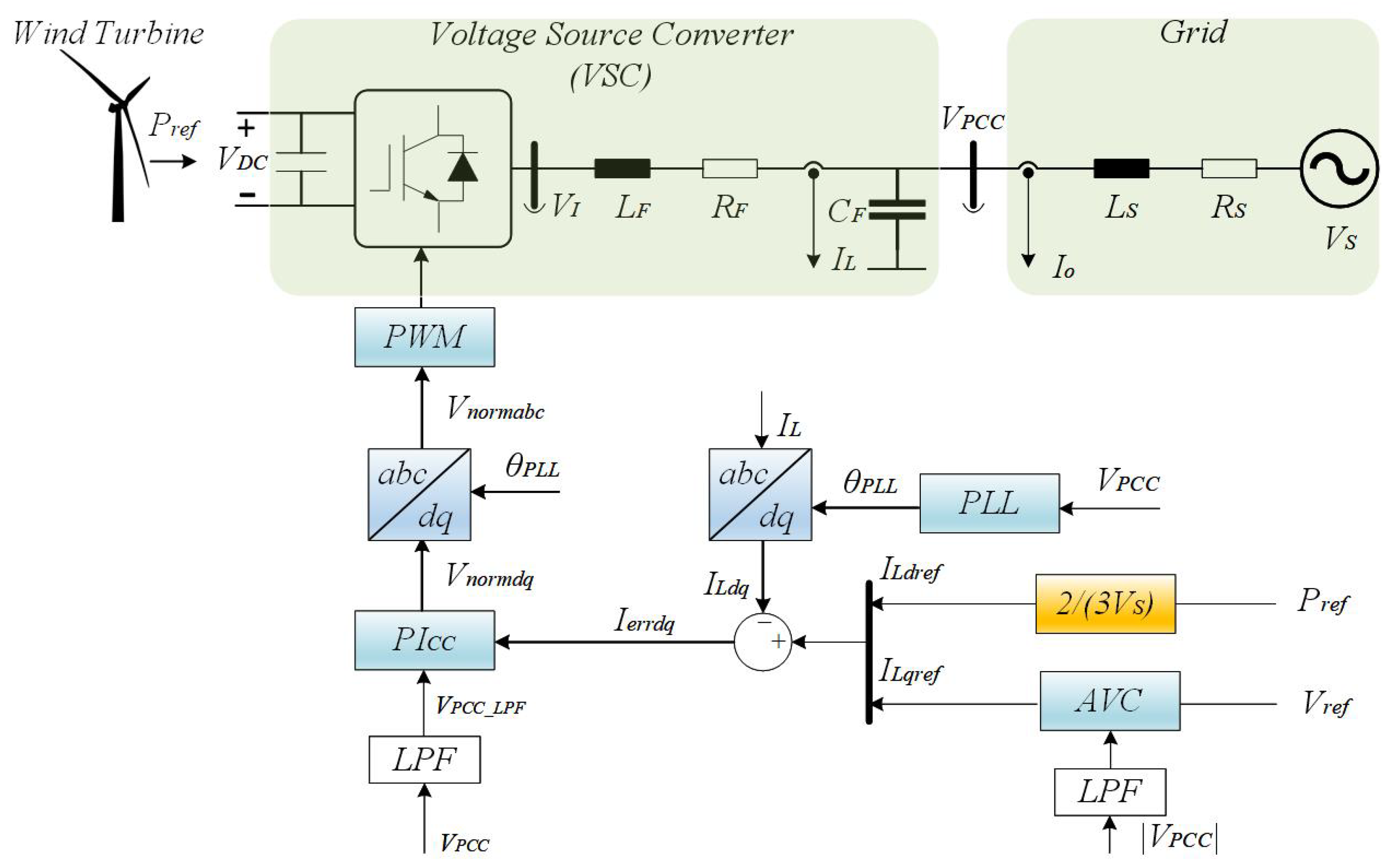
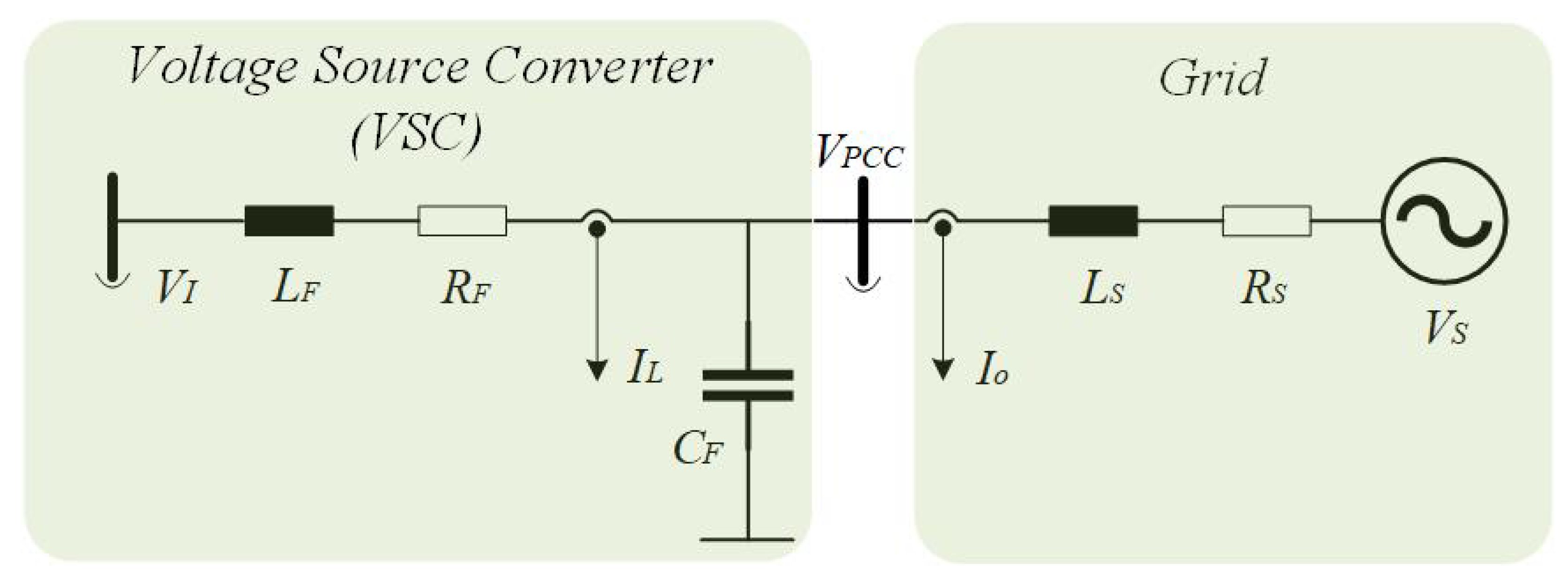
This study examines the grid-side converter of a wind turbine, utilizing a grid-following control structure as depicted in Figure 1. The philosophy is inherited from [22], incorporating a PLL to synchronize the converter with the grid. The DC link voltage of the inverter is assumed to be constant, and as the inverter is considered ideal, open-loop control is employed to track a specified reference value for active power. A new addition to this work is the AVC, which is used to regulate the voltage fed at the PCC of the VSC.

The dynamic behavior of the system is influenced by various nonlinear state equations that describe the control dynamics. These state equations create individual state-space models for each component, which when combined, form the overall nonlinear state-space model of the system. This is represented in (1):

$$\begin{array}{cc}\hfill & \dot{x}=Ax+R(x,u)\hfill \\ \hfill & y=S(x,u)\hfill \end{array}$$

(1)

where x represents the state variables of the system, u represents the system inputs, and y represents the system outputs. $R(x,u)$ and $S(x,u)$ describe the non-linear dependencies of the model.

2.1. dq Transformations

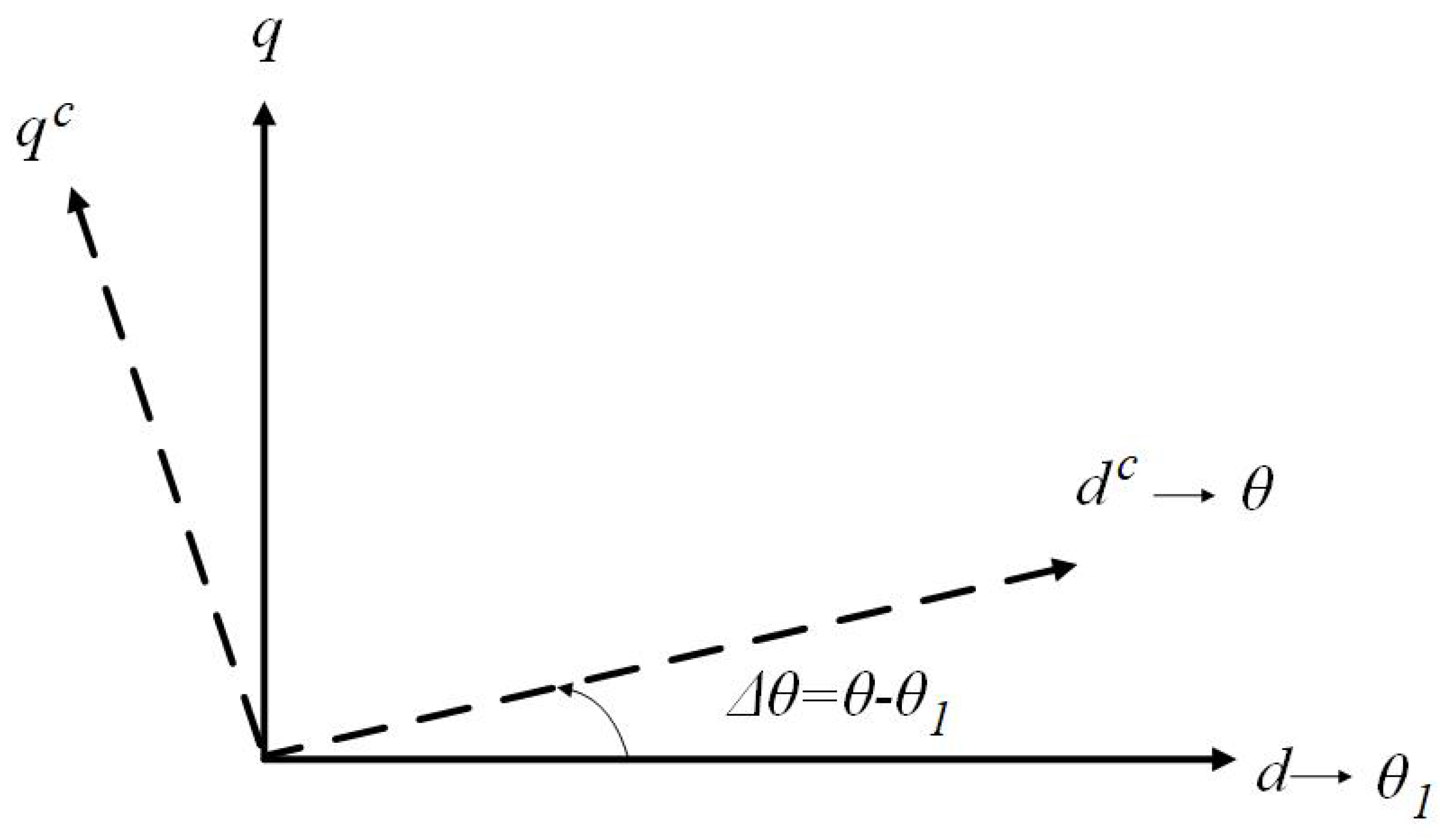
The control system in this model is implemented in the rotating dq frame, which is aligned with the phase angle of the PCC voltage $\theta$₁. However, the control system is also guided by the PLL output angle $\theta$. In dynamic conditions, these two angles have minimal errors [23]. To better understand the dynamics introduced by the PLL, two dq frames are defined: the grid dq frame, which is defined by $\theta$₁, and the control dq frame, which is defined by $\theta$. During steady-state operation, the PLL precisely follows the grid voltage angle, and the control dq frame is seamlessly synchronized with the grid dq frame. However, if there is a perturbation in the grid voltage, a phase shift $\Delta$$\theta$ between the two reference frames occurs and it takes some time for the PLL to lock onto the new grid voltage angle [24]. The output variables impacted by the control dq frame are the converter’s current $I_L$ and the PCC voltage $V_{PCC}$. In the following part of the paper, when these variables are in the control dq frame, they will be indicated by superscript c. The subscript 0 indicates the steady-state values of the corresponding variables. The relationship between the two dq frames is shown in Figure 2.

The equations of the transformation between the control and the grid dq frame derived from the Park and inverse Park transformation equations; they are given below:

$$\left[\begin{array}{c}{V}_{PCCd}^c\\ V_{PCCq}^c\end{array}\right]=\left[\begin{array}{cc}cos(\theta -{\theta }_1)& sin(\theta -{\theta }_1)\\ -sin(\theta -{\theta }_1)& cos(\theta -{\theta }_1)\end{array}\right]\left[\begin{array}{c}{V}_{PCCd}\\ V_{PCCq}\end{array}\right]$$

(2)

$$\left[\begin{array}{c}{I}_{Ld}^c\\ I_{Lq}^c\end{array}\right]=\left[\begin{array}{cc}cos(\theta -{\theta }_1)& sin(\theta -{\theta }_1)\\ -sin(\theta -{\theta }_1)& cos(\theta -{\theta }_1)\end{array}\right]\left[\begin{array}{c}{I}_{Ld}\\ I_{Lq}\end{array}\right]$$

(3)

After linearizing the equations of the transformation between the two dq frames, the small-signal equations are:

$$\Delta V_{PCCd}^c=\Delta V_{PCCd}+V_{PCCq,0}\Delta \theta$$

(4)

$$\Delta V_{PCCq}^c=\Delta V_{PCCq}-V_{PCCd,0}\Delta \theta$$

(5)

$$\Delta I_{Ld}^c=\Delta I_{Ld}+I_{Lq,0}\Delta \theta$$

(6)

$$\Delta I_{Lq}^c=\Delta I_{Lq}-I_{Ld,0}\Delta \theta$$

(7)

2.2. Phase-Locked Loop (PLL)

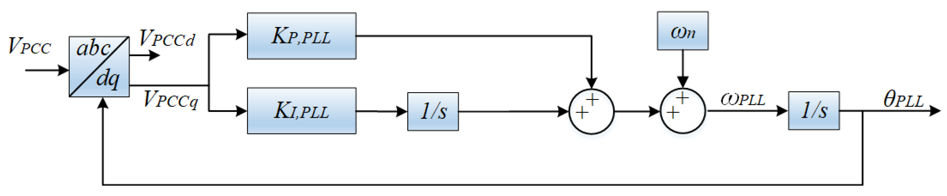
The control structure of the PLL is illustrated in Figure 3. The input to the PLL is the PCC voltage on the q-axis V_PCCq, and the output is the angular speed of the PCC voltage ω_PLL. The PI control regulates the voltage V_PCCq to zero, thus aligning the PCC voltage with the d-axis.

The state variables of the PLL are:

$$x_1=\left[\begin{array}{cc}{\theta }_{\mathrm{PLL}}& {\mathsf{\Phi }}_{\mathrm{PLL}}\end{array}\right]$$

(8)

where $\mathsf{\Phi }$_PLL=$\int V_{PCCq}^{c}dt$.

The differential equations of the PLL are the following:

$${\dot{\theta }}_{\mathrm{PLL}}=K_{\mathrm{I},\mathrm{PLL}}{\mathsf{\Phi }}_{\mathrm{PLL}}+K_{\mathrm{P},\mathrm{PLL}}{V}_{PCCq}^c+{\omega }_{\mathrm{n}}$$

(9)

$${\dot{\mathsf{\Phi }}}_{\mathrm{PLL}}=V_{PCCq}^c$$

(10)

2.3. Current Controller

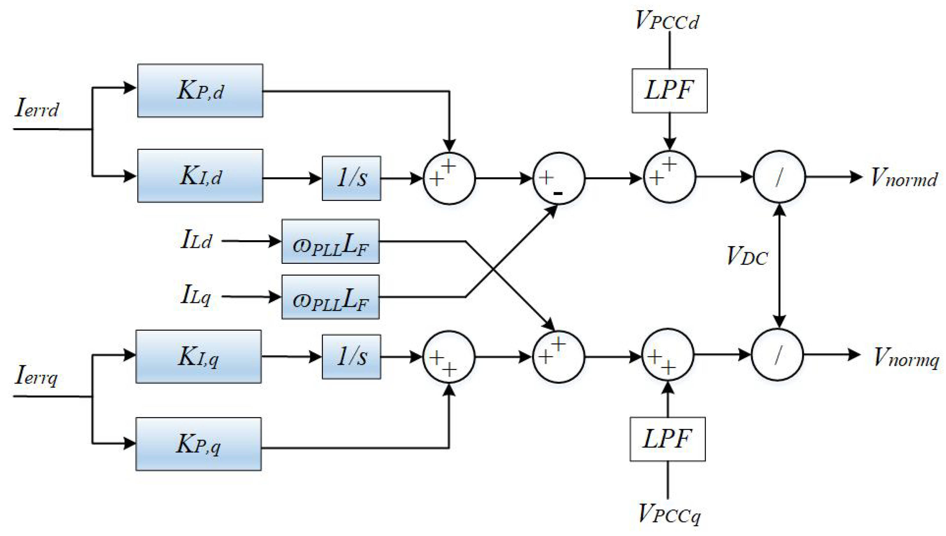
The current control loop is shown in Figure 4 along with the feedforward voltage. As shown in Figure 4, it generates a normalized voltage reference in order to control the converter current. The corresponding algebraic equations of the current controller’s output are given below:

$$\begin{array}{c}\hfill V_{\mathrm{normd}}=\frac{1}{V_{\mathrm{DC}}}(V_{\mathrm{PCCd},\mathrm{LPF}}-{\omega }_{\mathrm{PLL}}{L}_{\mathrm{F}}{I}_{Lq}^c+K_{\mathrm{P},\mathrm{d}}{I}_{\mathrm{e}\mathrm{r}\mathrm{r}\mathrm{d}}+K_{\mathrm{I},\mathrm{d}}{q}_{\mathrm{e}\mathrm{r}\mathrm{r}\mathrm{d}})\end{array}$$

(11)

$$\begin{array}{c}\hfill V_{\mathrm{normq}}=\frac{1}{V_{\mathrm{DC}}}(V_{\mathrm{PCCq},\mathrm{LPF}}+{\omega }_{\mathrm{PLL}}{L}_{\mathrm{F}}{I}_{Ld}^c+K_{\mathrm{P},\mathrm{q}}{I}_{\mathrm{e}\mathrm{r}\mathrm{r}\mathrm{q}}+K_{\mathrm{I},\mathrm{q}}{q}_{\mathrm{e}\mathrm{r}\mathrm{r}\mathrm{q}})\end{array}$$

(12)

where q_errdq denotes the current controller’s integrators.

The current controller takes as input the error current, which represents the difference between the desired dq-axis current $I_{\mathrm{Ldref}}$ and the actual converter current $I_{\mathrm{Ldq}}$. The reference q-axis current is determined by the AVC control loop, which will be discussed in the following subsection. The reference d-axis current is obtained from the injected active power reference, as shown in (13), where $|V_{PCC}|$ is the magnitude of the voltage at PCC, which is discussed in Section 2.4:

$$I_{\mathrm{Ldref}}=\frac{2}{3}\frac{P_{\mathrm{ref}}}{|V_{PCC}|}$$

(13)

The state variables of the current controller—including the low-pass filters at the feed-forward voltage—are:

$$x_2=\left[\begin{array}{cccc}{q}_{\mathrm{errd}}& q_{\mathrm{errq}}& V_{\mathrm{PCCd},\mathrm{LPF}}& V_{\mathrm{PCCq},\mathrm{LPF}}\end{array}\right]$$

(14)

The differential equations of the current controller are shown in (15)–(18):

$${\dot{q}}_{\mathrm{errd}}=I_{\mathrm{Ldref}}-I_{Ld}^c$$

(15)

$${\dot{q}}_{\mathrm{errq}}=I_{\mathrm{Lqref}}-I_{Lq}^c$$

(16)

$${\dot{V}}_{\mathrm{PCCd},\mathrm{LPF}}=-{\omega }_{\mathrm{FF},\mathrm{LPF}}{V}_{\mathrm{PCCd},\mathrm{LPF}}+{\omega }_{\mathrm{FF},\mathrm{LPF}}{V}_{PCCd}^c$$

(17)

$${\dot{V}}_{\mathrm{PCCq},\mathrm{LPF}}=-{\omega }_{\mathrm{FF},\mathrm{LPF}}{V}_{\mathrm{PCCq},\mathrm{LPF}}+{\omega }_{\mathrm{FF},\mathrm{LPF}}{V}_{PCCq}^c$$

(18)

where ${\omega }_{\mathrm{FF},\mathrm{LPF}}$ is the cutoff frequency of the low-pass filter at the feedforward voltage.

2.4. Alternating Voltage Controller (AVC)

The outer control loop is responsible for the generation of the q-axis current reference (reactive current) and keeps the AC voltage fixed. The AVC is utilized to regulate the voltage at the point of common coupling, and it is implemented by using the classical PI control. It is shown in Figure 5.

According to Figure 5, the voltage magnitude at the PCC is regulated to the desired reference voltage after it is filtered, in order, e.g., to exclude unwanted 2nd-order harmonics, as explained in the introduction. The voltage magnitude will be symbolized as $V_{\mathrm{M}}$ and it is equal to:

$$V_{\mathrm{M}}=\sqrt{{V_{PCCd}}^2+{V_{PCCq}}^2}$$

(19)

Therefore, the reference current in the q-axis is derived by the following formula:

$$I_{\mathrm{L}\mathrm{q}\mathrm{r}\mathrm{e}\mathrm{f}}=-(K_{\mathrm{P},\mathrm{a}}(V_{\mathrm{P}\mathrm{C}\mathrm{C}\mathrm{r}\mathrm{e}\mathrm{f}}-V_{\mathrm{M},\mathrm{L}\mathrm{P}\mathrm{F}})+K_{\mathrm{I},\mathrm{a}}{q}_{\mathrm{e}\mathrm{r}\mathrm{r}\mathrm{a}\mathrm{c}})$$

(20)

where q_errac represents the integrator of AVC.

The state variables of the AVC are:

$$x_3=\left[\begin{array}{cc}{q}_{\mathrm{e}\mathrm{r}\mathrm{r}\mathrm{a}\mathrm{c}}& V_{\mathrm{M},\mathrm{L}\mathrm{P}\mathrm{F}}\end{array}\right]$$

(21)

The differential equations of the AVC are the following:

$${\dot{q}}_{\mathrm{e}\mathrm{r}\mathrm{r}\mathrm{a}\mathrm{c}}=V_{\mathrm{P}\mathrm{C}\mathrm{C}\mathrm{r}\mathrm{e}\mathrm{f}}-V_{\mathrm{M},\mathrm{L}\mathrm{P}\mathrm{F}}$$

(22)

$${\dot{V}}_{\mathrm{M},\mathrm{L}\mathrm{P}\mathrm{F}}=-{\omega }_{\mathrm{A}\mathrm{V}\mathrm{C},\mathrm{L}\mathrm{P}\mathrm{F}}{V}_{\mathrm{M},\mathrm{L}\mathrm{P}\mathrm{F}}+{\omega }_{\mathrm{A}\mathrm{V}\mathrm{C},\mathrm{L}\mathrm{P}\mathrm{F}}{V}_{\mathrm{M}}$$

(23)

where ${\omega }_{\mathrm{A}\mathrm{V}\mathrm{C},\mathrm{L}\mathrm{P}\mathrm{F}}$ is the cutoff frequency of the low-pass filter at $V_{\mathrm{M}}$.

2.5. Time Delay

Time delay is a significant aspect of digital control systems, and it is considered in this analysis. The delay is modeled using a 3rd-order Padé approximation, which approximates the delay in the system by using the transfer function provided in (24):

$$e^{-{\mathrm{T}}_{\mathrm{d}}\mathrm{s}}=\frac{\left(b_0+b_1{T}_{\mathrm{d}}s+\dots +b_{\mathrm{l}}{\left(T_{\mathrm{d}}s\right)}^{\mathrm{l}}\right)}{\left(a_0+a_1{T}_{\mathrm{d}}s+\dots +a_{\mathrm{k}}{\left(T_{\mathrm{d}}s\right)}^{\mathrm{k}}\right)}$$

(24)

where l and k are the order of Padé approximation,

$$a_{\mathrm{j}}=\frac{\left(l+k-j\right)!k!}{j!\left(k-j\right)!},j=0,\dots ,k$$

(25)

and

$$b_{\mathrm{i}}={\left(-1\right)}^{\mathrm{i}}\frac{\left(l+k-i\right)!l!}{i!\left(l-i\right)!},i=0,\dots ,l$$

(26)

The delay time, $T_{\mathrm{d}}$, is typically set to be $1.5$ times the sampling period.

The state variables that describe the time delay are as follows:

$$x_4=\left[\begin{array}{cccccc}{x}_{\mathrm{d}\mathrm{e}\mathrm{l},1\mathrm{d}}& x_{d\mathrm{e}\mathrm{l},2\mathrm{d}}& x_{\mathrm{d}\mathrm{e}\mathrm{l},3\mathrm{d}}& x_{del,1q}& x_{\mathrm{d}\mathrm{e}\mathrm{l},2\mathrm{q}}& x_{\mathrm{d}\mathrm{e}\mathrm{l},3\mathrm{q}}\end{array}\right]$$

(27)

The differential equations of the digital time delay—where each equation can be used in both the d- and q-frame—are the following:

$${\dot{x}}_{\mathrm{d}\mathrm{e}\mathrm{l},1\mathrm{d}\mathrm{q}}=0x_{\mathrm{d}\mathrm{e}\mathrm{l},1\mathrm{d}\mathrm{q}}+1x_{\mathrm{d}\mathrm{e}\mathrm{l},2\mathrm{d}\mathrm{q}}+0x_{\mathrm{d}\mathrm{e}\mathrm{l},3\mathrm{d}\mathrm{q}}$$

(28)

$${\dot{x}}_{\mathrm{d}\mathrm{e}\mathrm{l},2\mathrm{d}\mathrm{q}}=0x_{\mathrm{d}\mathrm{e}\mathrm{l},1\mathrm{d}\mathrm{q}}+0x_{\mathrm{d}\mathrm{e}\mathrm{l},2\mathrm{d}\mathrm{q}}+1x_{\mathrm{d}\mathrm{e}\mathrm{l},3\mathrm{d}\mathrm{q}}$$

(29)

$${\dot{x}}_{\mathrm{d}\mathrm{e}\mathrm{l},3\mathrm{d}\mathrm{q}}=-\frac{120}{T_d^3}{x}_{\mathrm{d}\mathrm{e}\mathrm{l},1\mathrm{d}\mathrm{q}}-\frac{60}{T_d^2}{x}_{\mathrm{d}\mathrm{e}\mathrm{l},2\mathrm{d}\mathrm{q}}-\frac{12}{T_d^1}{x}_{\mathrm{d}\mathrm{e}\mathrm{l},3\mathrm{d}\mathrm{q}}+V_{\mathrm{n}\mathrm{o}\mathrm{r}\mathrm{m}\mathrm{d}\mathrm{q}}$$

(30)

2.6. LC Filter and Grid-Side Impedance

An LC filter is included in the model—as shown in Figure 6—to attenuate the high harmonics that are derived from the converter as well as the modulation harmonics. The dynamics of the grid impedance are also included in the state-space subsystem, and the corresponding state variables are shown below:

$$x_5=\left[\begin{array}{cccccc}{I}_{Ld}^c& I_{Lq}^c& V_{\mathrm{P}\mathrm{C}\mathrm{C}\mathrm{d}}& V_{\mathrm{P}\mathrm{C}\mathrm{C}\mathrm{q}}& I_{\mathrm{o}\mathrm{d}}& I_{\mathrm{o}\mathrm{q}}\end{array}\right]$$

(31)

The Padé approximation from the time delay is used to obtain the VSC bridge voltage $V_I$, as $V_I$ is the output of the time delay state-space subsystem:

$$\begin{array}{c}\hfill V_{\mathrm{I}\mathrm{d}}=V_{\mathrm{D}\mathrm{C}}(\frac{240}{T_d^3}{x}_{\mathrm{d}\mathrm{e}\mathrm{l},1\mathrm{d}}+0x_{\mathrm{d}\mathrm{e}\mathrm{l},2\mathrm{d}}+\frac{24}{T_d^1}{x}_{\mathrm{d}\mathrm{e}\mathrm{l},3\mathrm{d}}-V_{\mathrm{n}\mathrm{o}\mathrm{r}\mathrm{m}\mathrm{d}})\end{array}$$

(32)

$$\begin{array}{c}\hfill V_{\mathrm{I}\mathrm{q}}=V_{\mathrm{D}\mathrm{C}}(\frac{240}{T_d^3}{x}_{\mathrm{d}\mathrm{e}\mathrm{l},1\mathrm{q}}+0x_{\mathrm{d}\mathrm{e}\mathrm{l},2\mathrm{q}}+\frac{24}{T_d^1}{x}_{\mathrm{d}\mathrm{e}\mathrm{l},3\mathrm{q}}-V_{\mathrm{n}\mathrm{o}\mathrm{r}\mathrm{m}\mathrm{q}})\end{array}$$

(33)

The state equations of the convert current $I_L$, the voltage at PCC $V_{PCC}$, and the output current $I_o$ are shown in (34)–(39):

$${\dot{I}}_{Ld}^c=-\frac{R_F}{L_F}{I}_{Ld}^c+\left(-\frac{1}{L_F}{V}_{PCCd}^c\right)+{\omega }_{\mathrm{P}\mathrm{L}\mathrm{L}}{I}_{Lq}^c+\frac{1}{L_F}{V}_{\mathrm{I}\mathrm{d}}$$

(34)

$${\dot{I}}_{Lq}^c=-\frac{R_F}{L_F}{I}_{Lq}^c+\left(-\frac{1}{L_F}{V}_{PCCq}^c\right)-{\omega }_{\mathrm{P}\mathrm{L}\mathrm{L}}{I}_{Ld}^c+\frac{1}{L_F}{V}_{\mathrm{I}\mathrm{q}}$$

(35)

$${\dot{V}}_{\mathrm{P}\mathrm{C}\mathrm{C}\mathrm{d}}=\frac{1}{C_F}{I}_{Ld}+\left(-\frac{1}{C_F}{I}_{od}\right)+{\omega }_n{V}_{PCCq}$$

(36)

$${\dot{V}}_{\mathrm{P}\mathrm{C}\mathrm{C}\mathrm{q}}=\frac{1}{C_F}{I}_{Lq}+\left(-\frac{1}{C_F}{I}_{oq}\right)-{\omega }_n{V}_{PCCd}$$

(37)

$${\dot{I}}_{\mathrm{o}\mathrm{d}}=\frac{1}{L_S}{V}_{PCCd}+\left(-\frac{R_S}{L_S}{I}_{od}\right)+\left(-\frac{1}{L_S}{V}_{Sd}\right)+{\omega }_n{I}_{oq}$$

(38)

$${\dot{I}}_{\mathrm{o}\mathrm{q}}=\frac{1}{L_S}{V}_{PCCq}+\left(-\frac{R_S}{L_S}{I}_{oq}\right)+\left(-\frac{1}{L_S}{V}_{Sq}\right)-{\omega }_n{I}_{od}$$

(39)

3. Small-Signal Stability Analysis Assessment Based on Eigenvalue Analysis

Subsynchronous and near-synchronous oscillations of the fundamental frequency are the most common cases of instability in small-signal models based on the grid-following control. A linearized state-space model is required in order to assess the small-signal instability of the system. The linearization is implemented around the equilibrium points of the overall state-space model of the system, and this linear approximation is shown in (40):

$$\dot{x}=Ax,$$

(40)

where A is the Jacobian matrix derived from the partial derivatives of the system at the equilibrium points.

3.1. Equilibrium Points Computation

The equilibrium states of the state-space model consist of the voltage at PCC $V_{PCC,0}$ and the inductor current $I_{L,0}$—both in the dq reference frame—and they are used in (4)–(7).

As $V_{PCCq}$ is regulated to zero at the PLL, the corresponding equilibrium state $V_{PCCq,0}$ is equal to zero. Given that, as well as the definition of $V_M$ in Section 2.4, $V_{PCCd,0}$ is equal to $V_{PCCref}$. The equilibrium state of the inductor current at d-axis $I_{Ld,0}$ is equal to $I_{Ldref}$. The equilibrium state of the inductor current at q-axis $I_{Lq,0}$ is derived by Kirchhoff’s voltage law (KVL) on the grid side:

$$V_{\mathrm{P}\mathrm{C}\mathrm{C}\mathrm{d},0}=V_{\mathrm{S}\mathrm{d},0}+R_{\mathrm{S}}{I}_{od,0}-{\omega }_n{L}_S{I}_{oq,0}$$

(41)

In (42) and (43), the relationship between the steady-state converter and the output current—in the d- and q-axis—is shown:

$$I_{\mathrm{o}\mathrm{d},0}=I_{\mathrm{L}\mathrm{d},0}=I_{Ldref}$$

(42)

$$I_{\mathrm{o}\mathrm{q},0}=I_{\mathrm{L}\mathrm{q},0}-{\omega }_n{V}_{\mathrm{P}\mathrm{C}\mathrm{C}\mathrm{d},0}{C}_F$$

(43)

The grid voltage on the d-axis $V_{Sd,0}$ is given by the following formula:

$$V_{Sd,0}=\left|V_{Sabc}\right|cos\delta$$

(44)

where $\delta$ is the grid angle with respect to the capacitor voltage of each converter. This angle can be estimated if we consider the injected active power to the grid by the converter in the abc frame:

$$P=\frac{3}{2}\frac{|V_{PCCabc}\left|\right|V_{Sabc}|sin\left(\delta \right)}{{\omega }_n{L}_S}$$

(45)

As already mentioned, the control is oriented to the d-axis; therefore, the active power in the dq frame can be calculated by considering only the variables of the d-axis:

$$P=\frac{3}{2}{V}_{PCCd}{I}_{od}=\frac{3}{2}\left|V_{PCCabc}\right|I_{od}$$

(46)

Therefore, angle $\delta$ can now be estimated by using (45) and (46) and the following formula is obtained:

$$cos\delta =\sqrt{1-{\left(\frac{{\omega }_n{L}_S{I}_{od}}{|V_{Sabc}|}\right)}^2}$$

(47)

So, taking into account (42), (43), (44), and (47) into (41), the equilibrium state of the inductor current in the q-axis is obtained in (48):

$$I_{Lq,0}=\frac{\sqrt{|V_{Sabc}{|}^2-{\left({\omega }_n{L}_S{I}_{Ldref}\right)}^2}+R_S{I}_{Ldref}-V_{PCCref}\left(1-{\left({\omega }_n\right)}^2{L}_{S}C\right)}{{\omega }_n{L}_S}$$

(48)

After the calculation of the equilibrium points is completed, the state-space model can be linearized around them.

3.2. Grid strength and Eigenvalue-Based Stability Analysis

The strength of a power grid is determined by the short circuit ratio (SCR), which represents the ratio of the maximum short-circuit power $S_{SC}$ at PCC to the rated power $S_N$ of the voltage source converter (VSC). The SCR is given by:

$$SCR=\frac{S_{SC}}{S_N}=\frac{\frac{3}{2}\frac{{\left(V_S\right)}^2}{|Z_S|}}{\frac{3}{2}{V}_{PCC}{I}_{Ldref}}$$

(49)

Therefore, a grid impedance impacts the grid strength, as its increase leads to the decrease of the short-circuit power.

An eigenvalue analysis is performed on the small-signal model using the system and control parameters listed in

Table A1. System and default control parameters.

	Description	Value
VS	Grid Phase Voltage (peak value)	311 V
fn	Rated Frequency	50 Hz
VDC	DC Link Voltage Reference	800 V
LF	Filter Inductance	5 mH
RF	Filter Resistance	0.1 $\Omega$
CF	Filter Capacitance	10 $\mathsf{\mu }$F
fsw	Switching Frequency	20 kHz
fS	Sampling Frequency	20 kHz
VPCCref	Reference PCC Voltage (peak value)	280 V
Pref	Nominal Active Power	30 kW
ωFF,LPF	Cutoff Frequency of Feedforward Voltage	100 rad/s
KI0	Default Integral Gain of Current Control	666.7
KP0	Default Proportional Gain of Current Control	33.3
KI,PLL0	Default Integral Gain of PLL	0
KP,PLL0	Default Proportional Gain of PLL	0.1637
KI,a0	Default Integral Gain of AVC	100
KP,a0	Default Proportional Gain of AVC	0

. The goal of the default PI’s current controller is to have a closed loop current bandwidth of around 1/20 of the switching frequency. A low PLL bandwidth is chosen—equal to $7.27$ Hz—in order to attenuate the effect of a possible distortion on the PLL output signals by high-order harmonics. The grid inductance $L_S$ is specified by (49), while the grid resistance $R_S$ is assumed to be zero in this analysis. The AVC design is related to $L_S$ and that impacts the AVC bandwidth in case the grid strength changes. Moreover, the response time of the inner-current loop is much faster than the outer-AVC loop, so AVC’s bandwidth should be much smaller that the current controller’s bandwidth.

Three different cases of the cutoff frequency of the AVC’s low-pass filter $f_{\mathrm{AVC},\mathrm{LPF}}$ are selected for the eigenvalue analysis; in fact, $f_{\mathrm{AVC},\mathrm{LPF}}$ is equal to 20 Hz, 50 Hz (equal to the nominal frequency), and 100 Hz, which is the upper limit of the cutoff frequency, as the goal of the low-pass filter is to extract the 2nd-order harmonics. The eigenvalue sensitivity analysis is then carried out to determine the small-signal stability and the effect of the controllers. This analysis involves altering the control parameters of the system’s control structures and measuring the correlation between instability and the magnitude of the changes. The equilibrium points of the state-space model are re-estimated in each variation of the controller under test until the system reaches instability. Instability is identified when the real part of the complex eigenvalue obtains a positive value, meaning that the damping becomes negative. In that way, a new eigenvalue analysis is carried out each time a parameter is swept, which will finally lead to an eigenvalue trace that shows the stability trend of the corresponding control parameter.

The weak grid case scenario is studied first when the SCR is equal to 1.5. The grid inductance $L_S$ is equal to $10.3$ mH, the current controller’s bandwidth is equal to 292 Hz, and the AVC bandwidth is equal to $51.31$ Hz. The PLL proportional gain $K_{P,PLL}$ of the VSC system is adjusted multiple times, starting from 0.1 times its default value $K_{P,PLL0}$ (deep blue) and increasing up to 10 times (deep red) in order to identify the specific PLL bandwidths that cause instability in the system. The goal of this analysis is to determine the range of $K_{P,PLL}$ values that result in a stable system operation. The results are shown in Figure 7, where the critical PLL proportional gain $K_{P,PLLcr}$—with the corresponding PLL bandwidth—is obtained for the $f_{\mathrm{AVC},\mathrm{LPF}}$ under study. The oscillation frequency $F_{cr}$ of the critical mode of instability is also shown.

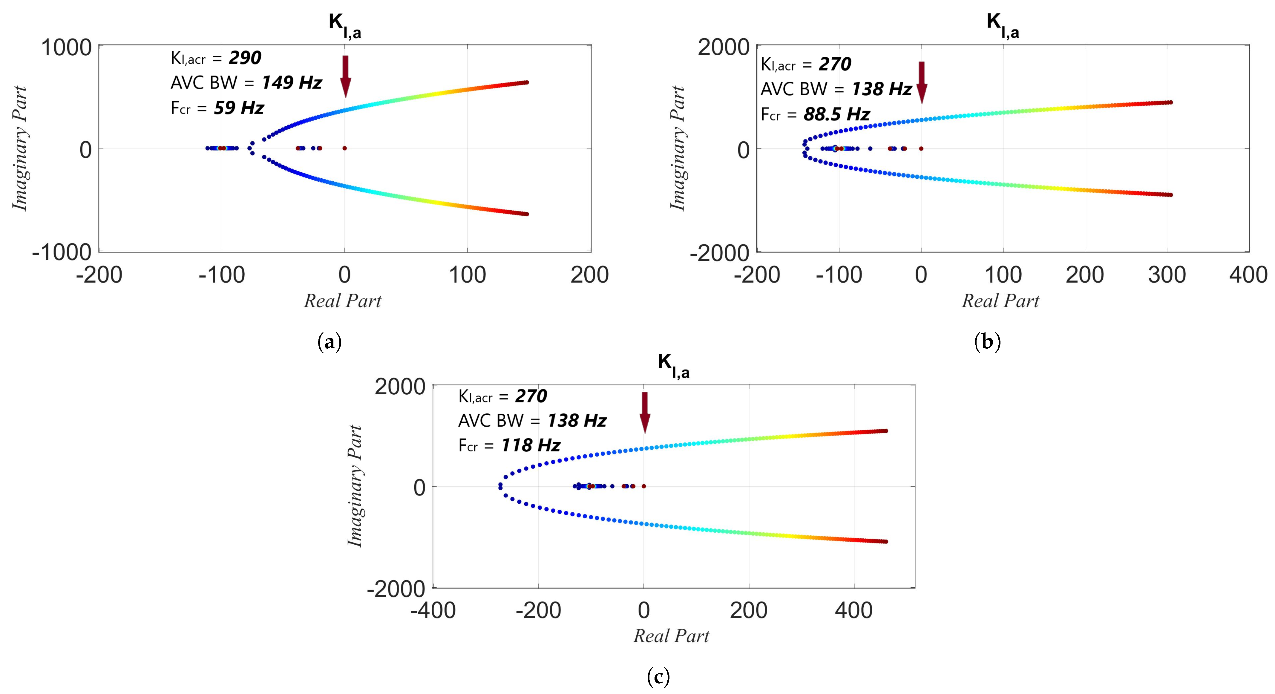
The same procedure is used in order to identify the critical AVC bandwidth where the system becomes unstable. The default AVC integral gain $K_{I,a0}$ of the VSC of the system varies from 0.1 (deep blue) to 10 (deep red) times. The results are shown in Figure 8, where the critical AVC integral gain $K_{I,acr}$—with the corresponding AVC bandwidth—is identified for the corresponding $f_{\mathrm{AVC},\mathrm{LPF}}$. The oscillation frequency $F_{cr}$ of the critical mode of instability is also shown. Based on these results, the instability in the weak grid case occurs when the AVC bandwidth obtains a value close to 1/2 of the current controller’s bandwidth.

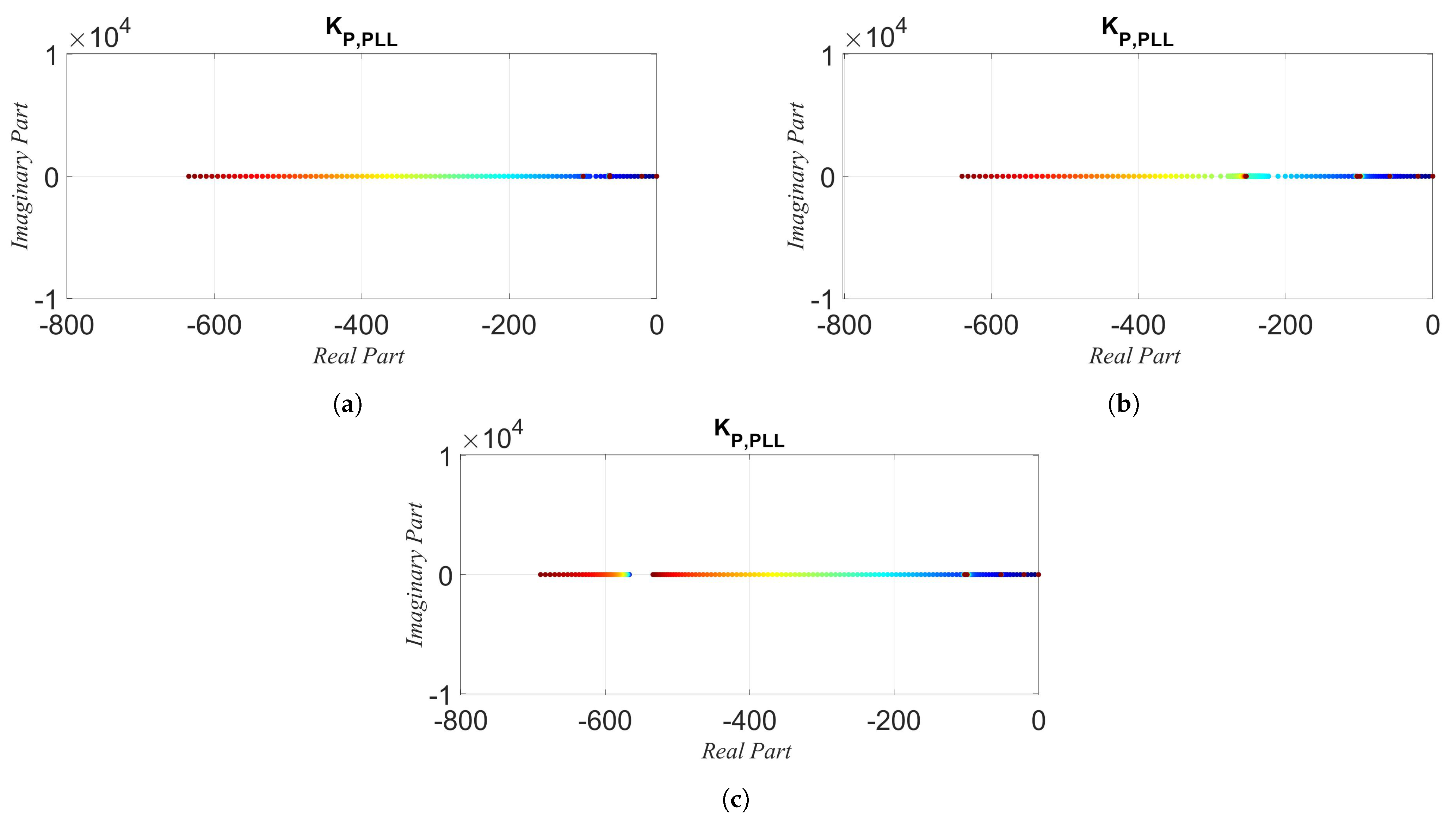
Then a strong grid case scenario is studied, with an SCR equal to 10. The grid inductance $L_S$ is equal to $1.5$ mH, the current controller’s bandwidth is equal to 953 Hz and the AVC bandwidth is equal to $7.7$ Hz. The PLL proportional gain $K_{P,PLL0}$ of the VSC in the system varies from 0.1 (deep blue) to 10 (deep red) times, in order to identify if there are any critical PLL bandwidths where the system becomes unstable. The results are shown in Figure 9, where no critical PLL bandwidths are identified for the corresponding $f_{\mathrm{AVC},\mathrm{LPF}}$.

In order to identify the critical AVC bandwidth where the system becomes unstable, $K_{I,a0}$ varies from 1 (deep blue) to 200 (deep red) times. The results are shown in Figure 10, where the critical AVC integral gain $K_{I,acr}$—with the corresponding AVC bandwidth—is identified for the corresponding $f_{\mathrm{AVC},\mathrm{LPF}}$. The oscillation frequency $F_{cr}$ of the critical mode of instability is also shown. Based on these results, the instability in the strong grid case occurs when the AVC bandwidth obtains a relatively high value, which is a bit higher than 2/3 of the current controller’s bandwidth, with a tendency to decrease as $f_{\mathrm{AVC},\mathrm{LPF}}$ is increased.

4. Stability Regions of PLL and AVC Depending on the AVC’s LPF Cutoff Frequency

The small-signal stability analysis assessment, which was analyzed in Section 3, provided the eigenvalue analysis trends of the PLL and AVC bandwidth for specific values of AVC’s LPF cutoff frequency $f_{\mathrm{AVC},\mathrm{LPF}}$. The accuracy of the small-signal analysis—which is later validated by the time domain simulation results—allows the identification of stability regions for the above-mentioned control loops when $f_{\mathrm{AVC},\mathrm{LPF}}$ varies.

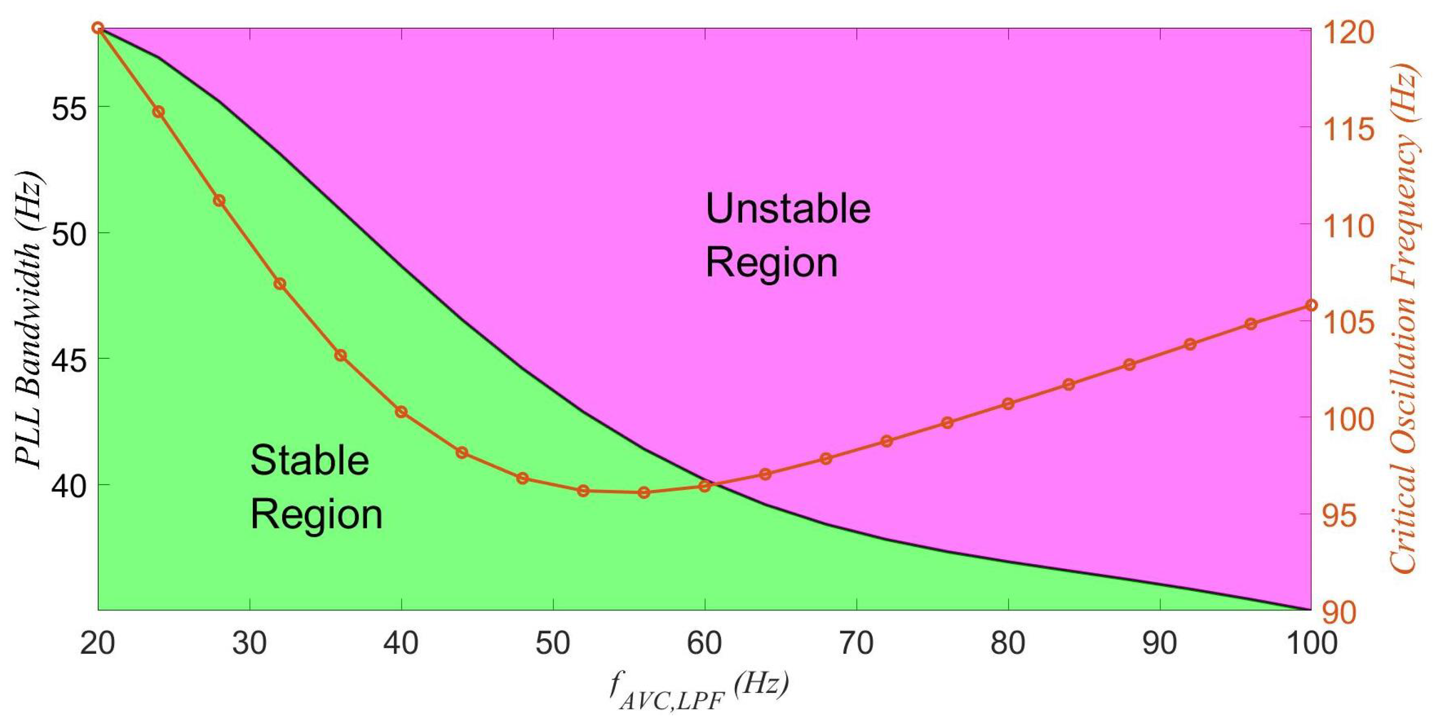
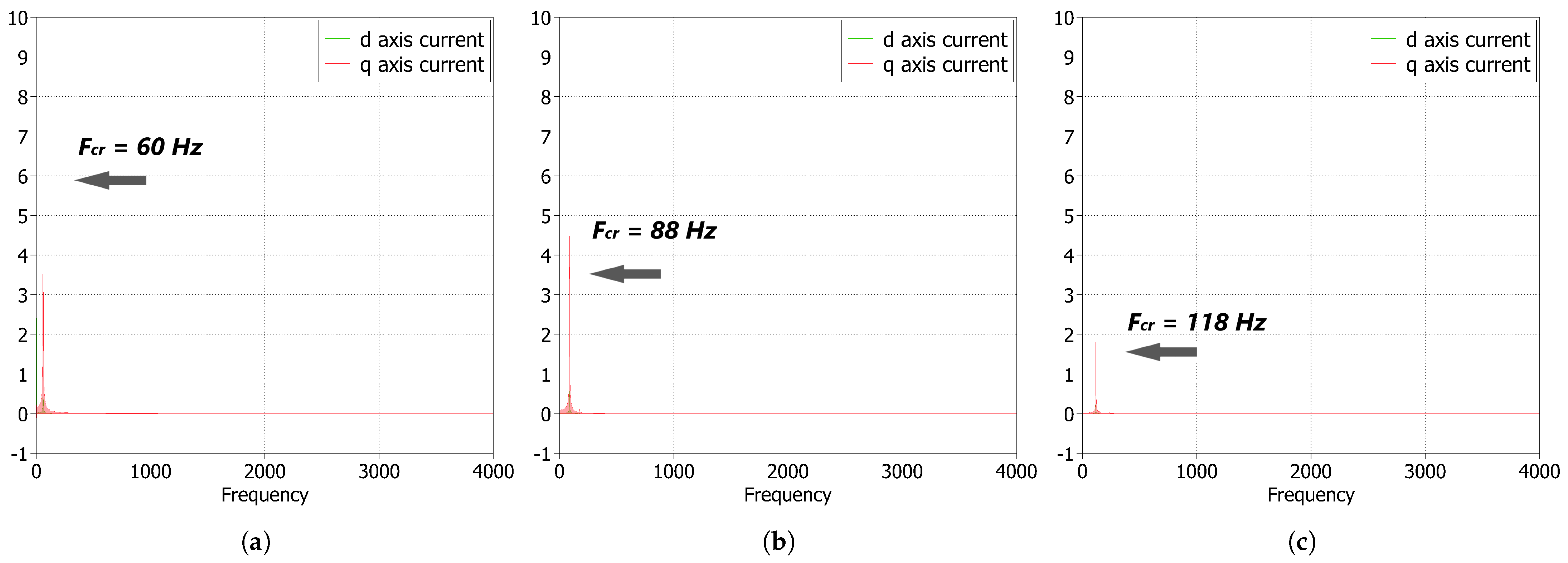
In the weak grid case scenario (SCR = 1.5), the stability region of the PLL bandwidth is shown in Figure 11. According to these graphs, the critical PLL bandwidth is equal to 58.2 Hz for $f_{\mathrm{AVC},\mathrm{LPF}}$ equal to 20 Hz. The critical PLL bandwidth drops rapidly to 40 Hz when the cutoff frequency varies from 20 to 60 Hz. Then, the critical PLL bandwidth drops more smoothly, reaching a value of 34.93 Hz when $f_{\mathrm{AVC},\mathrm{LPF}}$ varies from 60 to 100 Hz. The oscillation frequency that corresponds to the critical PLL bandwidth is equal to 120.16 Hz for $f_{\mathrm{AVC},\mathrm{LPF}}$ equal to 20 Hz. When $f_{\mathrm{AVC},\mathrm{LPF}}$ varies from 20 to 56 Hz, the oscillation frequency drops to 96.13 Hz; however, this frequency rises to 105.84 Hz when $f_{\mathrm{AVC},\mathrm{LPF}}$ varies from 56 to 100 Hz.

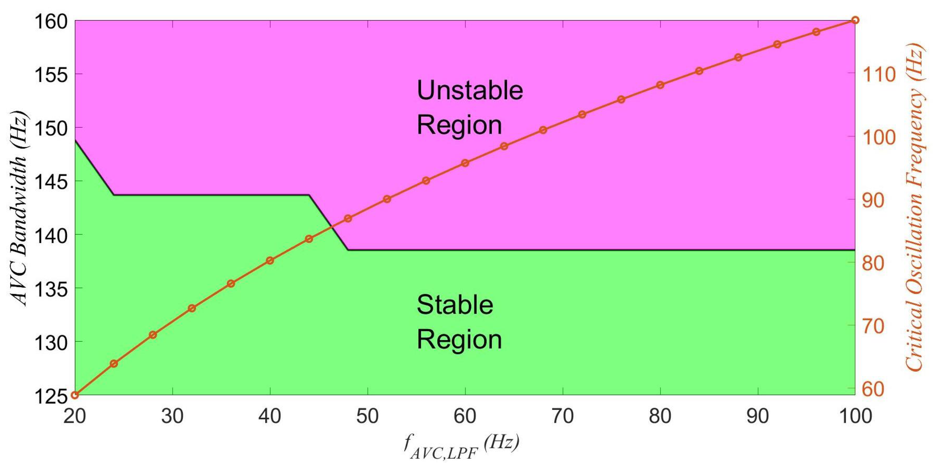
Similarly, the stability region of the AVC bandwidth in the weak grid case is shown in Figure 12. The critical AVC bandwidth is equal to 149 Hz for $f_{\mathrm{AVC},\mathrm{LPF}}$ that is equal to 20 Hz. The critical AVC bandwidth drops to 143 Hz when the cutoff frequency varies from 24 to 44 Hz, and then obtains a value equal to 138 Hz until $f_{\mathrm{AVC},\mathrm{LPF}}$ is equal to 100 Hz. Therefore, AVC’s critical bandwidth is not impacted by the variations of $f_{\mathrm{AVC},\mathrm{LPF}}$. The oscillation frequency that corresponds to the critical AVC bandwidth is equal to 58.9 Hz for $f_{\mathrm{AVC},\mathrm{LPF}}$ that is equal to 20 Hz. When $f_{\mathrm{AVC},\mathrm{LPF}}$ varies from 20 to 100 Hz, the oscillation frequency increases to 118.4 Hz.

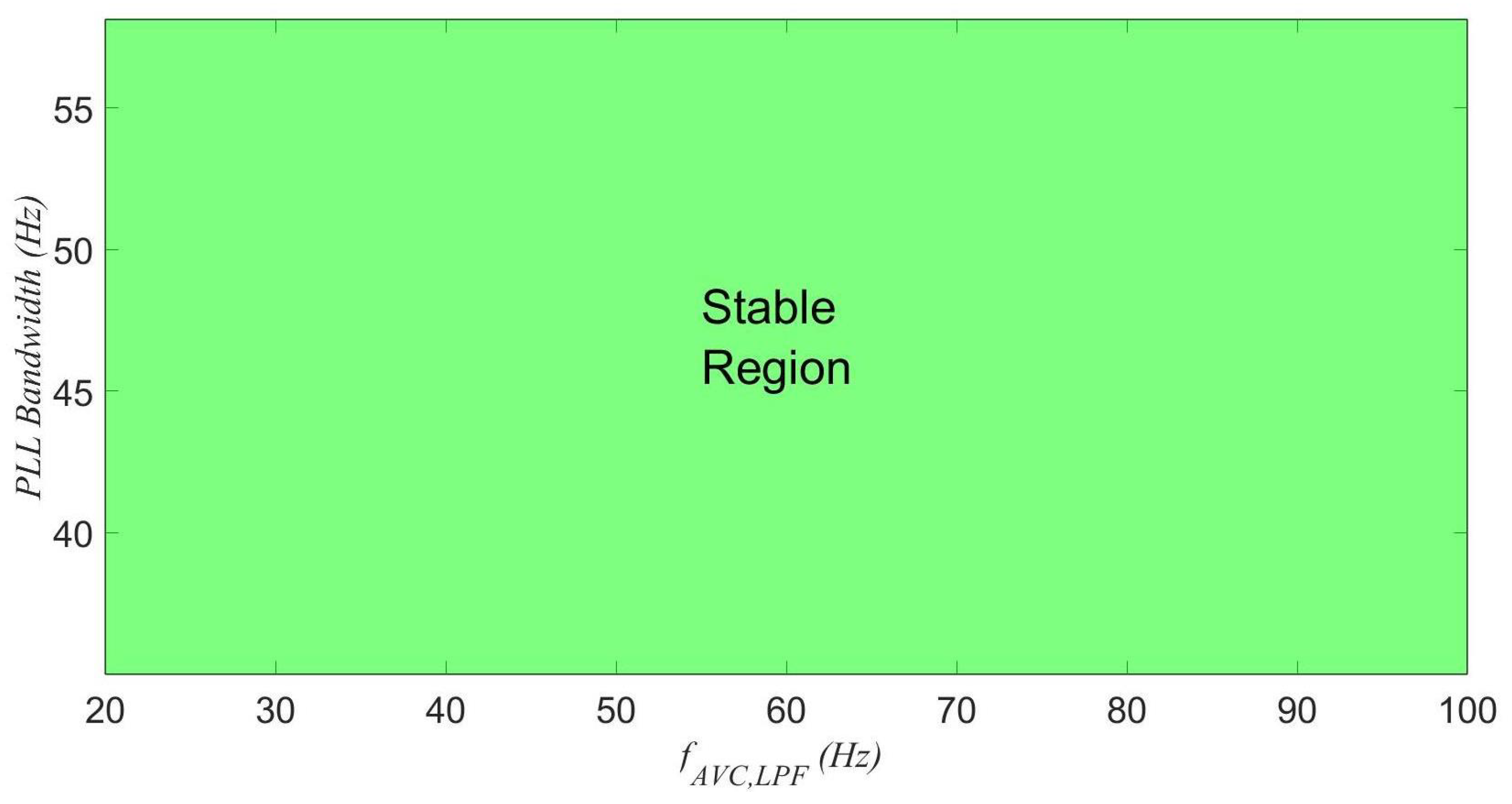
In the strong grid case scenario (SCR = 10), the stability region of the PLL is shown in Figure 13. According to this result, the PLL bandwidth does not impact the system’s stability when the grid is strong, as also shown in the corresponding small-signal stability assessment in the previous section. Therefore, the instability region is stable, and as a result, there are no oscillation frequencies.

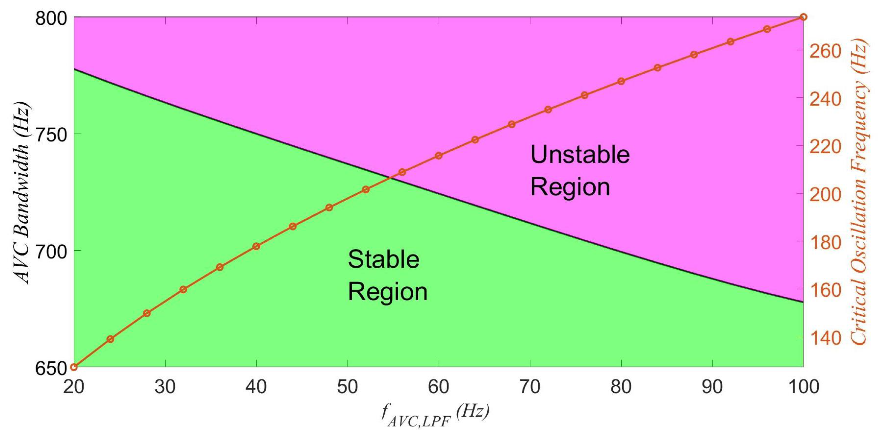
Similarly, the stability region of the AVC bandwidth in the strong grid case is shown in Figure 14. The critical AVC bandwidth is equal to approximately 781 Hz for $f_{\mathrm{AVC},\mathrm{LPF}}$ equal to 20 Hz; then it drops to approximately 673 Hz when the cutoff frequency varies from 24 to 100 Hz. The oscillation frequency that corresponds to the critical AVC bandwidth is equal to 127 Hz for $f_{\mathrm{AVC},\mathrm{LPF}}$ equal to 20 Hz. When $f_{\mathrm{AVC},\mathrm{LPF}}$ varies from 20 to 100 Hz, the oscillation frequency increases to 273 Hz.

5. Simulation Results

To verify the small-signal model dynamic response of the model, time domain simulations were carried out by using MATLAB Simulink and the PLECS block set. All of the simulation cases were implemented in weak and strong case scenarios. They were tested under three different cases of AVC’s low-pass filter, where $f_{\mathrm{AVC},\mathrm{LPF}}$ was equal to 20, 50, and 100 Hz. Fast Fourier transformation (FFT) was utilized in order to identify the dominant frequency when the system became unstable. Then, the comparison with the results in Section 3 could be done. The circuit and control parameters are shown in Appendix A.

5.1. Time Domain Analysis in Weak Grid Case Scenario

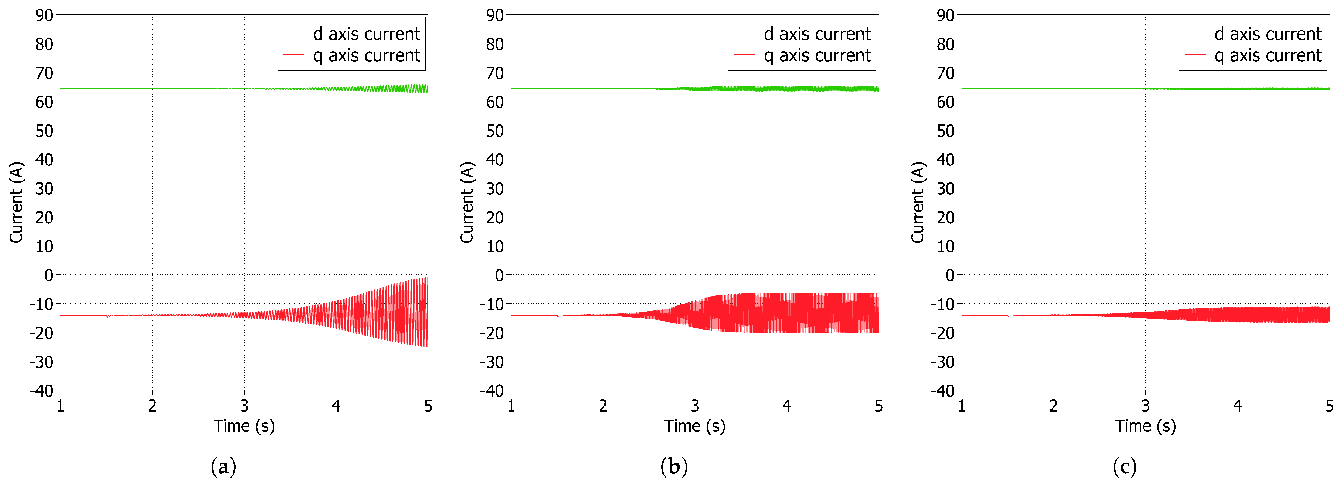
In the weak grid case scenario ($SCR=1.5$), the impact of PLL on the system’s stability was first tested under different cases of $f_{AVC,LPF}$. A step change was applied to the default proportional gain of the PLL $K_{P,PLL0}$ at $t=1.5$ seconds, when the system was stable. The controller’s gain then obtained the value that critically impacted the system’s stability ($K_{P,PLLcr}$), and the inductor current $I_L$ in the dq frame was utilized to demonstrate the instability cases. In Figure 15 and Figure 16, the $K_{P,PLLcr}$ and the corresponding critical frequency obtained from the FFT analysis are shown.

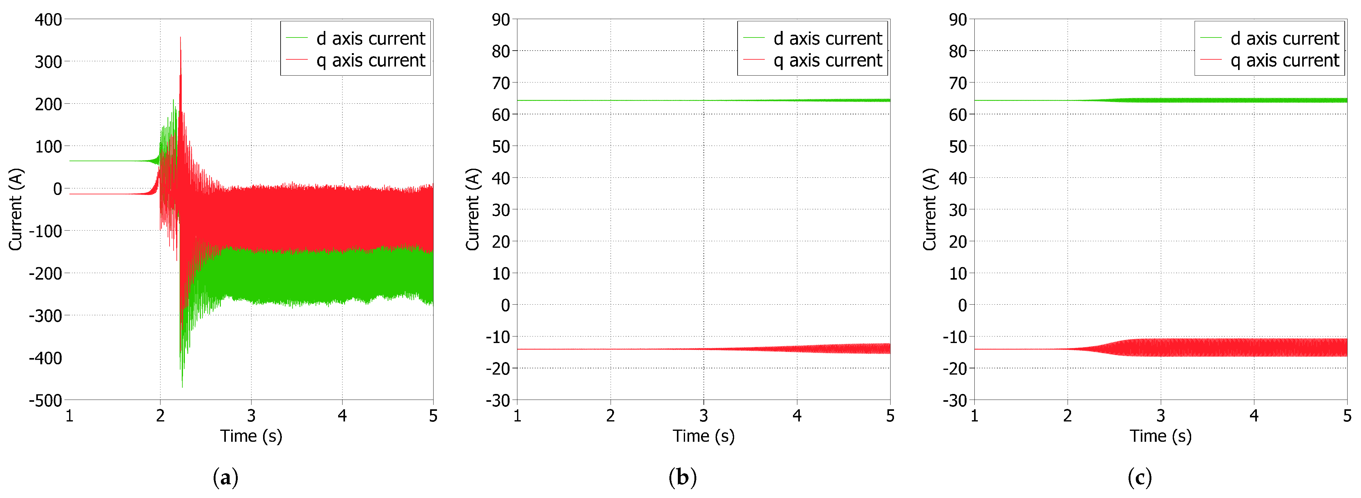
Then, the impact of the AVC bandwidth on the system’s stability was tested for the same cases of $f_{\mathrm{AVC},\mathrm{LPF}}$. A ramp change with a small slope was applied to the integral gain of the AVC $K_{\mathrm{I},\mathrm{a}0}$ at $t=1.5$ seconds when the system was stable, and the controller’s value that affected the system’s stability ($K_{\mathrm{I},\mathrm{a}\mathrm{c}\mathrm{r}}$) was identified. The inductor current in the dq frame was again utilized to demonstrate the instability cases. In Figure 17 and Figure 18, the $K_{\mathrm{I},\mathrm{a}\mathrm{c}\mathrm{r}}$ and the corresponding critical frequency obtained from the FFT analysis are shown.

The results in Figure 15, Figure 16, Figure 17 and Figure 18 are very close to the corresponding small-signal stability analysis in Figure 7 and Figure 8. Therefore, the eigenvalue-based stability analysis was validated in the weak grid case scenario and provides a high level of accuracy.

5.2. Time Domain Analysis in Strong Grid Case Scenario

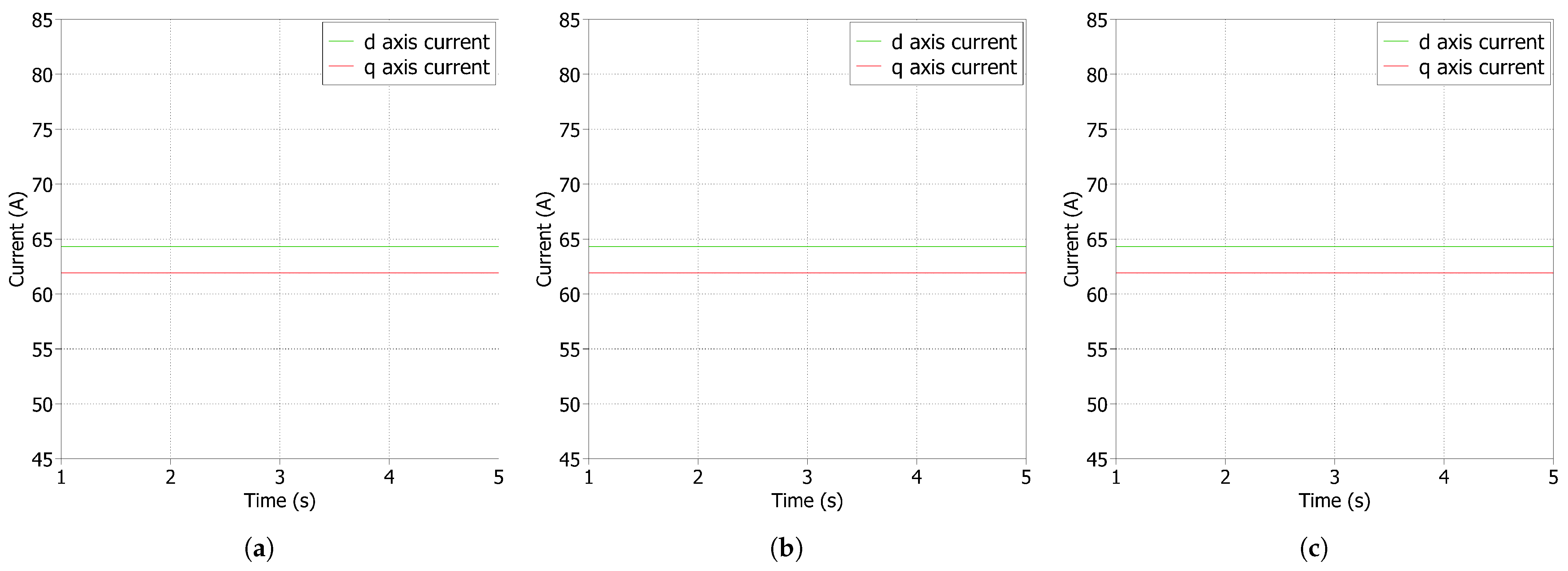
In the strong grid case scenario ($SCR=10$), the procedure was similar to the weak grid case scenario. First, the impact of PLL on the system’s stability was studied under different cases of $f_{\mathrm{AVC},\mathrm{LPF}}$. In all $f_{\mathrm{AVC},\mathrm{LPF}}$ cases, the same step change was applied to $K_{P,PLL0}$ at $t=1.5$ s (equal to 10 times $K_{P,PLL0}$) when the system was stable. The obtained time domain simulation results of the inductor current in the dq frame are shown in Figure 19 and prove that changes in $f_{\mathrm{AVC},\mathrm{LPF}}$ have no impact on the system’s stability even though $K_{P,PLL}$ is increased. Therefore, in the strong grid—and for all $f_{\mathrm{AVC},\mathrm{LPF}}$ cases—the system remains stable when the PLL bandwidth varies.

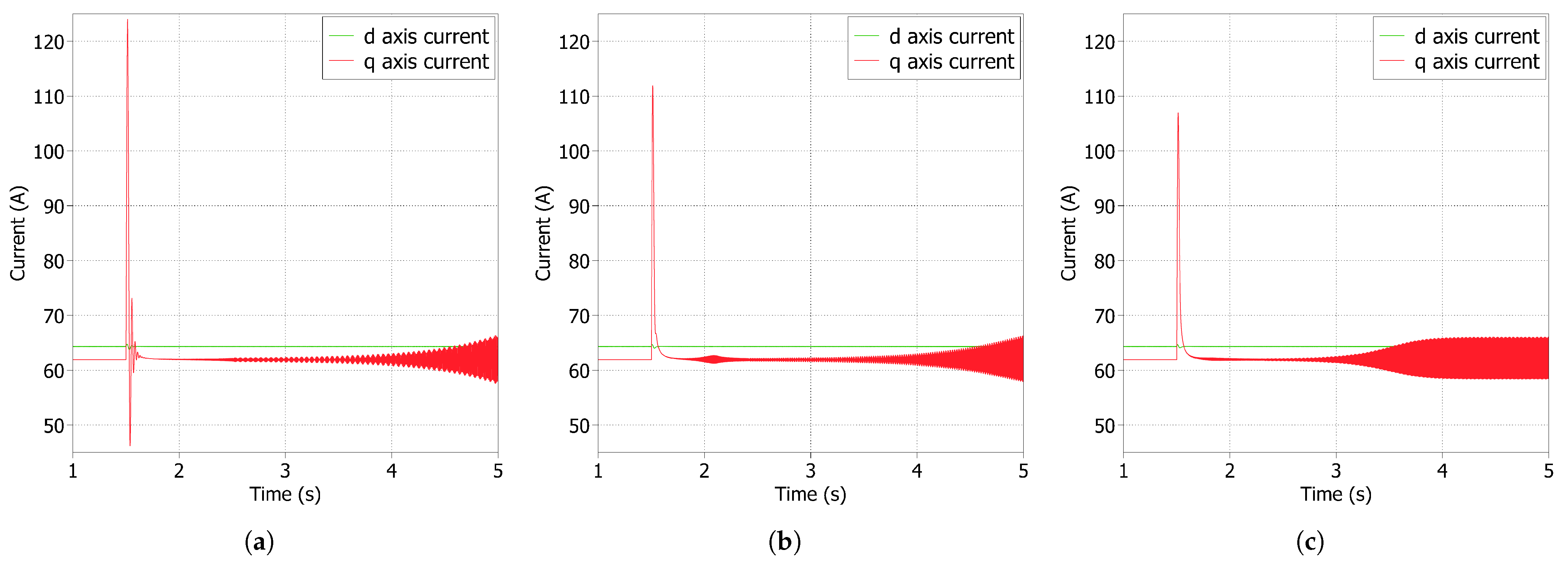
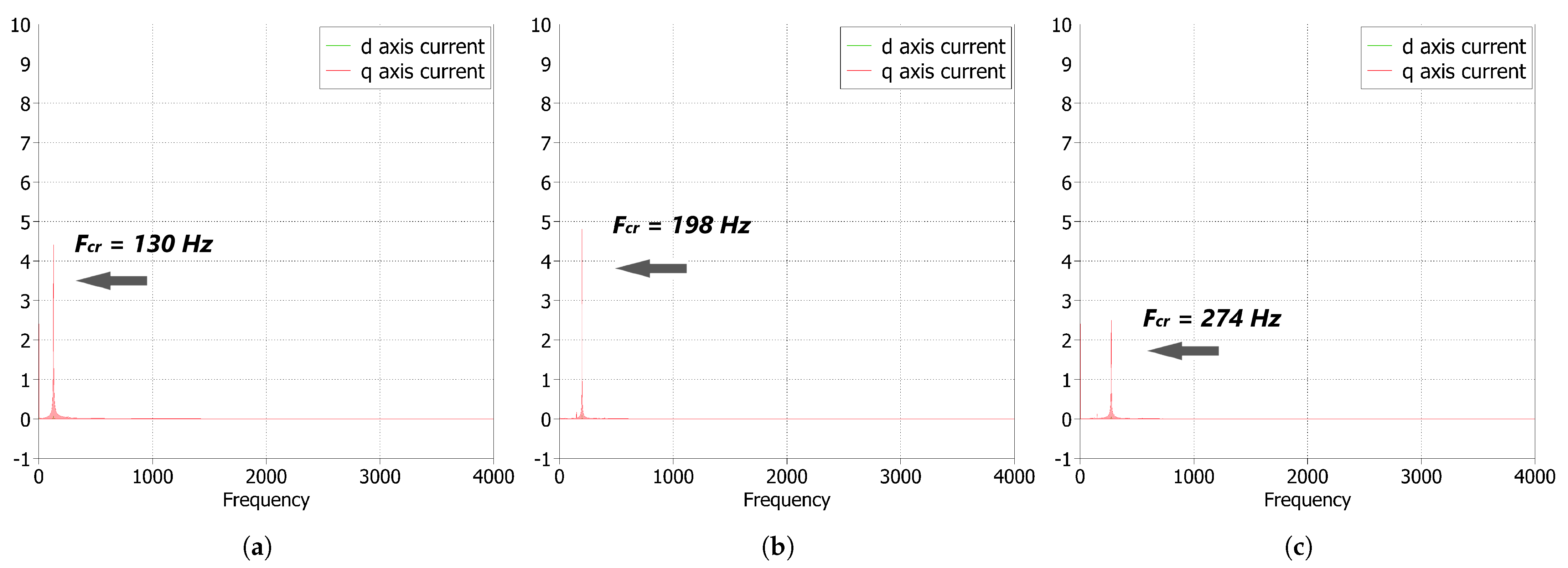
Similar to the weak grid case scenario, the impact of the AVC bandwidth on the system’s stability was observed during the simulation process for different $f_{\mathrm{AVC},\mathrm{LPF}}$ cases. A ramp change was applied to $K_{\mathrm{I},\mathrm{a}0}$ at t = 1.5 s when the system was stable; the slope was higher than in the weak grid case because the instability was observed in much higher AVC bandwidth. The graphs of the inductor current in the dq frame and the corresponding FFT analysis are presented in Figure 20 and Figure 21, which illustrate the instability cases.

The results in Figure 19, Figure 20 and Figure 21 are very close to the corresponding small-signal stability analysis in Figure 9 and Figure 10. Therefore, the eigenvalue-based stability analysis is accurately validated in the strong grid case scenario (just as in the weak grid case).

6. Conclusions

In this paper, the impact of the AVC in a grid-connected VSC of a wind turbine was studied under different grid strength cases that were defined by the SCR values of the system. The nonlinear state-space model of a grid-following VSC was built, where the converter was connected to the grid through an LC filter, and the individual state-space models of the PLL, the current controller, the AVC, and the digital time delay were developed in the dq reference frame. The eigenvalue-based stability analysis was used to assess the system’s stability, where the obtained eigenvalue traces showed the impact of each controller for different cases of $f_{\mathrm{AVC},\mathrm{LPF}}$. It is proven that the increase of $f_{\mathrm{AVC},\mathrm{LPF}}$ from 20 to 100 Hz decreases the critical AVC bandwidth in the strong and weak grid case scenarios—not very significant in the weak grid case—and increases the oscillation frequency that corresponds to the critical cases of instability. On the other hand, the increase of $f_{\mathrm{AVC},\mathrm{LPF}}$ decreases the critical PLL bandwidth in the weak grid case; however, the oscillation frequencies that correspond to the critical PLL bandwidth cases of instability follow an interesting trend, as they decrease for $f_{\mathrm{AVC},\mathrm{LPF}}=20$ to 50 Hz, and then increase until $f_{\mathrm{AVC},\mathrm{LPF}}$ reaches the value of 100 Hz. In the strong grid case, the PLL bandwidth does not impact the system’s stability even when $f_{\mathrm{AVC},\mathrm{LPF}}$ changes. Time domain simulations are provided, accompanied by the FFT analysis, demonstrating the validity of the outcomes in this research.

References

- GWEC: Global Wind Report 2022. Available online: https://gwec.net/globalwind-report-2022/ (accessed on 24 November 2022).
- Barnes, M.; Beddard, A. Voltage Source Converter HVDC Links—The State of the Art and Issues Going Forward. Energy Procedia 2012, 24, 108–122. [Google Scholar] [CrossRef]
- Rocabert, J.; Luna, A.; Blaabjerg, F.; Rodrguez, P. Control of Power Converters in AC Microgrids. IEEE Trans. Power Electron. 2012, 27, 4734–4749. [Google Scholar] [CrossRef]
- Ahmed, N.; Haider, A.; Van Hertem, D.; Zhang, L.; Nee, H.-P. Prospects and Challenges of future HVDC SuperGrids with Modular Multilevel Converters. In Proceedings of the 14th European Conference on Power Electronics and Applications, Birmingham, UK, 30 August–1 September 2011; pp. 1–10. [Google Scholar]
- Zou, C.; Rao, H.; Xu, S.; Li, Y.; Li, W.; Chen, J.; Zhao, X.; Yang, Y.; Lei, B. Analysis of Resonance Between a VSC-HVDC Converter and the AC Grid. IEEE Trans. Power Electron. 2018, 33, 10157–10168. [Google Scholar] [CrossRef]
- Li, C. Unstable Operation of Photovoltaic Inverter from Field Experiences. IEEE Trans. Power Deliv. 2017, 33, 1013–1015. [Google Scholar] [CrossRef]
- Buchhagen, C.; Rauscher, C.; Menze, A.; Jung, J. BorWin1—First Experiences with Harmonic Interactions in Converter Dominated Grids. In Proceedings of the International ETG Congress 2015; Die Energiewende—Blueprints for the New Energy Age, Bonn, Germany, 17–18 November 2015; pp. 27–33. [Google Scholar]
- Kocewiak, Ł.; Blasco-Gimenez, R.; Buchhagen, C.; Kwon, J.B.; Sun, Y.; Schwanka Trevisan, A.; Larsson, M.; Wang, X. Overview, Status and Outline of Stability Analysis in Converter-based Power Systems. In Proceedings of the 19th Wind Integration Workshop, Online, 11–12 November 2020; pp. 1–10. [Google Scholar]
- Wang, X.; Taul, M.G.; Wu, H.; Liao, Y.; Blaabjerg, F.; Harnefors, L. Grid-Synchronization Stability of Converter-Based Resources—An Overview. IEEE Open J. Ind. Appl. 2020, 1, 115–134. [Google Scholar] [CrossRef]
- Wang, X.; Harnefors, L.; Blaabjerg, F. A Unified Impedance Model of Grid-Connected Voltage-Source Converters. IEEE Trans. Power Electron. 2017, 33, 1775–1787. [Google Scholar] [CrossRef]
- Wang, X.; Loh, P.C.; Blaabjerg, F. Stability Analysis and Controller Synthesis for Single-Loop Voltage-Controlled VSIs. IEEE Trans. Power Electron. 2017, 32, 7394–7404. [Google Scholar] [CrossRef]
- Harnefors, L.; Bongiorno, M.; Lundberg, S. Input-Admittance Calculation and Shaping for Controlled Voltage-Source Converters. IEEE Trans. Ind. Electron. 2007, 54, 3323–3334. [Google Scholar] [CrossRef]
- Zhang, H.; Harnefors, L.; Wang, X.; Hasler, J.-P.; Ostlund, S.; Danielsson, C.; Gong, H. Loop-at-a-Time Stability Analysis for Grid-Connected Voltage-Source Converters. IEEE J. Emerg. Sel. Top. Power Electron. 2021, 9, 5807–5821. [Google Scholar] [CrossRef]
- Kroutikova, N.; Hernandez-Aramburo, C.A.; Green, T.C. State-Space Model of Grid-Connected Inverters under Current Control Mode. IET Electr. Power Appl. 2007, 1, 329–338. [Google Scholar] [CrossRef] [Green Version]
- Gontijo, G.F.; Bakhshizadeh, M.K.; Kocewiak, Ł.H.; Teodorescu, R. State Space Modeling of an Offshore Wind Power Plant With an MMC-HVDC Connection for an Eigenvalue-Based Stability Analysis. IEEE Access 2022, 10, 82844–82869. [Google Scholar] [CrossRef]
- Zhou, J.Z.; Ding, H.; Fan, S.; Zhang, Y.; Gole, A.M. Impact of Short-Circuit Ratio and Phase-Locked-Loop Parameters on the Small-Signal Behavior of a VSC-HVDC Converter. IEEE Trans. Power Deliv. 2014, 29, 2287–2296. [Google Scholar] [CrossRef]
- Amin, M.; Suul, J.A.; D’Arco, S.; Tedeschi, E.; Molinas, M. Impact of State-Space Modelling Fidelity on the Small-Signal Dynamics of VSC-HVDC Systems. In Proceedings of the 11th IET International Conference on AC and DC Power Transmission, Birmingham, UK, 10–12 February 2015; pp. 1–11. [Google Scholar]
- Rezaee, S.; Radwan, A.; Moallem, M.; Wang, J. Voltage Source Converters Connected to Very Weak Grids: Accurate Dynamic Modeling, Small-Signal Analysis, and Stability Improvement. IEEE Access 2020, 8, 201120–201133. [Google Scholar] [CrossRef]
- Musengimana, A.; Li, H.; Zheng, X.; Yu, Y. Small-Signal Model and Stability Control for Grid-Connected PV Inverter to a Weak Grid. Energies 2021, 14, 3907. [Google Scholar] [CrossRef]
- Gholami-Khesht, H.; Davari, P.; Novak, M.; Blaabjerg, F. A Probabilistic Framework for the Robust Stability and Performance Analysis of Grid-Tied Voltage Source Converters. Appl. Sci. 2022, 12, 7375. [Google Scholar] [CrossRef]
- Agbemuko, A.J.; Domínguez-García, J.L.; Gomis-Bellmunt, O.; Harnefors, L. Passivity-based Analysis and Performance Enhancement of a Vector Controlled VSC Connected to a Weak AC Grid. IEEE Trans. Power Deliv. 2020, 36, 156–167. [Google Scholar] [CrossRef]
- Dimitropoulos, D.; Wang, X.; Blaabjerg, F. Small-Signal Stability Analysis of Grid-Connected Converter under Different Grid Strength Cases. In Proceedings of the 2022 IEEE 13th International Symposium on Power Electronics for Distributed Generation Systems (PEDG), Kiel, Germany, 26–29 June 2022; pp. 1–6. [Google Scholar]
- Wen, B.; Boroyevich, D.; Burgos, R.; Mattavelli, P.; Shen, Z. Analysis of dq small-signal impedance of grid-tied inverters. IEEE Trans. Power Electron. 2015, 31, 675–687. [Google Scholar] [CrossRef]
- Rosso, R. Stability Analysis of Converter Control Strategies for Power Electronics-Dominated Power Systems. Ph.D. Thesis, Christian-Albrecht University of Kiel, Kiel, Germany, 2020. [Google Scholar]
Figure 1.
Grid-following VSC converter connected to the grid with its control structure.
Figure 2.
Control and grid dq frame used for the VSC.
Figure 3.
Control structure of the used PLL in Figure 1.
Figure 4.
Control structure of the current controller (PIcc) in Figure 1.
Figure 5.
Control structure of the alternate voltage controller (AVC) in Figure 1.
Figure 6.
LC filter and grid impedance circuit in Figure 1.
Figure 7.
Eigenvalue−based stability analysis for different AVC filter cases in the weak grid case scenario (SCR = 1.5). The critical bandwidth of the PLL is identified after varies from 0.1 (deep blue) to 10 (deep red) times. (a) Hz (b) Hz (c) Hz.
Figure 8.
Eigenvalue−based stability analysis for different AVC filter cases in the weak grid case scenario (SCR = 1.5). The critical bandwidth of the AVC is identified after varies from 0.1 (deep blue) to 10 (deep red) times. (a) Hz (b) Hz (c) Hz.
Figure 9.
Eigenvalue−based stability analysis for different AVC filter cases in the strong grid case scenario (SCR = 10). varies from 0.1 (deep blue) to 10 (deep red) times. (a) Hz (b) Hz (c) Hz.
Figure 10.
Eigenvalue−based stability analysis for different AVC filter cases in the strong grid case scenario (SCR = 10). The critical bandwidth of the AVC is identified after varies from 1 (deep blue) to 200 (deep red) times. (a) Hz (b) Hz (c) Hz.
Figure 11.
Stability regions of PLL bandwidth in weak grid case (SCR = 1.5), when varies from 20 to 100 Hz. The corresponding critical oscillation frequency to the critical PLL bandwidth is shown (red).
Figure 12.
Stability regions of AVC bandwidth in weak grid case (SCR = 1.5), when varies from 20 to 100 Hz. The corresponding critical oscillation frequency to the critical AVC bandwidth is shown (red).
Figure 13.
Stability regions of PLL bandwidth in strong grid case (SCR = 10), when varies from 20 to 100 Hz. The system is stable for the PLL bandwidth in question; therefore, no critical oscillation frequencies are shown.
Figure 14.
Stability regions of the AVC bandwidth in a strong grid case (SCR = 10), when varies from 20 to 100 Hz. The corresponding critical oscillation frequency to the critical AVC bandwidth is shown (red).
Figure 15.
Time domain simulations of the VSC inductor current for different AVC filter cases. The stability impact of PLL in a weak grid (SCR = 1.5) was observed, caused after the step change in to its critical value at t=1.5 s; (a) when Hz; (b) when Hz; (c) when Hz.
Figure 16.
FFT analysis of the VSC inductor current for different AVC filter cases in a weak grid (SCR = 1.5). The dominant oscillation frequency is shown when obtains its critical value; (a) Hz; (b) Hz; (c) Hz.
Figure 17.
Time domain simulations of the VSC inductor current for different AVC filter cases. The stability impact of AVC in the weak grid (SCR = 1.5) is observed, caused after the ramp change in to its critical value at t = 1.5 s; (a) when Hz; (b) when Hz; (c) when Hz.
Figure 18.
FFT analysis of the VSC inductor current for different AVC filter cases in the weak grid (SCR = 1.5). The dominant oscillation frequency is shown when obtains its critical value; (a) Hz (b) Hz (c) Hz.
Figure 19.
Time domain simulations of the VSC inductor current for different AVC filter cases. The step change in PLL’s proportional gain at t = 1.5 s from to has no stability impact in the strong grid case (SCR = 10); (a) Hz;(b) Hz; (c) Hz.
Figure 20.
Time domain simulations of the VSC inductor current for different AVC filter cases. The stability impact of AVC in a strong grid (SCR = 10) is observed, caused after the ramp change in to its critical value at t = 1.5 s; (a) when Hz; (b) when Hz; (c) when Hz.
Figure 21.
FFT analysis of the VSC inductor current for different AVC filter cases in the strong grid (SCR = 10). The dominant oscillation frequency is shown when obtains its critical value; (a) Hz; (b) Hz; (c) Hz.
Disclaimer/Publisher’s Note: The statements, opinions and data contained in all publications are solely those of the individual author(s) and contributor(s) and not of MDPI and/or the editor(s). MDPI and/or the editor(s) disclaim responsibility for any injury to people or property resulting from any ideas, methods, instructions or products referred to in the content. |
© 2023 by the authors. Licensee MDPI, Basel, Switzerland. This article is an open access article distributed under the terms and conditions of the Creative Commons Attribution (CC BY) license (https://creativecommons.org/licenses/by/4.0/).
Share and Cite
MDPI and ACS Style
Dimitropoulos, D.; Wang, X.; Blaabjerg, F. Stability Impacts of an Alternate Voltage Controller (AVC) on Wind Turbines with Different Grid Strengths. Energies 2023, 16, 1440. https://doi.org/10.3390/en16031440
AMA Style
Dimitropoulos D, Wang X, Blaabjerg F. Stability Impacts of an Alternate Voltage Controller (AVC) on Wind Turbines with Different Grid Strengths. Energies. 2023; 16(3):1440. https://doi.org/10.3390/en16031440
Chicago/Turabian StyleDimitropoulos, Dimitrios, Xiongfei Wang, and Frede Blaabjerg. 2023. "Stability Impacts of an Alternate Voltage Controller (AVC) on Wind Turbines with Different Grid Strengths" Energies 16, no. 3: 1440. https://doi.org/10.3390/en16031440
Note that from the first issue of 2016, this journal uses article numbers instead of page numbers. See further details here.