Aggregating Prophet and Seasonal Trend Decomposition for Time Series Forecasting of Italian Electricity Spot Prices

Abstract

The cost of electricity and gas has a direct influence on the everyday routines of people who rely on these resources to keep their businesses running. However, the value of electricity is strongly related to spot market prices, and the arrival of winter and increased energy use owing to the demand for heating can lead to an increase in energy prices. Approaches to forecasting energy costs have been used in recent years; however, existing models are not yet robust enough due to competition, seasonal changes, and other variables. More effective modeling and forecasting approaches are required to assist investors in planning their bidding strategies and regulators in ensuring the security and stability of energy markets. In the literature, there is considerable interest in building better pricing modeling and forecasting frameworks to meet these difficulties. In this context, this work proposes combining seasonal and trend decomposition utilizing LOESS (locally estimated scatterplot smoothing) and Facebook Prophet methodologies to perform a more accurate and resilient time series analysis of Italian electricity spot prices. This can assist in enhancing projections and better understanding the variables driving the data, while also including additional information such as holidays and special events. The combination of approaches improves forecast accuracy while lowering the mean absolute percentage error (MAPE) performance metric by 18% compared to the baseline model.

1. Introduction

The price of electricity and gas directly affects the routine of the people who need this availability to maintain their daily activities. With the Russia–Ukraine conflict that started on 24 February 2022, the value of electricity and gas has increased considerably for consumers in neighboring countries. The value of electricity is directly linked to the value of spot market prices [1], and with the onset of winter and increased energy consumption due to the need for heating, the value that energy can reach is something that needs to be assessed [2].

Several authors have been researching this subject in recent years. Various approaches based on artificial intelligence paradigms—mainly machine learning and deep learning—have been designed to forecast the price of energy [3,4,5]. Before the deregulation of electricity markets, spot price forecasts were laborious and detailed [6]. They were based on estimating the future market forecast based on historical data, calculating supply by adding the operating costs of generating units, and by comparing supply and demand. Thus, cost-based models were reliable tools for forecasting electricity spot prices and required negligible changes. However, currently, such models are outdated, and unfortunately, the models implemented at present for electricity spot prices are not yet accurate enough [3].

Due to increasing competition, seasonal variations on the demand and supply sides, seasonal variations in temperature, the availability of renewable energy sources in the energy systems, macroeconomics, and many other factors, it is essential to develop more accurate price modeling and new forecasting techniques, which is a challenge for market participants [7]. As electricity cannot be stored, a balance must be maintained between demand and supply, thus electricity spot markets can have opportunities and risks. Thus, it is important to develop profitable strategies using appropriate tools that require accurate day-ahead electricity spot prices, where large amounts of electricity are commercialized daily. The daily price volatility is high, they are also characterized by high frequency, a variable average, and multiple seasonality due to several unique characteristics that differentiate electricity from other forms of energy [8].

The European wholesale electricity price data refers to the prices of electricity that are traded on the wholesale market in Europe [9]. Wholesale electricity markets are where electric utilities, large industrial users, and other electricity generators buy and sell electricity in bulk. These markets are typically organized and regulated by national or regional regulatory bodies. As mentioned by Bahn, Samano, and Sarkis [10], the use of renewable energy has changed electricity market prices; according to the authors, the merit order effect has a downward pressure on prices whereas, with market power, higher infra-marginal rents will tend to increase prices.

The formation of wholesale electricity prices in Europe is influenced by a variety of factors, including the supply and demand for electricity, the cost of generation and transmission, and the availability of different types of electricity generation [11]. On the supply side, the availability of electricity is influenced by factors such as the capacity of electricity generation facilities, the availability of fuel sources, and the reliability of transmission and distribution systems [12]. On the demand side, the demand for electricity is influenced by factors such as economic activity, population growth, and changes in consumer behavior.

The cost of electricity generation and transmission is also an important factor in the formation of wholesale electricity prices [13]. This includes the cost of fuel sources, such as coal, natural gas, and renewable energy sources, as well as the cost of maintaining and operating electricity generation and transmission infrastructure [14]. The availability of different types of electricity generation can also affect the formation of wholesale electricity prices. For example, the use of renewable energy sources, such as wind and solar power, can help to reduce the overall cost of electricity generation, which may lead to lower wholesale electricity prices [15].

In the literature, there are many recent works related to energy consumption in Italy. Some researchers have especially studied this variation due to the pandemic, such as the works of Ghiani et al. [16], Bahmanyar, Estebsari, and Ernst [17], and Krarti, and Aldubyan [18]. Current studies related to the price of energy, such as the work of Moreno and Díaz [19], are rarer, and the analyses performed are in relation to previous years [20] in which there was not such a wide variation in the time series; this is the challenge of this research. One of the latest works related to electricity prices in Italy is presented by Ghanem et al. [21], wherein an evaluation is also performed due to the impact of the coronavirus disease of 2019 (COVID-19).

Different time frames, such as short-term, medium-term, and long-term, can be used for forecasting [22]. When developing a forecast, the time horizon of the forecast might impact which aspects are most important to examine. Short-term forecasting may place a greater emphasis on current market conditions and immediate supply and demand dynamics. Seasonal changes and the adoption of new technology may be more meaningful for medium-term forecasting. For long-term forecasting, it may be crucial to include macroeconomic trends and structural changes in the market. It is essential to evaluate the time horizon of the forecast and the elements that are likely to influence the forecast for that horizon [23].

The development of more accurate forecasting methodologies has become more complex and dynamic, and is a key task for investors when planning their bidding strategies to maximize their effectiveness from short, medium, and long-term horizons [24,25,26]. Finally, they help regulators ensure the long-term sufficiency and security of supply and the constancy of energy markets. For these reasons, there has been growing interest in the literature with respect to developing better price modeling and forecasting techniques [27,28,29]. Based on that, an assessment will be presented of the variation in electricity prices on the stock market in Italy, which is reflected in the increase in the cost of energy for consumers.

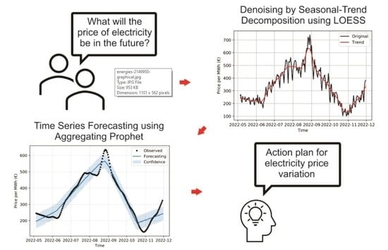
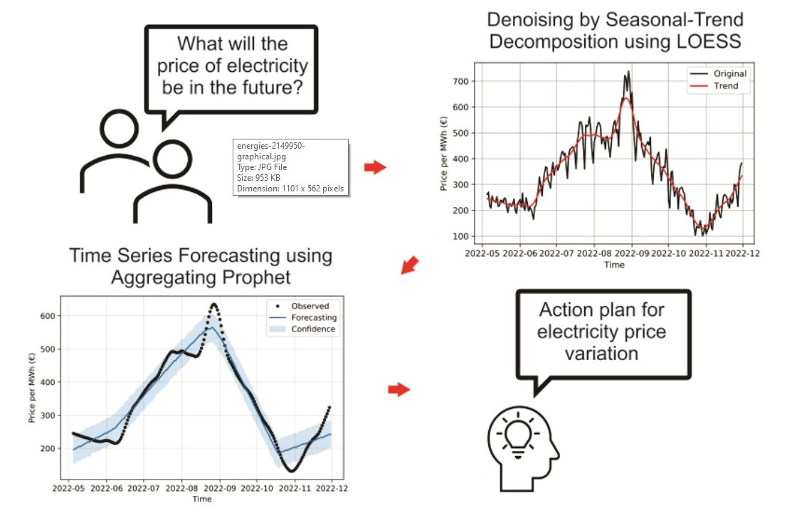
Summarily, the contributions of this paper are:

• Developing a less error-prone forecasting model for electricity spot prices, which combines Facebook’s Prophet approach and the seasonal and trend decomposition using LOESS (locally estimated scatterplot smoothing);
• Performing a pre-processing filter to reduce noise in the time series, avoiding the evaluation of abrupt variations that do not correspond to a variation trend;
• Evaluating stock market behavior in relation to days of the week, time of year, and variation trend, based on the mean square error, root-mean-square error, and mean absolute percentage error.

The rest of this article is structured in the following way. Section 2 reviews the related works in the forecasting theme applied to electricity prices and related fields. Then, this Section describes the dataset and preprocessing steps of electricity prices in Italy. Facebook’s Prophet method and Seasonal and Trend decomposition using LOESS (STL) are introduced in Section 3. Section 4 summarizes and discusses the forecasting results. Finally, concluding remarks and potential future directions are given in Section 5.

2. Related Works

In the European Union (EU), the wholesale electricity price is decided by the last power plant needed to meet demand [9]. Wind, nuclear, coal, and gas power facilities submit bids to the electricity market, with the lowest sources chosen first. In this approach, gas plants often set prices. This approach ensures that all generators sell their power at the same price, allowing cheaper renewable energy generators to have a wider profit margin as an incentive for increasing investment in renewable energy, which the EU needs in order to accomplish its climate change goals [11].

The uncertain future value of electricity has drawn the attention of several authors who have proposed solutions to reduce the impact of price variation, by preparing the market for possible price hikes and the need for rationing [30]. To solve this issue, researchers have been conducting evaluations on the possibility of optimizing the power generation scheduling [31], optimization in equipment design [32], and improvements in the identification of faults in the electrical power system based on computer vision techniques [33], standard classifiers [34], classical convolutional neural networks [35], and using interpretable models [36]. A further possibility that has been explored is the estimation of the future value of electricity based on time series forecasting [37], which is the focus of this paper.

Defining which model is appropriate for the evaluation of electricity spot prices can be a challenging task since there are large fluctuations in the energy market due to external factors [38], as well as uncertainties regarding wind power generation [39]. Ensemble-based models that use weak learners to have a robust model are increasingly being used. More recently, the decomposition ensemble forecasting paradigm has been proposed for energy price forecasting. This approach often decomposes time series data into several components with simple structures and aggregates the forecast results from all the components to obtain a final forecast [40]. Models that are increasingly being applied for time series forecasting include the group method of data handling [41], ensemble learning models [42], long short-term memory [43], and other classical approaches [44].

Three electricity price series from Australian and Spanish electricity markets were used to verify the prediction performance of a hybrid model, with a two-layer decomposition based on the combination of variational modal decomposition (VMD) and ensemble empirical modal decomposition (EEMD) carried out on the residual term, combining the extreme learning machine (ELM) optimized by differential evolution (DE). The generalization ability and effectiveness of the proposed model were verified through tests on data with different characteristics [40]. The proposed decomposition–ensemble learning models, using randomized algorithms as individual forecasting tools, were extremely efficient and fast compared with other benchmarking models for energy forecasting the Brent crude oil spot price and the Henry Hub natural gas price [45].

The bagging, boosting, random subspace, bagging plus random subspace, and stacked generalization ensemble models were applied to predict emergency situations 1-h ahead in hydroelectric power plants, with the dam, installed at Santa Catarina state, Brazil, advancing the necessary decision-making in a situation of risk to the dam [46]. A very short-term electricity price forecasting model was developed by Bhatia et al. [47], applying ensemble learning. The model combined bagging and boosting in the stacking phase, reducing the overall variances due to the stacking process by inculcating bootstrap aggregation. Improved forecasting performance in terms of accuracy and statistical tests was obtained. Were utilized data for day-ahead electricity price, load consumption, wind generation, and other parameters, in Austria from January 2015 to December 2016.

The research of Jiang et al. [48] proposed a new decomposition–selection–ensemble forecasting system adopting multiple predictors to forecast time series, which can lift the restriction of a single model, and can objectively and adaptively select the best predictor for every sub-series via an optimal sub-model selection scheme, determining the most appropriate sub-models without being subjective. They selected two datasets of crude oil and natural gas future prices. The proposed model always achieves high-quality precision and stability relative to other models.

Ribeiro et al. [49] proposed a self-adaptive, decomposed, heterogeneous, and ensemble learning model for short-term electricity price forecasting. The coyote optimization algorithm was adopted to tune the decomposition hyperparameters in an empirical complementary ensemble manner in the preprocessing stage, and three machine learning models were designed with the intention of handling the components obtained through the signal decomposition approach with a focus on time series forecasting. The results showed the efficiency of the proposed model. A predictive model was developed by Lucas et al. [50] to capture the dynamics and identify deterministic or quasi-determinist variables which may influence the energy market prices. A total of 19 predictors were considered to develop a regression model using three machine learning algorithms. In terms of feature importance, many variables were analyzed and scores were assigned, and the ELEXON Balancing Energy Market in the United Kingdom was considered. The proposed approach could be used as a support tool for market price forecasting.

Hybrid models that use noise reduction techniques increase the model’s ability to perform accurate predictions [51]. A novel hybrid prediction model was proposed in the work of Qiao and Yang [52] using the wavelet transform (WT), stacked autoencoders, and long short-term memory. Compared with other advanced prediction models, the forecasting accuracy of the developed model is obviously improved based on some general evaluation indexes. In addition, this model overcomes the shortcomings of determining wavelet’s orders and layers based on experience. Its prediction accuracy is higher than that of using long short-term memory alone to predict residential, commercial, and industrial electricity prices [53].

Techniques combining WT with fixed and adaptive machine learning time series models have been evaluated [53]. To create an adaptive model, an extended Kalman filter was used to update the parameters continuously on the test set. This paper compared two approaches combining WT with prediction models—multicomponent and direct—applied to stationary and non-stationary data from the United Kingdom electricity demand/gas price markets. The results showed that the forecasting accuracy is significantly improved by using the WT and adaptive models. Another study using a novel hybrid method with empirical wavelet transform (EWT), support vector regression, bi-directional long short-term memory, and Bayesian optimization, was proposed to increase the accuracy of electricity price forecasting [54]. The proposed hybrid model is employed on the data gathered from the European Power Exchange Spot. Five different case studies were adopted to verify the effectiveness of the hybrid model that achieved a better forecasting performance. The use of WT is a promising alternative because it considers the signal energy to be superior to other filters [55].

In addition to noise reduction, optimizers have been applied to improve the predictive power of the model [56]. Thus, a new adaptive hybrid model based on variational mode decomposition, self-adaptive particle swarm optimization, seasonal autoregressive integrated moving average, and a deep belief network was proposed for short-term electricity price forecasting [57]. The effectiveness of the model was verified by using data from Australian, Pennsylvania–New Jersey–Maryland, and Spanish electricity markets. Results showed that the proposed model can significantly improve forecasting accuracy and stability.

Accurate forecasting of electricity spot prices is important for market participants [58], investors, and regulators [59]. A number of different methods have been proposed for this task, including time series models [60], artificial neural networks [61], and hybrid models. Ensemble-based models and decomposition ensemble forecasting have been found to be effective in forecasting electricity spot prices, as have hybrid models combining time series models with artificial neural networks. Self-adaptive, decomposed, heterogeneous and ensemble learning models have also been shown to be effective in this context. From the literature review, it is possible to observe that hybrid models and ensemble-based approaches are particularly effective for forecasting electricity spot prices, particularly in the short and medium term.

In summary, there has been a focus on finding efficient and effective methods for forecasting electricity prices in order to reduce the impact of price variation and prepare the market for potential price hikes and the need for rationing [30,37]. It is inferred from the literature review that hybrid models and ensemble-based approaches are particularly effective for forecasting electricity spot prices, particularly in the short and medium term.

This work is distinct from other research in a number of respects. The first objective is to create a less error-prone power spot price forecasting model by combining the Facebook Prophet technique with seasonal and trend decomposition using LOESS. Second, it incorporates a pre-processing filter to decrease noise in the time series and prevent the evaluation of abrupt variations that do not match a trend variation. The report concludes by evaluating the behavior of the stock market in connection to weekdays, seasons, and variance trends.

Dataset

In this paper, we utilized the European wholesale electricity price dataset to investigate the factors that influence the formation of wholesale electricity prices in Europe. This dataset includes time series data on the prices of electricity that are traded on the wholesale market in Europe, as well as information on the supply and demand for electricity, the cost of generation and transmission, and the availability of different types of electricity generation. For time series evaluation, the stock values of the electricity market of Italy from 1 January 2015 to 30 November 2022 were used, corresponding to 2890 observations (https://ember-climate.org/data-catalogue/european-wholesale-electricity-price-data/ (accessed on 23 December 2022)), corresponding to a daily record of the price variation, where the values are presented in megawatt-hour (MWh).

Using statistical and machine learning techniques, we analyzed the European wholesale electricity price dataset to understand trends and patterns in the data and to make predictions about future electricity prices [62]. Our analysis aims to identify the key factors that contribute to the formation of wholesale electricity prices in Europe and to provide insights into the factors that may impact the future direction of the electricity market.

3. Facebook’s Prophet Method

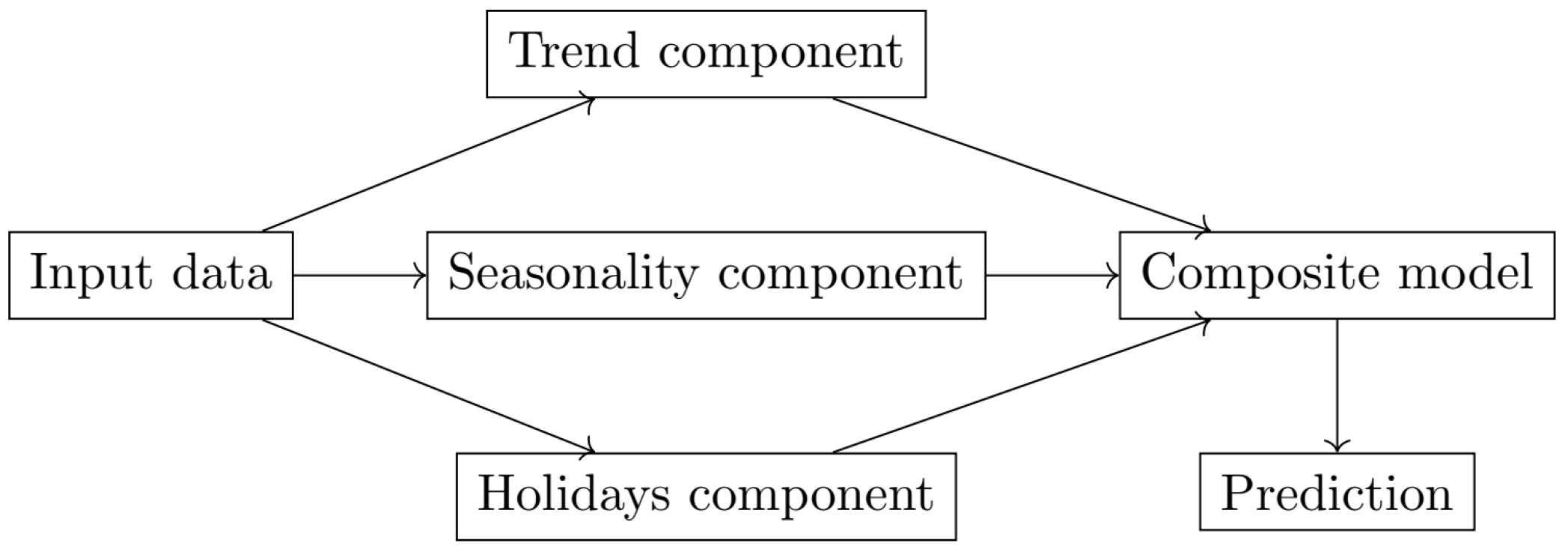
Facebook Prophet is a time series data forecasting tool created by Facebook’s Core Data Science team. It is constructed on top of the open-source programming language R and is intended to be simple to use while producing credible forecasts, according to [63]. The Prophet technique is based on the assumption that time series data can be described as a mixture of numerous characteristics, such as trends, seasonality, and holidays [64]. The math powering Facebook Prophet entails identifying and modeling these components using a number of mathematical and statistical methodologies: (i) linear regression is used to model the trend component of a time series; (ii) Fourier series are used to model the seasonality component of a time series; and (iii) additive models are used to describe the holidays component of a time series.

A linear or nonlinear regression model is often used to discover and model any underlying patterns or trends in the data for the trend component of the time series. A linear regression model’s equation can be given by:

$$y={\beta }_0+{\beta }_{1}x+ϵ,$$

where y is the dependent variable (i.e., the time series), x is the independent variable (i.e., the time of the data point), ${\beta }_0$ and ${\beta }_1$ are the coefficients of the model that are determined by the regression, and $ϵ$ is the error term representing the difference between the predicted value of y and the actual value.

A Fourier series, a mathematical tool for describing periodic functions, is generally used to model the seasonality component of a time series. A Fourier series can be represented as the sum of sines and cosines:

$$f\left(t\right)=a_0+\sum _{k=1}^n\left(a_{k}cos\frac{2\pi kt}{T}+b_{k}sin\frac{2\pi kt}{T}\right),$$

where $f\left(t\right)$ is the time series, t is the time of the data point, T is the period of the time series, n is the number of terms in the series, $a_0$ is the average value of the time series, $a_k$ and $b_k$ are the coefficients of the sines and cosines that are determined by the Fourier analysis.

The holidays component of the time series is often modeled using a generative additive model (GAM), a statistical model that allows for the insertion of additional elements that may influence the time series. According to [65], a GAM is a flexible and non-parametric regression model that may be used to match complex data patterns. This is accomplished by representing the relationship between the response variable (the time series data) and the predictor variables (the factors influencing the data) as a sum of smooth functions. The GAM used by the Prophet method can be expressed as follows:

$$y\left(t\right)=g_1\left(t\right)+g_2\left(t\right)+\cdots +g_k\left(t\right)+ϵ\left(t\right),$$

(1)

where $y\left(t\right)$ is the response variable (the time series data), $g_i\left(t\right)$ is the smooth function that models the $i\mathrm{th}$ predictor variable, and $ϵ\left(t\right)$ is the error term that represents the random noise or variation in the data.

Smooth functions $g_i\left(t\right)$ can be described using a number of basis functions that can capture the data’s complexity, such as splines or Fourier series. Maximum likelihood estimation or other optimization approaches can be used to estimate the parameters of these basis functions.

Once the GAM has been fitted to the data, it may be used to predict future values of t by evaluating the smooth functions $g_i\left(t\right)$. This will generate a forecast of the time series data, as well as uncertainty intervals that can be used to assess the forecast’s trustworthiness. After modeling these components, they can be integrated to generate a single, composite model of the time series (as is presented in Figure 1). Based on the detected and modeled underlying trends, patterns, and factors, this model can then be used to forecast future values of the time series.

The math behind the Facebook Prophet approach is based on the usage of generalized additive models, which are flexible and non-parametric regression models that may be utilized to model complex data patterns. The Prophet technique can generate trustworthy projections of time series data by utilizing these models. The method, in addition to forecasting, offers several other properties that can be beneficial for evaluating time series data. It may, for example, detect and model the impacts of holidays and other special events on data, and it can give visualizations of the data and the fitted model to aid comprehension.

3.1. Seasonal and Trend Decomposition Using LOESS (STL)

STL is a method for decomposing a time series into its trend, seasonality, and residual components. It entails applying a smoothing function to the data and then iteratively deleting the fitted curve from the data to extract the trend and seasonality components. The residuals, or the difference between the original data and the fitted curve, show noise or irregularity in the data [66].

Smoothing functions that can be employed in the STL approach include the LOESS and Savitzky-Golay (SG) filters. LOESS is a non-parametric smoothing approach that fits a smooth curve to the data using local regression. It is good at smoothing noisy data and is more adaptable than other smoothing approaches. The SG filter is a sort of digital smoothing filter that fits a polynomial function to a window of data points and uses the polynomial value at the window’s center point as the smoothed value. It is effective in removing noise while maintaining the underlying trend and structure of the data, according to [67].

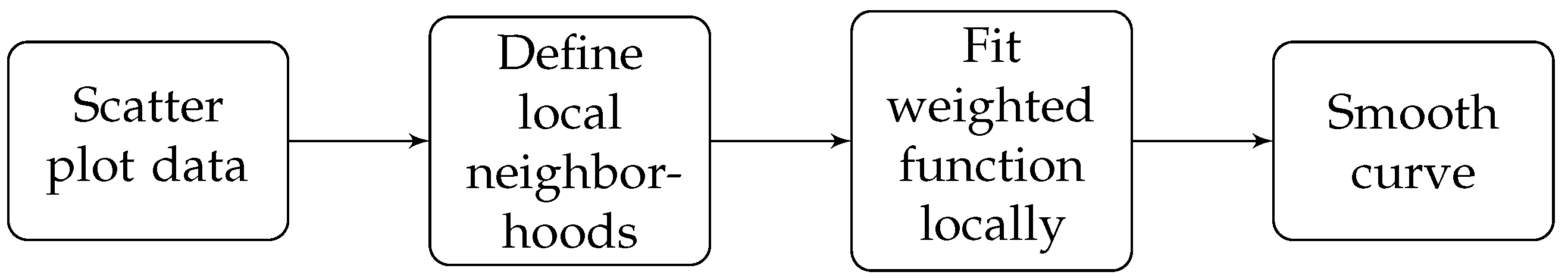
This study focused on STL utilizing LOESS, by fitting a smooth curve to each subset of the data separately and then merging these curves to obtain a global fit. This enables the LOESS approach to capture complicated patterns in data that would be difficult to express using a basic mathematical model. To utilize the LOESS method to fit a smooth curve to these data, we must first define the number of subsets to be employed. Typically, this is determined by the quantity of data points and the desired smoothness of the curve. If we have 100 data points and want a somewhat smooth curve, we may utilize 10 subsets. The data are separated into the required number of subgroups when the number of subsets is specified. If we utilize ten subsets, for example, we would divide the data into ten groups of ten data points each.

In the context of STL decomposition, the LOESS method is used in STL decomposition to fit separate smooth curves to the seasonal, trend, and residual components of time series data. These curves are then integrated to form a global fit to the data, which can be used to construct forecasts. To execute STL decomposition, the period of the seasonal component must first be specified, which is often the number of time units (such as months or years) in a single cycle of the seasonal pattern. Once the seasonal component’s period has been set, the STL technique proceeds as follows:

• The time series data are separated into seasons, each with a set number of time units. For example, if the data includes monthly retail sales with a seasonal span of 12 months (1 year), each season would have 12 months of data;
• Each season’s data are fitted with an LOESS smooth curve independently. This generates a sequence of smooth curves, one for each data season;
• Step 2—smooth curves are then joined to give a global fit to the data. The seasonal component of the time series is represented by this global fit;
• To create a detrended series, the seasonal component is eliminated from the original time series data. This detrended series only includes the data’s trend and residual components;
• The detrended series is then fitted with an LOESS smooth curve. This smooth curve represents the time series’ trend component;
• The residual component is then calculated by subtracting the trend component from the detrended series. These are the data that cannot be explained by seasonal or trend components.

Once the seasonal, trend, and residual components of the time series data have been extracted, they can be studied separately to acquire a better understanding of the data’s underlying patterns and trends. The trend component, for example, can indicate key patterns that repeat at regular intervals, whereas the seasonal component can disclose important patterns that repeat at regular intervals.

The residual component, on the other hand, can provide information about random noise or volatility in the data that the seasonal or trend components cannot explain. This can be helpful in determining the dependability of seasonal and trend estimations, as well as finding potential outliers or abnormalities in the data.

The STL approach can be used to forecast time series data after the components have been removed and examined. This is accomplished by extrapolating the smooth curves fitted to the data in steps 2 and 5. The seasonal and trend curves are projected to future time points and then put together to give a time series data forecast. The equation for STL decomposition is as follows:

$$y_t=S_t+T_t+R_t,$$

(2)

where $y_t$ is the original time series data, $S_t$ is the seasonal component, $T_t$ is the trend component, and $R_t$ is the residual component.

Seasonal decomposition with LOESS is accomplished mathematically by fitting a smooth curve to the data using locally weighted regression. This is often accomplished using a weighted least squares method, with the weights determined based on the data’s local features. The equation for locally weighted regression is as follows:

$$y=f\left(x\right)+ϵ,$$

where y is the dependent variable (i.e., the time series), $f\left(x\right)$ is the locally weighted regression curve, and $ϵ$ is the error term representing the difference between the predicted value of y and the actual value.

The locally weighted regression curve can be estimated by:

$$\begin{array}{c}\hfill min\sum _{i\in \mathcal{X}}{w}_i{(y_i-{\theta }^T{x}_i)}^2,\end{array}$$

(3)

where x is the independent variable (i.e., the time of the data point), w is a non-negative weight associated with the training point. The points in the training set that are close to x are given a higher “preference" than the points that are far away from x. As a result, the value of $w_i$ is large for x lying close to the query point x. The coefficients, associated with a certain training point x are typically chosen as:

$$\begin{array}{c}\hfill w_i=exp-\frac{{(x_i-x)}^T(x_i-x)}{2{\tau }^2},\end{array}$$

(4)

where $\tau$ is the bandwidth parameter and controls the rate at which weight falls with distance from x. The parameters can be calculated by the closed-form solution:

$$\begin{array}{c}\hfill \theta ={\left(X^{T}WX\right)}^{-1}\left(X^{T}WY\right)\end{array}$$

(5)

where $X=\{x_1,x_2,\dots ,x_n\}$, $Y=\{y_1,y_2,\dots ,y_n\}$, and $W=\{w_1,w_2,\dots ,w_n\}$.

Once the smooth curve has been fitted to the data, we can use the curve’s features to identify the individual components of the time series. Fitting a linear or nonlinear regression model to the curve and detecting the overall pattern of the data over time, for example, might be used to estimate the trend component. Seasonality can be detected by recognizing any recurrent patterns in data that occur at regular intervals, such as monthly swings in sales data. The noise component can be identified by looking for any random or unpredictable fluctuations in the data that do not follow any underlying pattern. A high-level of the method is presented in Figure 2.

Seasonal and trend decomposition can aid in comprehending and evaluating time series data. It can assist in identifying relevant patterns and trends in data that can be used to make informed judgments. Statistical techniques like as the STL method and the moving average method can be used to divide data into the seasonal, trend, and residual components, allowing for a better understanding of the underlying patterns in the data.

We can use the strengths of both methodologies to achieve a more accurate and robust time series analysis by combining STL and Facebook Prophet. STL can be used to break down data into its constituent parts, which can then be fed into the Prophet model. This can increase forecast accuracy and help us better understand the variables driving the data. Furthermore, the Prophet model’s flexibility allows us to incorporate extra information, such as holidays and other special events, which can boost forecast accuracy even further.

For a complete evaluation of the time series, it is necessary to analyze the influence of the change in the predicted steps forward and to use different sampling windows with n data points, every $\Delta t$, until time t. Whereas the more steps forward (P) that are predicted ($t+P$), the greater could be a challenging task, and using a small data series may not result in a representative analysis as it is not possible to evaluate seasonality due to the different times of the year. Based on that, the dataset adopted for the forecast can be defined as:

$$x=[x\left(t-\left(n-1\right)\Delta t\right),\dots ,x\left(t-\Delta t\right),x\left(t\right)],$$

(6)

where a predicted value can be defined as:

$$y(t+P)=f\left(x\right),$$

(7)

where $y\left(t+P\right)$ is the predicted value for the time series, and $f\left(x\right)$ a mapping function considering n regressors.

3.2. Performance Metrics

In this paper the mean square error (MSE), root-mean-square error (RMSE), and mean absolute percentage error (MAPE) were considered, given by:

$$MSE=\frac{1}{n}\sum _{i=1}^n{\left(y_i-{\widehat{y}}_i\right)}^2$$

(8)

$$RMSE=\sqrt{\frac{1}{n}\sum _{i=1}^n{\left(y_i-{\widehat{y}}_i\right)}^2}$$

(9)

$${\mathrm{MAPE}}_{\%}=\frac{1}{n}\sum _{i=1}^n\left|\frac{y_i-{\widehat{y}}_i}{y_i}\right|\times 100,$$

(10)

where n is the length of the original signal, $y_i$ is the observed value, and ${\widehat{y}}_i$ is the predicted output [68]. The simulations were performed using the Google Colab platform (https://colab.research.google.com/ (accessed on 23 December 2022)).

4. Analysis of Results

The evaluation of electricity spot price variation and prediction of future values of Italy is presented in this section. To reduce the variation of peaks that are not representative, the decomposition STL technique is used. The first analysis are performed with respect to the pre-processing of the time series.

4.1. Pre-Processing

One of the major challenges in time series forecasting is the presence of oscillations (which in some cases can be considered noise), resulting from variation that is intrinsic to the data used. Using band-pass filtering techniques to reduce high frequencies can impact the loss of signal characteristics, then techniques based on evaluation of the progression of data in the time series, are more promising for this type of evaluation. In this paper, to reduce these oscillations the STL was used for pre-processing the signal. Initially, the seasonal and residue variation in the STL decomposition were analyzed, as presented in Figure 3.

The price variation can be observed when large market variations occur in stock values, these seasonal variations tend to return to the time series variation trend. This makes it even more difficult to predict the future value of electricity considering the large fluctuations that occurred in the last year under evaluation. In addition to the seasonality in the variation that occurs in the stock market, there is a residue generated by this variation which is also present in the time series.

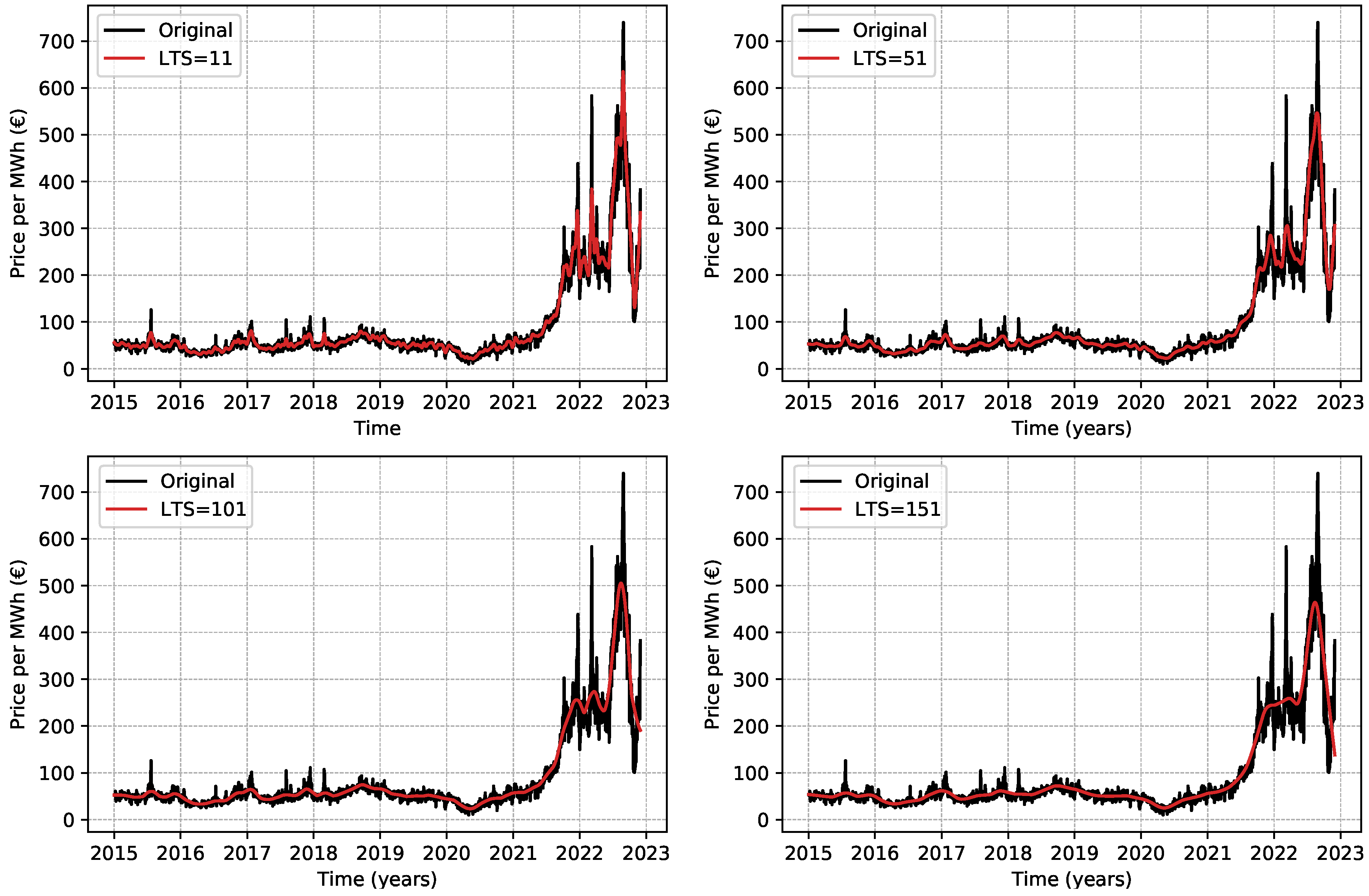
Considering these variations, the trend value was analyzed, this value was used in this paper as the observed value to forecast the electricity price. To use the trend from the STL, it is necessary to define two parameters which are the length of the seasonal smoother (LSS) and the length of the trend smoother (LTS). The results of the STL decomposition analysis are presented in Figure 4 in relation to the LTS of the time series. The variation of the value of LSS did not result in a visual change; for this reason, these results are not presented in graphical form.

To decompose the signal, it is necessary that the LTS values are odd, for this reason, the variation is presented with a step of 50 with the first value at 11, considering that it is not possible to perform the decomposition of the LTS equal to 1. From an LTS value equal to or greater than 51, the peaks were attenuated and this information was lost. Having these preliminary results, a value of LTS equal to 51 was considered the maximum possible value in the decomposition, because an abrupt decomposition causes the signal to lose its characteristics.

Considering the focus on analyzing trend variation in electricity prices, it is promising to use STL in the time series decomposition. Using the STL, oscillations are not considered and a more assertive forecast can be made based on the trend of variation of the electricity price. Based on the resulting trend signal, Facebook’s Prophet was used for forecasting.

4.2. Facebook’s Prophet

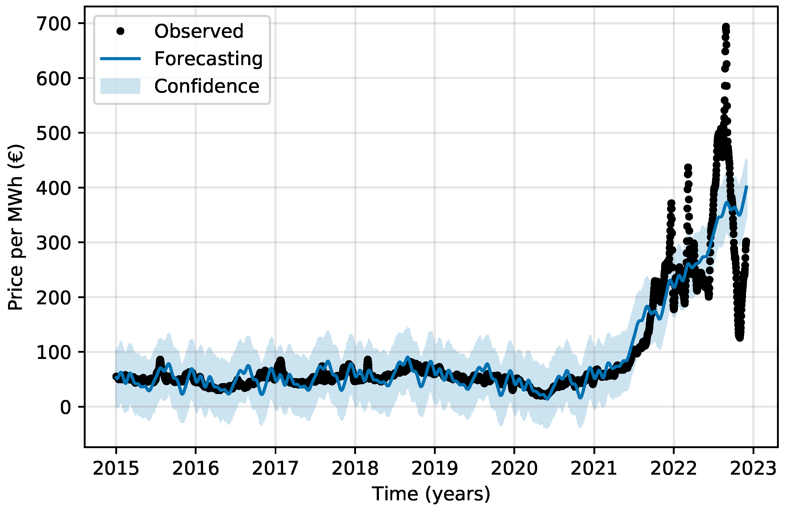
In a preliminary one-step analysis (one observation to predict), Facebook’s Prophet results in the forecast presented in Figure 5, wherein the black points are the data used to train the model, the blue line is the forecasting results, and the light blue area represents the confidence intervals.

In the analysis of the forecast about future prices, it is possible to see that there is a tendency the increase the energy bill, the big variation that occurred in the second semester of 2022 shows the volatility in the variation of the electric energy values at the beginning of winter, this variation worries the consumers since the gas value also keeps increasing. As electricity is an alternative source for heating homes in the winter in northern countries, this upward trend has a direct impact on people’s lives.

To further improve the forecasting ability, the results of the error calculation with respect to the STL decomposition are presented in

Table 1. Error evaluation regarding STL decomposition.

LTS	LSS	MSE	RMSE	MAPE (%)
11	21	8805.30	93.84	30.54
	41	8727.33	93.42	30.33
	61	8552.59	92.48	30.01
21	21	4705.48	68.60	20.56
	41	4729.80	68.77	20.59
	61	4745.27	68.88	20.63
31	21	6800.03	82.46	25.73
	41	6743.90	82.12	25.58
	61	6660.24	81.61	25.42
41	21	7178.79	84.73	26.59
	41	7070.99	84.09	26.35
	61	7035.60	83.88	26.28
51	21	8837.37	94.01	30.43
	41	8749.61	93.54	30.23
	61	8701.09	93.28	30.13

. The best error results in each LTS configuration are shown in bold, and the best overall value is shown underlined. Since an LSS lower than 21 and greater than 61 would cause the error values to increase, only the values up to this limit are presented.

When more observations are predicted relative to observed values, the model may have more difficulty predicting values with acceptable error. In a step-ahead analysis, this occurs because when a long-term evaluation is performed, the predicted values that do not match the observed reality (error) are accumulated; thus, long-term analysis is more difficult to perform when there is a high nonlinearity in the time series. However, it is possible to have a longer horizon, which in terms of energy planning is promising.

Table 2. Evaluation of the maximum observations ahead.

Observations	MSE	RMSE	MAPE (%)
1	4705.48	68.60	20.56
5	8018.98	89.54	28.49
10	13,451.76	115.98	40.10
25	32,009.12	178.91	77.71
50	61,336.33	247.66	132.61

shows the forecast error values in relation to the use of more observations.

Considering that the observations are daily, 50 observations represent having the ability to forecast the increase in the spot market price of energy 50 days ahead. In terms of market evaluation, one observation (one day ahead) would be promising for any course of action; however, when the issue of energy planning is observed, considering that electric energy is an alternative energy source to the use of gas for heating purposes, the ideal is to observe a forecast of at least 50 days, since this corresponds to the period of greatest need for heating during the winter. The STL Facebook’s Prophet results considering 50 observations are presented in Figure 6. Using 50 observations means assessing to predict the spot market value 50 days ahead.

It was observed that when many observations are used for forecasting and few for training, the model tended to have lower error results, however, the forecast shows that these results occurred because with fewer data for training the model became closer to the exponential energy increase, considering that there are political factors that influence this variation, a long term forecast does not correspond to a guarantee of accuracy, since besides market variations other factors have an influence on the long term price of electricity.

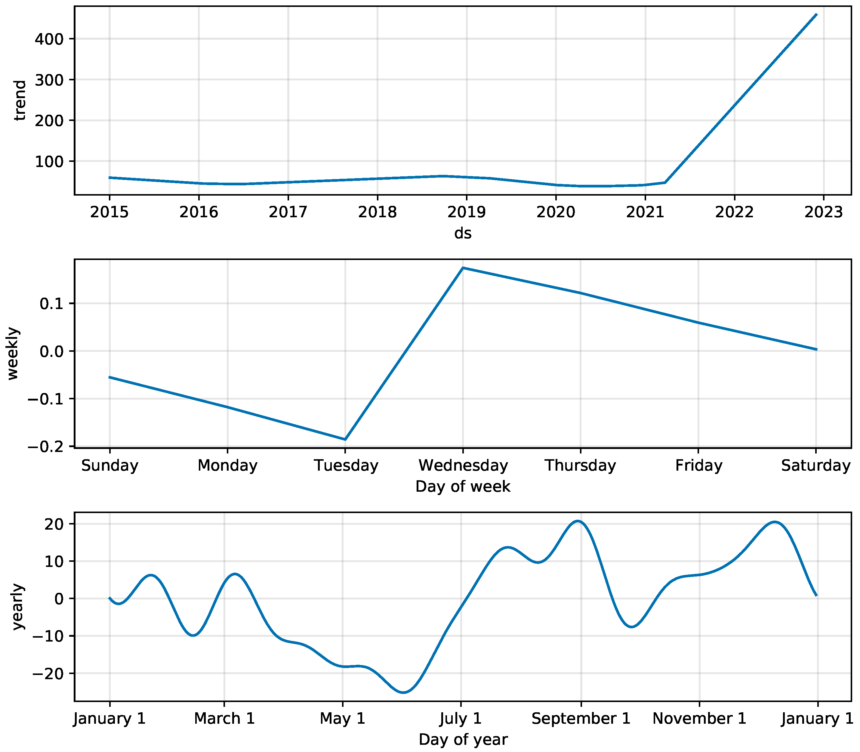
Results that are interesting in terms of model evaluation are the resulting forecast components shown in Figure 7. It can be observed that there was a trend of energy price increase from the year 2021 that was maintained in the year 2022, and based on the results obtained, it will possibly be maintained in 2023. The weekly variation shows that in the middle of the week the highest peaks of variation, with the lowest values being entered on Tuesdays. This indicates that typically the market reacts with an increase in stock purchases after a drop in its value, an expected result in relation to the stock market. The highest share price values occur in the months of September and December. This variation possibly occurs at the end of summer and the beginning of winter, which causes the market value to fluctuate considerably.

The results showed that the lowest errors in the forecast were obtained when the length of the trend smoother (LTS) was equal to 21 and the length of the seasonal smoother (LSS) was equal to 21 or 41. Specifically, the mean squared error (MSE) and root mean squared error (RMSE) values were 4705.48 and 68.60, respectively, while the mean absolute percentage error (MAPE) was 20.56%. These values represent a significant improvement over the other configurations tested, indicating that the forecast was more accurate when these parameter values were used

4.3. Discussion

The results indicate that there is a tendency for electricity prices to increase, with a particularly large variation occurring in the second semester of 2022. This increase in prices is likely due to a combination of factors, including the volatility of the energy market, the rising cost of fuel sources, and the increasing demand for electricity. The variation in prices during the winter months is of particular concern to consumers, as higher electricity prices may impact their ability to affordably heat their homes.

Our results indicated that, using an LTS of 21 and an LSS of 21, resulted in the best overall error values, with an MSE of 4705.48, an RMSE of 68.60, and a MAPE of 20.56. These findings suggest that the STL decomposition can be a useful tool for improving the accuracy of electricity price forecasting, as it allows for a more nuanced analysis of the time series data.

Overall, our analysis of the European wholesale electricity price data highlights the importance of understanding the factors that influence the formation of electricity prices and the potential benefits of utilizing statistical and machine learning techniques to make more accurate forecasts. These insights may be useful for a variety of stakeholders, including electricity generators, transmission and distribution companies, and electricity consumers, as well as policymakers seeking to optimize the functioning of the electricity market in Europe.

4.4. Short-Term Evaluation

The selection of the time window used for forecasting influences the forecast’s capability. When fewer data are observed, the model tends to require less computational effort. This issue raises a reflection on which time window is adequate to perform the market forecast, since reducing this window can lead to an improvement in the error metrics. Nevertheless, these evaluations are not representative in terms of the seasonality of the series, since longer times must be observed for a complete market evaluation.

Table 3. Evaluation of the variation in the number of days.

Time (Days)	MSE	RMSE	MAPE (%)
2890	4705.48	68.60	20.56
1825	1667.84	40.83	12.24
1460	930.85	30.50	9.14
1095	90.99	9.53	2.85
730	1406.27	37.50	11.24
365	38,681.73	196.67	58.96
180	4163.31	64.52	19.34
90	253.59	15.92	4.78

presents an evaluation of the forecasts considering variations in the time window used.

When the time window is increased, the error signal (residual) increases until it reaches its maximum (in this evaluation) at 365 observations (at which point predictions are ineffective, since the MAPE error is 58.96%). When 1095 observations are used (3 years), lower error values are found, and within this perspective, an optimization analysis could be performed to determine the optimal number of observations. Since the purpose of this paper was to evaluate the complete variation history to assess the seasonality of the variations, this was not performed. 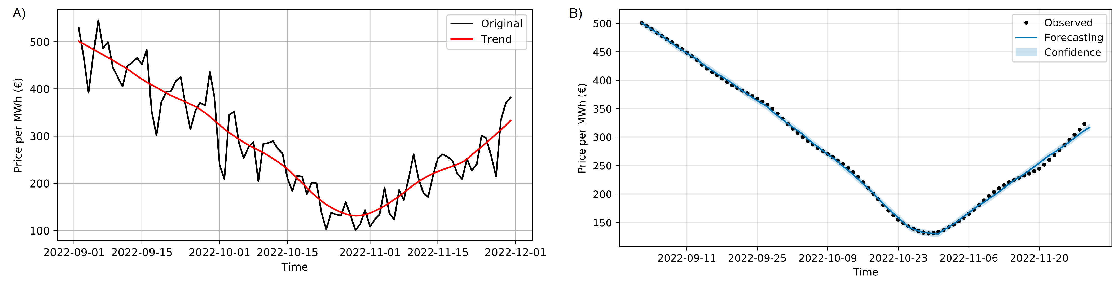Figure 8 shows the use of STL to filter the signal and Prophet to perform the forecast considering 90 observations.

The evaluation of a short period of time results in a lower forecast error of the model in view of the fact that the predictions only take into account momentary variations, and do not consider the seasonal variations of the market. In this sense using the entire dataset (with 2890 observations) is more challenging. Still, it results in an appropriate reflection of the price variation, and the energy cost scenario compared to previous years.

5. Conclusions and Future Directions of Research

In this study, we employed the decomposition ensemble forecasting paradigm, which decomposes time series data into simple components and aggregates the forecast results from all components to obtain a final forecast. We also utilized the STL technique for pre-processing the data to reduce oscillations and better understand the trends in the data. By defining appropriate values for the length of the seasonal smoother and the trend smoother, we were able to extract the trend in the data and use it as the observed value for forecasting with Facebook’s Prophet model.

Our findings showed that using STL in the decomposition of the time series can provide a better performance forecast of electricity prices in Italy by focusing on the trend of variation rather than considering oscillations as noise. This approach can be a promising tool for market participants and regulators to develop profitable strategies and ensure the security and stability of energy markets.

Future research in this area could include further exploration of different ensemble-based models and their effectiveness in forecasting electricity prices, as well as the development of improved techniques for decomposing and analyzing time series data. Additionally, further work could be undertaken to understand the impact of political and other external factors on the forecasting performance of these models. Future work can be conducted with state-of-the-art models, such as extreme gradient boosting (XGBoost) trees among other models based on ensemble learning methods that have been successfully applied by other authors.