Influence of Increasing Renewable Power Penetration on the Long-Term Iberian Electricity Market Prices

Abstract

In recent years, there has been a significant increase in investment in renewable energy sources, leading to the decarbonization of the electricity sector. Accordingly, a key concern is the influence of this process on future electricity market prices, which are expected to decrease with the increasing generation of renewable power. This is important for both current and future investors, as it can affect profitability. To address these concerns, a long-term analysis is proposed here to examine the influence of the future electricity mix on Iberian electricity prices in 2030. In this study, we employed artificial intelligence forecasting models that incorporated the main electricity price-driven components of MIBEL, providing accurate predictions for the real operation of the market. These can be extrapolated into the future to predict electricity prices in a scenario with high renewable power penetration. The results, obtained considering a framework featuring an increase in the penetration of renewables into MIBEL of up to 80% in 2030, showed that electricity prices are expected to decrease by around 50% in 2030 when compared to 2019, and there will be a new pattern of electricity prices throughout the year due to the uneven distribution of renewable electricity. The study’s findings are relevant for ongoing research on the unique challenges of energy markets with high levels of renewable generation.

1. Introduction

Over the last decades, the electricity sector has experienced critical changes in composition and operation, changing from natural monopolies to liberalized structures [1]. The integrated markets of Portugal and Spain form the Iberian electricity market, known as MIBEL, which has been operating since 2007. Within the different markets composing MIBEL, the day-ahead market is by far the most important, where almost all electrical energy is traded.

With the recent increase in renewable energy sources (RES) and their expected integration into electricity markets, some questions have arisen. One of the most important is related to future electricity prices, which are expected to decrease with the increase in RES, greatly exacerbating the so-called “missing money” problem [2,3,4]. This problem occurs when the suppliers’ revenues are not sufficient to cover all their costs, forcing market participants and future investors to change their trading strategies. Management, decision-making, and strategic planning are crucial activities in every modern business, and even more important in uncertain environments, such as the electricity market [5,6]. Therefore, it is vital to have the right forecasting tools to perform these tasks properly.

Considering the change that is expected to occur in the Iberian energy mix from today until 2030, with a projected sharp increase in the share of renewable generation, from 40% to 80–90% of the total electricity generation [7], it is important to predict how day-ahead market prices will be affected.

In this paper, a methodology is proposed concerning the development of forecasting models to assess the influence of the increasing penetration of renewable power on MIBEL spot prices for the year 2030. The results of this analysis can provide important information about future electricity market prices for both present and future investors, allowing them to make rational and thoughtful investment decisions.

A common approach when developing forecasting models, especially for short periods of time, is to use previous values of the variable under prediction, in this case, the electricity price, as input, to improve accuracy. However, this is not a feasible solution when assessing electricity prices for 2030. Therefore, a different approach was adopted, with models using only explanatory variables of the underlying process, for instance, the production of generation technologies, demand, and variable costs of fossil fuel technologies.

In the literature, different models have been proposed to perform electricity price forecasts. Weron [8] conducted an extensive and complete state-of-the-art review on the topic, evaluating the strengths and weaknesses of a variety of models and methods.

Statistical and artificial Intelligence (AI) techniques are by far the most frequently used techniques for electricity price forecasting [9,10]. With the liberalization of electricity markets in several countries, future electricity prices have become difficult to assess, and some traditional statistical methods have been considered incomplete and insufficient. The literature shows that AI algorithms, such as feedforward neural networks (FFNNs), are simple yet capable of mapping any non-linear function [10,11], making them a powerful and robust tool [8,12]. Artificial neural networks (ANNs) are frequently considered the most accurate forecasting tool when compared with traditional forecasting techniques, especially for nonstationary, nonlinear, discontinuous, and complex problems [13]. Such algorithms can easily handle nonlinear, noisy, or incomplete data due to their learning characteristics, making them a natural tool for electrical markets, considering the characteristics of electricity prices [14]. For these reasons, AI algorithms, more precisely ANNs, were used in this study.

With the increasing demand for AI models targeted at the forecasting of electricity prices, new and more sophisticated techniques have arisen. Most recently, new advancements were made regarding ANN forecasting techniques for electricity prices and stock prices, especially in the field of hybrid models. In [15], the authors proposed a hybrid kernel-based model with advanced optimization, called a kernel-based extreme learning machine. The authors used a variational-mode decomposition process to decompose the original data into its various components and a chaotic sine cosine algorithm for optimization purposes. In [16], the authors used a hybrid variational mode decomposition approach and a stacked gated recurrent unit model to predict stock prices, showing that individual stock price information/predictors are much more important than industry environment information. In [17], the authors used an empirical wavelet transform attention-based LSTM algorithm. This algorithm decomposes the initial time series into several components through the empirical wavelet transform, and then that information is processed by the attention-based and LSTM components, from which the final predictions are obtained. In [18], a whole new approach was provided. Instead of a hybrid model, the authors proposed a technique called transfer learning. A pre-trained model, from a given problem, can be optimized and used to predict electricity prices, thus increasing the model’s accuracy. However, these techniques are more suitable for shorter forecasting periods, in which the degree of uncertainty is lower than for longer time periods. More sophisticated models tend to demand more sophisticated and refined data, which is not the case for long time periods.

Electricity price forecasts can be divided into short-, medium-, and long-term, with extremely different methodologies used to address each of these time ranges. Considering the problem under consideration, and the definition provided in [8], in this study we focused on long-term electricity price forecasts.

The literature is not extensive for this particular time range, containing a relatively small number of papers and studies. One explanation for this is the uncertainty about price-driven factors in the long run, such as fuel prices, regulatory policies, political intervention, technological changes, the energy mix, grid developments, etc. Electricity price behavior in the long term is highly dependent on investments made in the power system, and on political interventions [19]. Even so, different authors have presented different methodologies and considerations when modeling and forecasting long-term electricity prices. For such a time range, more important than the model itself is the selection of the correct variables, which allow the process to be described over the long term. Several studies have proposed sets of variables and considerations that are believed to accurately describe electricity prices in the long term.

Some authors have focused more on the physical properties of the electrical market, considering variables such as the generation of energy using conventional and non-conventional technologies, imports and exports, demand, etc., and including few considerations related to the economic and social components of the market [20,21,22].

Other authors have also considered, in addition to this information, the price elasticity of electricity, gross domestic product, information about households, consumption expenditure, population data, grid connections/restrictions, new capacity installed in the future, old capacity dismissed in the future, fuel costs, CO₂ allowances, the efficiency of technologies, inflation, etc. [23,24,25].

As previously stated, the literature on electricity price forecasting in the long run is scarce, providing insufficient options to correctly assess future scenarios in which the energy mix is expected to be substantially different. To address this research gap, in this study we proposed a methodology using complex forecasting models, specifically, ANNs, with the ability to extract complex relationships from the data provided, incorporating explanatory variables that can accurately describe real market behavior and, more importantly, explanatory variables that can be extrapolated into the future and forecasted. Following this methodology, it is possible to assess future electricity prices with larger time horizons.

For that purpose, two deep learning-based ANNs, namely, feedforward neural networks (FFNNs) and long short-term memory (LSTM), were used to assess and forecast the day-ahead market prices resulting from future renewable power penetration scenarios. The use of two different forecast models allowed us to compare the experimental results and draw conclusions about their accuracy. If both models presented similar results for the simulated 2030 electricity prices, then we would be able to have an extra degree of confidence in regard to the experimental results.

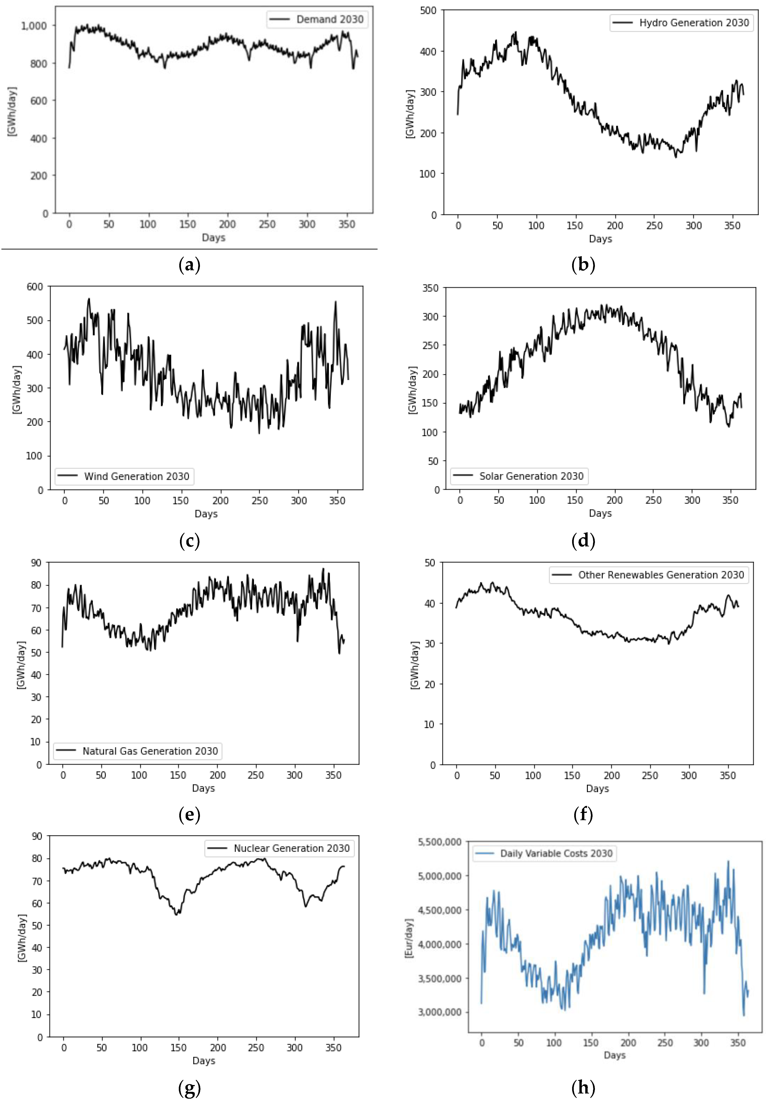
The chosen explanatory variables were the production of electricity generation technologies, demand, and variable costs, representing the physical and economic components of the market. Therefore, the final explanatory variables considered the daily electricity generation from solar, hydro, wind, other renewables, coal, natural gas, and nuclear technologies, as well as the associated fuel and CO₂ daily costs (i.e., the variable costs) and the daily demand level.

The remainder of the paper is organized as follows. In Section 2, the data sources and the applied methodology are described. Section 3 presents and discusses the experimental results in detail. Section 4 describes an ongoing study to investigate the unique challenges associated with energy markets with large-scale penetrations of renewables, placing the work described in this paper into the context of a larger goal. Finally, Section 5 presents some relevant concluding remarks.

2. Data and Methods

Data on electricity generation, energy sources, and demand were obtained from Rede Elétrica Nacional (REN) and Red Eléctrica de España (REE), the transmission system operators (TSO) for Portugal and Spain, respectively. MIBEL market prices were obtained from OMIE, the MIBEL market operator. Coal prices were obtained from the European Association for Coal and Lignite (Euracoal) and natural gas prices were obtained from Ycharts, an investment platform with information about different market stocks and prices. Information on CO₂ allowances was obtained from the European Energy Exchange market (EEX), a European platform related to all types of energy trade and the associated factors. Nuclear variable costs were collected from the Nuclear Energy Institute, directly in euros per MWh of electricity produced. All the abovementioned data were collected for the period 2015–2019, with a daily resolution.

Table 1. Yearly average prices of CO₂, coal, and natural gas for the period 2015–2019.

	2015	2016	2017	2018	2019
CO2 (EUR/ton)	7.76	5.65	5.67	16.27	24.46
Coal (EUR/ton)	61.12	62.18	87.12	91.39	64.44
Natural Gas (EUR/mmBTU)	5.8	3.88	3.86	6.52	4.08
Nuclear (EUR/MWh)	6.90	6.71	6.31	6.09	5.79
Renewable Generation (EUR/MWh)	0	0	0	0	0

summarizes the collected information concerning the yearly average prices of CO₂, natural gas, and coal. We considered both the fuel costs and CO₂ costs as variable costs.

The methodology proposed to evaluate the influence of future renewable generation on MIBEL prices comprises five steps:

• Data treatment and analysis, assessing the influence of the different components of the energy mix (demand and generation) on electricity prices.
• The construction of the two AI models (FFNN and LSTM) that will be used to predict electricity prices.
• Training and tuning of the models.
• Validation of the model.
• Modelling of the 2030 energy mix, which will be used as input to the models to obtain the simulated MIBEL electricity prices for 2030.

2.1. Data Treatment and Analysis

Having collected information about the daily demand and generation of electricity from different sources, it was then necessary to compute the associated daily CO₂ and fuel costs, which in this work were only related to natural gas and coal technologies.

To calculate the fuel costs, it was necessary to compute the daily primary energy used by natural gas and coal technologies to generate electricity. Such information can be obtained using the corresponding efficiencies. In the case of natural gas, different technologies are being considered, from combined-cycle and cogeneration systems to normal gas turbines. Accordingly, we considered it to have an average efficiency of 55%. For coal technologies, we considered the regular efficiency presented by this technology to be around 35%. With these values and the unitary fuel costs shown in Table 1, it was possible to compute the daily fuel costs. The daily CO₂ costs were computed using information about the daily emissions and the unitary price of CO₂.

A correlation analysis was performed to assess the relationship between the selected variables and the electricity prices. When discussing forecasting models it is not only important to select the correct variables, but also to assess their influence on the final output. In this way, it is possible to evaluate the coherence of future results.

According to King et. al. [26], two methods are typically used to calculate correlations between variables. If variables are normally distributed, Pearson’s correlation should be used. If not, then Spearman’s correlation should be chosen. For the specific case considered in this study, the data were not normally distributed, so Spearman’s correlation ($r_s$) was used. From $n$ samples, this correlation ranks $X_i$ and $Y_i$ variables independently, either in an ascending or descending order, and posteriorly calculates their differences ($D_i$). Using that information, the Spearman’s correlation between them is computed as follows:

$$r_s=1-\frac{6{{\displaystyle \sum }}_{i=1}^n{D}_i{}^2}{n^3-n}, D_i=X_i-Y_i$$

(1)

2.2. Construction of AI Models

Attending to the evidence found in the literature, AI models such as ANNs show an enormous potential to deal with noisy, volatile, and non-linear environments, such as the prices of the electricity market. Two ANN algorithms were used here to evaluate 2030 MIBEL electricity prices. The first was a feedforward neural network (FFNN), one of the simplest algorithms. The second is called long short-term memory (LSTM), a more complex and sophisticated algorithm that integrates the group of recurrent neural networks (RNNs).

FFNNs are the basis of deep learning [27,28,29]. This specific architecture is efficient and simple to use, and is widely applied in supervised learning. The “feedforward” designation comes from the information flux, which is processed in one direction only, from the input through the hidden layers until reaching the output, called the forward direction.

LSTM is a specific case of RNN and is considered a generalization of FFNN, with the upgrade of an internal memory. LSTM provides neurons with information feedback from the $n$ previous time steps. This means that after computing the output of a given neuron, that same information flows back into the network, and therefore the algorithm can analyze, process, and use it to compute the next output. According to Hochreiter et. al. [30], the general idea behind LSTM algorithms is to introduce the cell state, where information can be added or removed and passed to other cells. Unlike FFNN, information is propagated using unit gates (forget, input, and output gates), which are responsible for updating the cell state and computing neurons’ outputs. LSTM neurons are much more complex than the basic artificial neurons used in FFNN. According to [31,32], RNN structures may present some advantages when predicting stock prices, due to their repetitive nature, and having information on previous steps can be advantageous. When data exhibit auto-correlation or time dependence, RNNs are good candidates to extract their underlying patterns. However, that same ability to memorize previous steps may lead to some convergence and stability problems. As such, when predicting stock prices, RNNs seem to be a good candidate, but they may not always be the best ones.

In this study, both neural networks contained one input layer, two hidden layers, and one output layer. The number of input neurons was determined by the number of variables used to describe the process, namely, nine. Figure 1 shows a schematic representation of a neural network, as well as its inputs and outputs. The difference between the two algorithms consisted mainly of the information flow, meaning that in the LSTM there is the previously mentioned feedback (not represented in Figure 1).

2.3. Training the Models

In the training procedure, it is necessary to feed the models with specific data, called training data, containing predictors (or inputs) and the corresponding solutions (or targets), ensuring that they can learn, adapt, and minimize errors. Most neural networks, including the ones considered in this study, are trained by considering gradient descent techniques using the backpropagation algorithm, as described in [33,34].

In this paper, the training of the models was performed using previous information concerning the generation, demand, and variable costs considered in MIBEL for the period 2015–2019 (i.e., the variables presented in Figure 1). The forecasting strategy was implemented as a one-step ahead approach, i.e., the model predicted each daily electricity price at one time, based on the corresponding daily explanatory variables. In this way, the models could adapt to previous information and (hopefully) generalize for new cases and problems. During the training procedure, and through the implementation of an exhaustive stochastic grid search, the different hyperparameters used could be optimized. The batch size, the number of epochs, the type of optimizer, the considered cost function, the type of weight initializer, and the activation function present in the neurons are summarized in

Table 2. Hyperameter values selected after stochastic grid search optimization.

	FFNN	LSTM
Batch Size	30	30
Epochs	60	50
Optimizer	Adam	Adam
Cost Function	Root Mean Squared Error	Root Mean Squared Error
Weight Initializer	Random Uniform	Random Uniform
Activation Function	SELU	Sigmoid and Tanh

.

2.4. Validating the Models

After the construction and training of the models, it is crucial to evaluate their accuracy in generalizing for new cases (this assessment is called model validation). To perform this task, a dataset composed of predictors/inputs and targets/solutions is required, to predict and quantify the error. In this study, the plan for the validation process consisted of predicting previous MIBEL prices for each year between 2015 and 2019 and comparing the results with the known real values. When forecasting a specific year, a critical part of performing a good model validation consists in ensuring that the model cannot have access to data regarding that particular year in the training stage.

A common approach is to compare the accuracy of the models with a benchmark. In this paper, we adopted the persistence method. This method states that the value observed at time t − 1 will also occur at time t.

The error was quantified using two basic indicators: mean absolute percentage error (MAPE) and mean absolute error (MAE), as shown in (2) and (3), respectively:

$$\mathrm{MAPE}=\frac{1}{n}{\displaystyle \sum }_{\mathrm{i}=1}^n\left(\frac{Y_i-\widehat{Y_i}}{Y_i}\right)$$

(2)

$$\mathrm{MAE}=\frac{1}{n}{\displaystyle \sum }_{i=1}^n\left(Y_i-\widehat{Y_i}\right)$$

(3)

where $n$ represents the total number of samples,$\widehat{Y_i}$ is the forecasted value, and $Y_i$ is the real value.

Apart from these two indicators, a statistical analysis was also performed for a better understanding of the error, by calculating the associated statistical indicators, namely, the mean ($\mu$), standard deviation ($\sigma$), and median (M).

2.5. Modeling the Energy Mix of 2030

To forecast the electricity prices for 2030, taking into account the previously described models, it was necessary to consider information about the expected 2030 energy mix in MIBEL. In [6], the future Iberian power system was simulated using the EnergyPlan tool, following the objectives established by the European Commission and the Iberian Governments until 2040. Information about future generation technologies, electrical production, and demand is also provided in [6].

Table 3. MIBEL energy mix simulation for 2030 [7] and real values from 2019.

Technology	2019 (TWh)	2030 (TWh)	Relative Variation
Hydro	37.16	101.76	174%
Wind	67.64	123.81	83%
Solar	10.27	82.93	707%
Other Renewables	4.67	13.29	184%
Coal	17.85	0	−100%
Natural Gas	109.72	25.14	−77%
Nuclear	55.82	26.21	−53%

shows the energy mix considered for 2030, following the results of [7], and compares it with the real energy mix from 2019.

By 2030, it is clear that renewable generation will largely increase its share in MIBEL, and fossil fuel generation will be drastically reduced, with coal technologies reaching null production. For 2019, the amount of electricity originating from renewable sources, which include hydro, wind, solar, and other renewables, was around 39% of the total generation. For 2030, this percentage rises to 86%. The largest investment was observed for solar technologies, which are expected to increase their production by 707%, when compared with 2019.

The information provided in [7] was presented on a yearly basis and this needed to be converted into the models’ predictors/inputs (i.e., on a daily basis). To overcome this issue, we decided to capture past patterns of generation and demand variables and replicate them for 2030 (assuming that the distribution of predictors in 2030 would be similar to that of today). This is a simple and natural approximation. To obtain the previous patterns, one could use a single year from the 2015–2019 period or consider an average of all years in the interval. The latter approach was preferable since any unusual event that may appear in one year could be disguised by using the average of the period. Thus, an “average year” was considered.

In the computation process for daily fuel costs, we followed the same methodology as explained for previous years (2015–2019). For the computation of daily CO₂ costs, a different approach needed to be adopted, since it was not possible to access information about the daily emissions for 2030 (as was possible for previous years). To overcome this difficulty, a “natural gas emission factor” was created by dividing the total emissions from natural gas power plants by the total electricity generated for the period of 2015–2019. This allowed us to compute an average daily emission and the respective cost. This was also a simple and natural approximation which considered that the CO₂ emissions of natural gas power plants would not change in the future.

Table 4. Natural gas and CO₂ price predictions for 2030 [35].

Commodity	2030
CO2 (EUR/ton)	35
Natural Gas (EUR/mmBTU)	6

presents the CO₂ and natural gas prices, as forecasted by the Portuguese authorities in their development plans.

Figure 2 represents the used demand, generation, and variable cost distributions for the predictors in 2030.

3. Results

3.1. Correlation Analysis

Table 5. Daily correlation between generation technologies, demand, and MIBEL prices (2015–2019)—Iberian Peninsula.

Technology	Hydro	Nuclear	Coal	Natural Gas	Wind	Solar	Demand	Electricity Prices
Hydro	1
Nuclear	−0.113	1
Coal	−0.264	−0.001	1
Natural Gas	−0.346	−0.003	0.111	1
Wind	0.152	−0.023	−0.409	−0.415	1
Solar	−0.164	0.051	−0.164	0.171	−0.368	1
Demand	0.072	0.152	0.297	0.281	0.104	−0.111	1
Electricity Prices	−0.392	−0.017	0.621	0.489	−0.441	−0.081	0.276	1

and

Table 6. Hourly correlation between generation technologies, demand, and MIBEL prices (2015–2019) for Portugal only.

Technology	Hydro	Coal	Natural Gas	Wind	Solar	Demand	Electricity Prices
Hydro	1
Coal	0.175	1
Natural Gas	0.192	0.233	1
Wind	−0.132	−0.338	−0.346	1
Solar	0.097	0.056	0.314	−0.209	1
Demand	0.562	0.319	0.474	0.009	0.383	1
Electricity Prices	0.282	0.740	0.343	−0.337	0.075	0.473	1

present the results of the correlation analysis. In particular, Table 5 presents the obtained daily correlation for the period 2015–2019. Although the “other renewables” component was incorporated into the model, it was by far the least significant component of the variables under analysis and represented a mix of many different technologies incorporated into one variable. Therefore, no significant conclusions could be drawn from the correlation analysis for this variable, and thus this variable was not considered in Table 5 and Table 6.

The results of Table 5 are coherent and similar to the results of a study performed by Gelabert et. al. [36], in which the same daily correlation was also observed for MIBEL, for the period 2005–2010. It was possible to observe a positive daily correlation between fossil fuel technologies (coal and natural gas) and demand with electricity prices. This means that the days with higher generation of electricity from fossil fuel technologies and/or higher demand values were associated with higher daily market prices. On the other hand, we observed a negative correlation between renewable technologies (hydro and wind) and electricity prices. This means that the days with higher generation of electricity from renewable technologies were associated with lower market prices. Solar technology is currently a less developed technology on the market, with a small share, so its influence is also small, as represented by the low correlation factor. Nuclear technologies also exerted a small influence on the electricity market, represented by their almost null correlation with electricity prices.

The difference between these two analyses is related to hydro technologies, which in Gelabert’s results showed a positive daily correlation with electricity prices. The author justified this result by stating that this particular technology can store and shift energy to periods with higher demands and higher electricity prices (often referred to as the “strategic behavior of hydro plants”). This positive correlation reflects the positive opportunity cost of hydropower. Of course, this is highly dependent on the period of analysis, namely, on the particular market conditions observed. We recall that Gelabert’s work was applied to the period of 2005–2010, whereas the present study concerns the period 2015–2019.

For a better understanding of the problem, a more in-depth analysis was performed to capture the hourly variations. Therefore, all the information was discretized and presented on an hourly basis. Unfortunately, hourly information was only publicly available for Portugal, and therefore this correlation was built only with the Portuguese data. Despite this lack of information, the results can provide a good approximation of the reality, given the fact that Portugal and Spain are side by side, and thus when renewable resources such as wind and sun are present in Portugal, they are most likely to be available in Spain as well. It is important to note that nuclear technologies are not present in the Portuguese power system, so they were not considered in this correlation analysis. Table 6 presents the results of Spearman’s correlation analysis using Portugal’s hourly information.

This analysis provided a different overview of the interaction between market prices and energy generation technologies in the market, allowing an assessment of the relationships within each day, on an hourly basis.

Wind continued to present a negative correlation with electricity, mainly because it is a mature technology, with a considerable share of the market and bidding at prices close to 0 EUR/MWh (which induced a reduction in electricity prices). Reservoirs are dispatchable technologies, meaning that they can allocate stored energy during any period of the day. It is clear that periods with higher prices will be chosen in order to increase profits, and this strategy is reflected in the positive correlation between reservoirs and electricity prices. As stated above, solar is currently a less developed technology, with a smaller share of the energy market, meaning that its energy output is not significant during peak times, having a small influence on energy markets, which is reflected in its null or almost null correlation. Fossil fuel technologies continued to exhibit a positive correlation with electricity prices, as expected.

Based on both analyses, it is possible to state that, in general, an increase in renewable generation tended to decrease the average daily market price, and an increase in fossil fuel generation and demand levels tended to increase market prices. It is also possible to state that hydro technologies showed an hourly positive opportunity cost, represented by the positive hourly correlation with electricity prices, although this does not necessarily mean that such technologies increased market prices. In fact, an increase in hydro generation tended to decrease electricity prices, which was indicated by a negative daily correlation. These conclusions are coherent with those of other studies in the literature which addressed the same topic [37,38,39].

3.2. Model Validation

The validation process consisted of predicting previous years of MIBEL electricity prices, for the period of 2015 to 2019, and comparing them with the real values. This prediction process was carried out using the two aforementioned forecasting models (FFNN and LSTM) and the list of explanatory variables depicted in Figure 2. The results ere also compared by means of the benchmark persistence method.

Table 7. Yearly forecasting error values of the FFNN, LSTM, and persistence methods.

Year	FFNN		LSTM		Persistence
	MAPE (%)	MAE (EUR/MWh)	MAPE (%)	MAE (EUR/MWh)	MAPE (%)	MAE (EUR/MWh)
2015	10.63	4.93	10.49	4.53	13.60	6.14
2016	21.32	5.11	18.83	4.43	17.80	4.87
2017	8.95	4.72	8.01	4.33	8.70	4.00
2018	11.52	4.63	11.03	4.55	10.50	4.14
2019	10.68	5.03	10.52	4.32	11.00	4.49

shows the results obtained using the MAPE and MAE accuracy indicators.

The results of the ANN simulations showed MAPE values between 8% and 11.5%, corresponding to MAE values between 4.32 EUR/MWh and 5.11 EUR/MWh, except for 2016, which exhibited higher MAPE values. Two conclusions may be drawn from Table 7. The first corresponds to the high MAPE observed for the year 2016. However, when analyzing the absolute error (MAE), we found that the results were very similar for the remaining years. The high MAPE occurred because, for this particular year, unusual variability and price singularities were present, which imposed some limitations on the ability of the models to accommodate such singularities. Furthermore, and most importantly, the model registers several real electricity prices that were close to zero, which led to a sharp increase in the MAPE values. Therefore, the extremely high MAPE values registered on some days increased the overall MAPE value for these particular years. This effect was not verified for the rest of the years in the 2015–2019 period.

The second conclusion that could be drawn was that, in general, the ANN-based models (FFNN and LSTM) performed worse than the persistence model. This was due to the limitations imposed by the proposed model, which used correlated explanatory variables instead of the past values of the variables being predicted. As stated above, it is a common approach, in forecasting models, to use previous information about the variable being predicted (electricity prices) as the input of the model, allowing better accuracy. This was not possible to implement for 2030 forecasts but it was possible for the 2015–2019 predictions. In this way, a new simulation was performed by introducing the market price of the last n days as an explanatory variable, in addition to production technologies, demand, and variable costs. After performing several experiments, we concluded that the optimum number of previous days, which led to the minimum error, was equal to five. This means that the new models used demand, generation, and variable costs from day n, as well as electricity prices from the days n − 1, n − 2, …, n − 5, to predict electricity prices at day n. To distinguish these from the previous cases, these new models were named “FFNN 5 days” and “LSTM 5 days”. The forecasting procedure and interval were the same as those used in the FFNN and LSTM algorithms. The results of this analysis were also compared with the benchmark values and are shown in

Table 8. Yearly forecasting error values of the FFNN 5 days, LSTM 5 days, and persistence methods.

Year	FFNN 5 Days		LSTM 5 Days		Persistence
	MAPE (%)	MAE (EUR/MWh)	MAPE (%)	MAE (EUR/MWh)	MAPE (%)	MAE (EUR/MWh)
2015	8.82	3.82	8.51	3.67	13.60	6.14
2016	14.30	3.51	13.60	3.43	17.80	4.87
2017	7.14	3.66	6.84	3.54	8.70	4.00
2018	8.72	3.34	8.56	3.21	10.50	4.14
2019	8.54	3.89	8.45	3.53	11.00	4.49

.

The results for the new simulations exhibited MAPE values between 7% and 9%, corresponding to MAE values between 3.34 EUR/MWh and 3.89 EUR/MWh, except for 2016, which exhibited a MAPE value of around 14%. It was possible to observe a decrease in the overall error when using the “FFNN 5 days” and “LSTM 5 days” models, when comparing their results with those of FFNN and LSTM. We also verified that the new models outperformed the benchmark, which did not occur when using the previous models. This means that the inclusion of previous daily prices as an explanatory variable improved the accuracy of the models, although it would not be a feasible solution to predict 2030 electricity prices. On the other hand, it was not possible to use the persistence method to assess electricity prices for 2030.

We thus proved that the proposed models could forecast the market prices relatively well and represent a viable solution for the prediction of electricity prices for 2030.

Apart from the MAPE and MAE evaluations, a statistical analysis of the errors was also conducted. Statistical indicators, such as the mean ($\mathsf{\mu }$), standard deviation ($\mathsf{\sigma }$), and median (M), are presented in

Table 9. Statistical error indicators—mean ($\mathsf{\mu }$), standard deviation ($\mathsf{\sigma }$), and median (M), in EUR/MWh, for FFNN and LSTM errors.

Year	FFNN			LSTM
	$\mathcal{\mu }$	$\mathcal{\sigma }$	M	$\mathcal{\mu }$	$\mathcal{\sigma }$	M
2015	0.67	5.29	1.68	−0.69	5.48	−1.45
2016	−2.53	6.00	−2.52	−2.51	5.47	−2.49
2017	2.25	5.83	2.07	0.94	6.24	−0.26
2018	2.60	5.67	3.22	2.46	5.16	3.03
2019	0.99	5.26	0.7	0.49	5.15	0.88

.

The statistical error values were similar for both neural networks, as expected, given all the previous evidence. In a general way, it is possible to state that errors were somewhat normally distributed, with mean values close to zero. This information provides confidence and security in regard to the models. If the errors had all been either positive or negative, then the neural networks would probably have been biased or over-fitted in regard to some parameters.

3.3. Electricity Market Prices for 2030

The following analysis is divided into two parts. In the first, the annual average values of the simulated forecasted electricity prices for 2030 are assessed. In the second, the pattern of the simulated electricity prices for 2030 is evaluated. Although the accuracy of the models has been assessed and compared in the above sections, such statements and assessments are no longer valid, or even possible, when forecasting electricity prices for the future (the 2030 horizon), since no real values are available for comparison.

3.3.1. Annual Average Electricity Price for 2030

This analysis addresses how the energy mix predicted for 2030 affects the MIBEL yearly mean electricity price.

Table 10. Forecasted annual average electricity price for 2030 in MIBEL.

Neural Network	Average Price 2030 (EUR/MWh)
FFNN	22.94
LSTM	25.32

presents the forecasted average electricity price for 2030, using both models, FFNN and LSTM.

A slight difference of 2.38 EUR/MWh could be observed in the annual average prices forecasted by the two algorithms. Such a difference was expected and can be considered irrelevant since both values are of the same order of magnitude.

The results showed a general reduction in the average price for 2030 when compared with that from any year from the 2015–2019 period (as shown in

Table 11. Annual average MIBEL electricity prices in the 2015–2019 period.

Year	Average Price in MIBEL (EUR/MWh)
2015	50.32
2016	39.66
2017	52.24
2018	57.29
2019	47.68

).

The observed reduction can be explained by the expected large increase in renewable electricity production and the associated decrease in the fossil fuel contribution in 2030. This is in line with previous findings, which stated that an increase in renewable electricity production, with zero or near-zero variable costs, tends to decrease market prices, as well as leading to the replacement of fossil fuel technologies with high marginal costs.

3.3.2. Annual Electricity Price Distribution for 2030

It was important to assess the behavior of the forecasted values throughout the year 2030 and to understand whether the general pattern differed or not from that of the previous period. In a positive case, it is important to analyze the reasons for such behavior. Figure 3 and Figure 4 provide overviews of the yearly electricity price distribution for 2030, based on the results of the FFNN and LSTM algorithms, respectively.

Both figures show that there was consistency and similarity in the price distribution throughout the year, with valley prices corresponding to the winter and spring periods, and spike prices corresponding to the summer and autumn periods.

For 2030, we observed a new pattern for electricity prices, when compared with that of 2019 (for instance). Indeed, in 2019 (and in previous years), daily average prices tended to oscillate around a mean, as shown in Figure 5. For 2030, the behavior was slightly different, with several months of electricity prices below and above the mean, as shown in Figure 6.

It is important to understand the factors that led to such results. For that purpose, and considering the fact that electricity market prices are dependent on marginal costs, the relationship between renewable and non-renewable generation and the forecasted electricity prices were assessed. We considered only the results of the FFNN method, but these conclusions are also applicable to the LSTM algorithm.

Figure 7 shows the relationship between the forecasted FFNN electricity prices and the levels of renewable energy generation. Figure 8 and Figure 9 provide information about the comparison between renewable and fossil fuel production, and between fossil fuel production and forecasted FFNN electricity prices, respectively.

In Figure 7, an inverse relationship can be observed between electricity prices and renewable energy generation, with periods of higher renewable production presenting lower prices, and periods of lower renewable production presenting higher prices. Figure 8 displays a negative correlation between renewable and fossil fuel generation, i.e., in periods of higher renewable generation, fossil fuel technologies reduced their energy output and vice-versa. Moreover, Figure 9 shows that periods with higher market prices were directly connected with periods of higher fossil fuel generation, in this case, natural gas, due to the higher marginal costs.

This analysis clarifies why 2030 exhibited a different electricity price pattern throughout the year, compared with the earlier period. This was mainly due to the large-scale installed capacity of renewable energies for 2030, which resulted in an uneven distribution of renewable electricity throughout the year, as shown in Figure 7 and Figure 8. Since electricity prices were highly related to the energy mix, the uneven renewable distribution also induced an uneven electricity price distribution throughout the year, i.e., periods with high renewable production corresponded to low electricity prices and vice-versa.

4. Market Design and the Missing-Money Problem

Electricity markets (EMs) are built on well-established rules of transparency and competition. For the specific case of European markets, the ‘common’ design framework includes day-ahead and intra-day-markets, operating together with forward markets and complemented with balancing markets (see, e.g., [40,41,42]). This framework was developed, however, when the majority of power plants were fuel-based, meaning that their production could be controllable, with a limited economic impact.

The clean energy transition creates unique challenges in the design and operation of electricity markets. Chief among these is the well-known missing-money problem—the concern that even robust EMs may not provide sufficient incentives for at least some generators to earn revenue to pay for both variable and fixed costs [5]. In other words, the concern is that insufficient incentives for generators to build new capacity (or even maintain existing capacity) will result in insufficient installed capacity to serve the required loads, particularly during peak periods.

Most existing market designs already incorporate at least two mechanisms to meet this challenge: scarcity pricing and forward capacity markets. Scarcity pricing can be based on the value of lost load pricing, ancillary service scarcity pricing, or even emergency demand-response pricing. This allows energy prices to rise above the variable cost of the most expensive operating resources when the system is capacity-constrained. Although difficult to predict in terms of investment in capital, these prices may provide important revenue for resources to recover fixed capital costs (see, e.g., [3]).

However, energy-only markets—that is, markets based on scarcity pricing or a similar mechanism—have been the subject of a somewhat intense debate. In particular, some industry members and researchers have made strong arguments that they cannot incentivize appropriate investments, stating the need for additional incentive mechanisms and highlighting the importance of forward capacity markets. These markets determine capacity prices depending on the current supply of capacity and predicted capacity needs. They look ahead to ensure that sufficient capacity will be available to meet load requirements, especially in peak periods, and aim to provide important incentives for new capacity to be built in locations where it is most needed (see, e.g., [3]).

With the increasing penetration of renewable energy generation—which is likely to offer electricity at very low costs—both the average energy prices and the cleared energy levels of power plants are likely to be reduced. This, in turn, could reduce the overall revenue for generators, and therefore may (greatly) exacerbate the missing-money problem.

At present, it is unclear whether or not the ‘common’ design framework provides the right incentives to support the issues of resource adequacy and revenue sufficiency in future power systems with large-scale penetration by renewables. Accordingly, there is a pressing need to monitor the impacts of such large penetrations on existing markets to determine if the ‘common’ framework is still effective. If it leads to inefficiency, increased market power, reduced competition, or a degradation in reliability, important modifications may be required, or a new design framework may even be necessary.

In our ongoing studies, we are examining the use of an agent-based tool to help manage the unique challenges of EMs with large-scale penetration by renewables. The tool is called MATREM (for multi-agent trading in electricity markets) [43]. In this research, we aim to investigate emerging and new market design elements to ensure that the resources needed to meet future reliability requirements have adequate opportunities to recover their costs. To this end, the feasibility of energy-only markets will be investigated, together with studies of evolving capacity mechanisms and the main new design elements.

The plan involves the use of an iterative procedure to search for operational practices in relation to market design—that is, various elements of market design will be investigated, implemented, and evaluated iteratively until a consensus emerges on specific best practices. Put differently, the MATREM system will be extended with specific market design elements and the empirical evaluation of such elements will be performed by considering a number of forward-looking scenarios (for the years 2030 and 2050). In this way, the work presented in this paper constitutes part of a larger project plan and represents an important step towards one of its major goals.

5. Conclusions

According to the information collected in this study, from 2019 until 2030, the share of renewable electricity in MIBEL is expected to increase, from 39% up to 86% of the total electrical generation, driven by the continuous increase in the installed renewable capacity. The main goal of this study was to evaluate the influence of increasing renewable power penetration on future MIBEL prices, with a special focus on 2030. The developed models based on artificial intelligence, namely, the feedforward neural network (FFNN) and long short-term memory (LSTM) algorithms, were constructed using explanatory variables of the underlying process. The chosen variables were the production of electricity generation technologies, demand, and fossil fuel variable costs, which represented the physical and economic components of the market.

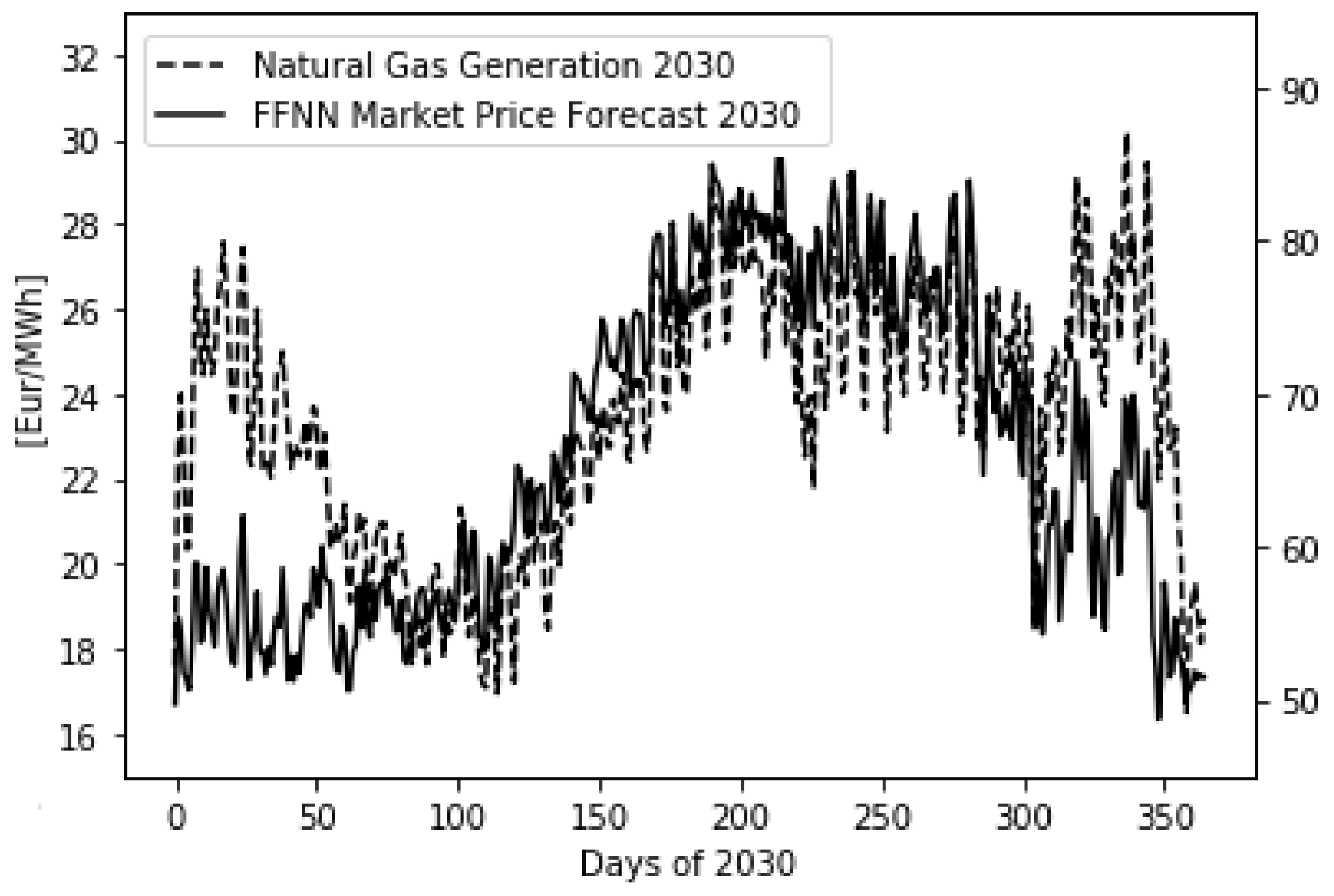
Both a daily and hourly correlation between generation, demand, and electricity prices was developed for the period 2015–2019 in order to assess their influence on electricity prices. The results showed that an increase in renewable generation tended to decrease the average daily market price and an increase in fossil fuel generation and demand levels tended to increase market prices. Moreover, hydro technologies exhibited a positive opportunity cost, represented by their positive hourly correlation with electricity prices. However, on a wider scale, an increase in hydro generation tended to decrease electricity prices, which was shown by a negative daily correlation.

To validate the models, the FFNN and LSTM algorithms were used to forecast the of MIBEL electricity prices of previous years (2015–2019), and their errors were compared with a benchmark. The results showed similarity between the two AI models and the benchmark, with MAPE and MAE values around 8–11.5% and 4.32–5.11 EUR/MWh, respectively. The similarity in the accuracy of both algorithms and the benchmark can be explained by the fact that no past electricity prices were used; rather, only explanatory variables related to the process were used. To justify this statement, another model was constructed, which, in addition to the previous inputs, also used information about the last n days of electricity prices, more precisely from the last 5 days. The results showed that these models, with the extra inputs, showed improved accuracy and outperformed the benchmark model, with MAPE and MAE values between 6.84–8.81% and 3.21–3.89 EUR/MWh, respectively. Accordingly, FFNN and LSTM provided reasonable values of accuracy and thus represented a viable solution for the problem under study.

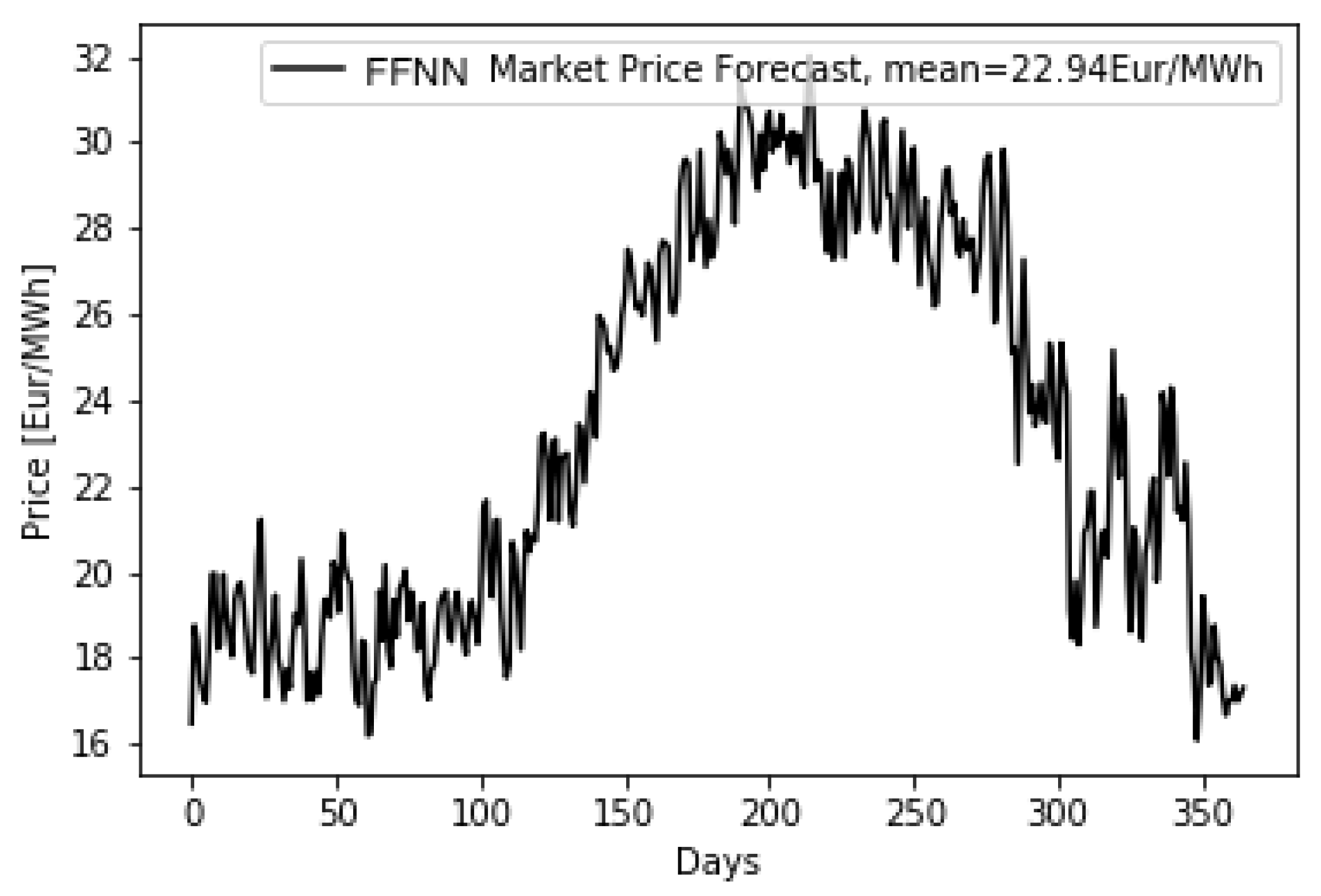
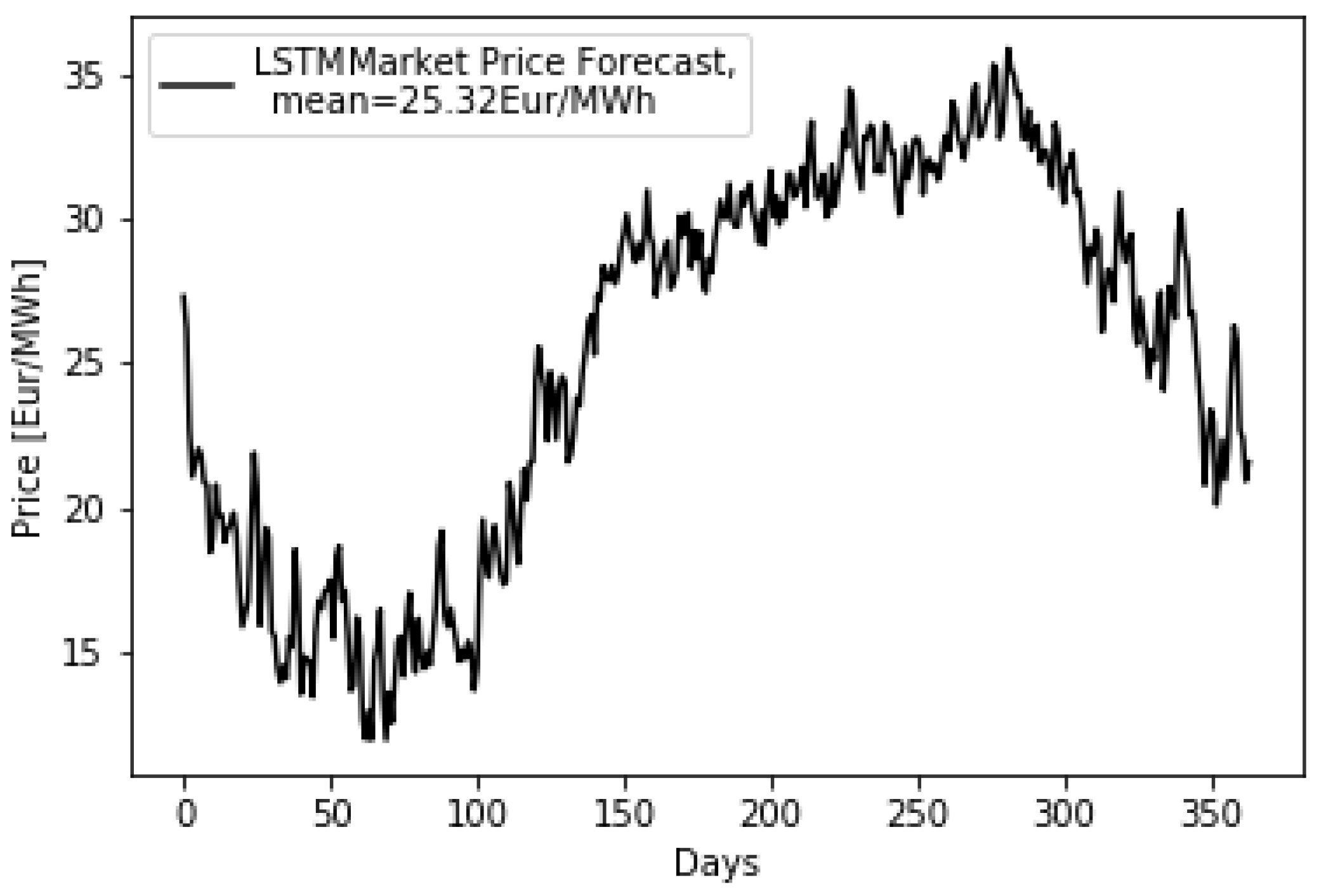
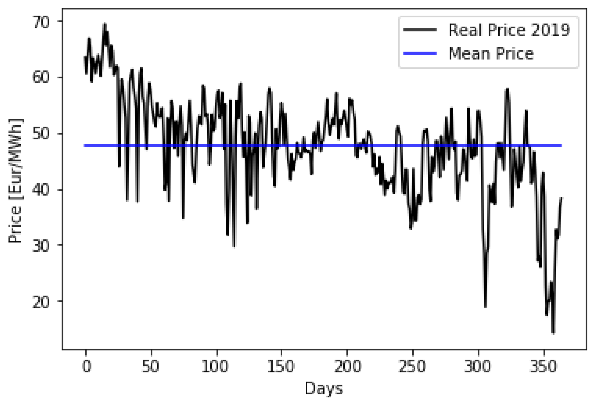
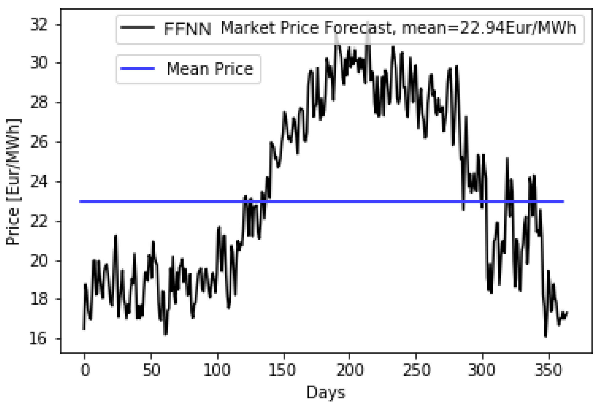
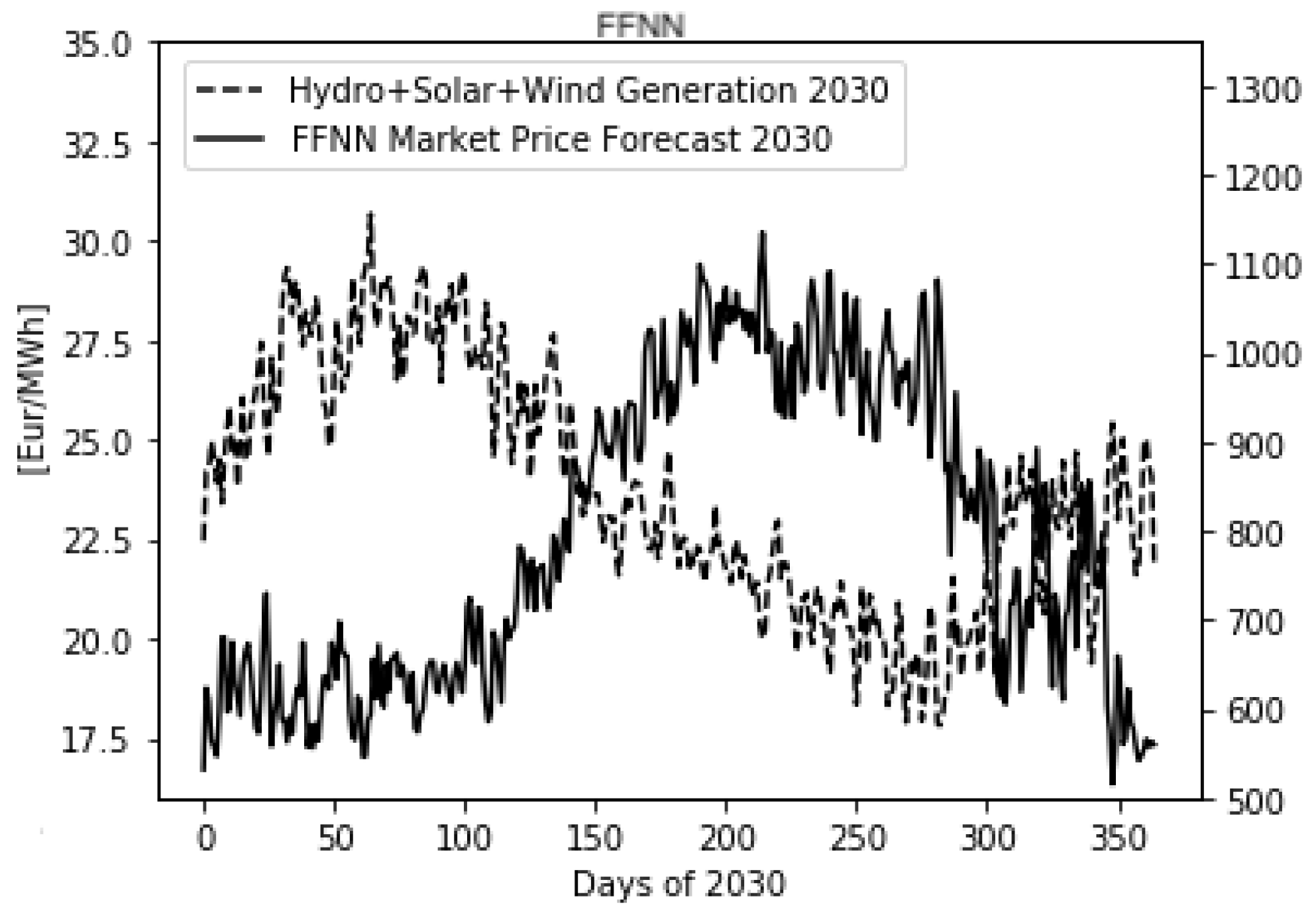
Regarding the prediction of the 2030 electricity prices in MIBEL, a large reduction in the annual average electricity price for 2030, with values of 22.94 EUR/MWh and 25.32 EUR/MWh for the FFNN and LSTM algorithms, respectively, was found. In comparison with 2019 (with an average electricity price of 47.68 EUR/MWh), the forecasted values corresponded to a relative reduction of about 50%. This is a substantial reduction, compatible with the expected high levels of renewable generation in 2030, with near-zero variable costs. Another finding was that the forecasted electricity prices presented a different pattern throughout the year, as compared with the 2019 calendar year, for instance. The effect of the drastic change in the energy mix composition predicted for 2030 was reflected in the distribution of electricity prices throughout the year, which closely followed the inverse pattern of renewable production.

References

1. Ciarreta, A.; Nasirov, S.; Silva, C. The development of market power in the Spanish power generation sector: Perspectives after market liberalization. Energy Policy 2016, 96, 700–710. [Google Scholar] [CrossRef]
2. Newbery, D. Missing money and missing markets: Reliability, capacity auctions and interconnectors. Energy Policy 2016, 94, 401–410. [Google Scholar] [CrossRef] [Green Version]
3. Lopes, F.; Coelho, H. Electricity Markets with Increasing Levels of Renewable Generation: Structure, Operation, Agent-Based Simulation and Emerging Designs; Springer International Publishing: Cham, Switzerland, 2018. [Google Scholar]
4. Ciarreta, A.; Espinosa, M.P.; Pizarro-Irizar, C. Has renewable energy induced competitive behavior in the Spanish electricity market? Energy Policy 2017, 104, 171–182. [Google Scholar] [CrossRef]
5. Stoft, S. Power System Economics: Designing Markets for Electricity; IEEE Press Wiley-Interscience: Hoboken, NJ, USA; John Wiley & Sons, Inc. Publication: Hoboken, NJ, USA, 2002. [Google Scholar]
6. Shahidehpour, M. Market Operations in Electric Power Systems: Forecasting, Scheduling and Risk Management; IEEE Press Wiley-Interscience: Hoboken, NJ, USA; John Wiley & Sons, Inc. Publication: Hoboken, NJ, USA, 2002. [Google Scholar]
7. Pereira, G.M. Simulation of the Future Iberian Power System Till 2040. Master’s Thesis, Técnico Lisboa, University of Lisbon, Lisbon, Lisbon, Portugal, 2020. [Google Scholar]
8. Weron, R. Electricity price forecasting: A review of the state-of-the-art with a look into the future. Int. J. Forecast. 2014, 30, 1030–1081. [Google Scholar] [CrossRef] [Green Version]
9. Ugurlu, U.; Oksuz, I.; Tas, O. Electricity Price Forecasting Using Recurrent Neural Networks. Energies 2018, 11, 1255. [Google Scholar] [CrossRef] [Green Version]
10. Hornik, K.; Stinchcombe, M.; White, H. Multilayer feedforward networks are universal approximators. Neural Netw. 1989, 2, 359–366. [Google Scholar] [CrossRef]
11. Funahashi, K.-I. On the approximate realization of continuous mappings by neural networks. Neural Netw. 1989, 2, 183–192. [Google Scholar] [CrossRef]
12. Ranjbar, M.; Soleymani, S.; Sadati, N.; Ranjbar, A.M. Electricity Price Forecasting Using Artificial Neural Network. In Proceedings of the in 2006 International Conference on Power Electronics, Drives and Energy Systems, New Delhi, India, 12–15 December 2006; pp. 1–5. [Google Scholar] [CrossRef]
13. Hobbs, B.F.; Helman, U.; Jitprapaikulsarn, S.; Konda, S.; Maratukulam, D. Artificial neural networks for short-term energy forecasting: Accuracy and economic value. Neurocomputing 1998, 23, 71–84. [Google Scholar] [CrossRef]
14. Tang, Z.; Fishwick, P.A. Feedforward Neural Nets as Models for Time Series Forecasting. INFORMS J. Comput. 1993, 5, 374–385. [Google Scholar] [CrossRef]
15. Yang, W.; Sun, S.; Hao, Y.; Wang, S. A novel machine learning-based electricity price forecasting model based on optimal model selection strategy. Energy 2021, 238, 121989. [Google Scholar] [CrossRef]
16. Zhu, Q.; Che, J.; Li, Y.; Zuo, R. A new prediction NN framework design for individual stock based on the industry environment. Data Sci. Manag. 2022, 5, 199–211. [Google Scholar] [CrossRef]
17. Peng, L.; Wang, L.; Xia, D.; Gao, Q. Effective energy consumption forecasting using empirical wavelet transform and long short-term memory. Energy 2021, 238, 121756. [Google Scholar] [CrossRef]
18. Yang, H.; Schell, K.R. Real-time electricity price forecasting of wind farms with deep neural network transfer learning and hybrid datasets. Appl. Energy 2021, 299, 117242. [Google Scholar] [CrossRef]
19. Sisodia, G.S. Methodology for Electricity Price Forecasting in the Long Run. Energy Procedia 2016, 95, 195–199. [Google Scholar] [CrossRef] [Green Version]
20. Kotur, D.; Mileta, Ž. Neural network models for electricity prices and loads short and long-term prediction. In Proceedings of the 4th International Symposium on Environmentally Friendly Energies and Applications (EFEA), Belgrade, Serbia, 14–16 September 2016. [Google Scholar]
21. Azofra, D.; Martínez, E.; Jiménez, E.; Blanco, J.; Azofra, F.; Saenz-Diaz, J.C. Comparison of the influence of photovoltaic and wind power on the Spanish electricity prices by means of artificial intelligence techniques. Renew. Sustain. Energy Rev. 2015, 42, 532–542. [Google Scholar] [CrossRef]
22. Yousefi, A.; Sianaki, O.A.; Sharafi, D. Long-Term Electricity Price Forecast Using Machine Learning Techniques. In Proceedings of the IEEE Innovative Smart Grid Technologies—Asia (ISGT Asia), Chengdu, China, 24 May 2019; pp. 2909–2913. [Google Scholar] [CrossRef]
23. Pohv, M.; Fleten, S.E. Modeling Long-Term Electricity Forward Prices. IEEE Trans. Power Syst. 2009, 24, 1649–1656. [Google Scholar]
24. Pohv, M.; Golob, R.; Fleten, S.E. Modelling the Structure of Long-Term Electricity Forward Prices at Nord Pool. In Handbook of Power Systems II; Rebennack, S., Pardalos, P.M., Pereira, M.V., Iliadis, N.A., Eds.; Springer: Berlin/Heidelberg, Germany, 2010; pp. 189–212. [Google Scholar]
25. Azadeh, A.; Moghaddam, M.; Mahdi, M.; Seyedmahmoudi, S.H. Optimum Long-Term Electricity Price Forecasting in Noisy and Complex Environments. Energy Sources Part B Econ. Plan. Policy 2013, 8, 235–244. [Google Scholar] [CrossRef]
26. King, A.P.; Eckersley, R.J. Descriptive Statistics II: Bivariate and Multivariate Statistics. In Statistics for Biomedical Engineers and Scientists; Academic Press: London, UK, 2019; pp. 23–56. [Google Scholar] [CrossRef]
27. LeCun, Y.; Bengio, Y.; Hinton, G.E. Deep learning. Nature 2015, 521, 436–444. [Google Scholar] [CrossRef]
28. Goodfellow, I.; Bengio, Y.; Courville, A. Deep Learning; MIT Press: Cambridge, MA, USA, 2016. [Google Scholar]
29. Charniak, E. Introduction to Deep Learning; MIT Press: Cambridge, MA, USA, 2018. [Google Scholar]
30. Hochreiter, S.; Schmidhuber, J. Long Short-Term Memory. Neural Comput. 1997, 9, 1735–1780. [Google Scholar] [CrossRef]
31. Brezak, D.; Bacek, T.; Majetic, D.; Kasac, J.; Novakovic, B. A comparison of feed-forward and recurrent neural networks in time series forecasting. In Proceedings of the 2012 IEEE Conference on Computational Intelligence for Financial Engineering & Economics (CIFEr), New York, NY, USA, 29–30 March 2012; pp. 1–6. [Google Scholar]
32. Dematos, G.; Boyd, M.S.; Kermanshahi, B.; Kohzadi, N.; Kaastra, I. Feedforward versus recurrent neural networks for forecasting monthly japanese yen exchange rates. Asia-Pac. Financ. Eng. Jpn. Mark. 1996, 3, 59–75. [Google Scholar] [CrossRef]
33. Géron, A. Hands-on Machine Learning with Scikit-Learn, Keras, and TensorFlow: Concepts, Tools, and Techniques to Build Intelligent Systems; O’Reilly Media: Sebastopol, CA, USA, 2019. [Google Scholar]
34. Amari, S.-I. Backpropagation and stochastic gradient descent method. Neurocomputing 1993, 5, 185–196. [Google Scholar] [CrossRef]
35. RNC2050. Roadmap for Carbon Neutrality 2050. Available online: https://www.portugal.gov.pt/download-ficheiros/ficheiro.aspx?v=%3d%3dBAAAAB%2bLCAAAAAAABACzMDexBAC4h9DRBAAAAA%3d%3d (accessed on 19 March 2020).
36. Gelabert, L.; Labandeira, X.; Linares, P. An ex-post analysis of the effect of renewables and cogeneration on Spanish elec-tricity prices. Energy Econ. 2011, 33, S59–S65. [Google Scholar] [CrossRef]
37. Pereira, J.P.; Pesquita, V.; Rodrigues, P.M.M. The effect of hydro and wind generation on the mean and volatility of electricity prices in Spain. In Proceedings of the 14th International Conference on the European Energy Market (EEM), Dresden, Germany, 9 June 2017; pp. 1–8. [Google Scholar] [CrossRef]
38. Azofra, D.; Martínez, E.; Blanco, J.; Saenz-Díez, J.C. Comparison of the influence of biomass, solar–thermal and small hydraulic power on the Spanish electricity prices by means of artificial intelligence techniques. Appl. Energy 2014, 121, 28–37. [Google Scholar] [CrossRef] [Green Version]
39. Mosquera-López, S.; Uribe, J.M.; Manotas-Duque, D.F. Effect of stopping hydroelectric power generation on the dynamics of electricity prices: An event study approach. Renew. Sustain. Energy Rev. 2018, 94, 456–467. [Google Scholar] [CrossRef]
40. Nord Pool. The Nordic Electricity Exchange. Available online: https://www.nordpoolspot.com/ (accessed on 10 May 2021).
41. EPEX SPOT. The European Power Exchange. Available online: http://www.epexspot.com/en (accessed on 10 May 2021).
42. MIBEL. The Iberian Market. Available online: http://mibel.com/en/home_en/ (accessed on 10 May 2021).
43. Lopes, F. MATREM: An Agent-based Simulation Tool for Electricity Markets. In Electricity Markets with Increasing Levels of Renewable Generation: Structure, Operation, Agent-Based Simulation and Emerging Designs; Springer: Cham, Switzerland, 2018; pp. 189–225. [Google Scholar]
Figure 1. Schematic representation of the ANNs.
Energies 16 01054 g001
Figure 2. Daily demand, generation, and variable costs for 2030. (a) Daily demand for 2030; (b) daily hydro generation for 2030; (c) daily wind generation for 2030; (d) daily solar generation for 2030; (e) daily natural gas generation for 2030; (f) daily generation by other renewables for 2030; (g) daily nuclear generation for 2030; (h) daily variable costs for 2030.
Energies 16 01054 g002
Figure 3. Forecasted electricity prices for 2030 in MIBEL, determined using FFNN.
Energies 16 01054 g003
Figure 4. Forecasted electricity prices for 2030 in MIBEL, determined using LSTM.
Energies 16 01054 g004
Figure 5. Eeal electricity prices in MIBEL for 2019 and the yearly average price.
Energies 16 01054 g005
Figure 6. Forecasted electricity prices in MIBEL for 2030 and the yearly average price.
Energies 16 01054 g006
Figure 7. Forecasted FFNN electricity prices versus hydro, solar, and wind power generation (renewables) for 2030 in MIBEL.
Energies 16 01054 g007
Figure 8. Hydro, solar, and wind (renewables) versus natural gas generation for 2030 in MIBEL.
Energies 16 01054 g008
Figure 9. Natural gas generation versus forecasted FFNN electricity prices for 2030 in MIBEL.
Energies 16 01054 g009