Optimal Power Flow Solution for Bipolar DC Networks Using a Recursive Quadratic Approximation

Abstract

The problem regarding of optimal power flow in bipolar DC networks is addressed in this paper from the recursive programming stand of view. A hyperbolic relationship between constant power terminals and voltage profiles is used to resolve the optimal power flow in bipolar DC networks. The proposed approximation is based on the Taylors’ Taylor series expansion. In addition, nonlinear relationships between dispersed generators and voltage profiles are relaxed based on the small voltage voltage-magnitude variations in contrast with power output. The resulting optimization model transforms the exact nonlinear non-convex formulation into a quadratic convex approximation. The main advantage of the quadratic convex reformulation lies in finding the optimum global via recursive programming, which adjusts the point until the desired convergence is reached. Two test feeders composed of 21 and 33 buses are employed for all the numerical validations. The effectiveness of the proposed recursive convex model is verified through the implementation of different metaheuristic algorithms. All the simulations are carried out in the MATLAB programming environment using the convex disciplined tool known as CVX with the SEDUMI and SDPT3 solvers.

1. Introduction

Bipolar DC distribution networks are emerging technologies based on the well-known bipolar configuration HVDC transmission lines [1], where two poles are used to increase the power transference capabilities of the system [2,3]. In the case of bipolar DC distribution grids, the typical configuration employed is composed of three conductors marketed as positive $\left(p\right)$, negative $\left(n\right)$, and neutral $\left(o\right)$. Additionally, there is the possibility of connecting monopolar loads (loads connected between one of the positive or negative poles and the neutral one). B and bipolar loads (i.e., connections between the positive and the negative pole) [4,5]. There are three main important characteristics: (i) the bipolar DC configuration can transfer double of energy in comparison with a monopolar DC configuration by increasing about 33.33% the initial investment by with the inclusion of an additional conductor along the grid topology [6]; (ii) the presence of multiple monopolar loads can produce essential grid unbalances, which are reflected in the total grid power loss and the voltage profiles [7]; and (iii) the neutral wire can operate solidly-ly grounded at each node of the system as well as with a floating configuration, which impacts on the voltage profile in terminals of the loads as well as in the total grid power loss [8].

Owing to the aforementioned operative characteristics attributable to DC networks, it is important to develop efficient analysis tools that accurately know their behavior under steady-state conditions. Two main analyses in steady-state operation are essential in asymmetric bipolar DC grids: the power flow solution [9] and the optimal power flow solution [10]. However, both problems have the same common core, which corresponds to the solution of the power balance equations at each node of the network, with the main difficulty that these are a set of nonlinear equations (i.e., a non-convex problem) [11].

Numerical methods are implemented to solve the power flow problem in asymmetric bipolar DC networks. These methods allow finding a set of voltage variables that fulfill the power balance equations. This is made through an iterative solution approach. The authors of [8] presented a derivative-free power flow methodology for bipolar DC networks with multiple constant power loads based on the upper-triangular power flow formulation proposed in [12] for three-phase AC distribution grids. Ref. [9] have presented the application of the successive approximation power flow approach for unbalanced bipolar DC grids, with the main advantage that its convergence was proved through the application of the Banach- fixed-point theorem [13]. Authors The authors of [11] presented a generalization of the bipolar power flow problem considering the current limitations in power electronic converters. The convergence was also proved using the fixed-point theorem. In [14], a derivative-based power flow method was proposed based on approximating the hyperbolic relationship between voltage and powers via Taylor’s series expansion. Note that the main characteristic of these approaches is that they all focus on applying numerical methods to deal with the power flow solution. These can be classified into derivative-free and derivative-based approaches, where the former exhibits linear convergence and the latter exhibits quadratic convergence. However, regarding processing times, the derivative-free approaches are faster than derivative-based approaches since these do not require the calculation of inverse matrices at each iteration, which is not the case for the methods based on derivatives.

In [15], an optimal power flow (OPF) model for bipolar DC grids using voltage and current as variables was formulated. Furthermore, the OPF model used an objective function bilinear which is non-convex and generates a weak duality between the objective function and constraints. To solve this problem, the authors of this work employed the locational marginal prices to transform the OPF problem into a linear problem of two steps. In [16], a model of bipolar dc distribution networks considering asymmetric loading was proposed. This model also included the locational marginal prices evaluated in different case studies to analyze the effect of line congestion and asymmetric loading in the objective function. In [17], a current injection power flow model was initially used to compute steady-state analysis. Furthermore, this model simultaneously reduced the voltage unbalance, which was reached by employing the sensitivity matrix performed from the Jacobian matrix. In [8], a model for the optimal pole-swapping in bipolar DC grids that included multiple monopolar and bipolar constant power loads was described. This model was solved and compared with three metaheuristic techniques implemented with a master-slave structure. In the master step, it was used a metaheuristic technique to select the connection of each load at nodes. At the same time, the slave step implemented power flow analysis based on a triangular formulation, which computed the whole grid power losses. In [10], an OPF model to minimize power losses, generation cost, and voltage unbalance in bipolar DC microgrids was proposed. This model also considered the integration of distributed generations and supply power to end-users. In [18], an OPF model in hybrid (monopolar and bipolar) DC grids considering the unbalanced operation was presented. Even though the above methods are excellent in solving the OPF problem in bipolar networks, they cannot guarantee the global optimum and have a simple formulation. This paper presents a convex quadratic approximation to solve the OPF problem in unbalanced bipolar networks. The proposed approximation uses a recursive strategy to reduce the error generated for the relaxations used.

Based on the revision mentioned above of state of the art, the following contributions are presented in this research:

i.

A detailed formulation of the OPF problem for bipolar unbalanced distribution networks is presented in this research. In addition, a general procedure to become the hyperbolic relationships between voltages and powers in the demand nodes is introduced to become the exact nonlinear programming (NLP) model that represents the OPF problem into a convex approximation.

ii.

A recursive quadratic approximation is proposed to minimize/eliminate the error in the OPF problem’s solution by applying Taylor’s series expansion. This recursive quadratic approximation redefines the linearizing point of the approximated quadratic OPF model iteratively until the desired convergence is reached.

In this research, the distribution company previously defined the location of the dispersed generators and the maximum values. We are only interested in determining their optimal dispatch to minimize the total grid power losses. In addition, no uncertainties in the expected demand values are considered; and to demonstrate the effectiveness of the proposed convex approximation, different power flow methods and combinatorial optimization algorithms are used during the numerical validation in the 21-bus system.

The remainder of this document is structured as follows: Section 2 reveals the detailed formulation of the OPF problem for bipolar asymmetric DC distribution networks using an NLP formulation. Section 3 describes the main characteristics of the proposed convex approximation of the OPF problem using Taylor’s series expansion to approximate the hyperbolic relationship between voltages and currents in the demand nodes and the linear approximation implemented in the case of dispersed generation sources. Section 3.4 presents the main characteristics of the test feeders implemented in the numerical simulations. Section 4 shows all the numerical comparisons between the proposed convex approximation to solve the conventional power flow problem and the OPF problem. These comparative results include conventional graph-based power flow methods and combinatorial optimization techniques. Finally, Section 5 lists the main concluding remarks derived from this work and some possible future works.

2. OPF Formulation for Bipolar DC Networks

DC bipolar networks can integrate multiple distributed energy sources at their poles, with the particularity that each dispersed generation source is usually connected between one of its poles and the neutral wire to ensure their satisfactory operation and protection [16]. The main idea of the OPF problem for bipolar DC networks is minimizing the expected grid power losses in a particular load operative condition by defining the set of power injections in the dispersed sources as a function of the grid requirements [10]. The mathematical formulation of the OPF problem in bipolar DC networks with unbalanced loads is formulated as follows.

2.1. Objective Function

The objective function associated with the OPF problem considered in this research is associated with the minimization of the total grid power loss ($p_{\mathrm{loss}}$), i.e., the electrical energy transformed into heat in all the resistive effects of the distribution lines.

$$\begin{array}{c}min{p}_{\mathrm{loss}}=\sum _{r\in \mathcal{P}}\sum _{j\in \mathcal{N}}{V}_j^r\left(\sum _{s\in \mathcal{P}}\sum _{k\in \mathcal{N}}{G_{jk}}^{rs}{V}_k^s\right),\end{array}$$

(1)

where $p_{\mathrm{loss}}$ is the objective function value regarding the total power losses in the bipolar DC network; $V_j^r$ is the voltage value at node j for the rth pole; $V_k^s$ is the voltage value at node k for the sth pole; $G_{jk}^{rs}$ corresponds to the value of the conductance matrix that associates nodes j and k between poles r and s. Note that $\mathcal{P}$ corresponds to the set that contains all the poles in the network, i.e., positive, neutral, and negative poles market as $\left\{p,o,n\right\}$; $\mathcal{N}$ is the set that contains all nodes in the network; r and s are superscripts associated with poles; j and k are subscripts regarding nodes.

In the objective function calculation as defined in (1), it is important to mention that if there is a mutual coupling conductance between two poles, the value of the parameter $G_{jk}^{rs}$, when $j=k$, and $r\ne s$ will be different from zero. Otherwise, these parameters always take zero value when $r\ne s$.

2.2. Set of Constraints

The set of constraints associated with the OPF problem in bipolar DC networks is composed of the current balance at each node and pole, the relationship between currents and powers per pole, and the voltage regulation constraints, among others. The complete set of constraints considered in this research is presented from (2) to (20)

$$\begin{array}{c}{I}_{g,k}^p+I_{dg,k}^p-I_{d,k}^p-I_{d,k}^{p-n}=\sum _{r\in \mathcal{P}}\sum _{j\in \mathcal{N}}{G}_{jk}^{pr}{V}_k^r,\left\{\forall k\in \mathcal{N}\right\}\end{array}$$

(2)

$$\begin{array}{c}{I}_{g,k}^o+I_{dg,k}^o-I_{d,k}^o-I_{d,k}^{\mathrm{ground}}=\sum _{r\in \mathcal{P}}\sum _{j\in \mathcal{N}}{G}_{jk}^{or}{V}_k^r,\left\{\forall k\in \mathcal{N}\right\}\end{array}$$

(3)

$$\begin{array}{c}{I}_{g,k}^n+I_{dg,k}^n-I_{d,k}^n+I_{d,k}^{p-n}=\sum _{r\in \mathcal{P}}\sum _{j\in \mathcal{N}}{G}_{jk}^{nr}{V}_k^r,\left\{\forall k\in \mathcal{N}\right\}\end{array}$$

(4)

$$\begin{array}{c}{I}_{d,k}^p=\frac{P_{d,k}^p}{V_k^p-V_k^o},\left\{\forall k\in \mathcal{N}\right\}\end{array}$$

(5)

$$\begin{array}{c}{I}_{d,k}^n=\frac{P_{d,k}^n}{V_k^n-V_k^o},\left\{\forall k\in \mathcal{N}\right\}\end{array}$$

(6)

$$\begin{array}{c}{I}_{d,k}^o=\frac{P_{d,k}^p}{V_k^o-V_k^p}+\frac{P_{d,k}^n}{V_k^o-V_k^n},\left\{\forall k\in \mathcal{N}\right\}\end{array}$$

(7)

$$\begin{array}{c}{I}_{d,k}^{p-n}=\frac{P_{d,k}^{p-n}}{V_k^p-V_k^n},\left\{\forall k\in \mathcal{N}\right\}\end{array}$$

(8)

$$\begin{array}{c}{I}_{dg,k}^p=\frac{P_{dg,k}^p}{V_k^p-V_k^o},\left\{\forall k\in \mathcal{N}\right\}\end{array}$$

(9)

$$\begin{array}{c}{I}_{dg,k}^n=\frac{P_{dg,k}^n}{V_k^n-V_k^o},\left\{\forall k\in \mathcal{N}\right\}\end{array}$$

(10)

$$\begin{array}{c}{I}_{dg,k}^o=\frac{P_{dg,k}^p}{V_k^o-V_k^p}+\frac{P_{dg,k}^n}{V_k^o-V_k^n},\left\{\forall k\in \mathcal{N}\right\}\end{array}$$

(11)

$$\begin{array}{c}{I}_{g,k}^{p,min}\le I_{g,k}^p\le I_{g,k}^{p,max},\left\{\forall k\in \mathcal{N}\right\}\end{array}$$

(12)

$$\begin{array}{c}{I}_{g,k}^{o,min}\le I_{g,k}^o\le I_{g,k}^{o,max},\left\{\forall k\in \mathcal{N}\right\}\end{array}$$

(13)

$$\begin{array}{c}{I}_{g,k}^{n,min}\le I_{g,k}^n\le I_{g,k}^{n,max},\left\{\forall k\in \mathcal{N}\right\}\end{array}$$

(14)

$$\begin{array}{c}{P}_{dg,k}^{p,min}\le P_{dg,k}^p\le P_{dg,k}^{p,max},\left\{\forall k\in \mathcal{N}\right\}\end{array}$$

(15)

$$\begin{array}{c}{P}_{dg,k}^{o,min}\le P_{dg,k}^o\le P_{dg,k}^{o,max},\left\{\forall k\in \mathcal{N}\right\}\end{array}$$

(16)

$$\begin{array}{c}{P}_{dg,k}^{n,min}\le P_{dg,k}^n\le P_{dg,k}^{n,max},\left\{\forall k\in \mathcal{N}\right\}\end{array}$$

(17)

$$\begin{array}{c}{V}^{p,min}\le V_k^p\le V^{p,max},\left\{\forall k\in \mathcal{N}\right\}\end{array}$$

(18)

$$\begin{array}{c}{V}^{n,min}\le V_k^n\le V^{n,max},\left\{\forall k\in \mathcal{N}\right\}\end{array}$$

(19)

$$\begin{array}{c}\left[\begin{array}{c}{V}_j^p\\ V_j^o\\ V_j^n\end{array}\right]=\left[\begin{array}{c}1\\ 0\\ -1\end{array}\right]V_{\mathrm{nom}},\left\{j=\mathrm{slack}\right\}\end{array}$$

(20)

where $I_{g,k}^p$, $I_{g,k}^o$, and $I_{g,k}^n$ are the current injections at node k for the positive, neutral and negative poles by the slack source; $I_{dg,k}^p$, $I_{dg,k}^o$, and $I_{dg,k}^n$ are the current injections at node k for the positive, neutral and negative poles by the dispersed generation sources; $I_{d,k}^p$, $I_{d,k}^o$, and $I_{d,k}^n$ are the current consumptions at node k for the positive, neutral and negative poles, respectively; $I_{d,k}^{p-n}$ is the current consumption of a load connected between positive and negative poles; $I_{d,k}^{\mathrm{ground}}$ is the total current drained to the ground in the case of the neutral-grounded operation scenario; $P_{d,k}^p$ and $P_{d,k}^n$ are the monopolar constant power consumptions at poles p and n with respect to the neutral pole; $P_{d,k}^{p-n}$ is the bipolar constant power consumption connected between positive and negative poles; $V_k^p$, $V_k^o$, and $V_k^n$ are the voltage values at node k for the positive, neutral and negative poles, respectively. $I_{g,k}^{p,min}$, $I_{g,k}^{o,min}$, and $I_{g,k}^{n,min}$, are the minimum current injections with a slack source connected at node k for the positive, neutral, and negative poles, respectively; $I_{g,k}^{p,max}$, $I_{g,k}^{o,max}$, and $I_{g,k}^{n,max}$ are the maximum current injections with a slack source connected at node k for the positive, neutral and negative poles, respectively; Note that $P_{g,k}^{p,min}$, $P_{g,k}^{o,min}$, $P_{g,k}^{n,min}$, $P_{g,k}^{p,max}$, $P_{g,k}^{o,max}$ and $P_{g,k}^{n,max}$ represent the minimum and maximum power injections permitted to the dispersed sources; $V^{p,min}$ and $V^{p,max}$ are the minimum and maximum voltage values allowed at node k for the positive pole; $V^{n,min}$ and $V^{n,max}$ are the minimum and maximum voltage values allowed at node k for the negative pole; and $V_{\mathrm{nom}}$ means the nominal voltage at the substation terminal (i.e., slack node).

The interpretation of the set of constraints listed from (2) to (20) is the following:

i.

Equations (2)–(4) correspond to the current balance at each node, i.e., the application of first Kirchhoff’s law to each node and pole of the bipolar DC network.

ii.

Equations (5)–(8) present the hyperbolic relationship between power and voltages in the demand nodes for each pole, in the case of monopolar loads, and between poles in the case of bipolar DC loads, respectively.

iii.

Equations (9)–(11) present the clear hyperbolic relationship between power and voltages in the dispersed generation sources and its current injection for each pole, respectively.

iv.

The set of box-type constraints (12)–(17) list the current limitations associated with the slack and dispersed generation sources, respectively.

v.

Box-type constraints defined in (18) and (19) present the voltage regulation constraints applicable to the positive and negative poles for each node of the network. Regulatory policies define no specifications regarding voltage values in the neutral wire.

An important feature of the optimization model (1)–(20) is the possibility of adding linear loads (resistances) with the monopolar and bipolar structures without introducing additional nonlinearities in the optimization model. For these loads, the current and voltage relationships will be directly proportional. For more details regarding the inclusion of linear loads in the OPF problem, the reference [6] can be consulted.

On the other hand, the optimization model (1)–(20) is a family of nonlinear non-convex problems owing to the hyperbolic relationships between voltages and powers in demand and dispersed generation sources. For this reason, to reach an approximate convex model, it is required to convexify the set of Equations (5)–(11), as will be presented in the next section.

3. Recursive Quadratic Approximation of the OPF Problem

In this section, we present the convex approximation of the optimization model (1)–(20) by applying two recently developed concepts developed by Montoya et al., in [19]. The main characteristics of the proposed convex approximation are presented below.

The objective function in (1) is a nonlinear function owing to the product between voltages, i.e., it is a quadratic function. However, it is a convex function because the conductance matrix representing the electrical topology of the bipolar DC network is a positive semidefinite matrix if and only if there are no isolated nodes, which is the case of radial and meshed bipolar DC grids [11].

3.1. Approximation for Nodes with Constant Power Loads

To obtain an equivalent linear approximation of the hyperbolic relationship between power and voltages in the constant power terminals, let us consider the following auxiliary function $f\left(x,y\right)$ with the hyperbolic structure below presented:

$$\begin{array}{c}\hfill f\left(x,y\right)=\frac{1}{x-y},\end{array}$$

(21)

which can be expressed as a linear function applying Taylor’s series expansion of a function of two variables as follows:

$$\begin{array}{c}\hfill f\left(x,y\right)\approx f\left(x_0,y_0\right)+f_x\left(x_0,y_0\right)\left(x-x_0\right)+f_y\left(x_0,y_0\right)\left(y-y_0\right),\end{array}$$

(22)

being $\left(x_0,y_0\right)$ is the linearization point, and $f_x\left(x_0,y_0\right)$, and $f_y\left(x_0,y_0\right)$ are the first derivatives of the function $f\left(x,y\right)$ with respect to the x and y variables evaluated in the linearization point, respectively.

Now, applying (22) to the nonlinear function (21) yields the linear approximation for this function as presented below.

$$\begin{array}{c}\hfill f\left(x,y\right)=\frac{2}{x_0-y_0}-\frac{x-y}{{\left(x_0-y_0\right)}^2}.\end{array}$$

(23)

With the linear approximation in (23), it is possible to obtain the linear equivalences for the demanded currents defined in Equations (5)–(8) by defining $\left(x_0,y_0\right)$ as the initial values of the voltages. The list of linear equivalent equations for the demanded currents is presented below.

$$\begin{array}{c}\hfill I_{d,k0}^p=P_{d,k}^p\left(\frac{2}{V_{k0}^p-V_{k0}^o}-\frac{\left(V_k^p-V_k^o\right)}{{\left(V_{k0}^p-V_{k0}^o\right)}^2}\right)\left\{\forall k\in \mathcal{N}\right\}\end{array}$$

(24)

$$\begin{array}{c}\hfill I_{d,k0}^n=P_{d,k}^n\left(\frac{2}{V_{k0}^n-V_{k0}^o}-\frac{V_k^n-V_k^o}{{\left(V_{k0}^n-V_{k0}^o\right)}^2}\right),\left\{\forall k\in \mathcal{N}\right\}\end{array}$$

(25)

$$\begin{array}{c}\hfill I_{d,k0}^o=P_{d,k}^p\left(\frac{2}{V_{k0}^o-V_{k0}^p}-\frac{V_k^o-V_k^p}{{\left(V_{k0}^o-V_{k0}^p\right)}^2}\right)+P_{d,k}^n\left(\frac{2}{V_{k0}^o-V_{k0}^n}-\frac{V_k^o-V_k^n}{{\left(V_{k0}^o-V_{k0}^n\right)}^2}\right),\left\{\forall k\in \mathcal{N}\right\}\end{array}$$

(26)

$$\begin{array}{c}\hfill I_{d,k0}^{p-n}=P_{d,k}^{p-n}\left(\frac{2}{V_{k0}^p-V_{k0}^n}-\frac{V_k^p-V_k^n}{{\left(V_{k0}^p-V_{k0}^n\right)}^2}\right).\left\{\forall k\in \mathcal{N}\right\}\end{array}$$

(27)

where $V_{k0}^p$, $V_{k0}^o$, and $V_{k0}^n$ are the initial values of the voltage profiles at note k for the positive, neutral, and negative poles, which can be defined initially equal to the voltage profile in the slack source as presented in Equation (20). In addition, $I_{d,k0}^p$, $I_{d,k0}^o$, $I_{d,k0}^n$ defines the linearized absorbed currents in the positive, neutral and negative poles caused by monopolar loads. $I_{d,k}^{p-n}$ is the linearized absorbed current produced by bipolar constant power load between positive and negative poles.

The set of Equations (24)–(27) show that the demanded currents in all the poles of the DC network are a function of the initial voltage values, and these are the first linear approximation of the power flow Equations. In addition, to reduce/eliminate the estimation error between these and the original hyperbolic Equations (5)–(8), it is required to introduce a recursive approximation using an iterative counter as proposed by authors [19].

3.2. Approximation for Nodes with Dispersed Generators

In the case of dispersed generation connected to the bipolar DC networks, we consider three main aspects of this connection. Firstly, the dispersed generators are connected with monopolar topology, i.e., these can be installed only between the positive or negative pole and the neutral pole, which implies that no bipolar dispersed generators are considered [19]. Secondly, the dispersed sources can be operated unbalanced, i.e., a node can have only one generator in one of the poles or both poles injecting different values of constant power [16]. Thirdly, the dispersed generators cannot control voltage in nodes where these are connected, i.e., they only have the possibility of injecting power between their generation bounds [17].

To linearize the hyperbolic relationship in the dispersed generation sources, we consider the following approximation [19]:

$$\begin{array}{c}\hfill g\left(x,y,z\right)=\frac{z}{x-y},\end{array}$$

(28)

where we can assume that the denominator of this expression has soft variations in comparison with the numerator, i.e., the values of the variables x and y are near the operative point $\left(x_0,y_0\right)$ (this means that ${\Delta }_{xy}\approx 0$), then, Equation (28) can be linearized as follows:

$$\begin{array}{c}\hfill g\left(x,y,z\right)\approx \frac{z}{x_0-y_0+{\Delta }_{xy}}\approx \frac{z}{x_0-y_0}.\end{array}$$

(29)

Now, considering the approximation presented in (29) is possible to obtain a linear equivalent for the current injections with the dispersed sources in Equations (9)–(11), as presented below.

$$\begin{array}{c}\hfill I_{dg,k0}^p=\frac{P_{dg,k}^p}{V_{k0}^p-V_{k0}^o},\left\{\forall k\in \mathcal{N}\right\}\end{array}$$

(30)

$$\begin{array}{c}\hfill I_{dg,k0}^n=\frac{P_{dg,k}^n}{V_{k0}^n-V_{k0}^o},\left\{\forall k\in \mathcal{N}\right\}\end{array}$$

(31)

$$\begin{array}{c}\hfill I_{dg,k0}^o=\frac{P_{dg,k}^p}{V_{k0}^o-V_{k0}^p}+\frac{P_{dg,k}^n}{V_{k0}^o-V_{k0}^n}.\left\{\forall k\in \mathcal{N}\right\}\end{array}$$

(32)

The linear approximation of the current provided by the dispersed generators in conjunctions with Taylor’s based approximation for the load currents allows obtaining a convex model that approximates the OPF solution for bipolar unbalanced DC networks.

3.3. Proposed Recursive Quadratic Approximation

To minimize the error introduced by the linear approximations on the demanded and generation currents, here, we proposed a recursive solution methodology to eliminate this error by using a recursive solution methodology. For implementing this solution methodology, the proposed sequential quadratic optimization is proposed.

Objective Function

$$\begin{array}{c}\hfill min{p}_{\mathrm{loss}}=\sum _{r\in \mathcal{P}}\sum _{j\in \mathcal{N}}{V}_{jt+1}^r\left(\sum _{s\in \mathcal{P}}\sum _{k\in \mathcal{N}}{G_{jk}}^{rs}{V}_{kt+1}^s\right),\end{array}$$

(33)

where t is the iterative counter.

Set of Constraints

$$\begin{array}{c}{I}_{g,kt+1}^p+I_{dg,kt+1}^p-I_{d,kt+1}^p-I_{d,kt+1}^{p-n}=\sum _{r\in \mathcal{P}}\sum _{j\in \mathcal{N}}{G}_{jk}^{pr}{V}_{kt+1}^r,\left\{\forall k\in \mathcal{N}\right\}\end{array}$$

(34)

$$\begin{array}{c}{I}_{g,kt+1}^o+I_{dg,kt+1}^o-I_{d,kt+1}^o-I_{d,kt+1}^{\mathrm{ground}}=\sum _{r\in \mathcal{P}}\sum _{j\in \mathcal{N}}{G}_{jk}^{or}{V}_{kt+1}^r,\left\{\forall k\in \mathcal{N}\right\}\end{array}$$

(35)

$$\begin{array}{c}{I}_{g,kt+1}^n+I_{dg,kt+1}^n-I_{d,kt+1}^n+I_{d,kt+1}^{p-n}=\sum _{r\in \mathcal{P}}\sum _{j\in \mathcal{N}}{G}_{jk}^{nr}{V}_{kt+1}^r,\left\{\forall k\in \mathcal{N}\right\}\end{array}$$

(36)

$$\begin{array}{c}{I}_{d,kt+1}^p=P_{d,k}^p\left(\frac{2}{V_{kt}^p-V_{kt}^o}-\frac{\left(V_{kt+1}^p-V_{kt+1}^o\right)}{{\left(V_{kt}^p-V_{kt+1}^o\right)}^2}\right)\left\{\forall k\in \mathcal{N}\right\}\end{array}$$

(37)

$$\begin{array}{c}{I}_{d,kt+1}^n=P_{d,k}^n\left(\frac{2}{V_{kt}^n-V_{kt}^o}-\frac{V_{kt+1}^n-V_{kt+1}^o}{{\left(V_{kt}^n-V_{kt}^o\right)}^2}\right),\left\{\forall k\in \mathcal{N}\right\}\end{array}$$

(38)

$$\begin{array}{c}{I}_{d,kt+1}^o=P_{d,k}^p\left(\frac{2}{V_{kt}^o-V_{kt}^p}-\frac{V_{kt+1}^o-V_{kt+1}^p}{{\left(V_{kt}^o-V_{kt}^p\right)}^2}\right)+P_{d,k}^n\left(\frac{2}{V_{kt}^o-V_{kt}^n}-\frac{V_{kt+1}^o-V_{kt+1}^n}{{\left(V_{kt}^o-V_{kt}^n\right)}^2}\right),\left\{\forall k\in \mathcal{N}\right\}\end{array}$$

(39)

$$\begin{array}{c}{I}_{d,kt+1}^{p-n}=P_{d,k}^{p-n}\left(\frac{2}{V_{kt}^p-V_{kt}^n}-\frac{V_{kt+1}^p-V_{kt+1}^n}{{\left(V_{kt}^p-V_{kt}^n\right)}^2}\right).\left\{\forall k\in \mathcal{N}\right\}\end{array}$$

(40)

$$\begin{array}{c}{I}_{dg,kt+1}^p=\frac{P_{dg,kt+1}^p}{V_{kt}^p-V_{kt}^o},\left\{\forall k\in \mathcal{N}\right\}\end{array}$$

(41)

$$\begin{array}{c}{I}_{dg,kt+1}^n=\frac{P_{dg,kt+1}^n}{V_{kt}^n-V_{kt}^o},\left\{\forall k\in \mathcal{N}\right\}\end{array}$$

(42)

$$\begin{array}{c}{I}_{dg,kt+1}^o=\frac{P_{dg,kt+1}^p}{V_{kt}^o-V_{kt}^p}+\frac{P_{dg,k+1}^n}{V_{kt}^o-V_{kt}^n},\left\{\forall k\in \mathcal{N}\right\}\end{array}$$

(43)

$$\begin{array}{c}{I}_{g,k}^{p,min}\le I_{g,kt+1}^p\le I_{g,k}^{p,max},\left\{\forall k\in \mathcal{N}\right\}\end{array}$$

(44)

$$\begin{array}{c}{I}_{g,k}^{o,min}\le I_{g,kt+1}^o\le I_{g,k}^{o,max},\left\{\forall k\in \mathcal{N}\right\}\end{array}$$

(45)

$$\begin{array}{c}{I}_{g,k}^{n,min}\le I_{g,kt+1}^n\le I_{g,k}^{n,max},\left\{\forall k\in \mathcal{N}\right\}\end{array}$$

(46)

$$\begin{array}{c}{P}_{dg,k}^{p,min}\le P_{dg,kt+1}^p\le P_{dg,k}^{p,max},\left\{\forall k\in \mathcal{N}\right\}\end{array}$$

(47)

$$\begin{array}{c}{P}_{dg,k}^{o,min}\le P_{dg,kt+1}^o\le P_{dg,k}^{o,max},\left\{\forall k\in \mathcal{N}\right\}\end{array}$$

(48)

$$\begin{array}{c}{P}_{dg,k}^{n,min}\le P_{dg,kt+1}^n\le P_{dg,k}^{n,max},\left\{\forall k\in \mathcal{N}\right\}\end{array}$$

(49)

$$\begin{array}{c}{V}^{p,min}\le V_{kt+1}^p\le V^{p,max},\left\{\forall k\in \mathcal{N}\right\}\end{array}$$

(50)

$$\begin{array}{c}{V}^{n,min}\le V_{kt+1}^n\le V^{n,max},\left\{\forall k\in \mathcal{N}\right\}\end{array}$$

(51)

$$\begin{array}{c}\left[\begin{array}{c}{V}_{jt+1}^p\\ V_{jt+1}^o\\ V_{jt+1}^n\end{array}\right]=\left[\begin{array}{c}1\\ 0\\ -1\end{array}\right]V_{\mathrm{nom}},\left\{j=\mathrm{slack}\right\}\end{array}$$

(52)

The recursive solution of the convex model (33)–(52) is presented in Figure 1. Note that this solution methodology depicted in this Figure is iteratively solved until the desired convergence error is reached.

Note that the convergence criterion applied to the sequential quadratic model (33)–(52) and its iterative solution depicted in Figure 1 corresponds to the difference between two consecutive voltage profiles, as presented below [19]:

$$\begin{array}{c}\hfill \underset{k\in \mathcal{N},r\in \mathcal{P}}{max}\left\{\left|V_{kt+1}^r\right||-\left|V_{kt}^r\right||\right\}\le \epsilon ,\end{array}$$

(53)

where $\epsilon$ is set as the maximum convergence error, i.e., $\epsilon =1\times {10}^{-10}$.

3.4. Test Feeders

In this section, the main characteristics of the test feeders are presented. These test feeders correspond to the bipolar DC 21-bus grid and the bipolar version of the IEEE 33-bus grid.

3.5. Bipolar DC 21-Bus System

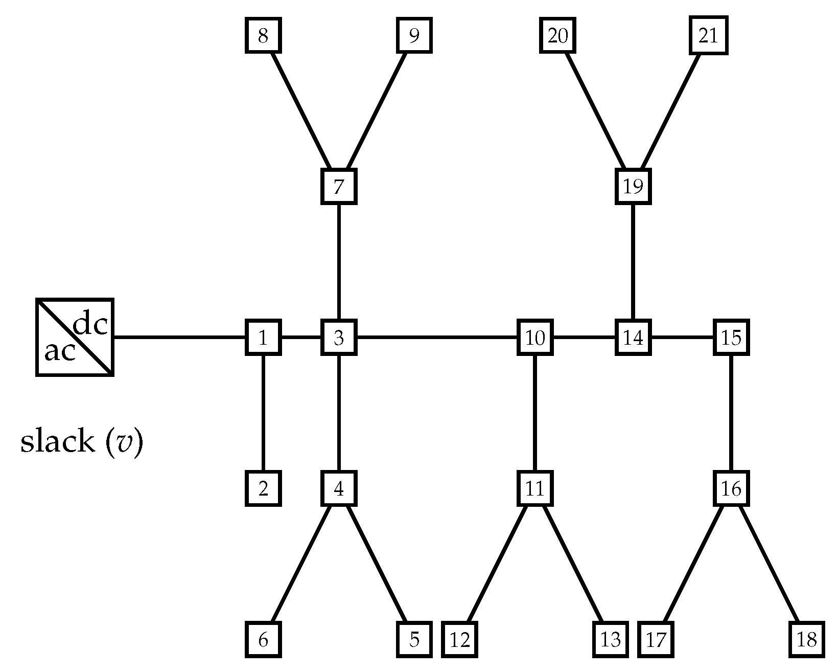
The 21-bus system is an adaptation of the original monopolar DC network proposed by Garces in [20] to demonstrate the convergence of the Newton-Raphson power flow approach in this grid considering drop controllers. The electrical topology of this distribution grid is presented in Figure 2.

The main features assignable to this network are listed below:

i.

The substation bus is located at bus 1, and it operates with a voltage value of $\pm 1$ kV in the positive and negative poles, and it is considered that its neutral pole is solidly grounded.

ii.

The total power consumption in the positive pole is 554 kW, and the total power consumption in the negative pole is 445 kW, while the bipolar load sums 405 kW. This grid has a radial grid configuration.

The complete parametric information for this test feeder is listed in

Table 1. Parametric information regarding the 21-bus grid (all powers in kW).

Node j	Node k	${\mathit{R}}_{\mathbf{jk}}$ ($\mathsf{\Omega }$)	${\mathit{P}}_{\mathit{d},\mathit{k}}^{\mathit{p}}$	${\mathit{P}}_{\mathit{d},\mathit{k}}^{\mathit{n}}$	${\mathit{P}}_{\mathit{d},\mathit{k}}^{\mathit{p}-\mathit{n}}$
1	2	0.053	70	100	0
1	3	0.054	0	0	0
3	4	0.054	36	40	120
4	5	0.063	4	0	0
4	6	0.051	36	0	0
3	7	0.037	0	0	0
7	8	0.079	32	50	0
7	9	0.072	80	0	100
3	10	0.053	0	10	0
10	11	0.038	45	30	0
11	12	0.079	68	70	0
11	13	0.078	10	0	75
10	14	0.083	0	0	0
14	15	0.065	22	30	0
15	16	0.064	23	10	0
16	17	0.074	43	0	60
16	18	0.081	34	60	0
14	19	0.078	9	15	0
19	20	0.084	21	10	50
19	21	0.082	21	20	0

.

To evaluate the efficiency of the proposed recursive quadratic approximation to solve the OPF problem in bipolar DC asymmetric distribution networks is considered that in the 21-bus grid, there are four dispersed generators. The information of these sources is presented in

Table 2. Location and Capacity of the dispersed sources for the 21-bus system.

Node	Location	Capacity (kW)
3	p	300
3	n	100
11	p	400
17	p	200
17	n	300

.

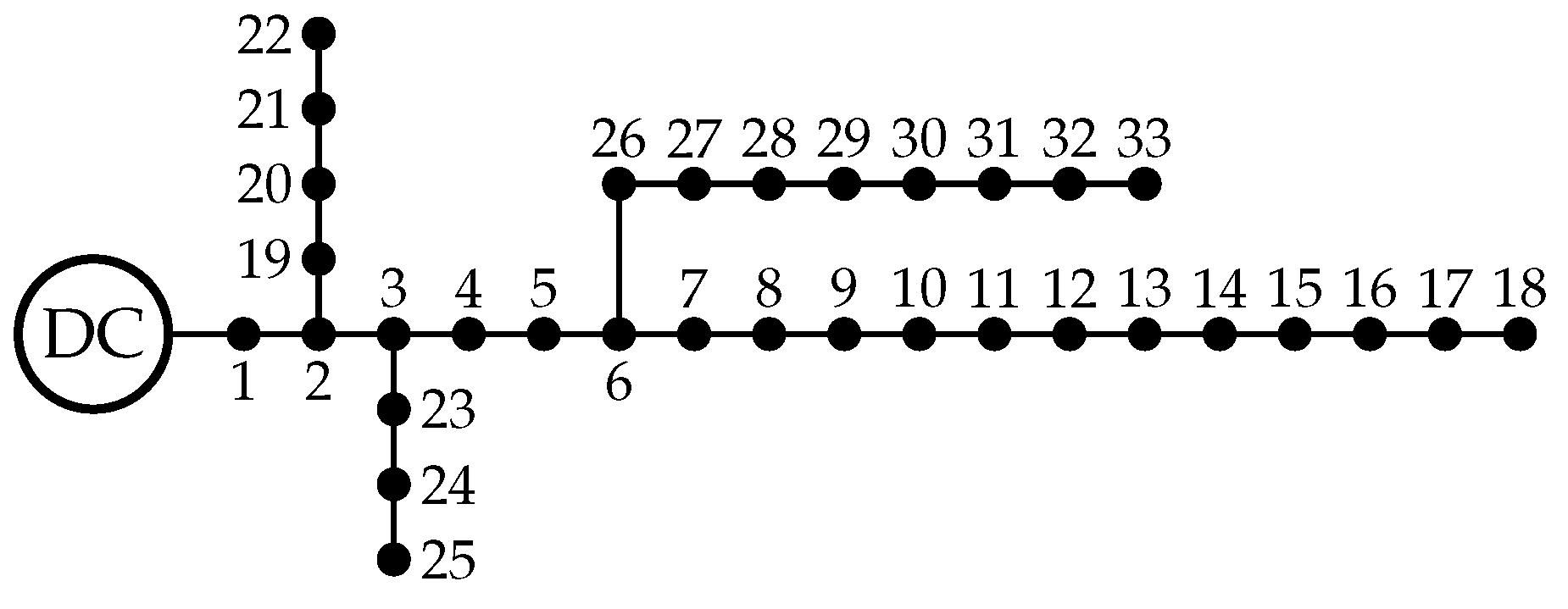
3.6. Bipolar DC 33-Bus System

The 33-bus system is an adaptation of the original IEEE 33-bus grid proposed by authors of [21] to study the problem of the optimal placement and sizing of capacitor banks in radial AC distribution networks. The single-line diagram of this test feeder is presented in Figure 3.

The main characteristics of the bipolar version of the IEEE 33-bus grid are the following:

i.

The substation bus is located at bus 1, and it operates with a voltage value of $\pm 12.66$ kV in the positive and negative poles, and it is considered that its neutral pole is solidly grounded.

ii.

The total power consumption in the positive pole is 2615 kW, and the total power consumption in the negative pole is 2185 kW, while the bipolar loads sum 2350 kW.

Regarding the parametric information of the bipolar DC 33-bus system, all the parameters associated with loads and branches are listed in

Table 3. Parametric information regarding the 33-bus grid (all powers in kW).

Node j	Node k	${\mathit{R}}_{\mathbf{jk}}$ ($\mathsf{\Omega }$)	${\mathit{P}}_{\mathit{d},\mathit{k}}^{\mathit{p}}$	${\mathit{P}}_{\mathit{d},\mathit{k}}^{\mathit{n}}$	${\mathit{P}}_{\mathit{d},\mathit{k}}^{\mathit{p}-\mathit{n}}$
1	2	0.0922	100	150	0
2	3	0.4930	90	75	0
3	4	0.3660	120	100	0
4	5	0.3811	60	90	0
5	6	0.8190	60	0	200
6	7	0.1872	100	50	150
7	8	1.7114	100	0	0
8	9	1.0300	60	70	100
9	10	1.0400	60	80	25
10	11	0.1966	45	0	0
11	12	0.3744	60	90	0
12	13	1.4680	60	60	100
13	14	0.5416	120	100	200
14	15	0.5910	60	30	50
15	16	0.7463	110	0	350
16	17	1.2890	60	90	0
17	18	0.7320	90	45	0
2	19	0.1640	90	150	0
19	20	1.5042	150	50	115
20	21	0.4095	0	90	0
21	22	0.7089	0	90	145
3	23	0.4512	90	110	35
23	24	0.8980	120	0	40
24	25	0.8960	150	100	100
6	26	0.2030	60	80	0
26	27	0.2842	60	0	225
27	28	1.0590	0	0	130
28	29	0.8042	120	75	65
29	30	0.5075	100	100	0
30	31	0.9744	50	150	125
31	32	0.3105	175	100	75
32	33	0.3410	95	60	120

.

For this test feeder, we consider that the distribution company has installed 6 dispersed generators with the information presented in

Table 4. Location and Capacity of the dispersed sources for the 33-bus grid.

Node	Location	Capacity (kW)
10	p	800
12	n	1000
15	p	950
15	n	950
30	p	1350
31	n	1125

.

4. Computational Results

The MATLAB programming environment, version $2021b$, was used on a PC with an AMD Ryzen 7 3700 $2.3$ GHz processor, and 16.0 GB RAM, was used for the computational validation running on a 64-bit version of Microsoft Windows 10 Single Language. The solution of the sequential quadratic programming model (33)–(52) was reached in the convex disciplined tool environment (known as CVX) for MATLAB using the Gurobi solver. In addition, our scripts implemented all the metaheuristic optimizers in the MATLAB programming environment.

4.1. Results for the Bipolar DC 21-Bus System

4.1.1. Power Flow Solution

To demonstrate the effectiveness of the proposed recursive quadratic approximation (RQA) in solving the OPF problem in bipolar asymmetric DC networks. The first comparative analysis considers its comparison of the conventional power flow problem with classical power flow methods. The considered approaches are: (i) the successive approximation power flow (SAPF) method [9], (ii) the triangular-based power flow (TBPF) method [8], and (iii) the hyperbolic approximation power flow (HAPF) method [14].

Table 5. Comparison between power flow methods and the RQA for solidly-ly grounded and neutral floating scenarios in the 21-bus grid.

Neutral wire solidly grounded
Method	Losses (pu)	Iterations	Time (ms)
SAPF	0.954237	13	0.5275
TBPF	0.954237	13	0.8340
HAPF	0.954237	13	1.5542
RQA	0.954237	4	—
Neutral wire floating
Method	Losses (pu)	Iterations	Time (ms)
SAPF	0.912701	10	0.4911
TBPF	0.912701	10	0.7672
HAPF	0.912701	4	1.0212
RQA	0.912701	4	—

presents the comparative results when the proposed RQA is used to solve the power flow problem in bipolar asymmetric DC networks. Note that for all these comparisons, we consider the convergence error as $\epsilon =1\times {10}^{-10}$, which is the maximum difference allowed for voltages in two consecutive iterations.

Numerical results in Table 5 show that:

i.

As expected, all the power flow approaches, including the proposed RQA find the same value for the total grid power loss with a value of $95.4237$ kW for the neutral solidly-ly grounded operation scenario, and $91.2701$ kW in the neutral floating case. In addition, the SAPF and the TBPF take the same number of iterations in both cases, which is an expected result since both methods are from the same family of solution methods, i.e., derivative-free methods from the family of graph-based theory approaches.

ii.

The difference between power losses when considering the neutral wire operating with or without grounded connections is about $4.1536$ kW. This confirms, as expected that the best possible scenario for electrical networks is when the neutral wire is solidly grounded since it minimizes energy losses in this wire while allowing a local voltage reference for each load.

iii.

The HAPF approach showed a notable difference regarding the number of iterations when both simulation scenarios are compared. This is because for the neutral wire to be solidly grounded, it only takes 4 iterations. In contrast, when the neutral wire is floating, it takes 13 iterations, which in the first case it has quadratic convergence, whereas in the second case, it has linear convergence.

Regarding the proposed RQA it is noted that in both simulation scenarios, it takes four4 iterations to find the solution to the power flow problem with the same numerical value in the grid power losses compared with the conventional power flow approaches. This demonstrates that the proposed convex reformulation represents the power balance equations adequately. However, regarding processing times, it is noted that the RCA takes about 6 seconds in both simulation cases. However, in Table 5, all the power flow approach takes a few milliseconds to solve the problem. Nevertheless, it is expected behavior since the RQA addresses the OPF problem as an optimization model which multiple constraints, while the power flow methods (i.e., SAPF, TBPF, and HAPF) use an iterative formula specially developed for the power flow solution.

4.1.2. OPF Solution

Here, we present the effectiveness of the proposed RQA in solving the OPF problem in bipolar asymmetric DC distribution networks with multiple dispersed generators. To compare our proposal, three metaheuristic optimization algorithms are widely known in the current literature to solve nonlinear optimization problems. These algorithms are: The black-hole optimizer (BHO) [22]; (ii) the sine-cosine algorithm (SCA) [23]; and (iii) the vortex-search algorithm (VSA) [24]. For all ofall these metaheuristics, 1000 iterations were assigned, with 10 individuals in their populations and 100 consecutive repetitions for making statistical analyses.

Table 6. Evaluation of the different alternatives to solve the OPF problem in bipolar asymmetric DC networks (all values in pu).

Method	Min.	Mean	Max.	Std. Dev.	Time (s)
SCA	0.23054	0.25305	0.29703	$1.39\times {10}^{-2}$	6.7870
BHO	0.23066	0.23183	0.23329	$5.90\times {10}^{-4}$	13.1513
VSA	0.22986	0.22986	0.22988	$4.23\times {10}^{-6}$	8.3176
SQA	0.22985	0.22985	0.22985	<$1\times {10}^{-16}$	7.7901

presents the comparative results between the RQA and the combinatorial optimization methods. In addition, only the simulation scenario with the neutral wire floating is analyzed since it is the worst case in terms of grid power losses. It is worth mentioning that a master-slave optimization approach was employed for implementing all the metaheuristic optimizers. The master stage was entrusted with defining the optimal values of power injections in generators. However, the slave stage evaluates the amount of grid power losses by using the SAPF approach [25].

Results in Table 6 reveal that:

i.

The proposed RQA finds the best solution to the OPF problem with a value of $22.985$ kW, followed only by a similar value for the VSA. However, the proposed approach has the same numerical solution at each evaluation (convexity of the solution space) with a standard deviation lower than $1\times {10}^{-16}$. However, the VSA approach does not necessarily finds find the same objective function value (see its maximum value). This is an expected behavior for metaheuristics since their random nature makes it impossible to ensure 100% of convergence in nonlinear non-convex optimization problems, as in the case of the exact NLP that represents the studied OPF problem.

ii.

The SCA and the BHO approaches have stuck in locally optimal solutions which are explainable in their random nature and their simple evolution rules (less sophisticated than the VSA approach); however, both can be considered adequate approximations to the OPF solution for problems where high precision is not relevant.

iii.

Regarding processing times in Table 6, the best metaheuristic optimizer (the VSA approach) takes about 8.3176 s to solve the OPF problem, while the worst approach in terms of processing times corresponds to the BHO method with 13.1513 s. Nevertheless, the proposed RQA takes about 7.7901 s, maintaining a similar time when it was used for solving the power flow problem. Additionally, the proposed model has the main advantage that no statistical studies are required to evaluate its efficiency. The convexity of the solution space in this approximation ensures the 100% of solution repeatability. This does not occur in the case of the combinatorial optimization methods.

Finally, the optimal dispatch found with the RQA for the dispersed generators in the 21-bus grid was the following: At node 3 for the positive pole 267.8682 kW and the negative pole 100 kW; at node 11 is 106.2127 kW for the positive pole (note that in this node there is not a dispersed source at the negative pole); and at node 17, these values were 193.5830 kW, and 205.0908 kW, for the positive and negative poles, respectively. It is worth mentioning that the main characteristic of these values is that in unbalanced bipolar DC networks when there are dispersed generators on both poles of the same node, their work also unbalanced. This is expected since the load unbalances require different levels of power injection at each pole to minimize the total grid power losses as much as possible.

4.2. Results for the Bipolar DC 33-Bus System

In this section, we only present the results reached by the RQA to solve the OPF problem in the bipolar DC 33-bus grid for the neutral floating scenario since, as demonstrated for the 21-bus grid, the RQA allows finding the optimal solution.

Table 7. OPF solution for the bipolar DC 33-bus grid.

Case	Power Loss (kW)	Gen. Positive Pole (kW)	Gen. Negative Pole (kW)	Reduction (%)
Ben. case	344.4797	—	—	—
Case 1	215.7037	$\left[\begin{array}{c}\left(10\right)327.4197\\ \left(15\right)457.9217\\ \left(30\right)576.6784\end{array}\right]$	—	37.3828
Case 2	314.6265	—	$\left[\begin{array}{c}\left(12\right)179.3277\\ \left(15\right)151.0976\\ \left(32\right)334.9579\end{array}\right]$	8.6662
Case 3	28.4942	$\left[\begin{array}{c}\left(10\right)555.9692\\ \left(15\right)835.0393\\ \left(30\right)1013.3334\end{array}\right]$	$\left[\begin{array}{c}\left(12\right)500.8079\\ \left(15\right)623.0057\\ \left(32\right)803.9153\end{array}\right]$	91.7283

presents the power flow solution in the benchmark case (without DGs) and the optimal solution of the OPF problem considering three cases: (i) the optimal dispatch of the DGs only for the positive pole; (ii) the optimal dispatch of the DGs only for the negative pole; and (iii) the OPF solution for all the DGs available.

Numerical results in Table 7 reveal that:

i.

The maximum reduction regarding power loss reduction is reached when the DGs in both poles are optimally dispatched. This reduction is higher than 90% concerning the benchmark case. In this scenario, the usage of the DGs capacities was about $77.5594\%$ and $62.6904\%$ in the positive and negative poles, respectively.

ii.

In the case of power dispatch only one pole, the best reduction of power losses is reached in the positive pole, with a value of $37.3828\%$, while for the negative pole, this reduction reaches a value of $8.6662\%$. Two possible facts explain this: (i) the positive pole is the most charged (more power loss when compared with the negative pole), and (ii) the location of the DGs may be better than the DGs in the negative pole.

iii.

Power loss reductions in Table 7 confirm that the OPF problem in bipolar DC networks is indeed a complex optimization problem where the superposition method is not applicable since the model is nonlinear. This is demonstrated by the combination of the generations in the positive and negative poles is different from the solution when all the distributed generators are optimally dispatched.

Regarding processing times for all the simulation cases in Table 7, the proposed RQA took less than 20 s. This processing time confirms the convex theory’s effectiveness and robustness in optimally solving optimization problems without recurring combinatorial methods that cannot ensure global convergence properties.

5. Conclusions and Future Works

A new recursive quadratic approximation to address the OPF problem in bipolar asymmetric DC distribution networks was proposed in this research. The exact NLP model was transformed into a convex approximation by obtaining a linear equivalent formulation of the demanded currents as a function of their voltage magnitudes. This was allowed by approximating the hyperbolic relationship between powers and voltages in these nodes using a linear function. In the case of dispersed generators, the nonlinear relationship between voltage magnitudes and powers was relaxed using their expected operative point by considering that the voltage magnitudes have slight variations compared to the power outputs on these sources.

Numerical simulations in the 21-bus grid considering neutral wire grounded and non-grounded revealed that:

i.

The proposed RQA can efficiently solve the power flow problem in bipolar DC networks by finding the same numerical result in power losses compared with specialized power flow methods as the cases of the SAPF, TBPF, and the HAPF approaches. When the neutral wire is solidly grounded, the total grid power loss was $91.2701$ kW, which increased to $95.4237$ kW in the case of a non-grounded connection.

ii.

Comparative analysis with combinatorial optimizers showed that the proposed RQA efficiently solved the OPF problem in the case of the neutral wire floating. Numerical comparisons with the BHO, the SCA, and the VSA demonstrated that the RQA found the optimal solution with a final value of $22.985$ kW with a standard deviation lower than $1\times {10}^{-16}$. Only the VSA approach found a similar objective function value. However, its standard deviation is about $4.23\times {10}^{-6}$, which means that statistical analysis is required to confirm its effectiveness, which is not the case for the proposed RQA owing to the convex nature of the solution space.

In the case of the bipolar DC 33-bus grid, the nonlinear nature of the OPF problem was confirmed with three different simulation cases. The first case considered the optimal dispatch of the DGs connected only to the positive pole, which permitted a reduction of about $37.3828\%$ of the power loss regarding the benchmark case. The second case considered the optimal dispatch of the DG sources connected only to the negative pole, which only allowed a reduction of about $8.6662\%$. The third case considered the optimal dispatch of all the DGs simultaneously, which permitted a reduction higher than 90% in the total grid power loss.

In future works, it will be possible to make the following contributions: (i) to propose a mixed-integer convex approximation to locate and size dispersed generators in bipolar DC networks and (ii) to extend the proposed RQA to solve the problem of the optimal pole-swapping problem in bipolar asymmetric distribution networks.

References

- Chaves, M.; Margato, E.; Silva, J.F.; Pinto, S.F.; Santana, J. HVDC transmission systems: Bipolar back-to-back diode clamped multilevel converter with fast optimum-predictive control and capacitor balancing strategy. Electr. Power Syst. Res. 2011, 81, 1436–1445. [Google Scholar] [CrossRef]
- Li, Z.; Zhan, R.; Li, Y.; He, Y.; Hou, J.; Zhao, X.; Zhang, X.P. Recent developments in HVDC transmission systems to support renewable energy integration. Glob. Energy Interconnect. 2018, 1, 595–607. [Google Scholar] [CrossRef]
- Rivera, S.; Lizana, R.; Kouro, S.; Dragicevic, T.; Wu, B. Bipolar DC Power Conversion: State-of-the-Art and Emerging Technologies. IEEE J. Emerg. Sel. Top. Power Electron. 2021, 9, 1192–1204. [Google Scholar] [CrossRef]
- Yang, M.; Zhang, R.; Zhou, N.; Wang, Q. Unbalanced voltage control of bipolar DC microgrid based on distributed cooperative control. In Proceedings of the 2020 15th IEEE Conference on Industrial Electronics and Applications (ICIEA), Kristiansand, Norway, 9–13 November 2020. [Google Scholar] [CrossRef]
- Guo, C.; Wang, Y.; Liao, J. Coordinated Control of Voltage Balancers for the Regulation of Unbalanced Voltage in a Multi-Node Bipolar DC Distribution Network. Electronics 2022, 11, 166. [Google Scholar] [CrossRef]
- Chew, B.S.H.; Xu, Y.; Wu, Q. Voltage Balancing for Bipolar DC Distribution Grids: A Power Flow Based Binary Integer Multi-Objective Optimization Approach. IEEE Trans. Power Syst. 2019, 34, 28–39. [Google Scholar] [CrossRef] [Green Version]
- Montoya, O.D.; Medina-Quesada, Á.; Hernández, J.C. Optimal Pole-Swapping in Bipolar DC Networks Using Discrete Metaheuristic Optimizers. Electronics 2022, 11, 2034. [Google Scholar] [CrossRef]
- Medina-Quesada, Á.; Montoya, O.D.; Hernández, J.C. Derivative-Free Power Flow Solution for Bipolar DC Networks with Multiple Constant Power Terminals. Sensors 2022, 22, 2914. [Google Scholar] [CrossRef]
- Montoya, O.D.; Gil-González, W.; Garcés, A. A successive approximations method for power flow analysis in bipolar DC networks with asymmetric constant power terminals. Electr. Power Syst. Res. 2022, 211, 108264. [Google Scholar] [CrossRef]
- Lee, J.O.; Kim, Y.S.; Jeon, J.H. Optimal power flow for bipolar DC microgrids. Int. J. Electr. Power Energy Syst. 2022, 142, 108375. [Google Scholar] [CrossRef]
- Garces, A.; Montoya, O.D.; Gil-Gonzalez, W. Power Flow in Bipolar DC Distribution Networks Considering Current Limits. IEEE Trans. Power Syst. 2022, 37, 4098–4101. [Google Scholar] [CrossRef]
- Marini, A.; Mortazavi, S.; Piegari, L.; Ghazizadeh, M.S. An efficient graph-based power flow algorithm for electrical distribution systems with a comprehensive modeling of distributed generations. Electr. Power Syst. Res. 2019, 170, 229–243. [Google Scholar] [CrossRef]
- Shen, T.; Li, Y.; Xiang, J. A Graph-Based Power Flow Method for Balanced Distribution Systems. Energies 2018, 11, 511. [Google Scholar] [CrossRef] [Green Version]
- Sepúlveda-García, S.; Montoya, O.D.; Garcés, A. Power Flow Solution in Bipolar DC Networks Considering a Neutral Wire and Unbalanced Loads: A Hyperbolic Approximation. Algorithms 2022, 15, 341. [Google Scholar] [CrossRef]
- Mackay, L.; Dimou, A.; Guarnotta, R.; Morales-Espania, G.; Ramirez-Elizondo, L.; Bauer, P. Optimal power flow in bipolar DC distribution grids with asymmetric loading. In Proceedings of the 2016 IEEE International Energy Conference (ENERGYCON), Leuven, Belgium, 4–8 April 2016; pp. 1–6. [Google Scholar]
- Mackay, L.; Guarnotta, R.; Dimou, A.; Morales-Espana, G.; Ramirez-Elizondo, L.; Bauer, P. Optimal power flow for unbalanced bipolar DC distribution grids. IEEE Access 2018, 6, 5199–5207. [Google Scholar] [CrossRef]
- Lee, J.O.; Kim, Y.S.; Moon, S.I. Current injection power flow analysis and optimal generation dispatch for bipolar DC microgrids. IEEE Trans. Smart Grid 2020, 12, 1918–1928. [Google Scholar] [CrossRef]
- Jat, C.K.; Dave, J.; Van Hertem, D.; Ergun, H. Unbalanced OPF Modelling for Mixed Monopolar and Bipolar HVDC Grid Configurations. arXiv 2022, arXiv:2211.06283. [Google Scholar]
- Montoya, O.D.; Zishan, F.; Giral-Ramírez, D.A. Recursive Convex Model for Optimal Power Flow Solution in Monopolar DC Networks. Mathematics 2022, 10, 3649. [Google Scholar] [CrossRef]
- Garces, A. On the Convergence of Newton’s Method in Power Flow Studies for DC Microgrids. IEEE Trans. Power Syst. 2018, 33, 5770–5777. [Google Scholar] [CrossRef] [Green Version]
- Baran, M.; Wu, F. Optimal sizing of capacitors placed on a radial distribution system. IEEE Trans. Power Deliv. 1989, 4, 735–743. [Google Scholar] [CrossRef]
- Kumar, S.; Datta, D.; Singh, S.K. Black Hole Algorithm and Its Applications. In Studies in Computational Intelligence; Springer International Publishing: Berlin/Heidelberg, Germany, 2014; pp. 147–170. [Google Scholar] [CrossRef]
- Gabis, A.B.; Meraihi, Y.; Mirjalili, S.; Ramdane-Cherif, A. A comprehensive survey of sine cosine algorithm: Variants and applications. Artif. Intell. Rev. 2021, 54, 5469–5540. [Google Scholar] [CrossRef]
- Doğan, B.; Ölmez, T. Vortex search algorithm for the analog active filter component selection problem. AEU-Int. J. Electron. Commun. 2015, 69, 1243–1253. [Google Scholar] [CrossRef]
- Grisales-Noreña, L.; Montoya, D.G.; Ramos-Paja, C. Optimal Sizing and Location of Distributed Generators Based on PBIL and PSO Techniques. Energies 2018, 11, 1018. [Google Scholar] [CrossRef]
Figure 2.
Single-diagram of the 21-bus grid.
Figure 3.
Adaptation of the IEEE 33-bus grid for DC bipolar applications.