Ocean Wave Energy Control Using Aquila Optimization Technique

Abstract

This paper presents ocean wave energy control using the Aquila optimization (AO) technique. An oscillating water column (OWC)-type wave energy converter has been considered that is fitted with a Wells turbine and doubly fed induction generator (DFIG). To achieve maximum power point tracking (MPPT), the rotor speed of the DFIG must be controlled as per the MPPT law. The MPPT law is designed in such a way that the Wells turbine flow coefficient remains within the threshold limit. It avoids the turbine from stalling which generates the maximum power. The MPPT law provides the reference rotor speed which is followed by the actual rotor speed. For this, a backstepping controller (BSC)-based rotational speed control strategy has been designed using the Lyapunov stability theory. The BSC has unknown control parameters which should be selected such that tracking errors are minimum. Hence, the objective of this work is to find the unknown control parameters using an optimization approach. The optimization approach of selecting BSC control parameters for an OWC plant has not been explored yet. To achieve this, an integral square error (ISE)-type fitness function has been defined and minimized using the AO technique. The results achieved using the AO technique have been compared with particle swarm optimization (PSO) and a genetic algorithm (GA), validating its superior performance. The rotor speed error maximum peak overshoot is least for AO-BSC as compared to PSO-BSC and GA-BSC. The fitness function value for AO comes out to be least among all the optimization methods applied. However, all tested methods provide satisfactory results in terms of turbine flow coefficient, rotor speed and output power. The approach paves the way for future research on ocean wave energy control.

1. Introduction

Renewable energy research is gaining popularity due to the increasing concerns over depleting natural resources and greenhouse emissions. There are several forms of renewable energy such as solar [1], wind [2], tidal [3], hydro [4], ocean wave [5,6], etc. Solar energy is a renewable energy source that can be used indefinitely without depleting natural resources but the amount of energy that solar panels can generate is dependent on the weather and can vary from day to day or season to season. Like solar energy, wind energy is a renewable energy source that does not deplete natural resources. However, the amount of energy that wind turbines can generate is dependent on the weather. Similarly, tidal energy can only be harnessed in locations with significant tidal ranges, which limits its availability as a power source. Ocean wave energy is an excellent source of renewable energy that can be tapped into by the proper design of energy converters and their controllers. Furthermore, ocean waves are present year-round, persisting both during the daytime and nighttime. An oscillating water column (OWC) is a technology used to convert the energy of ocean waves into electricity [7]. An OWC system consists of a chamber that is open to the ocean, and as waves enter the chamber, they compress the air inside, which drives a turbine to generate electricity. The torque coefficient and flow behavior of the turbine plays a key role in converting mechanical energy into electrical energy efficiently [8]. To ensure the efficiency and stability of an OWC system, it is necessary to have a control system that monitors and adjusts the system’s performance.

The control of an OWC system involves several key aspects. One of the most important is the control of the air pressure inside the chamber. The pressure inside the chamber needs to be maintained at a certain level to ensure that the turbine is operating at the optimal speed. The control system can adjust the air pressure by controlling the amount of air that is allowed to enter or leave the chamber. Another important aspect of the control of an OWC system is the control of the turbine’s speed. The speed of the turbine needs to be adjusted to match the frequency of the incoming waves to ensure that the maximum amount of energy is extracted from the waves. The control system can adjust the speed of the turbine by adjusting the pitch of the turbine blades or by adjusting the amount of torque applied to the generator. The control of an OWC system is critical to ensure that the system is operating efficiently and generating electricity at its maximum potential. The control system needs to monitor and adjust the air pressure, turbine speed and other operating parameters to ensure that the system is operating within its optimal range. Nonlinear control strategies have gained popularity due to their ability to handle the complex dynamics of the OWC system. In this literature review, we will examine some of the recent developments in the nonlinear rotational speed control of OWCs.

A comprehensive review of wave power system controllers, including those for oscillating water column (OWC) devices, was conducted in [9]. The integration of local grid storage with OWC systems was proposed in [10], while [11] employed a rotor speed optimization technique for achieving maximum power point tracking (MPPT) in OWCs. An innovative latching control strategy for MPPT in floating OWC wave power converters was presented in [12]. In [13], a peak-power control scheme was developed for grid-connected OWCs, and its effectiveness was validated through large-scale testing. A fuzzy-backstepping-based speed controller was developed in [14], and three Lyapunov-based nonlinear controllers were introduced in [15] for regulating the DC link voltage, rotor speed and grid-side converter of the doubly fed induction generators (DFIGs) employed in OWCs. Regarding Wells turbines, a flow controller was devised in [16] to optimize the extraction of wave power. An event-triggered controller for OWC energy plants was described in [17] with a focus on reducing the frequency of control updates between the controller and plant. The authors of [18] presented an enhanced variant of the conventional airflow controller, employing fuzzy gain scheduling and a PI-type controller for OWCs. Several AI-based airflow controller approaches have been proposed recently [19,20,21]. The harmony search algorithm was employed in four different implementations to optimize the proportional–integral–derivative (PID) controller within the airflow control system [19]. Another method for airflow control, based on breaking symmetry, was introduced in [20]. Furthermore, an artificial neural network-based airflow controller utilizing surface elevation measurements was developed [21], considering the power generated by the NEREIDA wave power plant and actual wave input data. For additional insights into OWC plant control, refer to [22]. In [23], a comprehensive analysis of the dynamics and control of air turbines and electrical generators in OWCs was conducted using data from the Mutriku wave power plant. The study compared Wells turbines with bi-radial turbines, demonstrating the superiority of the bi-radial turbine design over the Wells turbine configuration.

In reference [24], a centralized airflow management technique is presented for a complex ocean energy system with the aim of reducing output power variance. The paper in [25] provides a straightforward methodology for developing a PID controller that effectively manages the turbine velocity of an ocean wave converter (OWC) system. The primary objective of the PID controller is to optimize the extraction of wave energy from the OWC system. In [26], a unique approach called a fuzzy gain scheduled-sliding mode controller (FGS-SMC) is employed to simulate an OWC system and achieve the precise control of the rotating velocity, ensuring stable operation without stalling. The effectiveness of the FGS-SMC technique in enhancing the operational efficiency of the OWC system is demonstrated. Additionally, [27] introduces a fuzzy logic controller (FLC) and an airflow reference generator, which are designed and validated in a simulation environment to showcase how the precise control of the turbine speed can increase the overall efficiency of an OWC system. These control mechanisms offer promising avenues for optimizing the performance of OWC systems. In [28], a nonlinear model predictive controller (NMPC) is developed to maintain the efficacy of a self-rectifying turbine coupled with an OWC system, while simultaneously maximizing the generation of electro-mechanical power. The NMPC approach proves to be effective in controlling the OWC system and maximizing power generation. Moreover, [29] presents a state-space modeling approach to capture the array of OWC wave energy converters (WECs) and address their nonlinear dynamics. To maintain a reference turbine angular speed and generate a smooth torque signal for the generator, a second-order sliding mode controller (SMC) is designed. This control mechanism enhances the stability and performance of the OWC system. The control strategies for a small-scale WEC utilizing a permanent magnet synchronous generator (PMSG) are investigated in [30]. The paper assesses the effectiveness of two control strategies, namely robust adaptive control (RAC) and conventional field-oriented control (FOC), in optimizing the performance of the WEC. In [31], the modeling and control of OWC was presented where linear and nonlinear controllers were described. In [32], many control techniques were reviewed for wave energy converters. In the study presented in [33], deep learning techniques were employed to predict the rotational speed of the turbine generator in an oscillating water column wave energy converter (OWC-WEC).

Reference [34] presents a comprehensive wave-to-wire model specifically designed to assess the energy conversion process from wave resources to the electrical grid in wave energy converters (WECs) based on the oscillating water column (OWC) principle. The model offers an integrated solution that encompasses the primary converter (chamber), the secondary converter (air turbine) and the tertiary converter (electric generator). This holistic approach allows for a thorough evaluation of the entire energy conversion chain, providing valuable insights into the performance and efficiency of OWC-based WEC systems. In [35], the operation of a Wells turbine for OWC systems was analyzed with an analytical model and computational fluid dynamics models. Analytical and numerical models were applied to determine the operating curves of a laboratory-scale turbine. In [36], an intelligent control algorithm was proposed to enhance the robustness of the permanent magnet synchronous generator (PMSG)-based oscillating water column (OWC) system. This algorithm generates precise signals to the PMSG, enabling better control of the power system and achieving a superior dynamic response compared to other intelligent control algorithms. The study presented in [37] highlights that the existing power conversion technology for wave energy converters (WECs) is still influenced by wind systems, indicating the need for further optimization to meet the specific requirements of WECs. In [38], an inverse model for the OWC system at the Mutriku power plant was derived using fuzzy modeling and optimized through genetic algorithms. The proposed strategy demonstrated significant annual improvements, with an average increase of over 9% in generator power. A novel peak shaving control strategy was introduced in [39] to reduce the energy costs of OWC-based WECs. This algorithm was tested in real sea conditions at the Mutriku wave power plant, showcasing its effectiveness in optimizing energy generation and consumption.

Nonlinear control strategies have shown promise in improving the performance of OWC wave energy converters by regulating the rotational speed of the turbine. The studies reviewed in this literature review demonstrate the effectiveness of different nonlinear control methods. Further research is needed to explore the applicability of these methods in practical OWC systems and to optimize their performance.

The Aquila optimization technique is a relatively new meta-heuristic optimization algorithm that is inspired by the hunting behavior of the eagle. This optimization technique was proposed in 2019 and has been used to solve various optimization problems in engineering, economics and other fields [40]. One of the main advantages of Aquila optimization is its ability to find the global optimum of a given problem with high accuracy and efficiency. This is because the algorithm uses a combination of exploration and exploitation strategies, which allows it to effectively search the solution space for the best possible solution. Another advantage of Aquila optimization is its simplicity and ease of implementation. The algorithm only requires a few parameters to be set, and it does not require any special mathematical or computational skills to use.

In this paper, the backstepping control (BSC) has been designed to control the rotational speed of the OWC plant. The BSC algorithm has some tunable parameters which should be chosen optimally to achieve the best possible outcome from the controller. Although BSC was designed in [14,17,24], the BSC parameters were chosen manually using a trial-and-error approach. To choose the BSC parameters optimally, there is need to define a fitness function depending on the error function of the controller. This fitness function must be minimized using a suitable optimization algorithm. One of the recent algorithms is the Aquila optimizer (AO) which has a better performance than already-established optimization techniques. The proposed work has the following novel contributions:

• This study proposes the optimization approach for tuning the BSC control parameters to achieve the optimum control of an OWC plant. In recent past studies, there was manual tuning of the BSC control parameters which might lead to the poor performance of an OWC plant.
• An integral square error (ISE)-type fitness function has been defined. The AO technique has been applied to minimize the ISE and to obtain the optimized BSC control parameters. This approach has not been applied yet on an OWC plant.
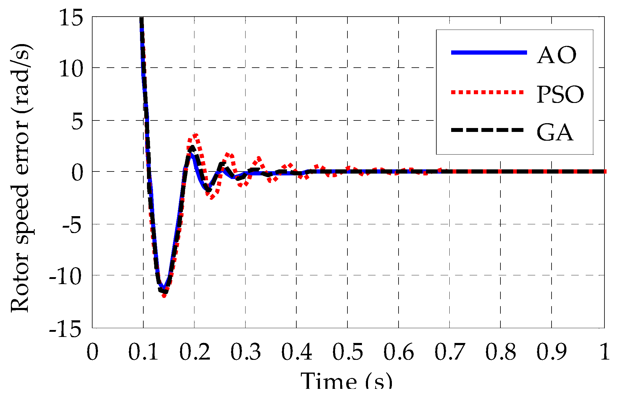
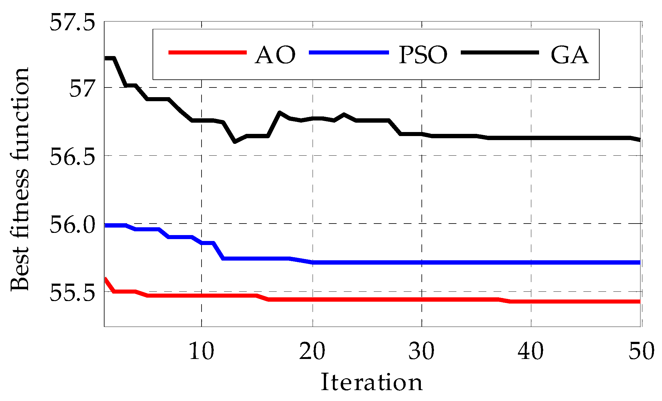
• Additionally, the particle swarm optimization (PSO) and genetic algorithm (GA) technique are also applied which are widely used optimizers. The details about PSO and GA can be found in [41,42,43,44]. The AO has been compared with the PSO and GA techniques in terms of rotor speed error and fitness function.

The remaining portion of the paper has the following: Section 2 gives an overview of the OWC ocean wave energy plant. In Section 3, the MPPT algorithm and BSC scheme has been designed. In addition, the optimization problem is stated. In Section 4, the AO technique has been discussed. Section 5 discusses the simulation results followed by the conclusion in Section 6.

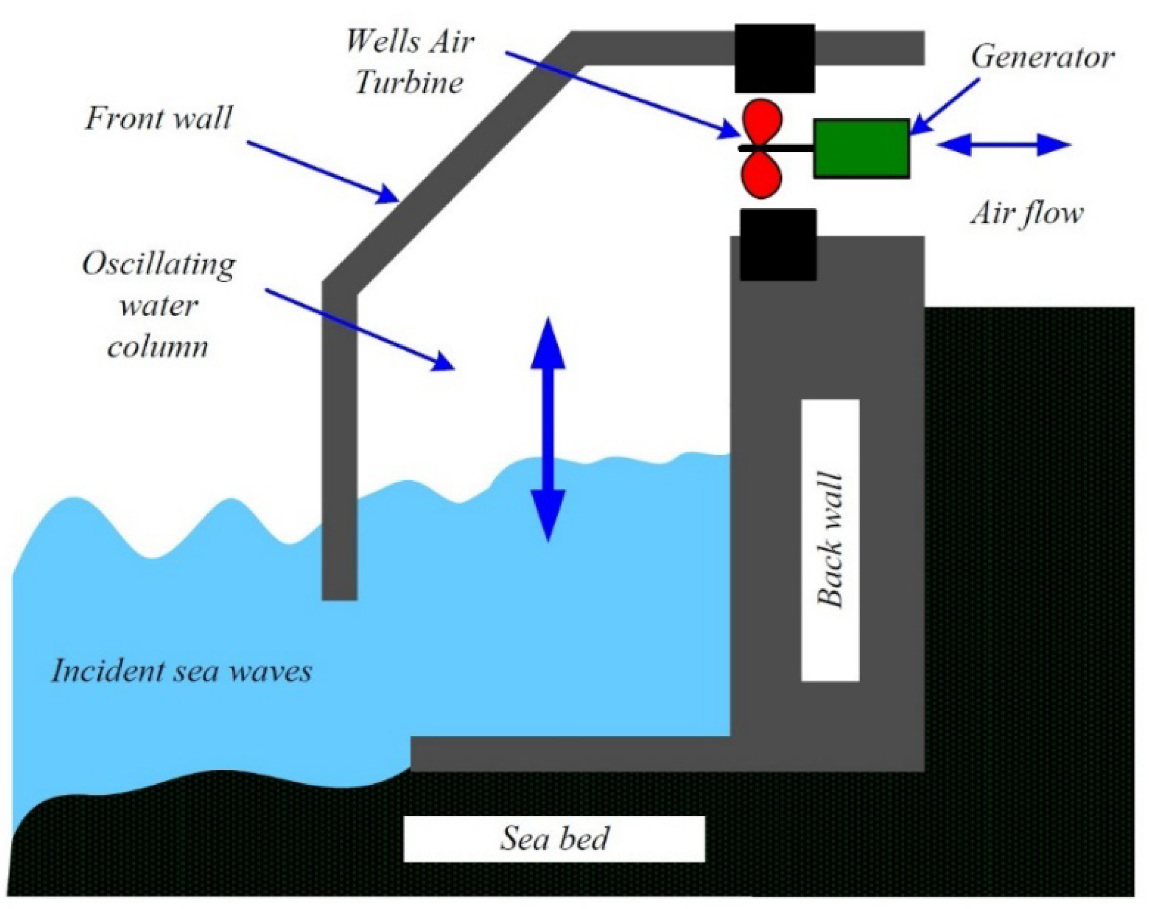
2. Description of OWC and Control Problem Statement

The OWC consists of a partially submerged chamber that is open to the ocean (Figure 1). As waves pass by, the water level in the chamber rises and falls, causing air to be forced in and out of the chamber through a small opening. The moving air drives a turbine, which generates electricity. The motion of the OWC is typically controlled using a control system that adjusts the opening size to maintain the desired air pressure and maximize the energy conversion efficiency.

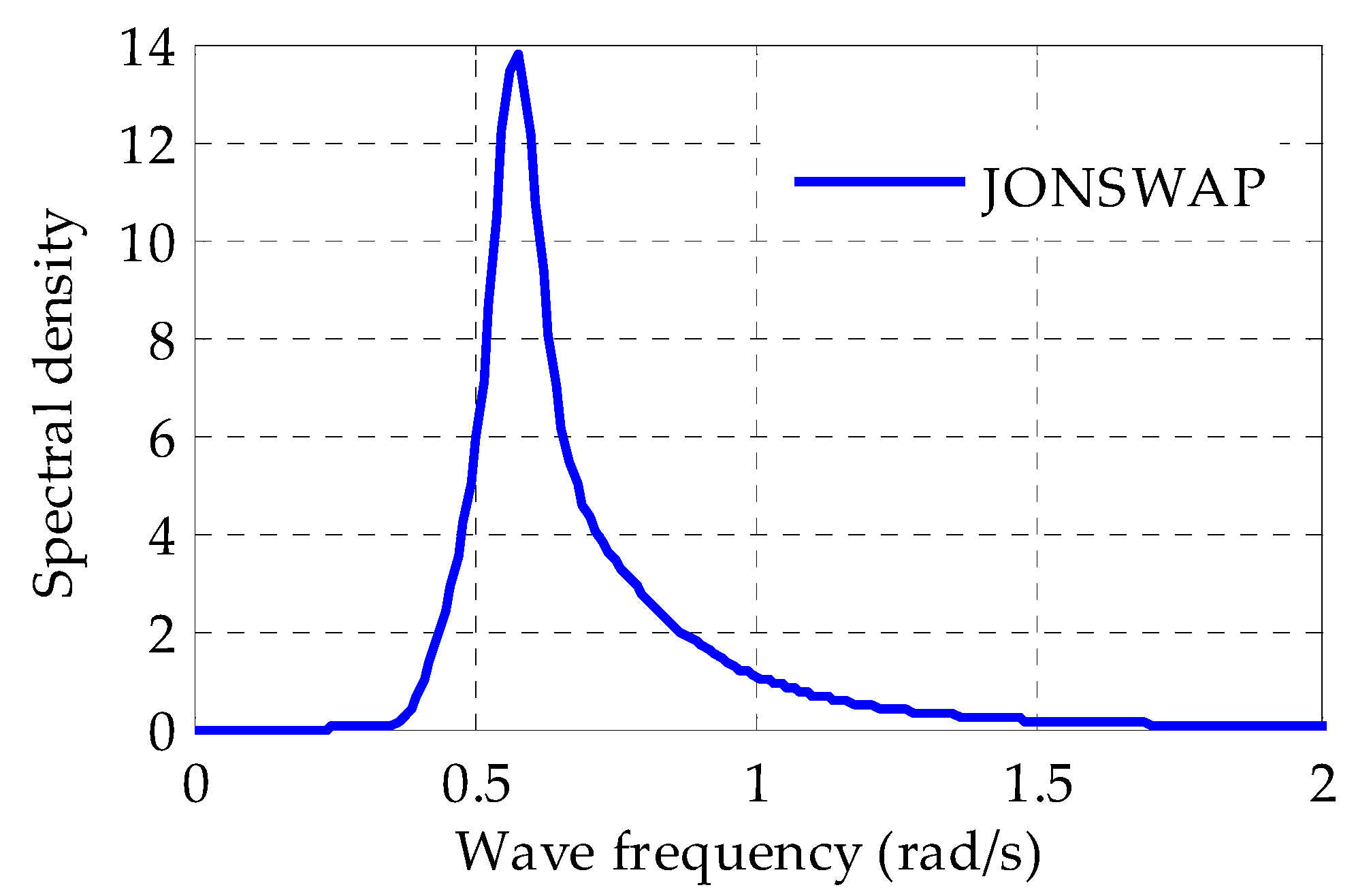
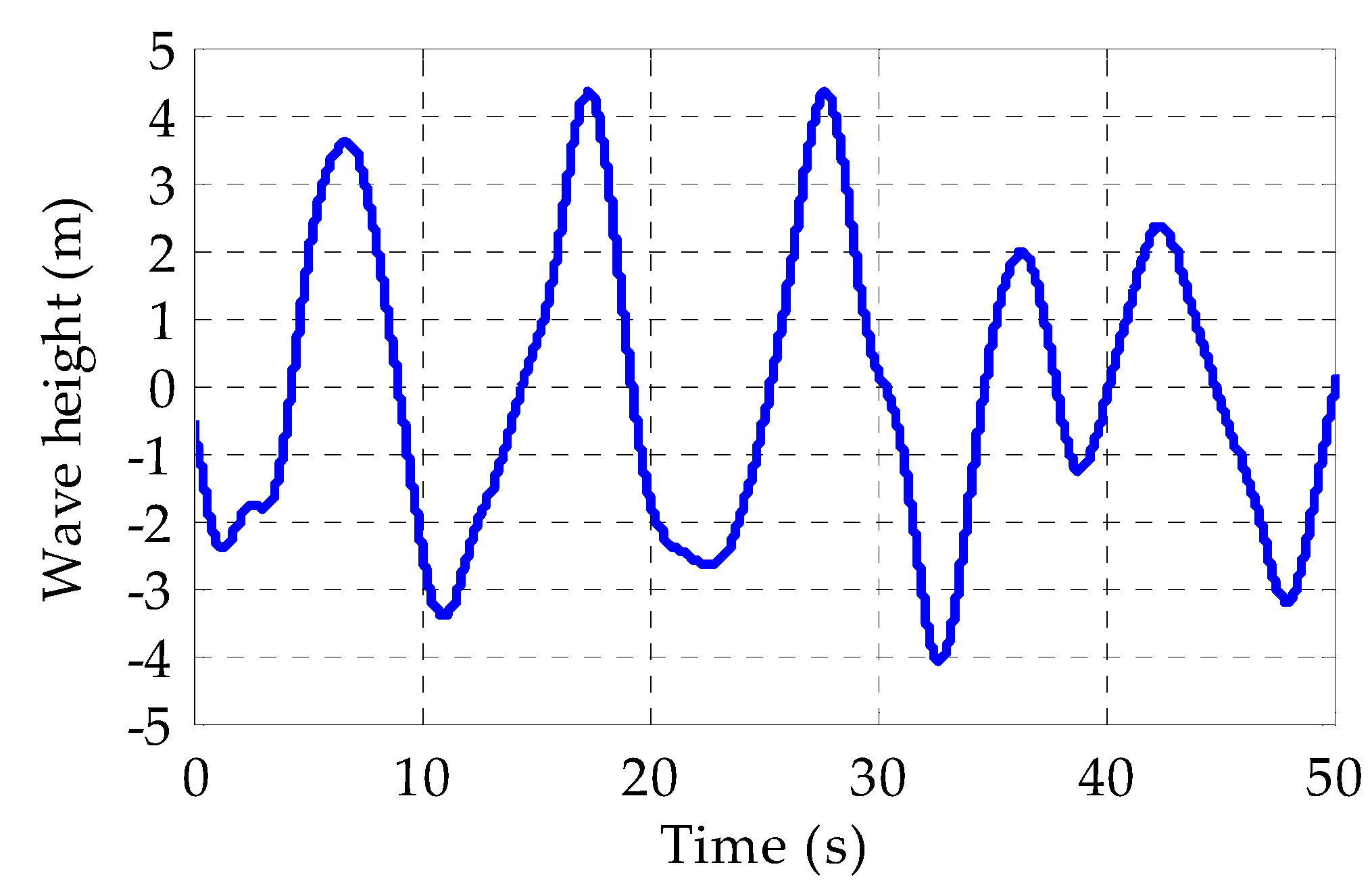
2.1. Wave Modeling and Chamber Dynamics

The JONSWAP model is a well-established theoretical model utilized for the prediction of ocean wave characteristics, taking into account parameters such as wind speed, direction and duration. Developed collaboratively by a group of researchers from multiple European countries in the 1970s, its primary objective was to enhance offshore engineering designs by providing accurate wave predictions. In this study, the effectiveness of the proposed control systems was assessed using the JONSWAP model, a widely accepted simulation tool in wave research. Figure 2 showcases the JONSWAP wave band, exhibiting a prominent frequency peak of approximately 0.5 rad/s.

The OWC comprises a hermetically sealed chamber featuring top and bottom apertures, along with four surrounding side walls (refer to Figure 1). Positioned in the water, the bottom of the chamber is partially submerged and experiences the impact of incoming waves. The variation in sea level, manifested as the wave height, induces a bidirectional airflow within the chamber. The mathematical representation of the air velocity is defined by the equation provided in [24].

$$V_{air}=\left(\frac{A_o}{A_d}\right).\frac{\partial h_w\left(t\right)}{\partial t}$$

(1)

where $A_o$ is the cross-section area of the OWC $\left({\mathrm{m}}^2\right)$, $A_d$ is the cross-section area of turbine duct $\left({\mathrm{m}}^2\right)$, $h_w\left(t\right)$ is the wave height $(\mathrm{m}$) and $V_{air}$ is air velocity $\left(\mathrm{m}/\mathrm{s}\right)$. The representation for air velocity as presented in (1), provides the input to the Wells turbine.

2.2. Wells Turbine Dynamics

Self-rectifying turbines, such as the Wells turbine, are employed in wave energy conversion systems. These turbines facilitate bidirectional airflow while maintaining a consistent rotational direction. However, one of the drawbacks associated with Wells turbines is their susceptibility to stalling behavior, which can adversely impact their performance. The torque of the turbine, $T_{tur}$, is presented as [24]:

$$T_{tur}=f\left({\varphi }_{tur}\right)·V_{air}^2$$

(2)

where $f\left({\varphi }_{tur}\right)$, a function of turbine flow coefficient, ${\varphi }_{tur}$, can be stated as:

$$f\left({\varphi }_{tur}\right)=C_{tur}·k_{tur}·r·\left(1+{\varphi }_{tur}^{-1}\right)$$

(3)

$C_{tur}$ characterizes the Wells turbine characteristics. $C_{tur}$ varies with ${\varphi }_{tur}$ as shown in Figure 3. The turbine flow coefficient, ${\varphi }_{tur}$, is provided by:

$${\varphi }_{tur}=V_{air}·{\left(r{\omega }_{rot}\right)}^{-1}$$

(4)

As demonstrated in Figure 3, ${\varphi }_{tur} \le {\varphi }_{th}=0.3$ offers the highest torque coefficient, which would therefore deliver the most turbine torque and hence the greatest production power. If flow coefficient remains below the threshold value, i.e., ${\varphi }_{tur} \le {\varphi }_{th}=0.3$, turbine torque increases and subsequently the output power increases. However, when ${\varphi }_{tur}>{\varphi }_{th}=0.3$, the turbine torque decreases and thus, the output power starts decreasing.

The Wells turbine is connected to a doubly fed induction generator (DFIG). Consequently, the equation governing the turbo–generator relationship can be expressed as follows:

$$\frac{d{\omega }_{rot}}{dt}=\frac{1}{J}\left(T_{tur}-F·{\omega }_{rot}-T_{gen}\right)$$

(5)

where ${\omega }_{rot}$ is rotor speed; F is frictional coefficient; and $T_{gen}$ is the electro-magnetic torque of DFIG.

2.3. DFIG Dynamics

In this study, a dynamic version of the doubly fed induction generator (DFIG) employing a direct–quadrature (dq) reference frame was considered. The utilization of the dq model offers the advantage of representing all three phases as direct current (dc) quantities within a stationary reference frame using a synchronous rotating frame [24]. The state equations governing the behavior of the DFIG are presented as follows:

$$\frac{d{\lambda }_{ds}}{dt}=-\frac{R_s{L}_r}{Q}{\lambda }_{ds}+{\omega }_e{\lambda }_{qs}+\frac{R_s{L}_m}{Q}{\lambda }_{dr}+v_{ds}$$

(6)

$$\frac{d{\lambda }_{qs}}{dt}=-{\omega }_e{\lambda }_{ds}-\frac{R_s{L}_r}{Q}{\lambda }_{qs}+\frac{R_s{L}_m}{Q}{\lambda }_{qr}+v_{qs}$$

(7)

$$\frac{d{\lambda }_{dr}}{dt}=\frac{R_r{L}_m}{Q}{\lambda }_{ds}-\frac{R_r{L}_s}{Q}{\lambda }_{dr}-({\omega }_{rot}-{\omega }_e){\lambda }_{qr}+v_{dr}$$

(8)

$$\frac{d{\lambda }_{qr}}{dt}=\frac{R_r{L}_m}{Q}{\lambda }_{qs}+({\omega }_{rot}-{\omega }_e){\lambda }_{dr}+v_{qr}$$

(9)

where $Q=L_s{L}_r-L_m^2$. ${\lambda }_{ds}$, ${\lambda }_{qs}$, ${\lambda }_{dr}$ and ${\lambda }_{qr}$ are dq flux quantities. $R_s$ and $R_r$ are DFIG resistances whereas $L_s$, $L_r$ and $L_m$ are DFIG inductances. ${\omega }_e$ is the stator supply frequency, $v_{ds}$, $v_{qs}$, $v_{dr}$ and $v_{qr}$ are DFIG voltages. The flux states ${\lambda }_{ds}$, ${\lambda }_{qs}$, ${\lambda }_{dr}$ and ${\lambda }_{qr}$ have initial conditions ${\lambda }_{ds0}$, ${\lambda }_{qs0}$, ${\lambda }_{dr0}$ and ${\lambda }_{qr0}$, respectively. The electromagnetic torque and output power expressions are:

$$T_{gen}=-M\left({\lambda }_{qs}{\lambda }_{dr}-{\lambda }_{ds}{\lambda }_{qr}\right)$$

(10)

$$P_{gen}=T_{gen}{\omega }_{rot}$$

(11)

where $M=-\left(\frac{3}{2}\right)\left(\frac{p}{2}\right)\left(\frac{L_m}{Q}\right)$. $p$ is the number of poles of DFIG.

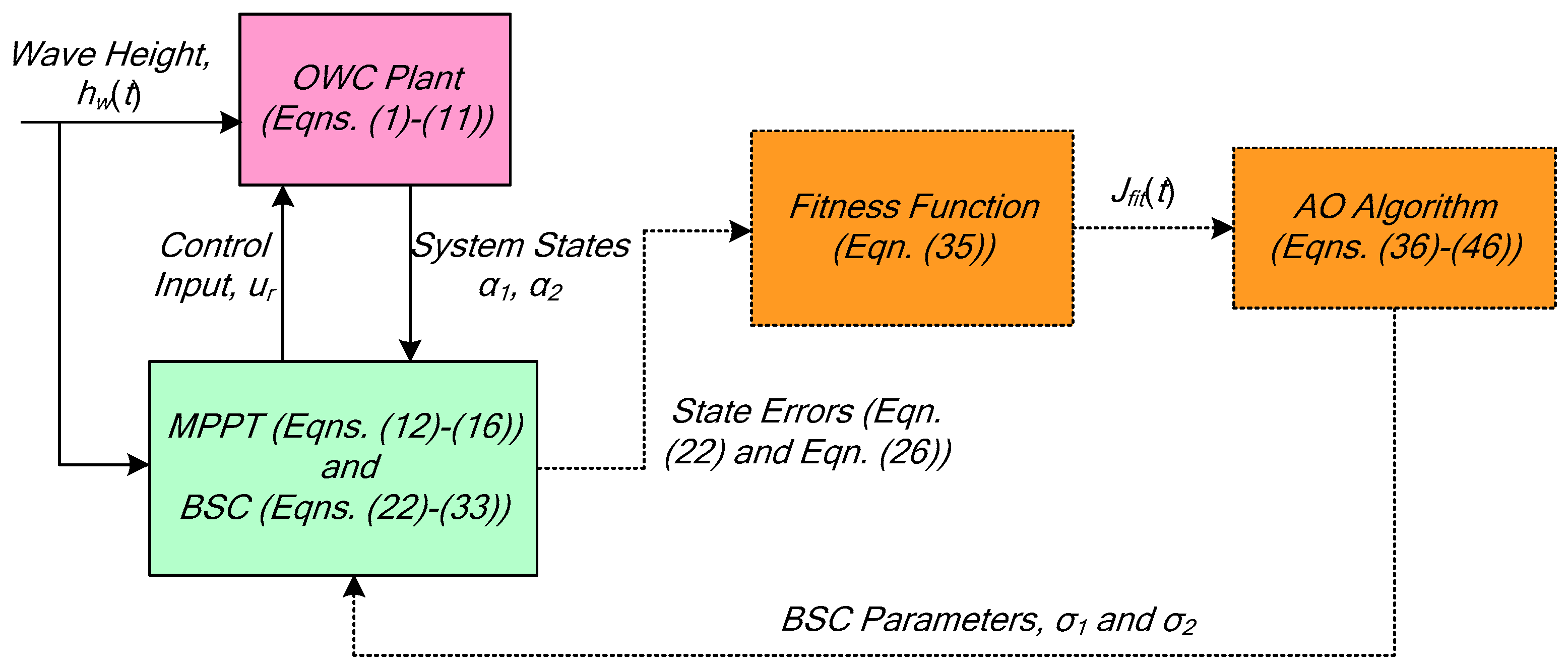
3. Design of BSC Scheme and MPPT Algorithm

3.1. Design of MPPT Scheme

The MPPT algorithm [17] for obtaining the rotor speed reference, ${\alpha }_{1d}$, is presented next. It is evaluated using $V_{air}$ as the following:

Step 1: Evaluate $V_{air}$ from Equation (1).

Step 2: Evaluate the highest values of $V_{air}$ from the procedure given below:

$$\begin{array}{c}if V_{air}\ne 0 and {\dot{V}}_{air}=0 \\ V_{air-p}=V_{air}\\ else \\ V_{air-p}=0\\ end \end{array}\}$$

(12)

Step 3: Obtain the zero-order hold (ZOH) of $V_{air-p}$ as:

$${\overline{V}}_{air-p}=ZOH \left(V_{air-p}\right)$$

(13)

Step 4: For ${\varphi }_{th}=0.3$, evaluate the ${\omega }_{ref}$ using Equation (4) as:

$${\omega }_{ref}={\overline{V}}_{air-p} {\left(r{\varphi }_{th}\right)}^{-1}$$

(14)

Step 5: Limit ${\omega }_{ref}$ to a minimum and maximum level and obtain ${\omega }_{1d}$ as:

$$\begin{array}{c}if {\omega }_{ref}\le {\omega }_e \\ {\omega }_{1d}={\omega }_e \\ else if {\omega }_{ref}\ge {\omega }_e \\ {\omega }_{1d}={\omega }_{rp} \\ else \\ {\omega }_{1d}={\omega }_{ref}\\ end \end{array}\}$$

(15)

where ${\omega }_e<{\omega }_{1d}<{\omega }_{rp}$.

Step 6: To mitigate sudden changes ${\omega }_{1d}$, a low pass filter with impulse response $h_f$ is used as:

$${\alpha }_{1d}=h_f \otimes {\omega }_{1d }$$

(16)

The Laplace representation of $h_f$ is as follows:

$$H_f\left(s\right)=\frac{1}{1+0.1s}$$

(17)

Therefore, ${\alpha }_{1d}$ is the final reference speed from the MPPT algorithm. This will be given as the input to the BSC.

3.2. Design of BSC Scheme

Equations (5)–(9) are converted to state space in strict feedback form with an aim to design the BSC. The state equations of THE OWC plant [17] are given as:

$${\dot{\alpha }}_1=k_1{\alpha }_1+k_2{\alpha }_2+D_{tur}$$

(18)

$${\dot{\alpha }}_2=k_3\left({\alpha }_1-{\omega }_e\right)+k_4{\alpha }_2+u_r$$

(19)

where $k_1=-\frac{F}{J}$; $k_2=-\frac{M}{J}$; $k_3=\frac{L_r}{L_m}{\psi }_S$; $k_4=-\frac{R_r{L}_s}{Q}$; $u_r=\mathrm{control} \mathrm{signal}=v_{qr}$; $D_{tur}=\frac{T_{tur}}{J}$; ${\alpha }_1={\omega }_{rot}$ and ${\alpha }_2={\lambda }_{qr}$.

Further, simplifying the above equation, we have:

$${\dot{\alpha }}_1=f_1\left({\alpha }_1, D_{tur}\right)+k_2{\alpha }_2$$

(20)

$${\dot{\alpha }}_2=f_2\left({\alpha }_1, {\alpha }_2\right)+u_r$$

(21)

where $f_1\left({\alpha }_1, D_{tur}\right)=k_1{\alpha }_1+D_{tur}$; and $f_2\left({\alpha }_1, {\alpha }_2\right)=k_3\left({\alpha }_1-{\omega }_e\right)+k_4{\alpha }_2$.

For the BSC, a step-by-step design process is used. The controller for a second-order system represented by Equations (20) and (21) is designed in two steps. Initially, a virtual controller, ${\alpha }_{2d}$, is to be designed. Then, ${\alpha }_{2d}$ would be used for designing the final control law $u_r$.

To design the virtual controller, ${\alpha }_{2d}$, the error component is considered as:

$${\tilde{\alpha }}_1={\alpha }_{1d}-{\alpha }_1$$

(22)

Next, Equation (22) is differentiated and is given as:

$${\dot{\tilde{\alpha }}}_1={\dot{\alpha }}_{1d}-{\dot{\alpha }}_1={\dot{\alpha }}_{1d}-f_1\left({\alpha }_1, D_{tur}\right)-k_2{\alpha }_2$$

(23)

Now, we add and subtract the $k_2{\alpha }_{2d}$ term and Equation (23) is expressed as:

$${\dot{\tilde{\alpha }}}_1={\dot{\alpha }}_{1d}-f_1\left({\alpha }_1, D_{tur}\right)-k_2{\alpha }_2+k_2{\alpha }_{2d}-k_2{\alpha }_{2d}$$

(24)

The virtual controller ${\alpha }_{2d}$ is selected as:

$${\alpha }_{2d}=k_2^{-1}\left({\dot{\alpha }}_{1d}-f_1\left({\alpha }_1, D_{tur}\right)+{\sigma }_1{\tilde{\alpha }}_1\right)$$

(25)

where ${\sigma }_1>0$.

We next describe the second error component as:

$${\tilde{\alpha }}_2={\alpha }_{2d}-{\alpha }_2$$

(26)

Substituting Equations (25) and (26), Equation (24) can be expressed as:

$${\dot{\tilde{\alpha }}}_1=-{\sigma }_1{\tilde{\alpha }}_1+k_2{\tilde{\alpha }}_2$$

(27)

Next, the derivative of Equation (26) is given by:

$${\dot{\tilde{\alpha }}}_2={\dot{\alpha }}_{2d}-{\dot{\alpha }}_2={\dot{\alpha }}_{2d}-f_2\left({\alpha }_1, {\alpha }_2\right)-u_r$$

(28)

To design the controller that maintains the closed loop stability of the OWC system, we choose a Lyapunov function candidate, $V_{lpf}$, as:

$$V_{lpf}=\frac{1}{2}\left({\tilde{\alpha }}_1^2+{\tilde{\alpha }}_2^2\right)$$

(29)

Equation (28) is differentiated and is written as:

$${\dot{V}}_{lpf}={\tilde{\alpha }}_1{\dot{\tilde{\alpha }}}_1+{\tilde{\alpha }}_2{\dot{\tilde{\alpha }}}_2$$

(30)

$$\Rightarrow {\dot{V}}_{lpf}={\tilde{\alpha }}_1\left(-{\sigma }_1{\tilde{\alpha }}_1+k_2{\tilde{\alpha }}_2\right)+{\tilde{\alpha }}_2\left({\dot{\alpha }}_{2d}-f_2\left({\alpha }_1, {\alpha }_2\right)-u_r\right)$$

(31)

$$\Rightarrow {\dot{V}}_{lpf}=-{\sigma }_1{\tilde{\alpha }}_1^2+{\tilde{\alpha }}_2 \left\{{\dot{\alpha }}_{2d}-f_2\left({\alpha }_1, {\alpha }_2\right)+k_2{\tilde{\alpha }}_1-u_r\right\}$$

(32)

The control law $u_r$:

$$u_r={\dot{\alpha }}_{2d}-f_2\left({\alpha }_1, {\alpha }_2\right)+k_2{\tilde{\alpha }}_1+{\sigma }_2{\tilde{\alpha }}_2$$

(33)

gives:

$${\dot{V}}_{lpf}=-{\sigma }_1{\tilde{\alpha }}_1^2-{\sigma }_2{\tilde{\alpha }}_2^2\le 0$$

(34)

where ${\sigma }_2>0$.

Equation (34) is negative semi-definite. ${\dot{V}}_{lpf}$ does not have trajectories of error states ${\tilde{\alpha }}_1$ and ${\tilde{\alpha }}_2$ other than the trivial trajectory ${\tilde{\alpha }}_1={\tilde{\alpha }}_2=0$. Then, the states ${\tilde{\alpha }}_1$ and ${\tilde{\alpha }}_2$ settle asymptotically to zero. Hence, the system given by Equations (20) and (21) with control law $u_r$ given in Equation (33) is asymptotically stable.

3.3. The Optimization Problem Statement

The BSC law in Equation (33) has two unknown parameters ${\sigma }_1$ and ${\sigma }_2$ which are greater than zero for ensuring the asymptotic stability of the system. To obtain the best possible outcome from BSC, there is a need to choose unknown parameters ${\sigma }_1$ and ${\sigma }_2$ appropriately. For this to be achieved, a fitness function has been defined which depends on the values of unknown parameters ${\sigma }_1$ and ${\sigma }_2$. The fitness function, $J_{fit}$, is given by:

$$J_{fit}={{\displaystyle \int }}_0^{T_{sim}}\left[{\tilde{\alpha }}_1^2\left({\sigma }_1, {\sigma }_2\right)+{\tilde{\alpha }}_2^2\left({\sigma }_1, {\sigma }_2\right)\right]dt$$

(35)

where $T_{sim}$ is the simulation run time. Equation (35) is an ISE-type fitness function which is very widely used for optimization purposes. Here, ${\tilde{\alpha }}_1$ and ${\tilde{\alpha }}_2$ are indirectly dependent upon the BSC parameters, ${\sigma }_1$ and ${\sigma }_2$. For minimizing the fitness function, the AO algorithm has been applied which is discussed in next section. The AO technique has also been compared to the PSO and GA techniques to validate its performance. Figure 4 shows the block diagram for the overall optimization scheme. The BSC parameters, ${\sigma }_1$ and ${\sigma }_2$, are sent to the BSC block where the state errors ${\tilde{\alpha }}_1$ and ${\tilde{\alpha }}_2$ are calculated. The state errors ${\tilde{\alpha }}_1$ and ${\tilde{\alpha }}_2$ are then sent to fitness function block. The fitness function value, $J_{fit}$, is calculated using Equation (35) which works as the input to the AO algorithm. Now, the AO algorithm provides new values of ${\sigma }_1$ and ${\sigma }_2$. This process repeats until the maximum number of iterations is reached. At the end of last iteration, the optimized values of ${\sigma }_1$ and ${\sigma }_2$ are obtained which gives a minimized value of fitness function.

4. The AO Algorithm

The AO technique [40] is a metaheuristic optimization algorithm inspired by the hunting behavior of the Aquila bird. It is a population-based algorithm that simulates the hunting behavior of eagles in the search for prey. The algorithm is based on the four different types of hunting strategies used by the Aquila bird to hunt down different prey.

Expanded Exploration: Expanded exploration is a key feature of the Aquila optimization algorithm, which enables the Aquila bird to explore a larger search space for the prey. The mathematical model of expanded exploration in the Aquila optimization algorithm is:

$$Z_i\left(t+1\right)=Z_{best}\left(t\right)\times \left(1-\frac{t}{T_o}\right)+\left(Z_M\left(t\right)-Z_{best}\left(t\right)\times rand\right)$$

(36)

where $Z_i\left(t+1\right)$ is the position of the ith individual at (t + 1) iteration, $Z_{best}\left(t\right)$ is the best solution up to the iteration t, $\left(1-\frac{t}{T_o}\right)$ controls the search space based on the iteration number, $T_o$ is the maximum iterations in the algorithm, rand is a random number between 0 and 1 and $Z_M\left(t\right)$ is the mean value given as:

$$Z_M\left(t\right)=\frac{1}{P}{\displaystyle \sum }_{i=1}^P{Z}_i\left(t\right) for \forall 1, 2, 3\dots , N$$

(37)

where P is the population size, and N is the dimension size.

Narrowed Exploration: After finding the prey using expanded exploration, the Aquila encircles the prey, and then attacks. This method is mathematically represented as:

$$Z_i\left(t+1\right)=Z_{best}\left(t\right)\times LF\left(D\right)+Z_R\left(t\right)+\left(y-z\right)\times rand$$

(38)

where $Z_R\left(t\right)$ is a random solution taken between 1 and P, y and z are for representing the shape of the spiral search given in Equations (42) and (41), respectively, and LF (D) is the Levy function distribution given by:

$$LF\left(D\right)=\frac{suϵ}{{\left|w\right|}^{1/\beta }}$$

(39)

where u and w are random numbers between 0 and 1, and s and β are constants equal to 0.01 to 1.5, respectively.

$$ϵ=\frac{\mathsf{\Gamma }\left(1+\beta \right)\times \sin \left(\frac{\pi \beta }{2}\right)}{\mathsf{\Gamma }\left(\frac{1+\beta }{2}\right)\times \beta \times 2^{\frac{\beta -1}{2}}}$$

(40)

where $\mathsf{\Gamma }$ is the Gamma function.

$$z=l\sin \left(\theta \right)$$

(41)

$$y=l\cos \left(\theta \right)$$

(42)

$$l=a+Ub$$

(43)

$$\theta =-0.005b+\frac{3\pi }{2}$$

(44)

where a is a constant between [1,20], b is a random integer in the range [1, D] and U is a small value fixed in this paper as 0.00565 [40].

Expanded Exploitation: In this step, after identifying the prey using the above two steps, the Aquila bird descends vertically on to the prey to reach a close proximity, and is mathematically presented as:

$$Z_i\left(t+1\right)=\gamma \left[Z_{best}\left(t\right)-Z_M\left(t\right)\right]+\delta \times \left[\left(\mathrm{UB} - \mathrm{LB}\right)\times rand+ \mathrm{LB}\right]$$

(45)

where $\gamma$ and $\delta$ are small numbers fixed in this paper as 0.1 [40], rand is a random number between 0 and 1, UB is the upper bound and LB is the lower bound.

Narrowband Exploitation: In close proximity of the prey, the Aquila bird attacks the prey and grabs it by the following model:

$$Z_i\left(t+1\right)=S\times Z_{best}\left(t\right)-Z_i\left(t\right)\times A\times rand-B\times LF\left(D\right)+rand\times A$$

(46)

where $S=t^{\frac{2\times rand-1}{{\left(1-T_o\right)}^2}}$ is the quality function, rand is a random number between 0 and 1, $A=2\times rand-1$ and $B=2\times \left(1-\frac{t}{T_o}\right)$.

5. Simulation Results

Simulations have been performed in this section using MATLAB/SIMULINK. First, MPPT and BSC are implemented and then unknown parameters of BSC have been tuned using the AO technique as well as the PSO and GA techniques. The numerical parameters [24] taken for the simulation are given in

Table 1. OWC plant parameters.

Chamber: Ao = 7.5 m2; Ad = 1.18 m2	DFIG: p = 4; Rs = 0.0181; Rr = 0.0334; Ls = 7.543; Lr = 7.573; Lm = 7.413; Vs = 390/$\sqrt{3}$ V; ωe = 100π rad/s; F = 0.02; J = 50; Pgen-rated = 100.0 kW
Wells Turbine: ktur = 0.7079; r = 0.3643 m
Initial Conditions: ωr0 = 100 rad/s; ψds0 = ψs = Vs/ωe = 0.7167 Wb; ψqs0 = ψdr0 = ψqr0 = 0 Wb

.

Initially, a random wave profile from the JONSWAP irregular wave model has been generated which works as the input to the OWC chamber. The JONSWAP wave profile is shown in Figure 5. It is a randomly generated profile. Every time, a different irregular shape is generated and one of the irregular shapes is picked up. Due to this wave profile, a bidirectional airflow is generated inside the OWC chamber. However, this airflow can be considered as unidirectional because the Wells turbine rotates unidirectionally. The air velocity (unidirectional) is shown in Figure 6 which is given as an input to the Wells turbine.

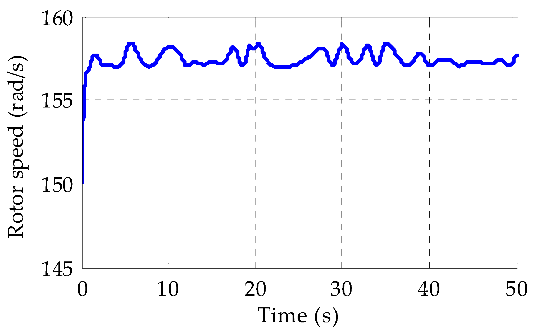
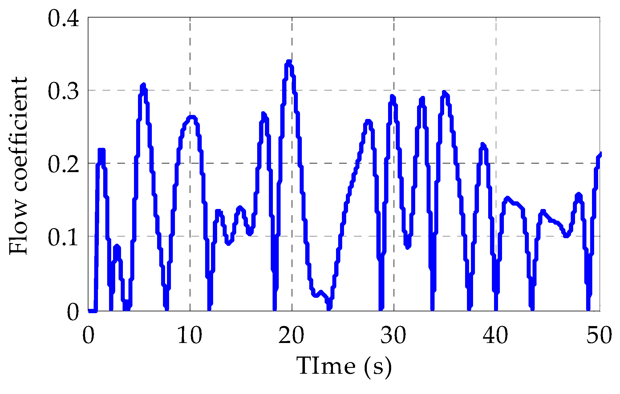
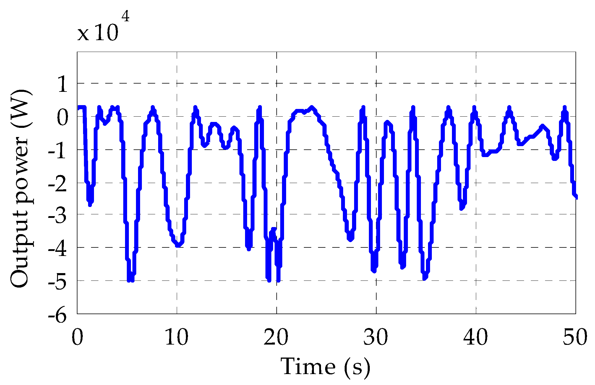
5.1. Performance of the Uncontrolled OWC Plant

In this subsection, the performance of the uncontrolled OWC plant is analyzed in terms of the turbine rotor speed, turbine flow coefficient and electrical output power. As shown in Figure 7, the rotor speed is around 157 rad/s due to the stall of the Wells turbine. It is also evident in the waveform of the flow coefficient in Figure 8 that the flow coefficient crosses the 0.3 threshold value and in those instances turbine stalling occurs. This produces less turbine torque resulting in a reduced output power. The output power at 20 s in Figure 9 suddenly reduces due to the stalling of the turbine and remains below 50 kW. The stalling can be avoided by keeping the flow coefficient below 0.3. For this, the MPPT algorithm and controller is required which is discussed in the next subsections.

5.2. Performance of the PSO-BSC controlled OWC Plant

The PSO [41,42] is a widely used optimization algorithm and used in this study for comparing its performance with the AO algorithm. The PSO technique minimizes the fitness function, $J_{fit}$, and generates the suitable values of BSC unknown parameters, ${\sigma }_1$ and ${\sigma }_2$ with a range of ${\sigma }_1$ and ${\sigma }_2$ as $0<{\sigma }_1, {\sigma }_2<50$. The total number of iterations taken was 50 and other PSO parameters were taken from [43]. The values of the BSC parameters are: ${\sigma }_1=7.6309$ and ${\sigma }_2=6.9962$.

Next, the rotor reference speed (red colored line) as shown in Figure 10 is generated from the MPPT algorithm. The reference rotor speed depends on the air velocity inside the turbine duct. The air velocity is given to the MPPT algorithm which generates the reference rotor speed. The reference rotor speed varies according to changes in the peak air velocity. The actual rotor speed (blue dashed line) as shown in Figure 10a is generated due to the BSC scheme. The actual rotor speed very closely follows the reference speed as shown in Figure 10b. Due to variations in the actual rotor speed according to the reference, the turbine flow coefficient (in Figure 11) is restricted below the 0.3 value and thus, turbine stalling is blocked. Therefore, the output power (in Figure 12) gets maximized and reaches a peak value of 72 kW. It was limited to 50 kW in an uncontrolled OWC plant.

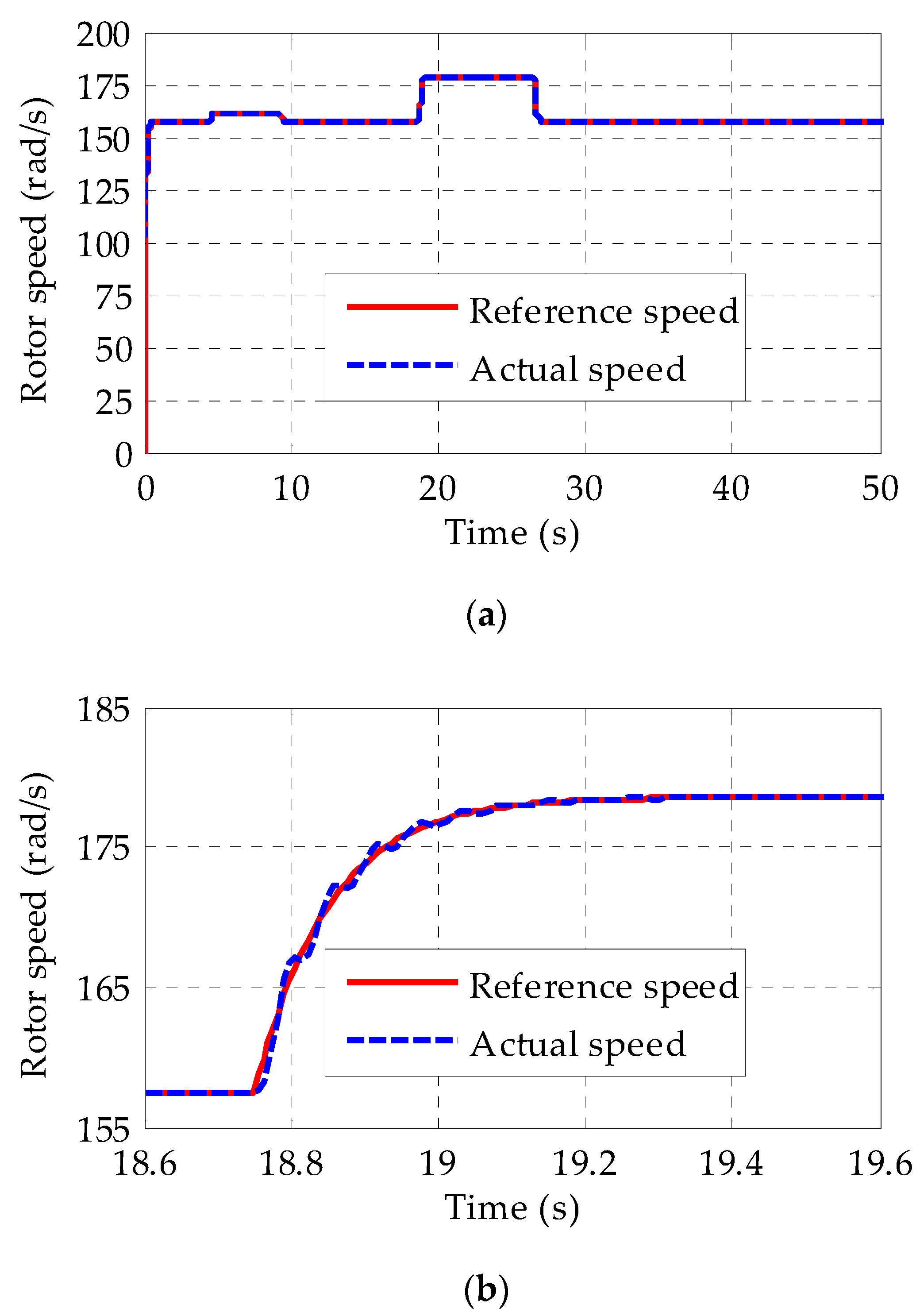
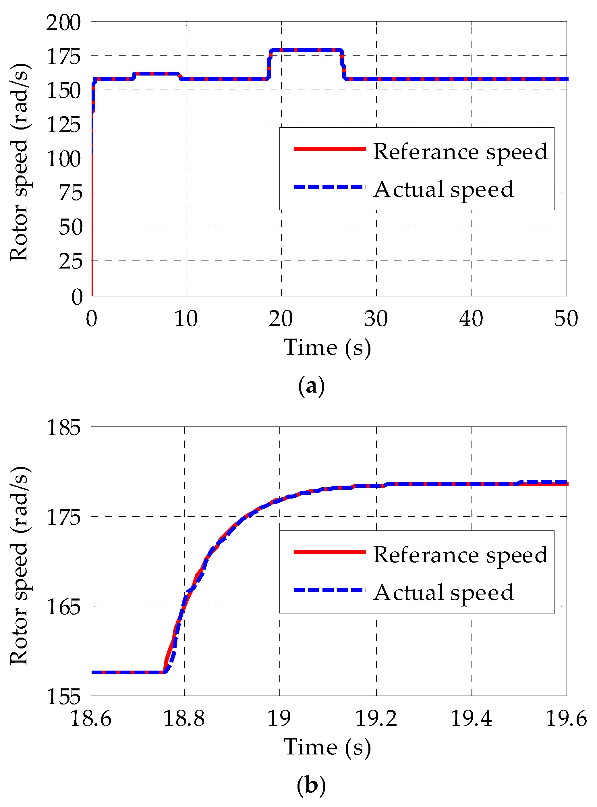
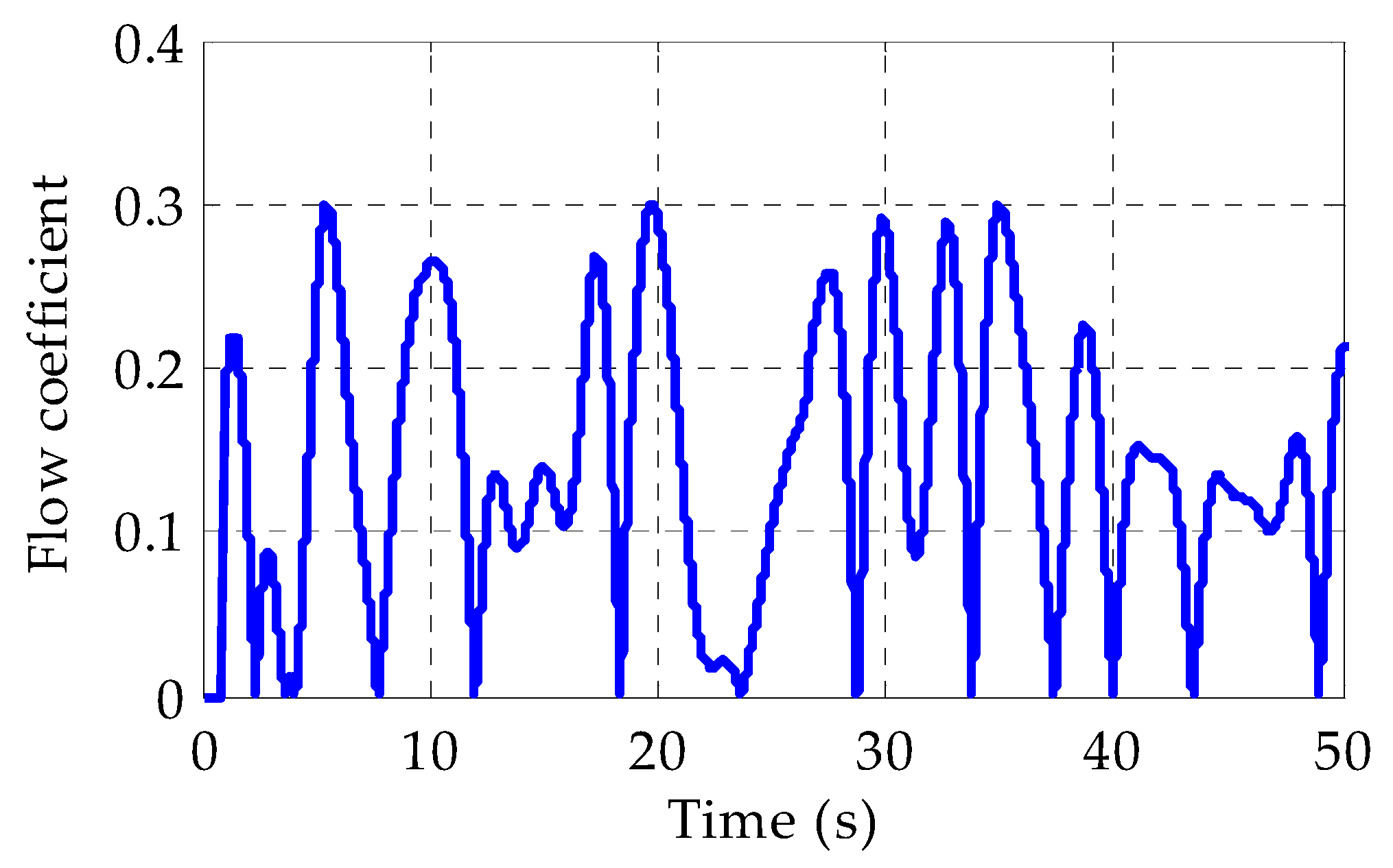
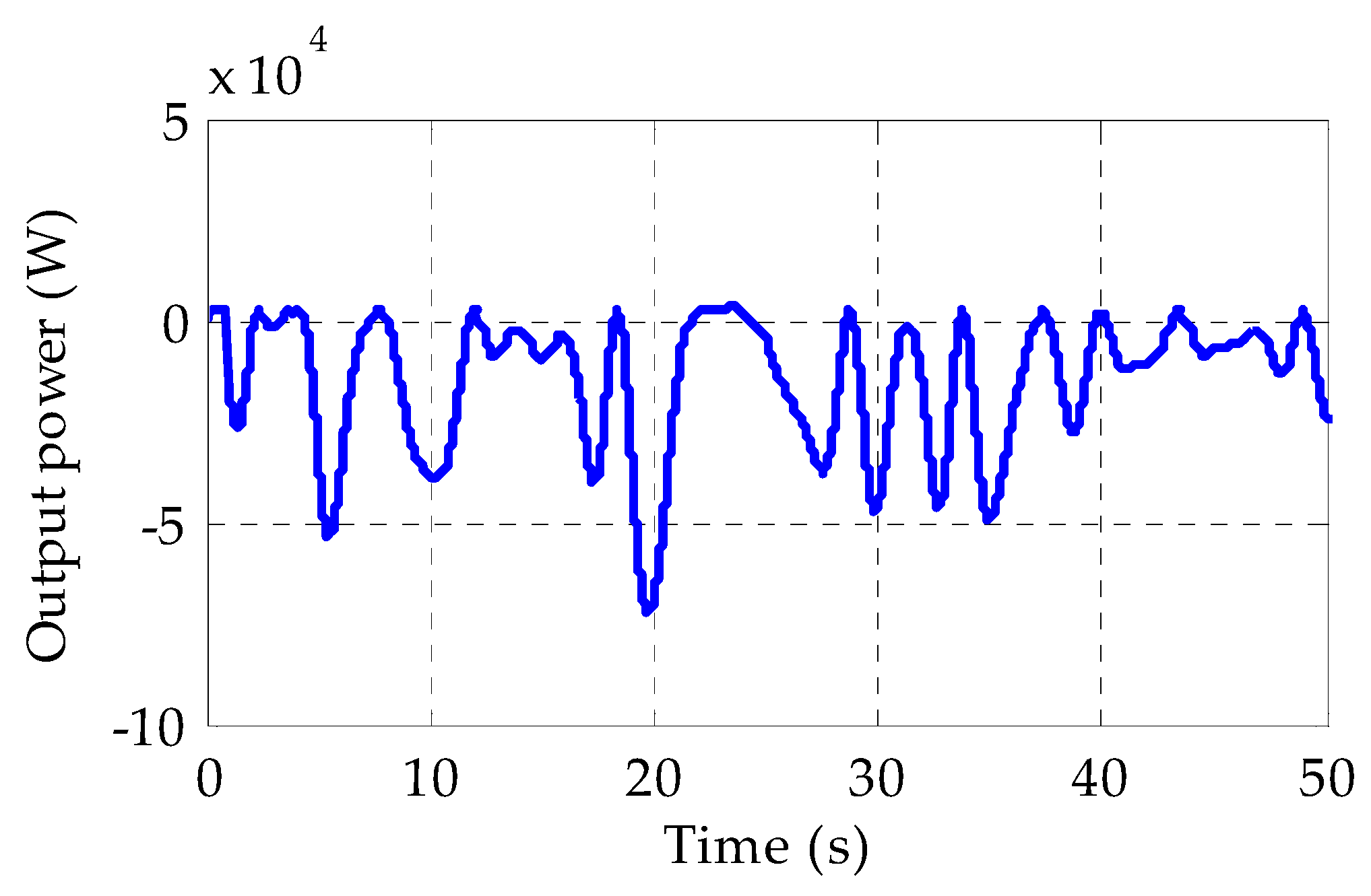
5.3. Performance of the AO-BSC Controlled OWC Plant

The AO technique is a population-based optimization approach inspired by the Aquila’s behaviors in nature during the process of catching prey. The AO technique again minimizes the fitness function, $J_{fit}$, and generates the suitable values of the BSC unknown parameters, ${\sigma }_1$ and ${\sigma }_2$. The AO technique also uses 50 iterations with a range of ${\sigma }_1$ and ${\sigma }_2$ as $0<{\sigma }_1, {\sigma }_2<50$. The values of the optimization parameters of AO technique were taken from [40]. After optimization with AO, the ${\sigma }_1$ and ${\sigma }_2$ are obtained as ${\sigma }_1=5.4581$ and ${\sigma }_2=45.8453$.

The performance of the OWC plant with AO-BSC is shown in Figure 13, Figure 14 and Figure 15. Figure 13a presents the rotor speed performance wherein the actual rotor very closely follows the reference rotor speed. The zoomed version of Figure 13a, as shown in Figure 13b, also shows very close tracking of the reference by actual rotor speed. The turbine stall problem is avoided as the flow coefficient is below the threshold value as shown in Figure 14. Because of this, the output power (in Figure 15) peaks at 72 kW as compared to 50 kW in the uncontrolled case.

5.4. Performance of the GA-BSC Controlled OWC Plant

The GA, which depends on the process of natural selection, the mechanism that propels biological evolution, is a technique for resolving both constrained as well as unconstrained optimization issues. A population of unique solutions is repeatedly modified by the GA [44]. The GA minimizes the fitness function, $J_{fit}$, and generates the optimized values of BSC parameters, ${\sigma }_1$ and ${\sigma }_2$. The GA technique uses 50 iterations with a range of ${\sigma }_1$ and ${\sigma }_2$ as $0<{\sigma }_1, {\sigma }_2<50$. After optimization with the GA, the ${\sigma }_1$ and ${\sigma }_2$ are obtained as ${\sigma }_1=8.377$ and ${\sigma }_2=27.04$.

Figure 16a represents the performance rotor speed for a GA-BSC controlled OWC plant. Very satisfactory tracking can be observed in Figure 16a which is a zoomed version of Figure 16a. The flow coefficient also remains below the permissible limit (Figure 17) which prevents turbine stalling and in turn, the maximum power is extracted from sea waves (Figure 18).

5.5. Performance Comparison of the AO, PSO and GA OWC Plant

For the uncontrolled OWC plant, the peak electrical power generated is below 50 kW whereas for the AO-BSC, PSO-BSC or GA-BSC controlled OWC plant, the peak electrical power generation reaches up to 72 kW as shown in Figure 12, Figure 15 and Figure 18, respectively. It shows an increase of 44% as compared to the uncontrolled OWC plant. Although the performance of all techniques is appropriate for choosing the BSC parameters, the AO technique has the advantage as compared to PSO and GA. The rotor speed error (${\tilde{\alpha }}_1$ in Equation (22)) performance is shown in Figure 19. It is observed that the error waveform for AO-BSC has the least maximum peak overshoot as compared to PSO-BSC and GA-BSC. As shown in Figure 20, the values of $J_{fit}$ are 55.8455, 56.4184 and 58.2377 for AO, PSO and GA, respectively, after completion of the 50 iterations. The AO technique has a lower fitness value as compared to the PSO and GA techniques. Therefore, it can be concluded that the AO technique seems more suitable as compared to the PSO and GA techniques.

6. Conclusions and Future Scope

This paper proposed ocean wave energy control using the AO technique. An OWC with a Wells turbine and DFIG was chosen for the ocean wave energy conversion. For achieving the maximum power, an MPPT algorithm was designed which provided a suitable rotor speed reference to the controller. Then, a nonlinear controller called BSC was designed using the Lyapunov stability theory which helped the actual rotor speed to track the reference speed generated by the MPPT algorithm. The main problem of this study was to choose BSC unknown parameters using optimization methods. For this, an ISE-type fitness function was defined which indirectly depended on BSC parameters. As an objective to minimize the fitness function, the AO technique was employed which resulted in suitable BSC parameters with minimized ISE. The AO result was also compared with the PSO and GA results, where AO outperformed PSO and GA in terms of fitness function value and rotor speed error performance for 50 iterations. The value of the fitness function is 55.8455, 56.4184 and 58.2377 for AO, PSO and GA, respectively, after completion of the 50 iterations. The AO has a minimum fitness function value. Some important OWC plant parameters such as rotor speed, flow coefficient and output power have also been analyzed for an uncontrolled OWC, PSO-BSC, GA-BSC and AO-BSC controlled OWC plant. All optimization techniques perform well in rotor speed tracking, maintaining a flow coefficient below the threshold level, and maximizing output power.

This study employed the AO technique and its comparison with the PSO and GA technique, but many optimization techniques have been developed recently which might be the subject of future research. The parameters of control techniques other than BSC can be optimized using AO and many other optimization methods in future works. The seasonal variations in sea waves could be considered for location specific future studies.

References

1. Kabir, E.; Kumar, P.; Kumar, S.; Adelodun, A.A.; Kim, K.H. Solar energy: Potential and future prospects. Renew. Sustain. Energy Rev. 2018, 82, 894–900. [Google Scholar] [CrossRef]
2. Ferrero Bermejo, J.; Gómez Fernández, J.F.; Olivencia Polo, F.; Crespo Márquez, A. A review of the use of artificial neural network models for energy and reliability prediction. A study of the solar PV 2019, hydraulic and wind energy sources. Appl. Sci. 2019, 9, 1844. [Google Scholar] [CrossRef] [Green Version]
3. Novo, P.G.; Kyozuka, Y. Tidal stream energy as a potential continuous power producer: A case study for West Japan. Energy Convers. Manag. 2021, 245, 114533. [Google Scholar] [CrossRef]
4. Thaeer Hammid, A.; Awad, O.I.; Sulaiman, M.H.; Gunasekaran, S.S.; Mostafa, S.A.; Manoj Kumar, N.; Khalaf, B.A.; Al-Jawhar, Y.A.; Abdulhasan, R.A. A review of optimization algorithms in solving hydro generation scheduling problems. Energies 2020, 13, 2787. [Google Scholar] [CrossRef]
5. Guo, B.; Ahmadian, R.; Falconer, R.A. Refined hydro-environmental modelling for tidal energy generation: West Somerset Lagoon case study. Renew. Energy 2021, 179, 2104–2123. [Google Scholar] [CrossRef]
6. Damacharla, P.; Fard, A.J. A Rolling Electrical Generator Design and Model for Ocean Wave Energy Conversion. Inventions 2020, 5, 3. [Google Scholar] [CrossRef] [Green Version]
7. Portillo Juan, N.; Negro Valdecantos, V.; Esteban, M.D.; López Gutiérrez, J.S. Review of the Influence of Oceanographic and Geometric Parameters on Oscillating Water Columns. J. Mar. Sci. Eng. 2022, 10, 226. [Google Scholar] [CrossRef]
8. Crooks, J.M.; Hewlin Jr, R.L.; Williams, W.B. Computational Design Analysis of a Hydrokinetic Horizontal Parallel Stream Direct Drive Counter-Rotating Darrieus Turbine System: A Phase One Design Analysis Study. Energies 2022, 15, 8942. [Google Scholar] [CrossRef]
9. Hong, Y.; Waters, R.; Boström, C.; Eriksson, M.; Engström, J.; Leijon, M. Review on electrical control strategies for wave energy converting systems. Renew. Sustain. Energy Rev. 2014, 31, 329–342. [Google Scholar] [CrossRef]
10. Ceballos, S.; Rea, J.; Robles, E.; Lopez, I.; Pou, J.; O’Sullivan, D. Control strategies for combining local energy storage with wells turbine oscillating water column devices. Renew. Energy 2015, 83, 1097–1109. [Google Scholar] [CrossRef]
11. Lekube, J.; Garrido, A.J.; Garrido, I. Rotational speed optimization in oscillating water column wave power plants based on maximum power point tracking. IEEE Trans. Autom. Sci. Eng. 2016, 14, 681–691. [Google Scholar] [CrossRef]
12. Henriques, J.C.C.; Gato, L.M.C.; Falcao, A.D.O.; Robles, E.; Faÿ, F.X. Latching control of a floating oscillating-water-column wave energy converter. Renew. Energy 2016, 90, 229–241. [Google Scholar] [CrossRef]
13. Henriques, J.C.C.; Gato, L.M.C.; Lemos, J.M.; Gomes, R.P.F.; Falcão, A.F.O. Peak-power control of a grid-integrated oscillating water column wave energy converter. Energy 2016, 109, 378–390. [Google Scholar] [CrossRef] [Green Version]
14. Mishra, S.K.; Purwar, S.; Kishor, N. An optimal and non-linear speed control of oscillating water column wave energy plant with wells turbine and DFIG. Int. J. Renew. Energy Res. 2016, 6, 995–1006. [Google Scholar]
15. Mishra, S.K.; Purwar, S.; Kishor, N. Design of non-linear controller for ocean wave energy plant. Control. Eng. Pract. 2016, 56, 111–122. [Google Scholar] [CrossRef]
16. Lekube, J.; Garrido, A.J.; Garrido, I.; Otaola, E.; Maseda, J. Flow control in wells turbines for harnessing maximum wave power. Sensors 2018, 18, 535. [Google Scholar] [CrossRef] [PubMed] [Green Version]
17. Mishra, S.K.; Purwar, S.; Kishor, N. Event-triggered nonlinear control of OWC ocean wave energy plant. IEEE Trans. Sustain. Energy 2018, 9, 1750–1760. [Google Scholar] [CrossRef]
18. M’zoughi, F.; Bouallegue, S.; Garrido, A.J.; Garrido, I.; Ayadi, M. Fuzzy gain scheduled PI-based airflow control of an oscillating water column in wave power generation plants. IEEE J. Ocean. Eng. 2018, 44, 1058–1076. [Google Scholar] [CrossRef]
19. M’zoughi, F.; Garrido, I.; Garrido, A.J.; De La Sen, M. Self-adaptive global-best harmony search algorithm-based airflow control of a wells-turbine-based oscillating-water column. Appl. Sci. 2020, 10, 4628. [Google Scholar] [CrossRef]
20. M’zoughi, F.; Garrido, I.; Garrido, A.J. Symmetry-breaking for airflow control optimization of an oscillating-water-column system. Symmetry 2020, 12, 895. [Google Scholar] [CrossRef]
21. M’zoughi, F.; Garrido, I.; Garrido, A.J.; De La Sen, M. ANN-based airflow control for an oscillating water column using surface elevation measurements. Sensors 2020, 20, 1352. [Google Scholar] [CrossRef] [PubMed] [Green Version]
22. Maria-Arenas, A.; Garrido, A.J.; Rusu, E.; Garrido, I. Control strategies applied to wave energy converters: State of the art. Energies 2019, 12, 3115. [Google Scholar] [CrossRef] [Green Version]
23. Henriques, J.C.C.; Portillo, J.C.C.; Sheng, W.; Gato, L.M.C.; Falcão, A.D.O. Dynamics and control of air turbines in oscillating-water-column wave energy converters: Analyses and case study. Renew. Sustain. Energy Rev. 2019, 112, 571–589. [Google Scholar] [CrossRef]
24. Mishra, S.K.; Appasani, B.; Jha, A.V.; Garrido, I.; Garrido, A.J. Centralized Airflow Control to Reduce Output Power Variation in a Complex OWC Ocean Energy Network. Complexity 2020, 2020, 2625301. [Google Scholar] [CrossRef]
25. Mishra, S.K.; Appasani, B.; Verma, V.K.; Jha, A.V.; Kumar, M.R.; Pati, A. PID Control of the OWC Plant to Improve Ocean Wave Energy Capture. In Proceedings of the 2020 IEEE 9th Power India International Conference (PIICON), Sonepat, India, 28 February–1 March 2020; IEEE: New York City, NY, USA, 2020; pp. 1–6. [Google Scholar]
26. M’zoughi, F.; Garrido, I.; Garrido, A.J.; De la Sen, M. Fuzzy gain scheduled-sliding mode rotational speed control of an oscillating water column. IEEE Access 2020, 8, 45853–45873. [Google Scholar] [CrossRef]
27. Napole, C.; Barambones, O.; Derbeli, M.; Cortajarena, J.A.; Calvo, I.; Alkorta, P.; Bustamante, P.F. Double fed induction generator control design based on a fuzzy logic controller for an oscillating water column system. Energies 2021, 14, 3499. [Google Scholar] [CrossRef]
28. Magaña, M.E.; Parlapanis, C.; Gaebele, D.T.; Sawodny, O. Maximization of Wave Energy Conversion into Electricity Using Oscillating Water Columns and Nonlinear Model Predictive Control. IEEE Trans. Sustain. Energy 2021, 13, 1283–1292. [Google Scholar] [CrossRef]
29. Gaebele, D.T.; Magana, M.E.; Brekken, T.K.; Henriques, J.C.; Carrelhas, A.A.; Gato, L.M. Second order sliding mode control of oscillating water column wave energy converters for power improvement. IEEE Trans. Sustain. Energy 2020, 12, 1151–1160. [Google Scholar] [CrossRef]
30. Noman, M.; Li, G.; Wang, K.; Han, B. Electrical control strategy for an ocean energy conversion system. Prot. Control. Mod. Power Syst. 2021, 6, 12. [Google Scholar] [CrossRef]
31. Mishra, S.K.; Mohanta, D.K.; Appasani, B.; Kabalci, E. OWC-Based Ocean Wave Energy Plants; Springer: Singapore, 2021. [Google Scholar]
32. Suchithra, R.; Samad, A. Control of Wave Energy Converters. In Ocean Wave Energy Systems: Hydrodynamics 2021, Power Takeoff and Control Systems; Springer International Publishing: Cham, Switzerland, 2021; pp. 471–486. [Google Scholar]
33. Roh, C.; Kim, K.H. Deep learning prediction for rotational speed of turbine in oscillating water column-type wave energy converter. Energies 2022, 15, 572. [Google Scholar] [CrossRef]
34. Ciappi, L.; Simonetti, I.; Bianchini, A.; Cappietti, L.; Manfrida, G. Application of integrated wave-to-wire modelling for the preliminary design of oscillating water column systems for installations in moderate wave climates. Renew. Energy 2022, 194, 232–248. [Google Scholar] [CrossRef]
35. Ciappi, L.; Stebel, M.; Smolka, J.; Cappietti, L.; Manfrida, G. Analytical and computational fluid dynamics models of wells turbines for oscillating water column systems. J. Energy Resour. Technol. 2022, 144, 050903. [Google Scholar] [CrossRef]
36. Wang, Z.; Wu, S.; Lu, K.H. Improvement of Stability in an Oscillating Water Column Wave Energy Using an Adaptive Intelligent Controller. Energies 2022, 16, 133. [Google Scholar] [CrossRef]
37. Darwish, A.; Aggidis, G.A. A Review on Power Electronic Topologies and Control for Wave Energy Converters. Energies 2022, 15, 9174. [Google Scholar] [CrossRef]
38. Silva, J.M.; Vieira, S.M.; Valério, D.; Henriques, J.C. GA-optimized inverse fuzzy model control of OWC wave power plants. Renew. Energy 2023, 204, 556–568. [Google Scholar] [CrossRef]
39. Carrelhas, A.A.D.; Gato, L.M.C.; Henriques, J.C.C. Peak shaving control in OWC wave energy converters: From concept to implementation in the Mutriku wave power plant. Renew. Sustain. Energy Rev. 2023, 180, 113299. [Google Scholar] [CrossRef]
40. Abualigah, L.; Yousri, D.; Abd Elaziz, M.; Ewees, A.A.; Al-Qaness, M.A.; Gandomi, A.H. Aquila optimizer: A novel meta-heuristic optimization algorithm. Comput. Ind. Eng. 2021, 157, 107250. [Google Scholar] [CrossRef]
41. Poli, R.; Kennedy, J.; Blackwell, T. Particle swarm optimization: An overview. Swarm Intell. 2007, 1, 33–57. [Google Scholar] [CrossRef]
42. Clerc, M. Particle Swarm Optimization; John Wiley & Sons: Hoboken, NJ, USA, 2010; Volume 93. [Google Scholar]
43. Mishra, S.K.; Chandra, D. Stabilization and tracking control of inverted pendulum using fractional order PID controllers. J. Eng. 2014, 2014, 752918. [Google Scholar] [CrossRef] [Green Version]
44. Golberg, D.E. Genetic Algorithms in Search, Optimization, and Machine Learning; Addison Wesley: Boston, MA, USA, 1989; p. 36. [Google Scholar]
Figure 1. Schematic representation of OWC plant.
Energies 16 04495 g001
Figure 2. JONSWAP wave spectrum.
Energies 16 04495 g002
Figure 3. Turbine characteristics.
Energies 16 04495 g003
Figure 4. Block diagram for optimizing BSC parameters based on AO.
Energies 16 04495 g004
Figure 5. JONSWAP irregular wave profile.
Energies 16 04495 g005
Figure 6. Air velocity due to JONSWAP irregular wave profile.
Energies 16 04495 g006
Figure 7. Rotor speed of the uncontrolled OWC plant.
Energies 16 04495 g007
Figure 8. Turbine flow coefficient of uncontrolled OWC plant.
Energies 16 04495 g008
Figure 9. Output power of uncontrolled OWC plant.
Energies 16 04495 g009
Figure 10. Rotor speed of the PSO-BSC controlled OWC plant. (a) Rotor speed versus time. (b) Zoomed version of (a).
Energies 16 04495 g010
Figure 11. Turbine flow coefficient of PSO-BSC controlled OWC plant.
Energies 16 04495 g011
Figure 12. Output power of PSO-BSC controlled OWC plant.
Energies 16 04495 g012
Figure 13. Rotor speed of the AO-BSC controlled OWC plant. (a) Rotor speed versus time. (b) Zoomed version of (a).
Energies 16 04495 g013aEnergies 16 04495 g013b
Figure 14. Turbine flow coefficient of AO-BSC controlled OWC plant.
Energies 16 04495 g014
Figure 15. Output power of AO-BSC controlled OWC plant.
Energies 16 04495 g015
Figure 16. Rotor speed of the GA-BSC controlled OWC plant. (a) Rotor speed versus time. (b) Zoomed version of (a).
Energies 16 04495 g016
Figure 17. Turbine flow coefficient of GA-BSC controlled OWC plant.
Energies 16 04495 g017
Figure 18. Output power of GA-BSC controlled OWC plant.
Energies 16 04495 g018
Figure 19. Rotor speed error performance of AO, PSO and GA.
Energies 16 04495 g019
Figure 20. Iteration wise performance of AO, PSO and GA.
Energies 16 04495 g020