Scientific Approaches to Solving the Problem of Joint Processes of Bubble Boiling of Refrigerant and Its Movement in a Heat Pump Heat Exchanger

Abstract

The joint processes of bubble boiling and refrigerant movement in heat pump tubes are considered. A coil located on the back side of the photovoltaic panel (PVP) is used as an additional heating surface. A mathematical model of the theoretical determination of the temperature on the front surface of the PVP cooled by freon in the coil from the back side has been created. A feature of the numerical simulation of bubble boiling of refrigerant in a coil was the insufficiently detailed study of the process and the lack of references to the results obtained in earlier work. The authors have clarified the boundary conditions and assumptions for numerical simulation of the bubble boiling process of refrigerant R407C. The results were compared with the theoretically found values, and later used in the design of an energy complex consisting of a heat pump and a photovoltaic panel. The mathematical model of theoretical calculation of the PVP temperature and the methodology for constructing a numerical model of bubble boiling of refrigerant as part of the methodology for designing energy technology complexes based on the authors’ plan to present a unified methodology for energy technology complexes for desalination of seawater based on other types of renewable energy sources.

1. Introduction

To date, there are no universal methods for calculating the heat transfer coefficient or a universal description of the thermophysical picture of boiling in a liquid stream. However, many empirical methods have been created for various refrigerants under conditions of low-pressure values (up to 2–4 atm) and mass flow rates, and special formulas for calculating heat transfer to small channels (with a diameter of 1 mm and above) and to strictly specified pressure values have been derived [1,2,3,4,5].

Refrigerant R407C was chosen as the working medium for the study. Its thermodynamic properties are close to the common R22, while it does not contain chlorine, and is non-flammable and non-toxic.

Consider energy complexes that combine heat pumps and the use of solar energy. In the scientific paper [6], the authors developed a system based on solar energy for the production of fresh water and electricity. This system consists of a solar module, a solar-powered Rankine cycle, a heat storage subsystem, and a distillation device. Sea water used for desalination is heated by a saturated steam-water mixture from a steam turbine. Using the outlet liquid as a heat source for the distillation device eliminates the need for an external heat exchanger for condensation. The authors of [6] calculated the energy and exergy efficiency, power and fresh water production capacities for each element of the system. In addition, a parametric study was carried out to take into account environmental conditions.

In research paper [7] the authors analyzed the energy complex for four modules, including a solar heliostat and a receiver, a heat storage device, a Rankine cycle and a desalination system. The steam generator transfers heat to the Rankine cycle. The authors of the study [8] present the balance equations for each element separately and for the entire system as a whole. A mathematical model for the utilization of waste heat from the Rankine cycle has been developed. However, the authors make a number of assumptions: there are no chemical reactions, the potential and kinetic energy practically do not change, the energy costs for the pump are negligible, except for operation in the Rankine cycle, and heat losses occur only through the surface of the reservoir with molten salt and the solar collector.

In [9], the heat loss rate of a solar receiver was calculated. In the research paper [10], after calculating the temperature difference, the authors analyzed the heat losses through the tank with molten salt. The authors of [10] developed a mathematical model of heat accumulation in a tank. This is a rather complicated model, since the volume of the salt melt inside the tank is constantly changing. In [11], a mathematical model of the seawater desalination process was constructed. The study [12] considers the energy and exergy efficiency of the system as a whole. This can be achieved using the main inputs and outputs, while the useful outputs of the system are fresh water and electricity, and the only source of energy is solar energy.

The methodology considered by the authors is a scientific approach to solving the problems of calculating efficiency and optimization in the design of energy technology complexes that combine a heat pump (including a turbo expander for the implementation of the organic Rankine cycle), a photovoltaic panel, a desalination plant, and optionally a solar concentrator and a wind generator. In addition, the scientific approach does not deny the possibility of not only working on the Rankine cycle, since the methodological base does not change. A special feature of the study was the method of heating refrigerant—an additional heater in the form of a coil installed on the back of the photovoltaic panel, Figure 1a,b. Figure 1c also shows the basic scheme of operation of the energy technology complex implemented by the authors. The article considers the first part of the installation—a heat pump.

Let us explain the diagram in Figure 1c. The working substance is refrigerant R407c, which moves along the contour of the system. An evaporator works to convert a gaseous substance into a liquid at low temperature and pressure. The compressor then compresses the liquid refrigerant, increasing the pressure to 19 bar and the temperature to 85 °C. After passing through the compressor, the refrigerant enters the heat exchanger (condenser). Here it gives up its heat to the water, turning it back into a liquid form under pressure. Water enters the system through the filler neck and exits through the drain cock. After the condensed refrigerant passes through the expansion valve, the pressure drops significantly, causing some of the liquid to evaporate. This mixture of liquid and vapor goes to the evaporator. The liquid turns into vapor, evaporating under the action of the heat of the FEP or an additional heater. Due to this, boiling occurs in the evaporator, which consumes heat from the environment.

2. Materials and Methods

2.1. Accepted Assumptions

2.1.1. Vapor-Liquid Mixture

The condensate is throttled before being fed to the evaporator. At the same time, along with a decrease in pressure, the enthalpy constancy (1) can be set with sufficient accuracy.

$$i_1=i_2$$

(1)

The throttling process in the P-i diagram for the selected refrigerant is shown in Figure 2 below in Process 3–4.

Given the necessary pressure drop and knowing the condensation and evaporation temperatures, it is possible to calculate the degree of dryness of steam at point 4, corresponding to the state of refrigerant at the inlet to the evaporator. The degree of dryness under the specified conditions is equal to x = 0.4. Thus, as a mandatory boundary condition, a fraction of 40% of the mass flow rate for steam is set.

2.1.2. Boiling

The calculation takes into account the flow rate in a pipe with a diameter of 5 mm. Developing the previous suggestion, a mix of bubble and foil boiling is assumed. When the liquid boils and evaporates, bubbles form on the walls, which quickly collapse and form a thin film of liquid when there is enough steam in the channel section.

2.1.3. Flow Mode

This flow mode corresponds to the form of a mixture in which steam forms the core of the flow, while the liquid phase flows in the shape of a foil on the surface of the wall. From the first assumption, it can be concluded that the vapor-liquid blend enters the evaporator in the emulsion mode, which is typical for the initial stage of vaporization. Due to the increase in steam consumption (up to a fraction of 0.4, as can be concluded from the diagram in Figure 2) bubbles tend to accumulate and stick together in the flow into larger ones.

It was assumed that the emulsion regime would prevail throughout the site until the formation of steam shells, that is, large steam plugs (Figure 3a). As a result of computer modeling, a similar picture was obtained in the initial formulation of the problem. Figure 3b shows the distribution of the proportion of liquid (red) and steam plugs (gradient to blue) in the tube section. Such a picture was achieved based on the considerations below.

Intensive evaporation of liquid along the boundaries of dry spots (centers of vaporization) is taken as the determining mechanism of bubble boiling. A calculation that takes this factor into account explains the extremely high rate of heat transfer during bubble boiling. When studying a physical model and generalizing experimental data, the analytical Formulas (2) and (3) are adopted for the calculation of heat transfer:

$$q_{boil.}=3.43\cdot {10}^{-4}\frac{{\lambda }^2\Delta T_s^3}{\mathsf{\nu }\sigma T_s}\left[1+\frac{\left(h_g-h_f\right){\left(\Delta T_s\right)}^2}{2R_i{T}_s}\right]\left(1+\sqrt{1+800B}+400B\right)$$

(2)

$$B=\frac{\left(h_g-h_f\right){\left({\mathsf{\rho }}_g\mathsf{\nu }\right)}^{1.5}}{\sigma {\left(\lambda T_s\right)}^{0.5}}$$

(3)

The thermal transfer at boiling in the liquid flow is calculated as a combination of convective heat exchange and heat exchange at boiling with the predominance of the latter (4):

$$q=q_{conv.}+q_{boil.}$$

(4)

The final criterion similarity equation takes the form (5):

$$Nu=\frac{RePr\left(\xi /8\right)}{1+900/Re+12.7{\left(\xi /8\right)}^{0.5}\left(P{r}^{0.67}-1\right)}.$$

(5)

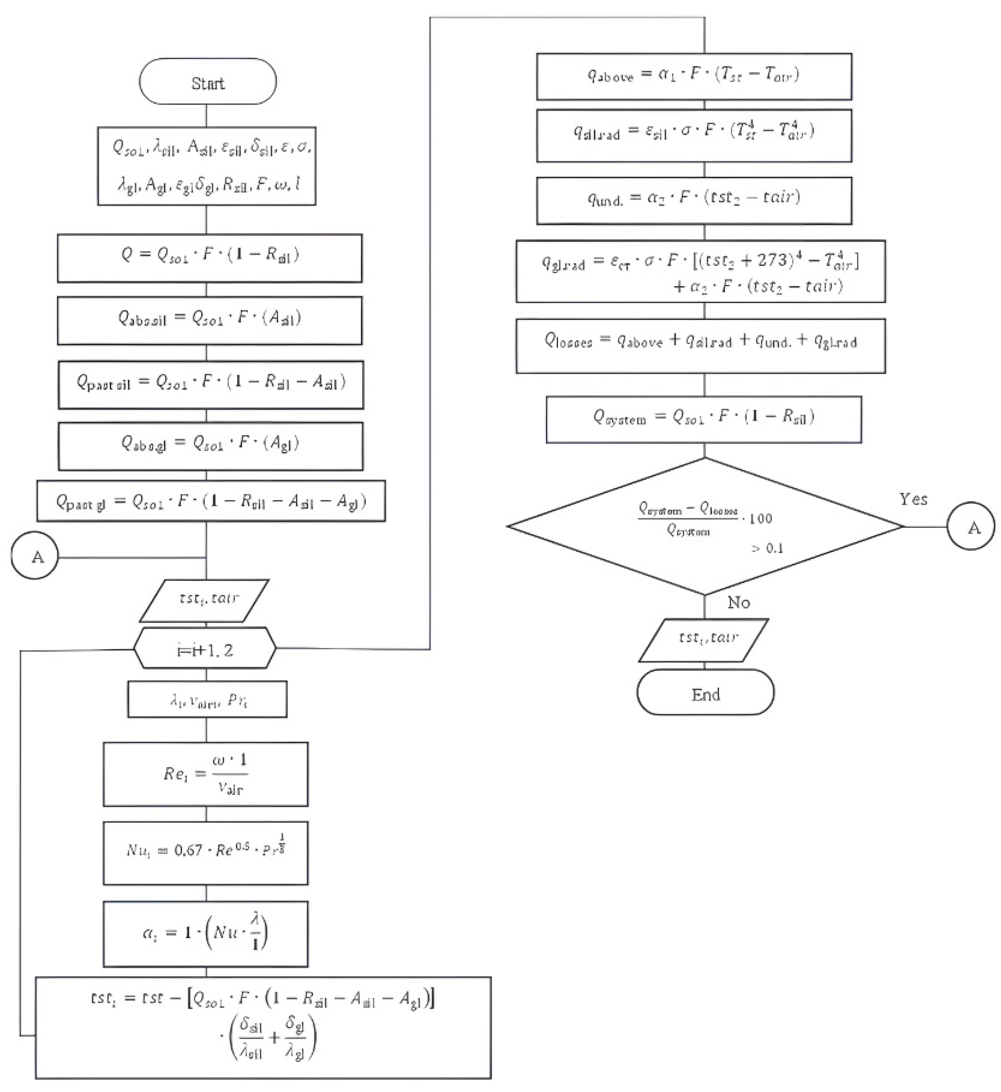
2.2. Theoretical Calculation

2.2.1. The Calculation with Assumptions Is Divided into Two Stages

1. Determining the value of heat entering the system, taking into account losses to the environment;

2. Determination of the refrigerant temperature at the outlet of the evaporator. The first part is presented in the format of a flowchart in Figure 4 according to the Gauss methodology (with input of initial data, forward and reverse, and output of results). As a result, the temperature on the surface of the PVP is calculated with an error of less than 0.1%. The results with an ambient temperature of 20 °C and a wind of 1 m/s are summarized in

Table 1. Calculation data.

Title	Designation	Calculation Formula or Method of Determination	Units of Measurement	Result
Heat flow	Qsol	Given	W/m2	700
Thermal conductivity of silicon	λsil	Given	W/(m2·K)	148
Absorption capacity of silicon	Asil	Given	-	0.2
Degree of silicon blackness	εsil	Given	-	0.71
Silicon thickness	δsil	Given	m	0.001
Stefan-Boltzmann coefficient	σ	Given	W·m−2·K−4	5.67 × 10−8
Thermal conductivity of glass	λgl	Given	W/(m2·K)	0.96
Absorption capacity of glass	Agl	Given	-	0.1
The degree of blackness of the glass	εgl	Given	-	0.93
Glass thickness	δgl	Given	m	0.002
Length and width of the PVP	l	Given	m	0.15675
PVP Square	F	$l^2$	m2	0.025
Reflectivity of silicon	Rsil	Given	-	0.33
Heat absorbed by the PVP	Q	$Q_{sol}\cdot F\left(1-R_{sil}\right)$	W	11.524
Heat absorbed by silicon	Qabs.sil	$Q_{sol}\cdot F\cdot A_{sil}$	W	3.44
Heat passed through silicon	Qpast sil.	$Q_{sol}\cdot F\left(1-R_{sil}-A_{sil}\right)$	W	8.084
Heat absorbed by glass	Qabs.gl.	$Q_{sol}\cdot F\cdot A_{gl}$	W	1.72
Heat passed through the glass	Qpast gl.	$Q_{sol}\cdot F\left(1-R_{sil}-A_{sil}-A_{gl}\right)$	W	6.364
Air velocity	ω	Given	m2/s	1
Thermal conductivity of air	λ	Given	W/(m2·K)	2.4 × 10−2
Air viscosity	νair	Given	m2/s	14.61 × 10−6
Prandtl number for air	Pr	Given	-	0.67
Ambient air temperature	tair	Selected	°C	20
Ambient air temperature	Tair	$t_{air}+273$	K	293
Outside temperature of the PVP	tsur1	Selected	°C	29.12
Outside temperature of the PVP	Tsur1	$t_{\mathrm{sur}1}+273$	K	302.12
Reynolds number	Re1, Re2	$\frac{\omega \cdot 1}{{\mathsf{\nu }}_{air}}$	-	1.073 × 104
Nusselt number	Nu1, Nu2	$0.67R{e}^{0.5}P{r}^{1/3}$	-	60.727
Heat transfer coefficient	α1, α2	$Nu\frac{\lambda }{1}$	W/(m2·K)	9.298
Temperature of the inner surface of the PVP	tsur2	$t_{\mathrm{sur}1}-\left[Q_{sol}\cdot F\left(1-R_{sil}-A_{gl}-A_{gl}\right)\right]$$\times \left(\frac{{\delta }_{sil}}{{\lambda }_{sil}}+\frac{{\delta }_{gl}}{{\lambda }_{gl}}\right)$	°C	29.1
Losses from above	qabove	${\alpha }_1\cdot F\left(T_{\mathrm{sur}1}-T_{air}\right)$	W	2.083
Silicon radiation losses	qsil.rad	${\epsilon }_{sil}\cdot \sigma \cdot F\left(T_{\mathrm{sur}1}^4-T_{air}^4\right)$	W	0.951
Losses from below	qund.	${\alpha }_2\cdot F\left(T_{\mathrm{sur}2}-T_{air}\right)$	W	2.083
Glass radiation losses	qgl.rad	${\epsilon }_{gl}\cdot \sigma \cdot F\left[{\left(T_{\mathrm{sur}2}^{}+273\right)}^4-T_{air}^4\right]$$+Q_{sol}\cdot F\cdot A_{sil}+Q_{coл}\cdot F\cdot A_{gl}$	W	6.399
Heat losses in the system	Qlosses	$q_{above}+q_{sil.rad}+q_{und.}+q_{gl.rad}$	W	11.516
Error rate	ΔQ	$\frac{Q-Q_{losses}}{Q}\cdot 100$	%	0.067

.

A 3D diagram is constructed based on the calculation of the temperature of the PVP wall depending on two input arguments: wind speed and ambient temperature. The result is shown in Figure 5:

The result obtained is used to calculate the temperature on the surface of the evaporator tube (6):

$$t_{\mathrm{ev}.}{}_{\mathrm{wall}}=t_{\mathrm{PEC}\mathrm{wall}}-q\cdot {\displaystyle \sum _{i=1}^n{R}_i}$$

(6)

The temperature on the evaporator wall is a boundary condition for simulating the refrigerant boiling process. For further theoretical calculation, it is a test value when calculating the thermal transmission ratio.

Theoretically, the approximate value of the thermal transmission ratio is calculated according to the Labuntsov formula:

$$\alpha =0.075\left[1+10{\left(\frac{{\mathsf{\rho }}^{″}}{\mathsf{\rho }-{\mathsf{\rho }}^{″}}\right)}^{2/3}\right]{\left(\frac{{\lambda }^2}{\mathsf{\nu }\sigma T_s}\right)}^{1/3}{q}^{2/3}$$

(7)

According to the reference books, the saturation temperature is determined to be T_H under pressure p at point 4 in the diagram according to Figure 2. The physical properties of saturated liquid refrigerant are searched for at the obtained temperature according to reference data [14]. The Reynolds number is calculated at a given flow velocity ω (8):

$$Re=\frac{\omega \cdot d\cdot \mathsf{\rho }}{\mu }$$

(8)

The Nusselt number is calculated according to the Petukhov formula (it implies a developed turbulent regime that will arise due to the presence of turns of the evaporator and high flow velocity of the refrigerant) (9):

$$Nu=0.021R{e}^{0.8}P{r}^{0.43}\epsilon$$

(9)

Next, the convective thermal transmission and boiling heat transfer are compared by comparing the corresponding coefficients. The calculation of the thermal transmission ratio for the forced flow process in the tube is determined as follows (10):

$${\alpha }_{conv.}=\frac{Nu\cdot \lambda }{d}$$

(10)

The thermal transmission ratio for refrigerant boiling is computed according to the equation corresponding to the geometric and thermophysical similarity. Its approximate calculation is performed by Formula (7) under the condition of a boiling pressure above 1 atm.

IF αboil/αconv. > 3, then the thermal transmission ratio during boiling in the pipe is assumed to be equal to αboil, otherwise—αconv.

As a verification condition for the correctness of the selection of the criterion equation, the surface temperature of the evaporator tube is calculated to be higher. The calculation is correct if the temperature value in this part coincides with the previous one (11):

$$t_{ev.}{}_{wall}=\left(T_s-273.15\right)+\frac{q}{{\alpha }_{ev.}}+\frac{q}{2{\lambda }_{wall}}d\cdot \ln \left(\frac{d}{d+2\delta }\right)$$

(11)

To determine the refrigerant temperature at the evaporator outlet, the amount of heat to bring the steam-water mixture to the state of saturated steam is determined, as well as for its overheating (12):

$$Q_{boil.}=\frac{\omega \cdot \mathsf{\rho }\cdot \pi \cdot d^2}{4}r\left(1-x\right)$$

(12)

Evaporation section length (13):

$$l_{ev.}=\frac{Q_{boil.}}{q\cdot \pi \cdot d}$$

(13)

The remaining section is a refrigerant superheater (14):

$$l_{s.h}=l_t-l_{ev.}$$

(14)

The refrigerant outlet temperature is (15):

$$t_{f.out}=\frac{4q\cdot l_{s.h}}{\omega \cdot \mathsf{\rho }\cdot d\cdot c_p^{″}}+T_s-273.15$$

(15)

2.2.2. Comparison of Data from Theoretical Calculation and Analytical Calculation for Temperature

Figure 4 and Formula (15) compared the obtained data. The discrepancy was about 0.1–0.2 °C. Comparison of Data from Theoretical Calculation and Analytical Calculation are presented in

Table 2. Data Comparison.

Wind Speed, m/s	1	5	10
The temperature of the outer wall according to the theoretical calculation, °C	40.74	37.20	34.30
External wall temperature according to analytical calculation, °C	40.57	37.06	34.21

.

2.3. Differential Equations When Solving by Numerical Method

2.3.1. Energy Equations

To apply solutions by the numerical method, the formulas are used:

$$\frac{\partial \left(\mathsf{\rho }{u}_i\right)}{\partial t}+\frac{\partial }{\partial x_j}\left(\mathsf{\rho }{u}_i\mathsf{\rho }{u}_j\right)+\frac{\partial P}{\partial x_i}=\frac{\partial }{\partial x}\left({\mathsf{\tau }}_{ij}+{\mathsf{\tau }}_{ij}^R\right)+S_i$$

(16)

$$\frac{\partial \left(\mathsf{\rho }E\right)}{\partial t}+\nabla \left[V\left(\mathsf{\rho }E+\mathsf{\rho }\right)\right]=\nabla \left[k_{ef}\Delta T-{\displaystyle \sum _j{h}_j{J}_j+{\mathsf{\tau }}_{ef}V}\right]+S_h$$

(17)

2.3.2. The Transfer Equation

Generally used in models with one or two differential equations, the transfer equation can be presented in this form:

$$\mathsf{\rho }\frac{\partial \mathsf{\Phi }}{\partial t}+\mathsf{\rho }\overline{u_j}\frac{\partial \mathsf{\Phi }}{\partial x_j}=P-D+\frac{\partial }{\partial x_j}\left[(\mathsf{\mu }+{\mathsf{\Gamma }}_{\mathsf{\Phi }})\frac{\partial \mathsf{\Phi }}{\partial x_j}\right]+A$$

(18)

The interpretation of the parameters for each type of equations is presented in

Table 3. Explanation of parameters.

	Ф	P	D	Γϕ
Kinetic energy	k	${\mathsf{\tau }}_y\frac{\partial {\overline{u}}_i}{\partial x_j}$	$p\mathsf{\epsilon }$ or ${\mathsf{\beta }}^{\ast }pk\mathsf{\omega }$	$\frac{{\mathsf{\mu }}_t}{{\mathsf{\sigma }}_k}$
Kinetic energy dissipation rate	ε	$c_{\mathsf{\epsilon }1}\frac{\mathsf{\epsilon }}{k}{\mathsf{\tau }}_{ij}\frac{\partial {\overline{u}}_i}{\partial x_j}$	$c_{\mathsf{\epsilon }2}p\frac{{\mathsf{\epsilon }}^2}{k}$	$\frac{u_t}{{\mathsf{\sigma }}_e}$
Specific rate of dissipation	ω	$\mathsf{\alpha }\frac{\mathsf{\omega }}{k}{\mathsf{\tau }}_{ij}\frac{\partial {\overline{u}}_i}{\partial x_j}$	$\mathsf{\beta }p{\mathsf{\omega }}^2$	${\mathsf{\sigma }}_{\mathsf{\omega }}{u}_t$

.

The turbulence model is used in the calculations of transition k-kl-ω.

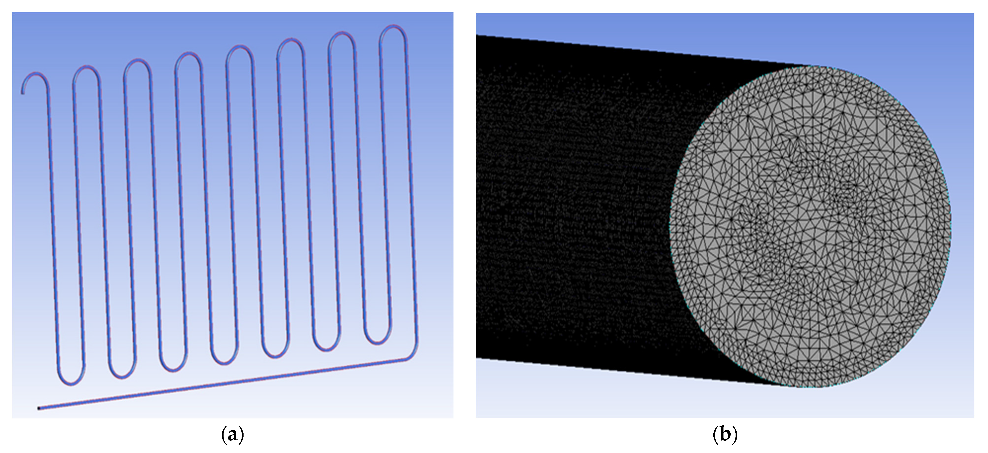
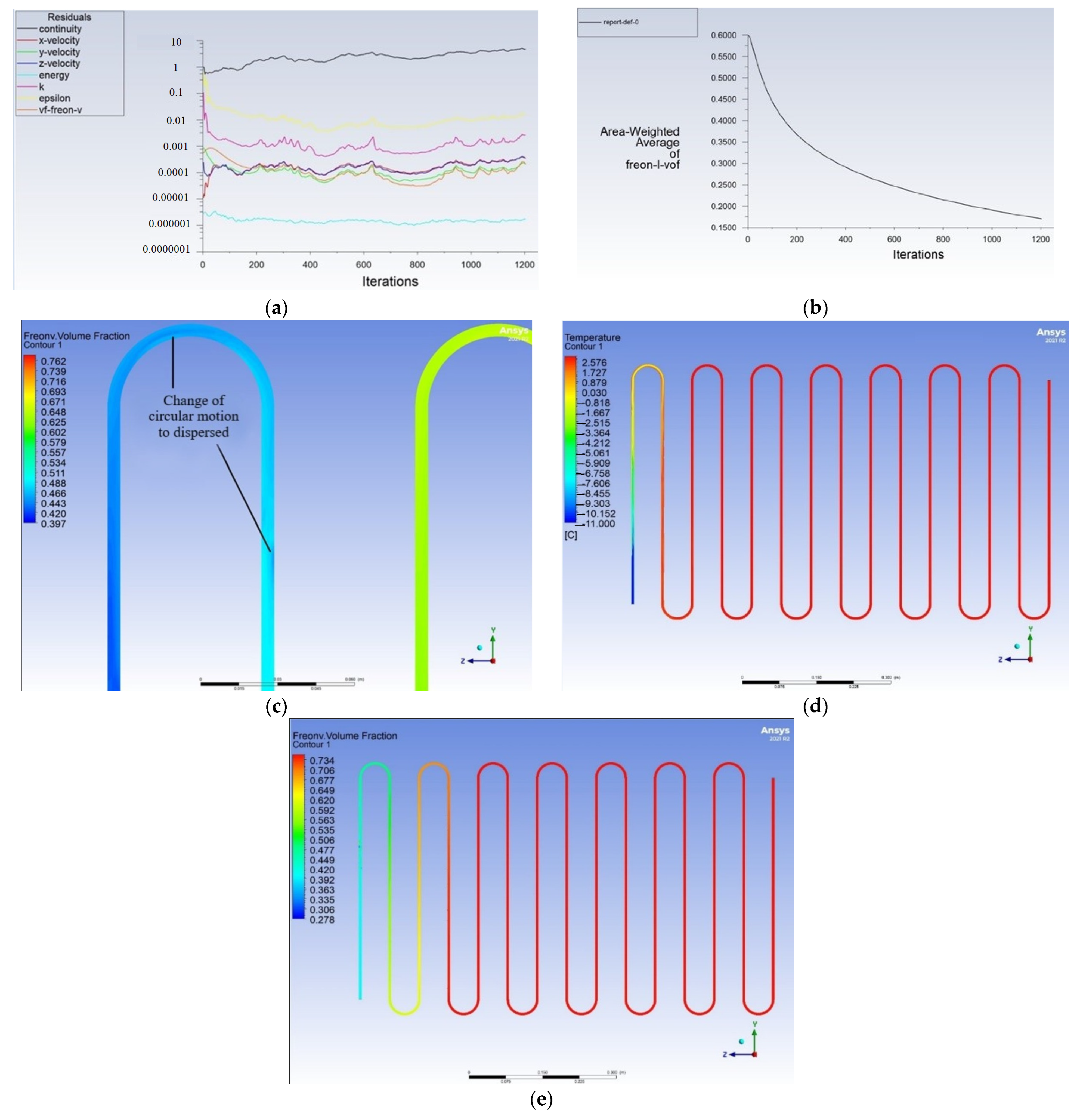
2.4. Modeling in a Software Environment ANSYS Fluent

Standard k-ε (+2E) is a two-parameter RANS model, which is very economical in terms of computational resources and is used for a wide class of flows. Wall functions are used and the model is suitable only for steady turbulent flows. The disadvantage is that in many problems there is a strong eddy diffusion. It should be noted that this model is able to take into account the effect of compressibility and natural convection, which is useful in the calculation of industrial cooling systems. However, this model is not suitable for solving the problem of refrigerant boiling, since it gives a large error and low convergence of results during boiling.

The authors came to the conclusion that transitional flow models should be used (the models only model the transition from laminar to turbulent flow; the wall function is used):

Transition k-kl-ω (+3E)

The k-kl-ω (+3E) transition turbulence model is a widely used turbulence model that combines the k-ε and k-ω models together with the Baldwin–Lomax model. This combination of models provides a reliable method for predicting flow behavior in transients (which is useful in calculating boiling due to its erratic nature and difficult prediction).

The k-kl-ω (+3E) transition model has a number of advantages over other turbulence models. It is able to accurately predict the onset of the transition from laminar to turbulent flow, which is a challenge for many turbulence models.

Transition k-kl-ω (+3E) is a three-parameter model, suitable for solving heat transfer problems in elements that create turbulence (for example, on a turbine blade).

However, the k-kl-ω (+3E) transition model is not without its drawbacks. The model is relatively complex and requires significant computational resources to solve. In addition, it is more prone to numerical instability than other simpler turbulence models, potentially making it difficult to use in some problems. Finally, the model relies on the use of a transition factor to another model, which can lead to inaccuracies and errors if the factor is set incorrectly.

Border conditions

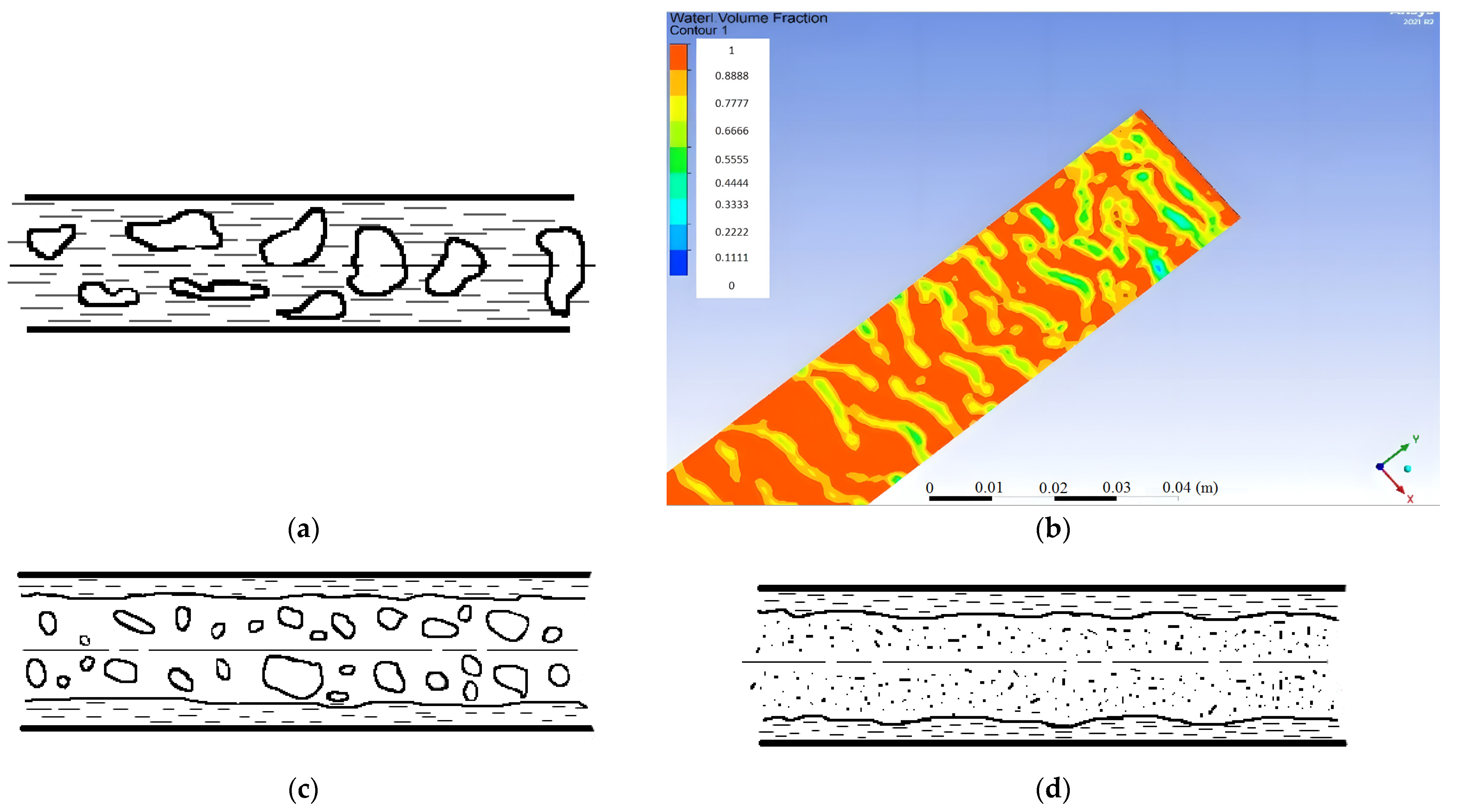
• From the experience of modeling the emulsion flow, the condition of a two-phase flow at the inlet is set (previously, only one liquid phase was set at the inlet, and not a mixture);
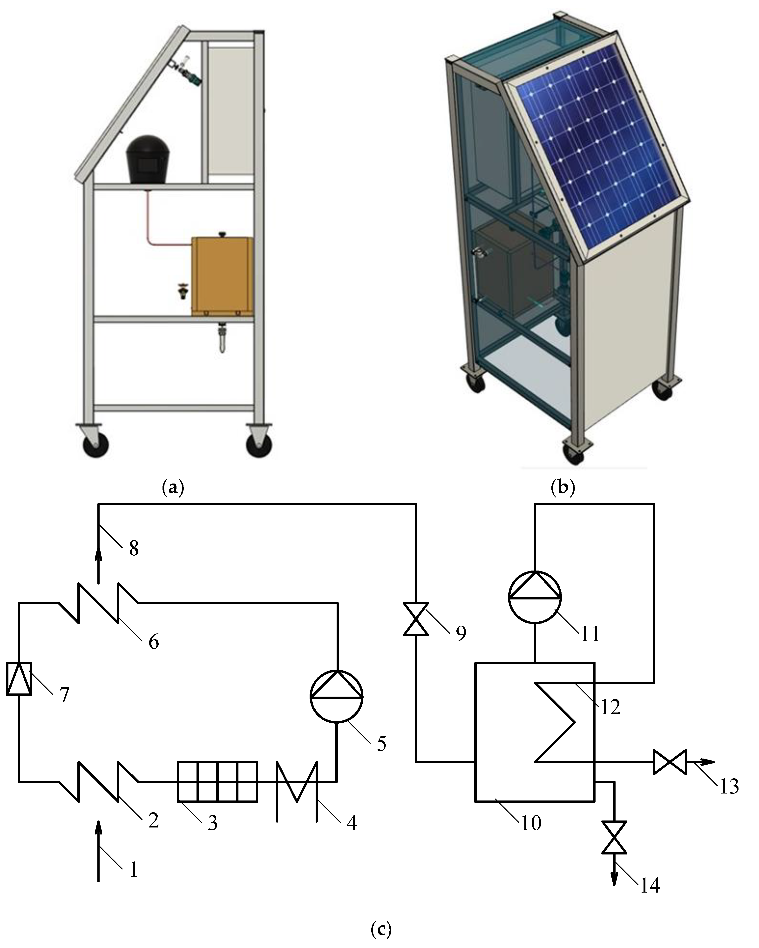
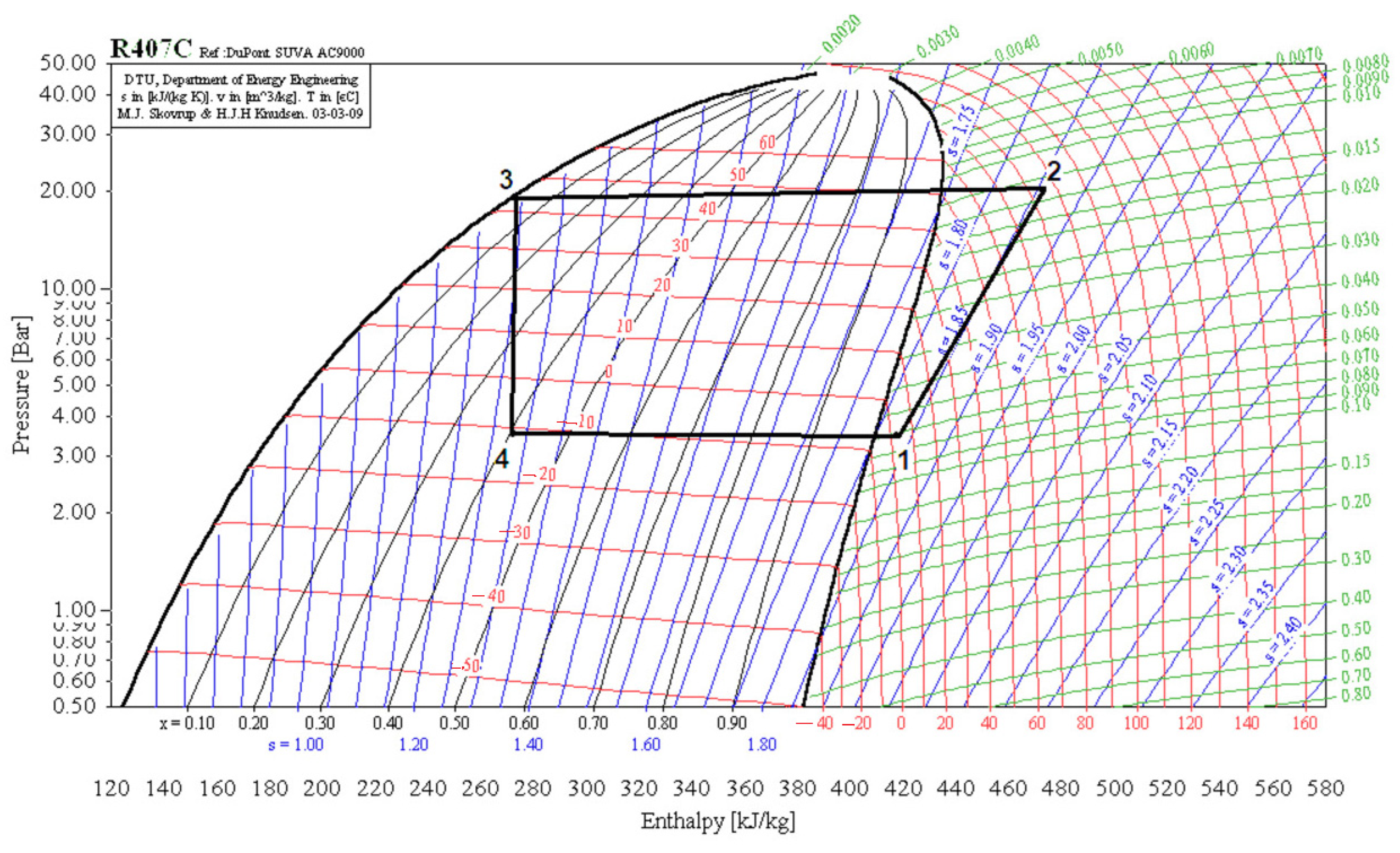
• The extreme pressures in the cycle were determined (3.5 and 19 bar, respectively);
• The saturation temperature is set from the theoretical calculation;
• Based on points 2 and 3, a certain degree of dryness of the vapor-liquid mixture at the inlet to the evaporator is set.

Initial data

−

Element size a: 133.16 × 133.16 × 3 mm, diagonal: 205 mm;

−

Tube inner diameter: 3 mm, tube outer diameter: 5 mm;

−

Temperature on the front surface of the element: 60 °C;

−

Ambient air temperature: 30 °C.

Computer modeling of the flow process of refrigerant R407C in the channel of a brass evaporator with an external diameter of 10 mm and a wall width of 1 mm with a dispersed-ring flow is carried out. Figure 6a shows a geometric model.

The search for unknowns in the equations is carried out using structured and body-adapted prismatic grids (Figure 6b), which allows solving the problem when describing complicated geometry (sweep method for cylindrical bodies; at least 2 million prismatic and tetrahedral elements). A partition in the wall region (a layer of at least three cells) was also performed, which allows using the boundary layer theory for correct calculation of the flow at the walls of the tube, as well as correct calculation of the redistribution of the vapor and liquid phase.

The simulation includes the condition of fluid flow in the gravity field with the formation of vapor bubbles. The group of problems of the effect of the heating wall on the evaporated liquid is solved with satisfactory accuracy by a non-stationary formulation using the Transition k-kl-ω turbulence model. This is a three-parameter model of the RANS group, suitable for a narrow range of tasks, which allows modeling the transformation from laminar to turbulent flow, in which wall functions are used. The main solvable equations embedded in the mathematical model are the energy equation and the turbulence and turbulence-dissipation model equations.

The lifting force (causing the mixing of the flow) occurs due to convection, described by the Boussinesq approximation. This approximation consists in solving the system of Navier–Stokes equations and the energy equation using a special dependence of density on temperature only when calculating the volumetric force.

$$\frac{\partial \tilde{u}}{\partial t}+\left(\tilde{u}\cdot \nabla \right)\tilde{u}=-\frac{1}{{\mathsf{\rho }}_0}\nabla p+\mathsf{\nu }\nabla \tilde{u}-\mathsf{\beta }\mathsf{\theta }\overrightarrow{g}$$

(19)

$$\frac{\partial \mathsf{\theta }}{\partial t}+\tilde{u}\cdot \nabla \mathsf{\theta }=\mathsf{\chi }\Delta \mathsf{\theta }$$

(20)

$$\mathrm{div}\tilde{u}=0$$

(21)

$$\rho (T)={\rho }_0(1-\mathsf{\beta }\mathsf{\theta })$$

(22)

The approximation allows us to take into account the gravity field, that is, the aspiration of steam bubbles in the direction opposite to gravity, respectively, to take into account the orientation of the tube in space.

3. Results

Figure 7 displays the main results of numerical modeling in post-processing. Figure 7a shows that due to the instability of the process, convergence proceeds slowly. However, Figure 7b–d shows the totals for temperatures and fractions of the liquid and vapor phases of refrigerant. The results are indeed close to theoretical and experimental data in accuracy.

It should be noted that there are few research papers devoted to the joint processes of heat transfer, motion and boiling, both in the Russian Federation and in the world today. Basically, scientific laboratories use experimental data obtained earlier on stands and on-site objects. The complexity of research in the field of bubble boiling consists in the transience of processes (high intensity), and a large volume of newly obtained mixtures (for example, the same R407c is a non-azeotropic mixture of three refrigerants). In other words, there are a lot of new artificially produced mixtures, and full-scale work on numerical modeling and verification of at least heat transfer coefficients according to previously obtained formulas and ratios has not been carried out recently. The authors in their works try to partially compensate for the lack of “fresh” data that could be used by both design engineers and research engineers.

Comparison of the Received Data

In the course of the research, the authors were able to compare the temperatures on the back surface of the PVP: obtained experimentally, theoretically, and by numerical modeling. The discrepancy of the data turned out to be acceptable for engineering techniques. The closest results were obtained with theoretical calculation and numerical modeling. The difference was 0.1 °C. At the same time, when compared with experimental data on thermal sensors, the discrepancy is already more significant, approximately 0.3 °C, if we take into account the error of measuring instruments—0.5 °C. However, even with such values of temperature deviations, it is necessary to understand the order of the measured values—from −10 to + 90 °C. That is, with a measurement range of 100 ° C, the error turns out to be insignificant.

Thus, it can be said with confidence that the method of determining the temperature of the PVP and the data introduced into the boundary conditions during numerical modeling open up new opportunities for designers of energy technology complexes based on renewable energy sources, as new scientific approaches to temperature prediction appear, and consequently, more accurate determination of the design features of equipment, in particular, heat exchangers.

Numerical modeling and Formula (15) compared the obtained data. The discrepancy was about 0.1–0.5 °C.

If we compare the results in Table 2 and

Table 4. Data Comparison (compare the results in Table 2 and Table 4).

Wind Speed, m/s	1	5	10
Numerical modeling calculation, °C	40.23	36.94	34.10
External wall temperature according to analytical calculation, °C	40.57	37.06	34.21

, we can conclude that numerical simulation gives results that are closer to the theoretical calculation data, although, for the analytical calculation, the convergence turned out to be quite good.

4. Discussion

4.1. Limitations of the Study

Regarding the limitations of the flow regime under study, it should be noted that after optimizing the mathematical model of heat transfer to the evaporator tube and a number of numerical calculations, it was found that the flow regime in the evaporator is dispersed-annular. Steam in the emulsion mixture is redistributed so that the main phase (liquid with 60% of the flow rate) moves along the pipe surface and in the form of small drops in steam, that is, in an annular mode.

The authors cannot guarantee the applicability of the obtained results for other ratios of the vapor and liquid phases.

4.2. Prospects for the Use of a Heat Pump in an Energy Complex for Seawater Desalination

The goal of creating plants with a thermal process for obtaining fresh water from sea water has led to the development of innovative concepts and design schemes with high efficiency. Particular attention is paid to the issues of optimizing operating modes, replacing expensive structural materials, pipe surfaces with other heater configurations, and reducing scale formation by an increase in the initial temperature of heating demineralized water in order to reduce the consumption of thermal and electrical energy. This goal can be achieved through the utilization of low-grade and waste heat. The cost of water produced in the desalination process is largely determined by the energy source used in the construction of large distillation plants [6,7,8,9,10,11,12].

In the future, the authors will develop a methodology for calculating the exergy fluxes of a desalination plant. An organic Rankine cycle with a turbo expander is used instead of a heat pump for the advanced scheme of the energy complex as a whole, and additional components for the use of renewable energy sources, such as a wind turbine and a solar concentrator, can be implemented. This approach allows for an integrated approach to energy conversion, using multiple sources for maximum efficiency.

First of all, new achievements in the field of low-temperature technology will be considered; for example, the authors of articles [15,16] explore the properties of refrigerant R407c. At the same time, such installations, which are energy technological complexes, must be environmentally friendly. The authors currently have scientific developments in this area. For example, in the article [17], the basics of constructing mathematical models for trigeneration and multigeneration complexes are considered.

5. Conclusions

When optimizing the mathematical model of heat transfer to the evaporator tube and a number of numerical calculations, it was found that the flow regime in the evaporator is dispersed-annular. The steam in the emulsion mixture is redistributed so that the main phase (liquid with a fraction of 60% of the flow rate) moves along the surface of the tube in the form of small droplets in steam—in an annular mode (Figure 2).

As the two-phase flow moves, there is a change to the opposite extreme case, when steam flows along the wall, and the liquid moves in the form of small droplets—in the dispersed mode (Figure 2). The wet steam reaches the saturation state, and then the dry steam overheats (process 4–1 in Figure 1).

It is also revealed that in order to obtain the correct refrigerant heat transfer coefficient for a coil type evaporator, it is necessary to derive a criterion similarity equation based on experimental data.

The results of the calculation of the evaporator with the turbulence model Transition k-kl-ω showed a sufficiently acceptable convergence for engineering computations with the calculation results and empirical data. The discrepancy between the values of the obtained temperatures ranged from 0.1 to 0.5 °C in the measured temperature range 100 °C.

References

1. Romsy, T.; Zacha, P. CFD simulation of upward subcooled boiling flow of freon R12. Acta Polytech. CTU Proc. 2016, 4, 73–79. [Google Scholar] [CrossRef]
2. Milman, O.O.; Ananyev, P.A.; Korlyakova, M.O.; Miloserdov, V.O. Experimental studies of non-stationary thermo-hydraulic processes at freon R113 boiling. J. Phys. Conf. Ser. 2019, 1382, 012114. [Google Scholar] [CrossRef]
3. Kuzmin, A.Y.; Bukin, A.V. Experimental study of heat transfer during boiling on a smooth tube under conditions of free convection of alternative refrigerants R407c and R410a. South Russ. Ecol. Dev. 2010, 5, 121–124. [Google Scholar] [CrossRef]
4. Aleksandrov, A.A.; Orlov, K.A.; Ochkov, V.F. Thermophysical Properties of Working Substances of Heat Power Industry: Internet Reference Book; MPEI Publishing House: Moscow, Russia, 2009. [Google Scholar]
5. Osintsev, K.V.; Alyukov, S.V. Experimental Investigation into the Exergy Loss of a Ground Heat Pump and its Optimization Based on Approximation of Piecewise Linear Functions. J. Eng. Phys. Thermophys. 2022, 95, 9–19. [Google Scholar] [CrossRef]
6. Demir, M.E.; Dincer, I. Development and analysis of a new integrated solar energy system with thermal storage for fresh water and power production. Int. J. Energy Res. 2017, 42, 2864–2874. [Google Scholar] [CrossRef]
7. Demir, M.E.; Dincer, I. Development of an integrated hybrid solar thermal power system with thermoelectric generator for desalination and power production. Desalination 2017, 404, 59–71. [Google Scholar] [CrossRef]
8. Saidur, R.; Elcevvadi, E.; Mekhilef, S.; Safari, A.; Mohammed, H. An overview of different distillation methods for small scale applications. Renew. Sustain. Energy Rev. 2011, 15, 4756–4764. [Google Scholar] [CrossRef]
9. Nafey, A.S.; Mohamad, M.; El-Helaby, S.; Sharaf, M. Theoretical and experimental study of a small unit for solar desalination using flashing process. Energy Convers. Manag. 2007, 48, 528–538. [Google Scholar] [CrossRef]
10. Dincer, I.; Rosen, M.A. Chapter 2—Exergy and Energy Analyses, 2nd, ed.; Dincer, I., Rosen, M.A., Eds.; Elsevier: Amsterdam, The Netherlands, 2013; pp. 21–30. [Google Scholar] [CrossRef]
11. Nasrabadi, A.M.; Korpeh, M. Techno-economic analysis and optimization of a proposed solar-wind-driven multigeneration system; case study of Iran. Int. J. Hydrogen Energy 2023, 48, 13343–13361. [Google Scholar] [CrossRef]
12. Yapicioglu, A.; Dincer, I. A newly developed renewable energy driven multigeneration system with hot silica sand storage for power, hydrogen, freshwater and cooling production. Sustain. Energy Technol. Assess. 2023, 55, 102938. [Google Scholar] [CrossRef]
13. Khrustalev, B.M. Heat and Mass Transfer; BNTU: Minsk, Belarus, 2007; 606p. [Google Scholar]
14. Zalepugin, D.Y.; Tilkunova, N.A.; Chernyshova, I.V.; Vlasov, M.I. Application of Sub- and Supercritical Freons in Xenogenic Bone Matrix Processing. Russ. J. Phys. Chem. B 2017, 11, 1051–1055. [Google Scholar] [CrossRef]
15. Fang, Y.; Wu, M.; Guo, Z.; Ni, H.; Han, X.; Chen, G. Evaluation on Cycle Performance of R161 as a Drop-in Replacement for R407C in Small-Scale Air Conditioning Systems. J. Therm. Sci. 2022, 31, 2068–2076. [Google Scholar] [CrossRef]
16. Deb, S.; Mahesh, K.P.; Das, M.; Das, D.C.; Pal, S.; Das, R.; Das, A.K. Flow boiling heat transfer characteristics over horizontal smooth and microfin tubes: An empirical investigation utilizing R407c. Int. J. Therm. Sci. 2023, 188, 108239. [Google Scholar] [CrossRef]
17. Alabugin, A.; Osintsev, K.; Aliukov, S.; Almetova, Z.; Bolkov, Y. Mathematical Foundations for Modeling a Zero-Carbon Electric Power System in Terms of Sustainability. Mathematics 2023, 11, 2180. [Google Scholar] [CrossRef]
Figure 1. Designed experimental stand: (a) side view (overall dimensions of the stand: height—1706 mm, width—610 mm, depth—642 mm, angle of inclination of the photovoltaic panel—55 degrees, thickness of the photovoltaic panel redesigned for a thickness of 5 mm); (b) isometry; (c) basic diagram of the energy technological complex: Designations are as follows: 1—low-temperature heat source, 2—evaporator, 3—photovoltaic panel, 4—additional (backup) heater, 5—compressor, 6—condenser, 7—expander (capillary tube), 8—heated water, 9—valve, 10—main desalination tank, 11—steam compressor, 12—distillate heat exchanger-condenser, 13—desalinated water outlet, 14—salt water outlet.
Energies 16 04405 g001
Figure 2. Heat pump cycle in the P-i diagram. Symbols and units of measurement: red lines—temperature, °C, blue lines—entropy, kJ/(kg·K), green lines—specific volume, m3/kg, horizontally—enthalpy in kJ/kg, vertically—pressure in bar.
Energies 16 04405 g002
Figure 3. Phase transitions: (a) Emulsion flow mode of the vapor-liquid mixture; (b) Proportion of the liquid phase in the tube cross section, non-dimensional; (c) Ring flow mode (steam inside the liquid); (d) Dispersed flow mode (drops inside the steam). (a,b,d) are borrowed from the literature [13], (c) is the author’s numerical simulation (not described in the literature).
Energies 16 04405 g003
Figure 4. Block diagram of the calculation by the Gauss method. Designations of physical quantities are given in the nomenclature.
Energies 16 04405 g004
Figure 5. Dependence of solar panel wall temperature on ambient temperature and wind speed: the figure was developed by the authors based on the results of theoretical calculation in a specialized dynamic simulation program Math Lab Simulink.
Energies 16 04405 g005
Figure 6. Model building steps: (a) Geometry of the evaporator model; (b) Mesh structure of the evaporator tube.
Energies 16 04405 g006
Figure 7. Post-processing: (a) Fluctuations of the discrepancy calculations of the dispersion-ring mode, non-dimensional; (b) Convergence of the degree of dryness at the evaporator output port, non-dimensional; (c) Mixing of the vapor-liquid mixture (Transition k-kl-ω), non-dimensional; (d) Temperature field (Transition k-kl-ω), °C; (e) Share of vapor in the volume (Transition k-kl-ω), non-dimensional.
Energies 16 04405 g007