
Intensive Data-Driven Model for Real-Time Observability in Low-Voltage Radial DSO Grids
by
 , ,
, ,
Emma M. V. Blomgren
1,* ,
,
Mohsen Banaei
1,
Razgar Ebrahimy
1,
Olof Samuelsson
2,
Francesco D’Ettorre
1 and
Henrik Madsen
1 1
Department of Applied Mathematics and Computer Science, Technical University of Denmark, 2800 Lyngby, Denmark
2
Division of Industrial Electrical Engineering and Automation, Faculty of Engineering, Lund University, SE-22100 Lund, Sweden
*
Author to whom correspondence should be addressed.
Energies 2023, 16(11), 4366; https://doi.org/10.3390/en16114366
Submission received: 23 February 2023
/
Revised: 10 May 2023
/
Accepted: 25 May 2023
/
Published: 27 May 2023
(This article belongs to the Topic Digitalization for Energy Systems)
Abstract
:Increasing levels of distributed generation (DG), as well as changes in electricity consumption behavior, are reshaping power distribution systems. These changes might place particular stress on the secondary low-voltage (LV) distribution systems not originally designed for bi-directional power flows. Voltage violations, reverse power flow, and congestion are the main arising concerns for distribution system operators (DSOs), while observability in these grids is typically nonexistent or very low. The present paper addresses this issue by developing a method for nodal voltage estimation in unbalanced radial LV grids (at 0.4 kV). The workflow of the proposed method combines a data-driven grey-box modeling approach with generalized additive models (GAMs). Furthermore, the proposed method relies on experimental data from a real-world LV grid in Denmark and uses data input from only one measuring device per feeder. Predictions are evaluated by using a test data set of 31 days, which is more than twice the size of the training data set of 13 days. The prediction results show high accuracy at root mean squared errors (RMSEs) of 0.002–0.0004 p.u. The method also requires a short computation time (14 s for the first stage and 2 s for the second stage) that meets requirements for the practical, real-time monitoring of DSO grids.
1. Introduction
As a necessary means towards carbon-neutral energy systems, power systems operation is undergoing a paradigm shift. More devices are becoming electrified, e.g., vehicles and heating devices; the uptake of distributed generation (DG) is increasing; and demand-side flexibility is attracting increasing attention in providing flexibility services for power system operation [1]. These developments are leading to changes in consumption and production patterns, which might stress the low-voltage (LV) distribution power systems that were originally not designed for these conditions. Meanwhile, operational observability in LV grids is generally nonexistent or very low. As a result, to ensure the reliable operation of grids, distribution system operators (DSOs) require techniques to improve grid observability.
Although smart meters are being installed on a large scale in Europe, they offer limited potential for improving the observability of distribution grids. In [2], the authors state that it is not the smart meters that carry the largest cost but rather the required communication infrastructure. Moreover, smart meter communication systems could be subject to cyber-attacks; data are often delayed and not available in near-real time (e.g., residential smart meters that collect data only once a day) and have a slower sampling frequency than phase measurement units (PMUs). Hence, to infer the values of the system’s state variables using a limited number of data, distribution system state estimation (DSSE) is required.
While state estimation is common practice in transmission grids, some factors complicate the application of the same state estimation methods in distribution grids, such as low X/R ratios, unbalanced operation, and fast changes in the configuration of distribution grids [3]. Thus, new methods are proposed in the literature for DSSE that can be categorized from different viewpoints. In general, DSSE problems are voltage-based or branch-current-based. The main focus of this paper is on voltage-based methods. However, several branch-current-based studies can be found in the literature, e.g., [4,5,6].
Among voltage-based DSSE methods, many studies try to apply or modify the weighted least square (WLS) approach as the most commonly used method in transmission system state estimation [7] for DSSE. For instance, Lin et al. [8] proposed a fast decoupled DSSE method taking into account the virtual measurements, i.e., perfect information about the grid, as an equality constraint in the problem formulation. A penalty factor was defined and added to the standard WLS problem that enforces satisfaction of this equality constraint. This method needs no assumptions about voltage magnitudes and phase angles. Chen et al. [9] proposed a methodology for DSSE in cases where only the aggregated data of smart meters are available in order to respect the customers’ privacy. The variance of the smart meters’ measurement errors was used to construct the weight matrix in the WLS optimization problem. A power flow analysis was performed to create time series of active and reactive power data for the study. The problem of DSSE for areas with high numbers of electric vehicles (EVs) was addressed by Nie et al. [10]. To provide more reliable and accurate results, a new quasi-Newton method was used to solve the WLS problem. The effectiveness of the method was evaluated by applying it to the IEEE 14-bus and 30-bus test systems using real travel survey statistics and base load records. Simulation results showed better performance of the proposed method than standard WLS and extended Kalman filter methods, especially when the number of EVs increased. The DSSE solvers of the WLS problems may face the issue of numerical instability and high sensitivity to the choice of initial values. To address this issue, Yao et al. [11] proposed a semi-definitive programming (SDP) approach for the DSSE problem obtained by convex relaxation of the original WLS problem. The method was evaluated by applying it to IEEE 13-bus, 34-bus, and 123-bus test systems. Similarly, Zhu et al. [12] proposed a distributed SDP approach to formulating the DSSE problem, which can be used for areas with several DSOs and minimal data exchange among DSOs due to data confidentiality concerns.
WLS-based approaches are fast and simple, but they could be susceptible to bad data [3]. This has led to the introduction of robust state estimation approaches. Some research papers upgrade the WLS-based approaches to improve the robustness of state estimation. For instance, Wu et al. [13] developed a DSSE method for a grid with limited real-time measurements or with delayed information from smart meters. To provide robust results, a machine learning approach was used to create inputs for the weight matrix of the WLS problem in the state estimator. The test data were generated using power flow analysis at each time interval, and then errors were intentionally added to the system to simulate different measurement errors. Simulation results confirm the robustness of the results against the measurement errors; the type, location, and accuracy of measurements; and the temporary failure of the communication system. Liu et al. [14] proposed a methodology based on the matrix completion approach to perform a robust DSSE. The matrix completion approach uses the known elements in the matrix to estimate the missing elements by solving a rank minimization problem. In the proposed approach, system information is used to form the system state–measurement matrix. The distribution grid model and Ohm’s law are added to the rank minimisation problem as constraints. A decentralized PMU-based robust state estimation method for distribution grids, including a utility grid and several micro-grids, was introduced by Lin et al. [15]. The state estimation problem was formulated as a quadratic optimization problem for the utility grid and micro-grids. Each micro-grid was assumed to be responsible for evaluating its bad data measurements and an iterative algorithm with minimum data exchange between operators was proposed to perform robust DSSE. Fast convergence and scalability are the two main features of this method. Dahale et al. [16] proposed robust formulations for four sparsity-based DSSE approaches (1) 1-D compressive sensing, (2) 2-D compressive sensing, (3) matrix completion, and (4) tensor completion. Simulation results highlight the great performance of compressive-sensing-based approaches compared to tensor completion and matrix completion methods. Furthermore, Raghuvamsi et al. [17] developed a data-driven denoising autoencoder approach for their DSSE model that is robust to false data injection attacks. Their model showed improvements compared to other denoising autoencoder approaches and was able to identify the location of the false data injection and replace the measurements.
Data-driven methods are one of the most recently introduced approaches in DSSE. These methods can be an auxiliary tool in solving the DSSE problem, such as using a neural network (NN) method to generate initial points to solve the main optimization problem [18] or applying machine learning to exploit pseudo-measurements (i.e., artificial measurements, typically acquired from another model or simulated data) [19]. Data-driven approaches could also be used to solve the DSSE problem. NN is one of the most common data-driven approaches for DSSE [20,21,22]. Kim et al. [20] introduced a modified long short-term NN for state estimation in hybrid DC/AC distribution grids. Zamzam et al. [21] proposed a NN method that utilizes the structure of the power grid for DSSE. The proposed architecture reduces the number of coefficients required for mapping from the measurements to the network state, which prevents overfitting and reduces the complexity of the training stage. Among other data-driven approaches, Weng et al. [23] introduced a data-driven DSSE approach that uses the power system patterns and physics to clean data. Supervised learning was used to learn the relationship between the measurement and the system’s state using historical data. Moreover, an approach was suggested to speed up the estimation by 1000 times. To benefit from the advantages of both data-driven and classical methods, Anubi et al. [24] proposed an enhanced resilient DSSE algorithm, which combines a data-driven model with the compressive sensing regression method. Using this algorithm helps the system estimator to recover the true state of the system if faced with false data injection attacks, which mislead regression-based algorithms.
Although the abovementioned studies have covered a wide range of issues and solutions for DSSE, it is worth noting that all these studies are focused on medium-voltage (MV) distribution grids, i.e., voltage levels higher than 0.4 kV. Low-voltage (LV) distribution grids, i.e., 0.4 kV, have characteristics that make them different from MV grids. For instance, LV systems are typically more unbalanced than MV systems. Since customer loads are connected to different phases, uneven load distribution between the phases often arises, marking the need for per-phase voltage estimations. Moreover, MV loads are not as volatile as the aggregate customer loads from the connected LV networks, resulting in lower load variance, supposedly easier to estimate. Additionally, there are DSSE methods for MV distribution grids that rely on more measurements than those that are practically feasible in LV networks. Hence, new methods must be developed for state estimation in LV systems. With this in mind, it is worth mentioning that the authors in [25] developed an NN approach to estimate voltages in a 0.4 kV distribution grid. However, it seems that the method is developed based on confidential customer data, and it could be questioned whether these data inputs should be used for operational purposes. Meanwhile, the reported root mean squared error (RMSE) is 0.59 V and the method requires retraining after 20 days. In [26], the authors derive a method for voltage control in LV grids with high levels of photovoltaic (PV) system uptake, including a remote voltage estimation technique. However, the method relies on the load estimations of customers and the number of customers to produce a generic feeder and is rather designed for voltage control in networks with on-load-tap-changers, limiting the applicability in the context of this study. Mokaribolhassan et al. [27] developed a DSSE method using the augmented complex Kalman filter, also in a power system with PV systems. However, the authors here apply a technique where they separate the PV generation from the customer loads. Testing their model on one month of data for one LV feeder, the authors obtain a mean average error of 0.3% in their simulated studies. Furthermore, in [28], a remote voltage estimation method for radial LV grids is developed, combining a series of power flow calculations and polynomial regression. While the model shows good accuracy, it relies on pseudo-measurements, which can complicate the required retraining of the model; hence, applicable and relevant pseudo-measurements need to be ensured. The model is also tested based on simulated data, and the computation time to fit the model is 0.79 h.
Our comprehensive literature review of DSSE shows that methods for estimating remote voltages in radial LV grids are scarce, as opposed to the many methods found for MV grid DSSE. Furthermore, it would be advantageous in the DSO grid operation to have methods that place an emphasis on providing an estimation of the error components of the model, whereas most methods in the literature focus on mean value prediction. Methods with higher accuracy and a lower computational burden are also crucial for the DSOs to fully realize remote voltage estimation techniques for grid operation. In addition, methods relying on a few measurements that are based on and validated for real-world data are needed. In light of this, the present paper contributes to the field by
- Proposing a data-driven approach for nodal voltage estimation in unbalanced LV grids;
- Combining a grey-box modeling approach to gain explainability and a generalized additive modeling approach to reduce the computational burden significantly, which makes the method practical for online monitoring;
- Deriving the method for a real-world experimental setup and validating the results with high accuracy.
Through the real-world experimental setup, it is ensured that the method is based on input variables that are practical for the DSO to measure because of hardware installations, unlike pseudo-measurements that rely on simulated data. In addition, the experimental setup also includes a new type of electronic measuring device from Linc.world.
The rest of the paper is structured as follows. Section 2 defines the problem. Section 3 provides a generic description of the proposed method. Section 4 describes the experimental setup with electronic measuring devices in a radial LV grid in Denmark. In Section 5, the applied method is presented, including an analysis of the data collected in the experimental setup, a workflow for the model selection process, as well as the applied grey-box and generalized additive modeling approaches. In Section 6, the results from the model selection process are presented and analyzed. The paper is concluded in Section 7 and improvements that could form the basis for future work are also suggested.
2. Problem Definition
During the operation of a radial DSO grid, the end nodes are the most critical regarding voltage stability since the largest voltage drop occurs in this location. Studying different DSO grids, we can see that while there are usually a few end nodes that are equipped with measuring devices, most of the other end nodes are not measured. Estimating the voltage in the end nodes without measurement devices is thus very important.
The model developed in this work is intended to support DSOs in diagnosing the state of the grid during the operation through improved voltage observability. The focus is to develop a method for voltage estimation at the end nodes using the available data from the measuring devices installed in the upper levels and at least one other end node.
The model is further intended to be used in an online monitoring system or integrated into DSOs’ supervisory control and data acquisition (SCADA) systems; thus, priority is given to methods resulting in a low computational burden. We further intend to develop a scalable model for DSO grids, which are generally large grids with many nodes and radial branches, and the goal is to provide reasonable state estimates given input data from a few measurement devices.
3. Workflow of the Proposed Method for Voltage Estimation
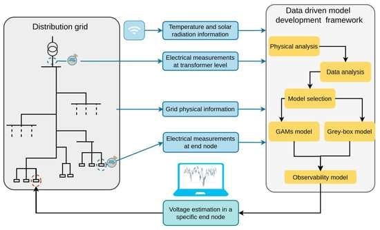
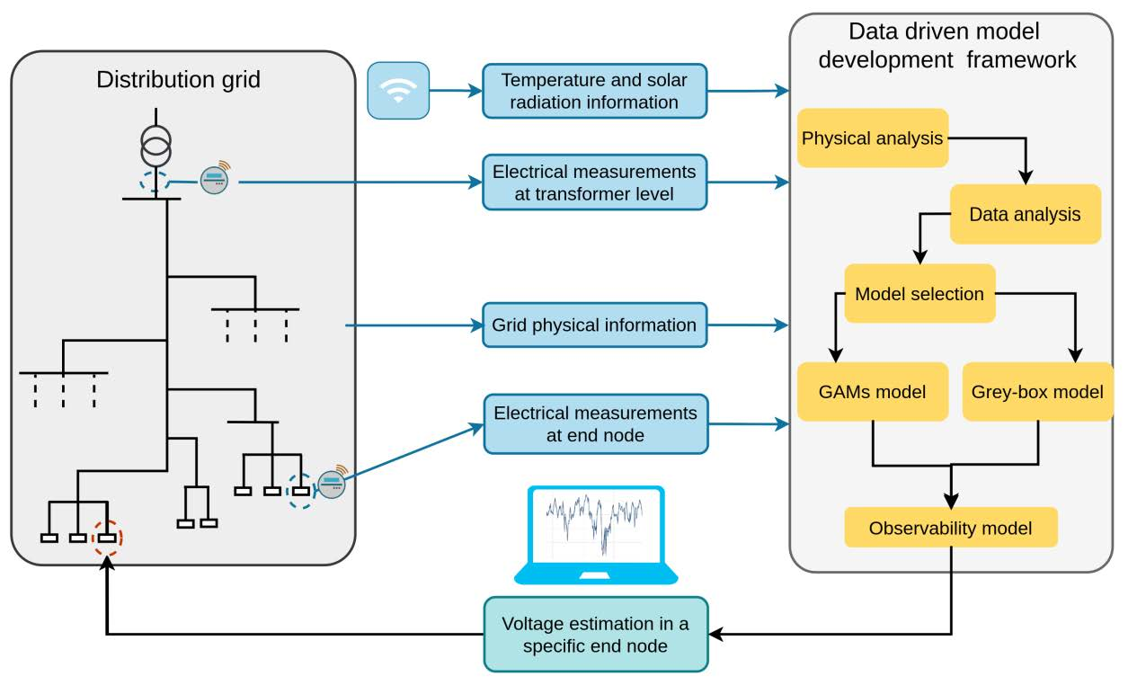
The workflow of the proposed method is illustrated in Figure 1. To build the data-driven model shown in the workflow, in addition to the transformer measurements, we use an end node for which we have data through measurement devices, i.e., an end node with high observability. Then, we adapt the model to estimate voltages at other end nodes without real-time measurements, i.e., the nodes with low observability. The end node was chosen instead of a middle node because it is prioritized in the DSO operation to obtain the end node voltage and the entire voltage drop along one radial feeder with very high certainty through direct measurement, to add robustness to the model setup in case of disturbances.
End node voltage estimation is performed in two steps. First, the proposed workflow is followed to estimate the voltage in a node at the middle of the radial using the data from upper levels and the available data from the end node with high observability. Then, we use the estimated value for the middle node and follow the workflow again to estimate the voltages in other end nodes with low observability.
To perform the voltage estimation, we start with data analysis. In this step, all the data collected from measurement devices, including the available voltage and current measurement data from phases and neutral conductors and weather information, e.g., solar radiation and ambient temperatures, are considered. The information from the data analysis, such as correlation, is then utilized to choose parameters to construct the model.
In the next step, these parameters should be applied to a data-driven approach to perform the voltage estimation. Our investigations indicated that different methods can show different accuracy levels and advantages in voltage estimation at different nodes. Thus, it is suggested to choose two data-driven approaches, (1) a generalized additive model (GAM) and (2) grey-box modeling, for state estimation. For each approach, we apply the data to both approaches, fit the models, evaluate the results, and choose the best model for state estimation.
It is worth mentioning that other time series modeling approaches, such as Autoregressive Moving Average eXogenous (ARMAX) models, could also be alternative modeling techniques. However, GAMs and grey-box models were found to provide satisfactory results for the problem. Therefore, we focus on these approaches in this paper.
Note that the solid arrows in Figure 1 represent the model fitting path of the workflow and might include measurements from more devices for model validation. The idea is that the model fitting could occur when an entire data set is collected by the DSO, e.g., daily. The real-time estimation path of the workflow is represented by the dotted arrows and is based on a few measurement devices and could occur in real time. Thereby, a lower burden on the communication system could be achieved.
Since the proposed method is data-driven and deals directly with data, we cannot present the approach in detail without using real data. Hence, in the next sections, first, the experimental setup is introduced as the case study. Then, the abovementioned approach is applied to this setup step by step to explain how the method should be applied to a real grid. Although there might be differences in applying the method to different grids, such as differences in the parameters with a high correlation or the results of model selection, the main approach will be the same as in Figure 1.
4. Experimental Setup Description
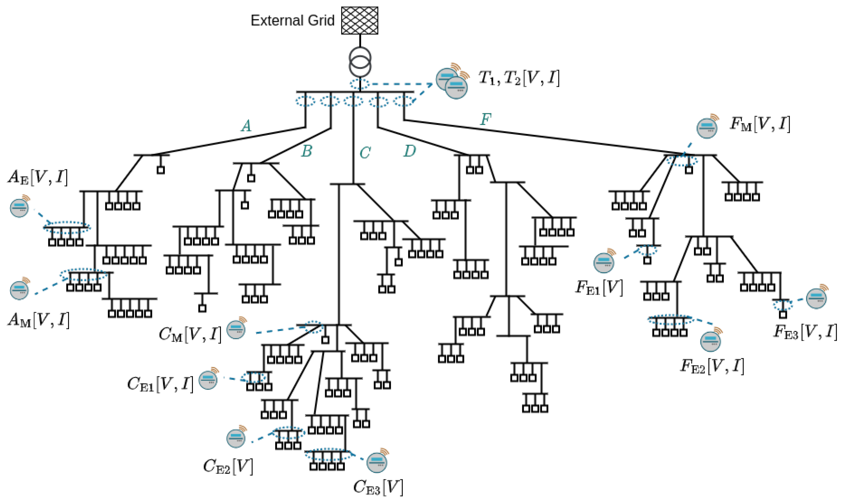
The studied case is a low-voltage (LV) grid at 0.4 kV in Jutland, Denmark, with a 400 VA 10/0.4 kV transformer serving 170 residential customers. In the network, 5–10 customers have electric vehicles (EVs), and 15–20 customers have photovoltaic (PV) systems with rated sizes of 3–6 kW. The households use either district heating or heat pumps for space heating. There are 12 electronic measuring devices installed in the grid, as shown in Figure 2. The electronic measuring devices are placed at the transformer and cable cabinets (cable cabinets are seen as horizontal lines in Figure 2). As seen in the figure, the devices were already installed on three out of the five feeders by the DSO. This research aims to make the best use of these installed measuring devices to perform voltage estimation in end nodes where there is no real-time measuring device installed. It is worth mentioning that the optimal placement of measuring devices in the grid could also be a topic for future studies, but it is beyond the scope of this paper. Due to space limitations in the cable cabinets to install all sensors for the electronic measuring device, some of the devices do not collect current measurements since the DSO prioritizes voltage measurements. Furthermore, the current collecting devices might not measure all in- and outgoing cables from the cable cabinets due to space limitations. Figure 2 indicates which devices collect only voltage measurements and which collect both voltage and current measurements. The devices deliver per-phase data with a one-second resolution. When measuring the current, the devices also measure the active power, power factor, current harmonics, and peak current. The DSO operating the grid has full information on the cable types; thereby, cable impedances and lengths in the grid are known. Active power data from household meters are also available and delivered daily in hourly resolution.
5. Method
The models designed and developed in this research are physics-informed (physics-based) and data-driven. This means that the physics and known theories are used to build the first structure of the model, while the data, together with statistical and analytical tools, guide the process of finding the final model (e.g., a grey-box model). The data reflect the system of interest, including disturbances, which are not always possible to foresee or measure directly. Thus, a probabilistic model that reflects the real-world system, namely the power system in the experimental setup, is achieved. In this section, we first describe the physics of the system utilized to build the end node voltage estimation models, followed by analysis of the data collected in the experimental setup. We then present how generalized additive models (GAMs) and grey-box models are applied in the model selection process.
5.1. Physics of the System—Voltage Drop
Since the model is developed for a radial LV network, the equations that guide the first structure of the model are voltage drop equations. For a meshed network, power flow equations might be more suitable, but due to the low ratio in LV grids, this would directly become a set of non-linear equations.
It should further be noted that the common voltage drop equations are used to calculate line-to-neutral voltage drops [29]. Since the LV grids are unbalanced, the neutral conductor might carry currents; hence, the neutral conductor voltage might not be zero [30,31]. Thus, we will investigate whether a term for the neutral current voltage drop, , should be included in the voltage drop equations such that
where is the sending-end voltage (i.e., the voltage at the node upstream of the network) and is the receiving-end voltage (i.e., the voltage at the node downstream of the network).
Looking at Figure 2, we can see that using the nodes with installed devices as sending-end and receiving-end voltage inputs ( and ) in Equation (1), there will be loads not only at the receiving end but also along the feeder. The effective cable length (or impedance) in the voltage drop equations was discussed in [32], where the authors suggested calculating the load center distance as it varies with the total ampere distribution along the feeder. However, their suggested method becomes impractical for a real-time algorithm as it requires real-time data from all households. Instead, we will fit a parameter in the model, based on available data, that reflects the effective resistance and reactance of the feeder. The resistance also increases with temperature. This might lead to seasonal deviations in the model, which will be investigated as well.
Since distribution networks are quite large and the installation needs to be scalable, another objective of this work is to devise a technique that requires the minimum number of extra measurements from the network. This avoids extra capital investment for the DSOs when rolling out the solution at scale. For example, the distribution network studied in this paper has 22 end nodes. Assuming that the DSO owns 1000 such grids, installing one measurement unit at each end node will result in 22,000 measuring devices, which is an expensive solution. However, if the proposed solution can reduce the number of measurement units to one at each branch, they would only need 5000 units. Turning to classical WLS state estimation is not an option here as it would require more devices to provide enough observability or accurate pseudo-measurements in at least the same time resolution as the model (minimum 10 min). Instead, we use the data at hand to develop a model that estimates the states of concern, i.e., the states at the customer premises.
5.2. Data Analysis
To avoid redundant discussion, the data analysis only presents data for the third phase, L3. The input parameters used in the model selection process are listed in Table 1. The training data set is from 18 April 2022 to 30 April 2022 and the test data set is from 1 May 2022 to 31 May 2022.
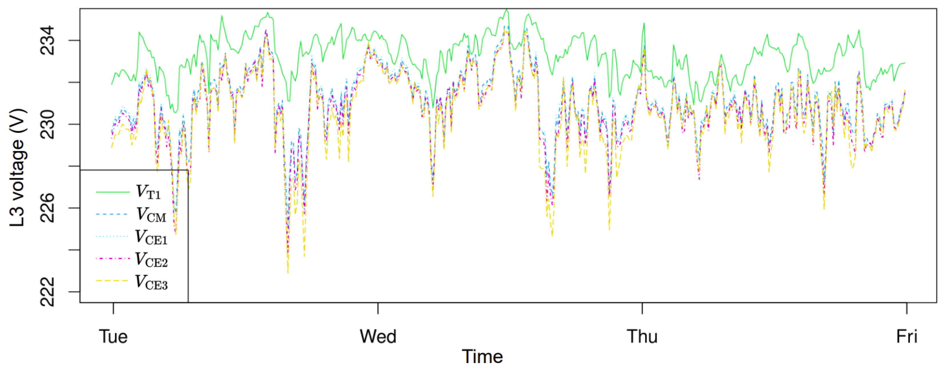
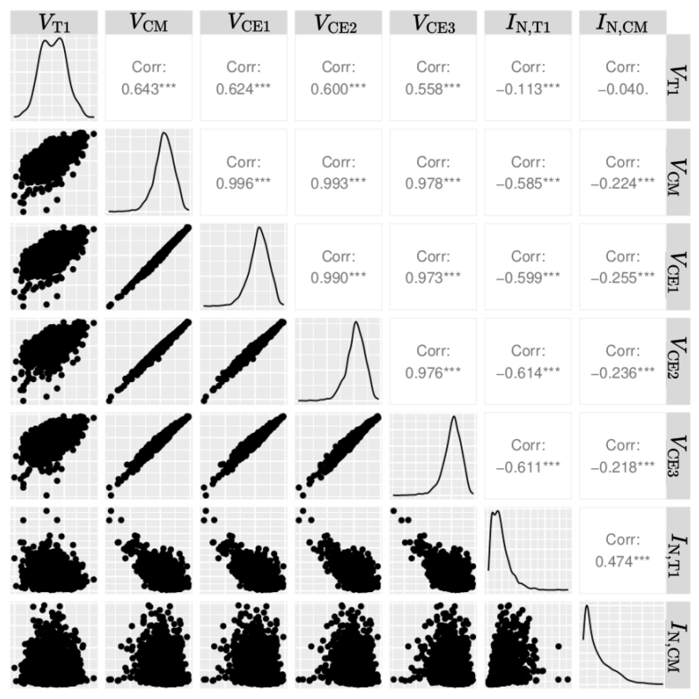
The voltage time series is shown in Figure 3 for feeder C in the grid (see Figure 2). It can be seen that there is a significant voltage drop from the transformer (device ) to the nodes at the edge of the radial (e.g., device ) and that the variations in voltage drop seem quite correlated. In Figure 4, scatter plots and correlations of the same voltage measurements (as in Figure 3) and also the neutral currents along radial C (i.e., ) can be seen. The behavior seen in Figure 3 is further supported by Figure 4, where higher correlations are seen between the node voltages (at , , , and ) than between the nodes and the transformer voltages.
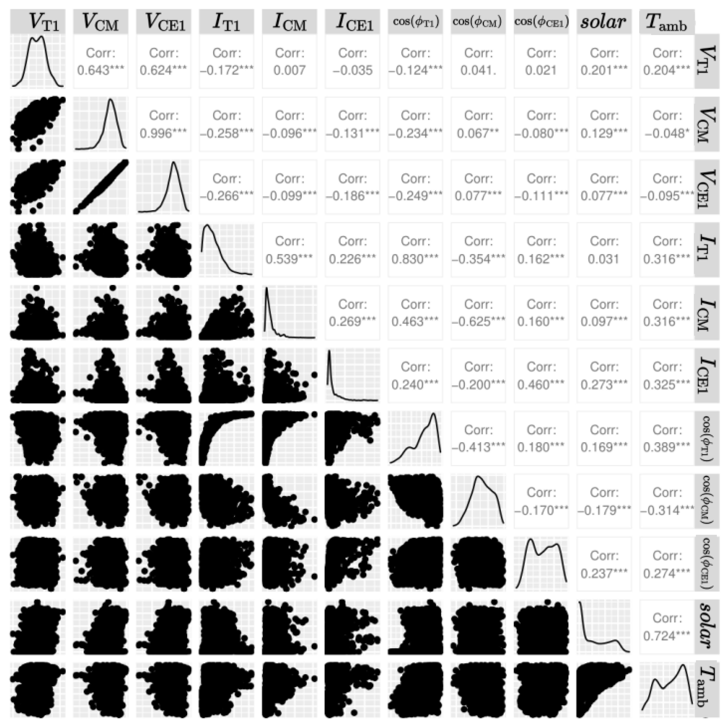
Figure 5 presents scatter plots, data density, and correlations for relevant input parameters. It is noteworthy that although the voltage has a higher correlation with the other edge voltages, the current for has a higher correlation with the edge voltages than the current at . Ambient temperature has a very low correlation and will be excluded as a potential input. Solar radiation, on the other hand, has a higher correlation with the voltages. However, it may not necessarily be an explanatory variable as it probably coincides with a higher load. Therefore, the current should be a better input variable as the voltage drop equation supports it. Nevertheless, this observation will be further investigated in Section 5.4 and Section 5.5. Interestingly, Figure 4 suggests a high correlation between neutral currents and the nodal voltages, which will be further explored in the model selection process.
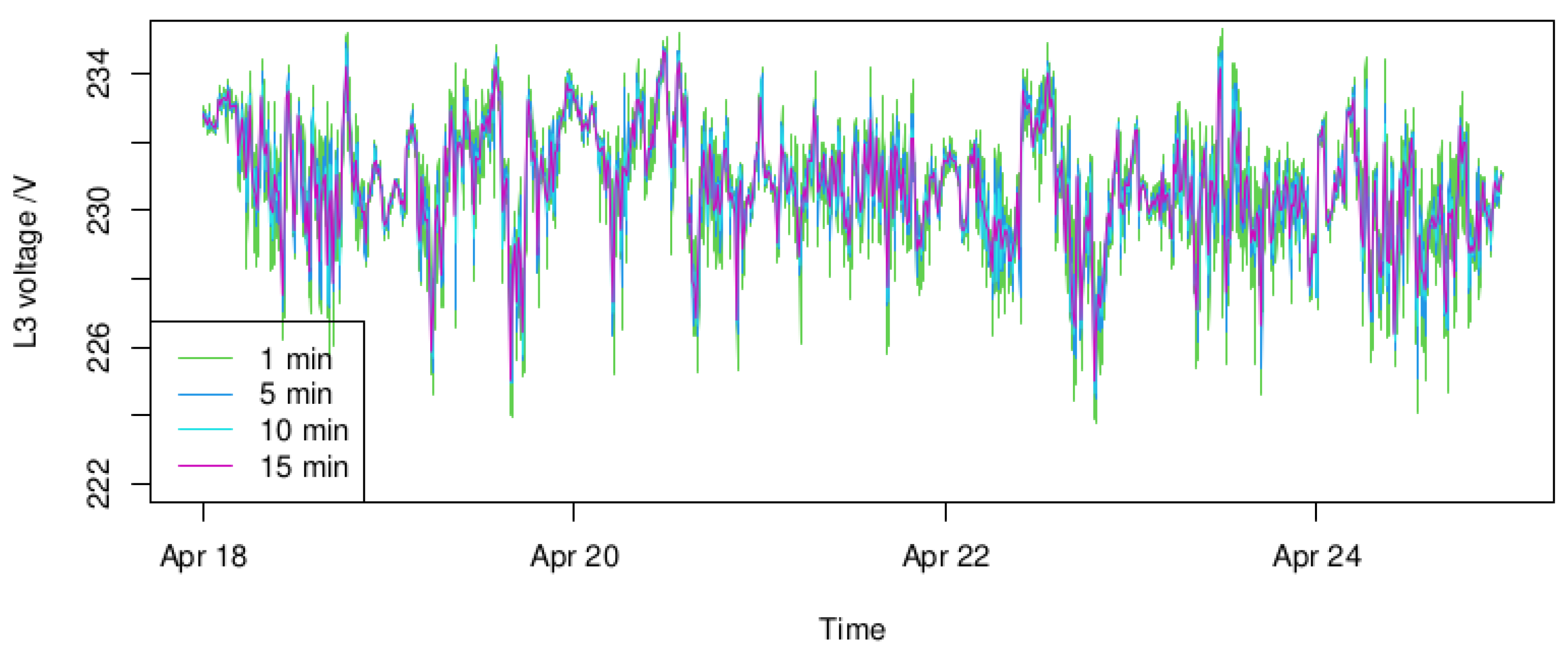
The original data are collected at a 1 second resolution. Therefore, filtering is required to manage the large data set. In Figure 6, filtering to time resolutions of 1, 5, 10, and 15 min can be seen for the third phase voltage. Comparing time resolutions of 1 min to 15 min, it can be seen that the voltage peaks and drops appear smoothed, and the time series is less volatile, which is a natural outcome of low-pass filtering. As persistent voltage peaks and drops are of concern for power system operation to avoid outages, we instead aim to find a suitable model for time resolutions of 5 or 10 min, which should be sufficient for DSO operation while having a manageable data throughput (or computational burden). Voltage data in lower resolutions would be less meaningful for the DSO to detect any voltage stability issues due to the volatile behavior. Higher time resolutions might, on the other hand, result in control strategies that are too volatile and miss the overall voltage behavior over time. However, higher time resolutions could be of interest for other voltage dynamic stability issues, but this is beyond the scope of this paper. Ten-minute filtering is initially chosen to offer the possibility of incorporating environmental data, which have a time resolution of 10 min.
5.3. Model Selection
To build the initial end node voltage estimation model, data collected from feeder C in the grid (see Figure 2) were utilized. As previously stated, one of the objectives of the proposed method was to minimize the number of required measuring devices. However, it was realized early in the model selection process that using only the measurements at the transformer level was insufficient to model the end node voltages. Instead, a workflow using devices at specific locations in the feeder was derived (see Figure 1).
GAM and grey-box modeling approaches were used to build the observability model, which will be discussed in detail in Section 5.4 and Section 5.5. In both approaches, a forward selection process was followed for model evaluation, as described in Section 5.6.
To better understand the workflow, let us consider feeder C in Figure 2 as an example. The goal is to estimate the voltage in one of the end nodes, such as or . To this end, we need one measurement in addition to the measurements in the transformer level. Both and measurements can be used. However, in the case of using , one end node voltage will be known by the DSO with very high accuracy. Furthermore, if the voltage drop along the feeder is known, it will supposedly be easier to derive models for other end nodes in the network. Thus, measurements in transformer and one of the end nodes, e.g., , are used to build the model. Considering the two measurements and node , two voltage drop equations can be expressed as below:
where , , and are the phase-to-ground voltages at devices , , and , respectively. is the voltage drop between devices and , and is the voltage drop between devices and . Both the GAMs and grey-box model structures are derived assuming that is partly described by Equation (2) and partly by Equation (3) such that
where k are measurement instants in time; , a, and b are coefficients to scale the contributions from Equations (2) and (3), respectively; and are independent and identically distributed errors assumed to be Gaussian white noise, . Both modeling approaches start with this formula as an initial model structure.
To estimate the end node voltages at low-observability radial feeders, estimates from a high-observability feeder are then utilized as model inputs.
5.4. GAM Model
GAMs are investigated in this subsection as possible structures to obtain the voltage estimation model. The general expression for GAMs is
where is the expected value of a response variable . represents the parametric part of the model with explanatory variables and parameters , and represents smooth functions of variables [33]. For more details of the GAM models, the reader is referred to [33].
The initially derived GAM model from Equation (4) has the following structure:
where the inputs are described in Table 1 and t is the time variable. and represent smooth functions using B-splines. The parameters were estimated using the gam() and gamm() functions in R package mgcv version 1.8–40 [33,34,35,36,37]. Furthermore, a Gaussian distribution was used.
The initial formula in Equation (6) is derived using only the terms associated with the resistance of the voltage drop equations. Following the data analysis in Section 5.2 and the voltage drop description in Section 5.1, various extensions of the inputs were explored:
- Adding a smooth term relating to the reactive-current term in the voltage drop equation by using the line current and as inputs, where is the power factor measured by device d. This was done to investigate the impact of the reactance in the cable.
- Adding voltage drop terms using and to investigate the impact of the voltage drop in the neutral conductor. It was impossible to use the neutral current data in due to a lack of data availability.
- Adding the temperature as an input by incorporating it into the smooth functions related to cable resistance () to investigate whether the temperature has an impact on the resistance.
- Adding a smooth term for solar radiation to investigate the potential impact of PV panels in the network. Here, a smooth term was used due the complicated functional relationship.
- Adding a seasonal term to investigate whether there is an additional daily or hourly variation not explained by other data. This was done using cubic splines with periodic incremental time step inputs (i.e., a vector …, where m is the period length of a day or hour).
Additionally, variations of the smooth functions were explored.
5.5. Grey-Box Model
Grey-box models were also explored as another modeling approach because they have proven useful when developing data-driven models for physical systems (e.g., in [38,39]). In grey-box models, a known theory of a physical system is used to build the first structure for the model, while statistics and data are used to develop the model further, as well as to estimate the parameters of the model [40]. Thus, it is a mixture of deterministic modeling, relying purely on the known theory, and black-box models, relying purely on statistics and data. Grey-box models, consisting of a set of stochastic differential equations, can be described in a continuous–discrete time state-space representation as follows:
where k are points in time, , of measurements; is the state vector; is the vector of measured outputs; is the vector of input variables; is a vector of unknown parameters; , , and are linear or nonlinear functions; are m-dimensional standard Wiener processes; and are the measurement errors [41]. The Wiener processes are associated with the system error and we assume that they are independent, and the measurement errors are assumed to be Gaussian white noise and uncorrelated to other measurement errors. We further assume that the Wiener processes and the measurement errors are independent.
The initial grey-box model in the model selection process is described as follows:
where k are points in time, , of measurements; a, b, c, and f are parameters to be estimated; and are cable resistances; is the discrete differential of the current at to the previous time step, i.e., (since only discrete measurements are available); consequently, is the discrete differential of the current at () and other inputs are described in Table 1. Note that the time indices in the system equations are omitted here for simplicity. The state equations are derived by taking the derivative of the voltage drop equation.
Again, various extensions to the model structure were explored:
- Adding a state for the voltage drop in the neutral conductor using and .
5.6. Model Evaluation
To evaluate the models in the forward model selection process, we used a similar approach to that described in [38]. For each tested model, the autocorrelation function (ACF) and cumulated periodogram for the residuals were evaluated to investigate whether the model assumption of residual white noise had been achieved and whether there were any patterns left in the data that were not captured by the model. Root mean squared errors (RMSE) for both the training and test data sets, along with visual inspection of model estimations on the training set and predictions on the test set, were used to evaluate each model. We also evaluated the significance levels of the estimated parameters, and the model was reduced if higher p-values than 5% were observed. Log-likelihood was also used in the grey-box modeling approach and the Akaike Information Criterion (AIC) in the GAM approach to compare candidate models.
6. Results and Analysis
Throughout the model selection process, several variations of the described models in Section 5.4 and Section 5.5 were evaluated. While discussing the majority of the models, special focus is given to the models with the best statistical performance.
6.1. GAM Model
In the GAM modeling approach, it was discovered that the neutral conductor voltage drop, ambient temperature, and reactance terms in the voltage drop equation were significant terms, improving the model results while having statistically significant estimated parameters. Adding solar radiation and seasonal cubic splines resulted in insignificant parameters and/or worse predictive capabilities. The resulting GAM model is given below:
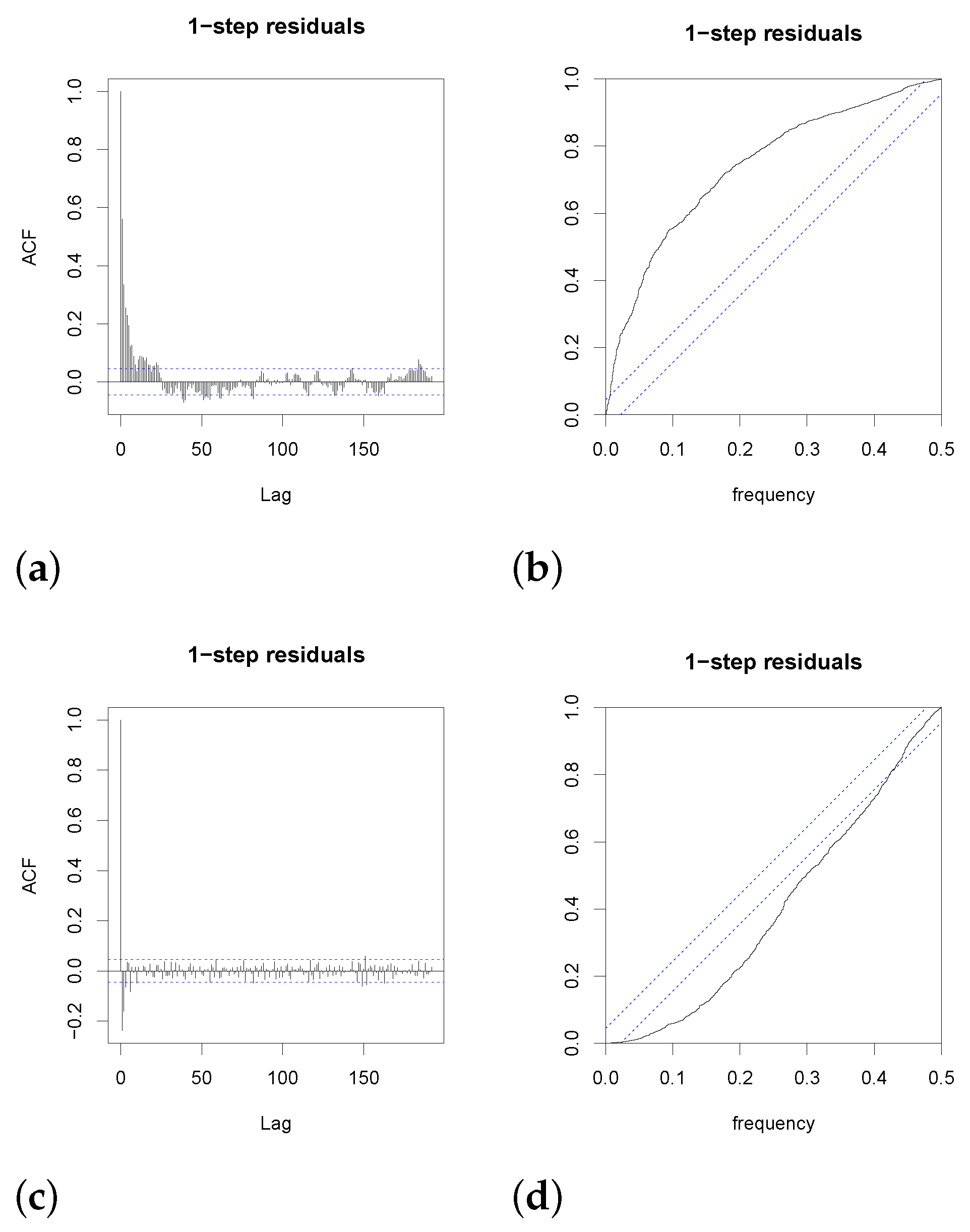
where t is the time variable; represents smooth functions as described in Section 5.4; , , , and are tensor product smooths; and the input variables are described in Table 1. The estimated parameters and function terms are reported in Table 2. Log-likelihood and RMSE values for the training and test data sets are presented in Table 3. Interestingly, the model maintains a similar RMSE for the test data set, which is promising for estimations and predictions outside the training data set. This is further validated in Figure 7, showing model predictions for the training and test data sets. Here, the predictions are very close to the observations, and the 95% confidence intervals can barely be seen due to the small span. Although showing good estimations and a low RMSE, the ACF (Figure 8) and cumulative periodogram (Figure 8) demonstrate patterns in the data that the model does not capture. Additionally, the model has 146 parameters (due to the smooth functions), which limits the explainability and possibility of extending the model to explain other end node behavior. For this reason, we need a model where the voltage drop for a section of the radial feeder can be separated/extracted.
6.2. Grey-Box Model
In the grey-box model, a lower model order was achieved with the following model structure:
where k are points in time, , of measurements; a, b, c, and d are parameters; represents a state for the voltage drop related to the resistance between and (), whereas represents a voltage drop state related to the reactance () along the same cables; is the discrete differential of the current at to the previous time step, i.e., (since only discrete measurements are available). Although inputs from the transformer devices could be used in the model structure, it had similar performance without these inputs. For instance, using the device at to model states for the voltage drop along the radial feeder from to and the neutral current voltage drop gave a log-likelihood of 1687 and RMSE of 0.100 and 0.108, for the training and test data sets, respectively. This is to be compared with the reported values in Table 3, keeping in mind that the model structure in the latter has 18 parameters, as opposed to nine parameters in the model in Equations (14) and (15). Obviously, the smaller model structure is preferred if its performance is comparable to or better than that of larger models. All other extensions, as described in Section 5.5, either proved to give insignificant parameters or produced similar or even worse performance in the predictions.
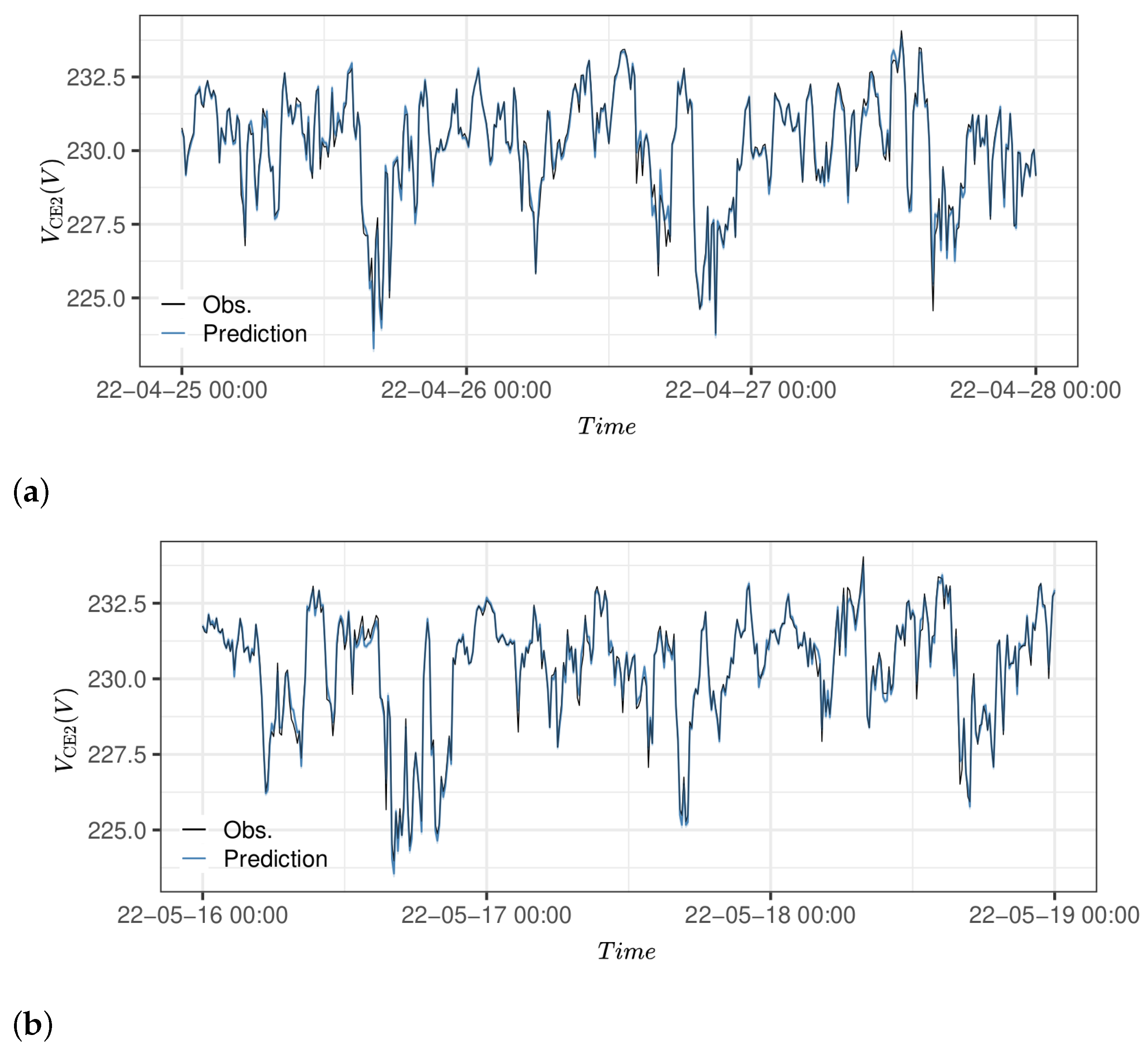
The estimated model parameters and standard errors are reported in Table 4. It can be seen that the p-values are very low and are more significant than the estimated parameters in the GAM model in general. Improvements compared to the GAM model are also seen in the residual ACF (Figure 8) and cumulative periodogram (Figure 8), indicating that there is almost no autocorrelation in the residuals. Thus, the model is better at capturing the existing patterns in the data. According to the cumulative periodogram, there are either higher frequencies left in the residuals or the model has a slight tendency towards overfitting. It should, however, be noted that the voltage tends to change quite rapidly, and higher-frequency patterns left in the residuals could be due to other load currents for which we do not have the measurements. Looking at the model performance on the training and test data sets in Figure 9, it can be concluded that although there is a slight deviation in the cumulative periodogram, the model performs exceptionally well even on the test data set.
The advantage of the grey-box model is the model structure, which offers more explainability compared to the GAM model. The grey-box model also has far fewer parameters than the GAM model. Furthermore, the estimated states of the grey-box model can be used to derive models for other end nodes in the radial network.
6.3. End Node Estimation
For the end node estimation model, a similar model evaluation process was performed as described in Section 6.1 and Section 6.2. Here, GAM models produced slightly better results compared to grey-box models for the end node estimations. At this stage in the workflow (see Figure 1), less explainability is required and accurate estimations and lower computation times are prioritized. Therefore, this section focuses on the results of the GAM models. The best results were acquired using the following model structure:
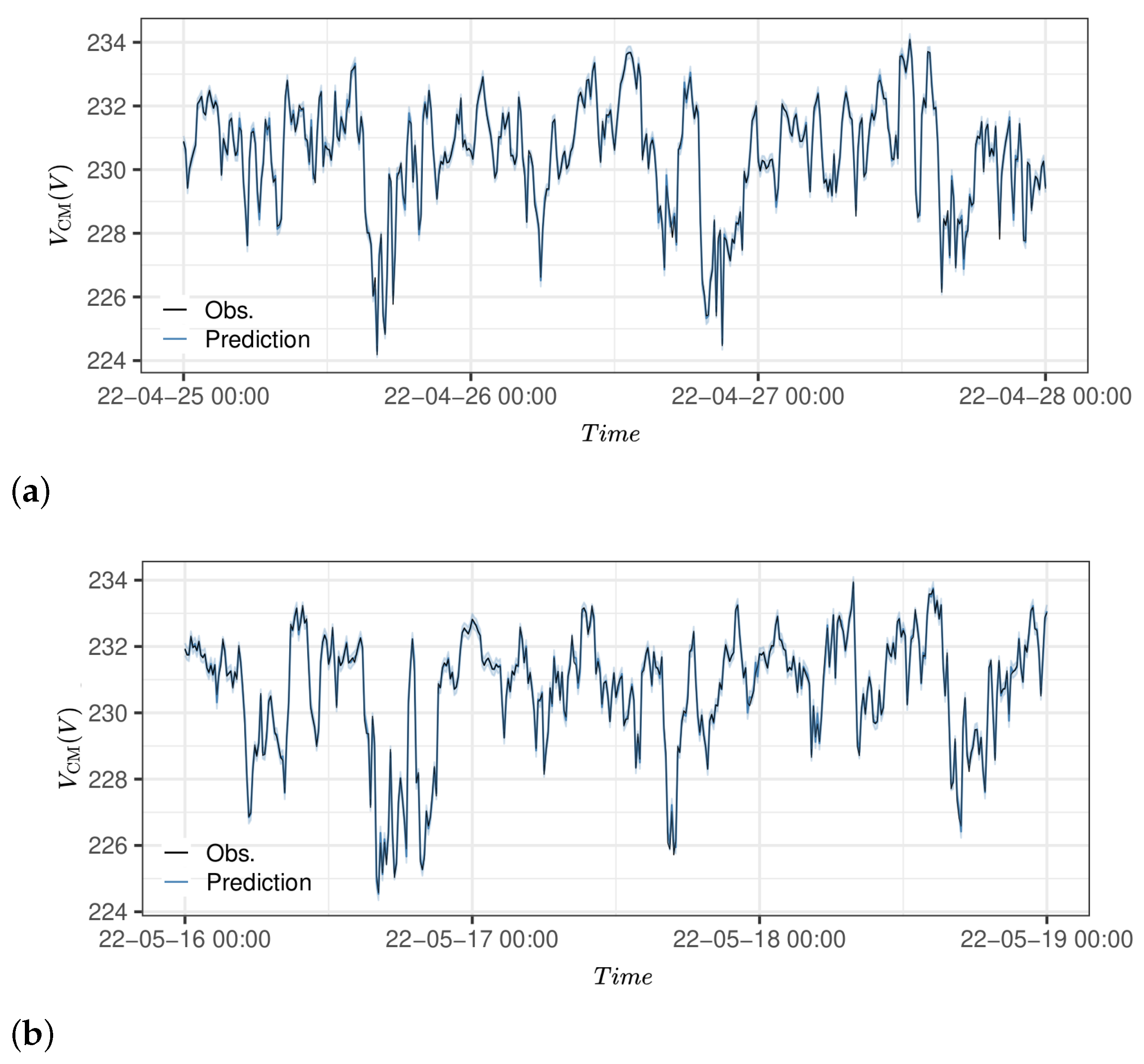
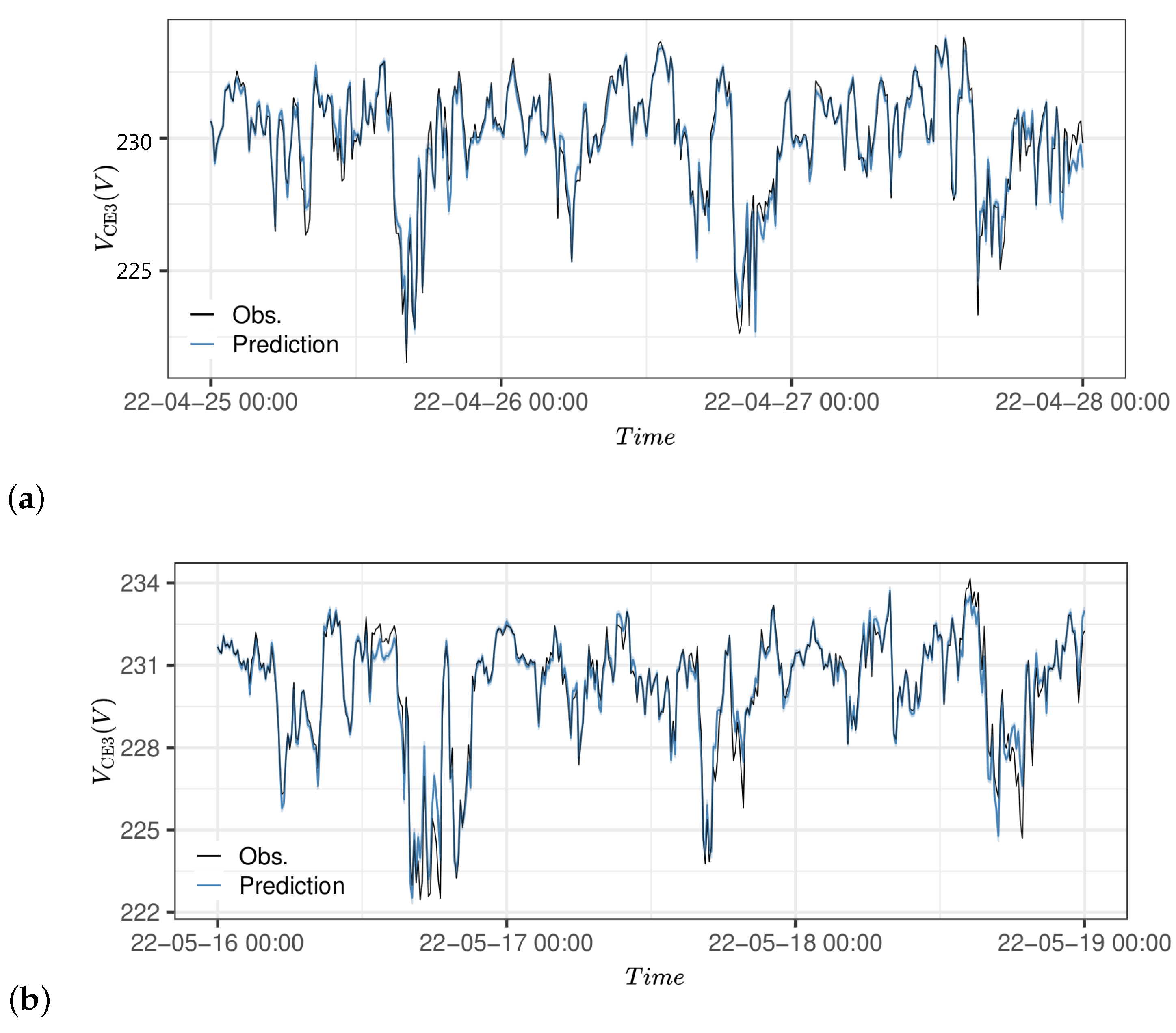
where is a seasonal spline for the daily variation using B-splines of degree 3 and 144 knots, and and are the estimated states of from the grey-box model. Incorporating , i.e., estimated from the grey-box model, demonstrated an insignificant impact on the model; hence, it was removed. Estimating the voltage at , , gave RMSE values of 0.22 V and 0.24 V for the training and test data sets, respectively, as well as the predictions in Figure 10. The voltage estimations, , at can be seen in Figure 11, for which the RMSE was 0.39 V and 0.49 V, respectively.
6.4. Analysis of Measurement Device Setup Configuration
To evaluate the impact of using the data from different nodes for end node voltage estimation, the proposed method is applied to the following cases.
- Case 1: Installing a measuring device at node and estimating the end node voltages at , , and .
- Case 2: Installing a measuring device at end node and estimating the voltage at and .
- Case 3: Installing two measuring devices at end nodes and and estimating the voltage at .
To model Case 1, Equation (16) is replaced by the following equation:
where represents the online measurement of the measuring device at . Case 2 is the proposed method in this paper. To implement Case 3, we should replace Equation (16) with the following equation:
where represents the online measurement of the measuring device at .
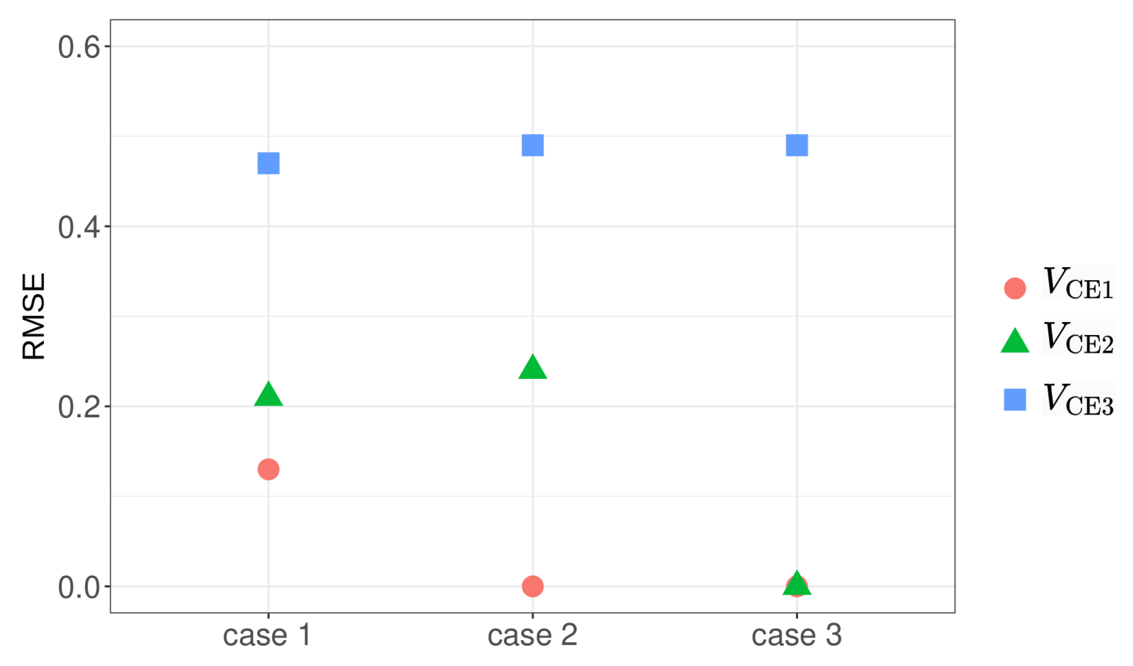
Simulation results of these cases are presented in Figure 12. As shown in Figure 12, Case 1 gives the best RMSE for voltage estimation in nodes and . This happens because, in this case, the estimation of the voltage in is replaced by online measurement, which reduces the error. However, the improvement in voltage estimation in comparison to other cases is not significant. Additionally, it does not provide the possibility of direct end node voltage measurement for any of the end nodes. In contrast with Case 1, Case 2 gives direct voltage measurement (RMSE = 0) in one end node due to installing the measuring device at end node , but, as mentioned before, the RMSEs for voltage estimation in other end nodes are slightly greater than in Case 1. Case 3 requires the installation of one more measuring device compared to Cases 1 and 2. However, as shown in Figure 12, adding a new device does not improve the RMSE of the estimation, although it gives the possibility of two direct measurements. Another case would involve installing devices at all end nodes to achieve direct measurement at , , and . As stated in Section 5.1, assuming that the DSO would have 1000 similar grids to the one presented in Figure 12, the latter would correspond to an installation setup with 22,000 devices, as opposed to 5000 devices for Cases 1 and 2. Overall, in Case 2, the number of required measuring devices is less than in Case 3, direct measurement possibility for one end node is obtained, and the estimation errors are close to those in Case 1. Thus, this is a good choice to install the measuring device and perform voltage estimation for all end nodes.
6.5. Application of the Proposed Method and Future Setup Extension
Following the results from the analysis in Section 6.4, placing the measuring device at produces better overall results. Furthermore, the models can be used in an online estimation or forecasting algorithm due to their fast computation times. The grey-box model parameters are optimized in 13.7 s, while the GAM models for voltages at and are optimized in 1.1 and 1.3 s, respectively, using an Intel core i7® 1.90 Ghz, with 16 GB RAM, running on Linux Pop!_OS version 21.10. It should be noted that for online operation, the computation times can be further improved—for instance, by choosing the previously estimated parameters as initial values. Similarly, the computation times for the grey-box modeling could be improved if the software CTSM-R was able to use several cores for parallel computation of the value of the likelihood function.
Comparing the computation times to other DSSE methods found in the literature, the proposed method performs well when considering the computation time of 0.79 h as in [28], and its result is similar to the computation time in [27] of 1 s. Furthermore, these computation times should be compared in the context of the prediction results. For instance, in [27], a mean average error of 0.3% was achieved, corresponding to 0.003 per unit (p.u.), and an RMSE of 0.59 V is reported in [25]. The RMSE for the end node estimations in this study ranges from 0.2 to 0.5 V (0.0008–0.002 p.u.) and the mid-node estimations are around 0.1 V (0.0004 p.u.).
Although the proposed models produce reasonable estimations, our models and experimental setup can be improved. There are two main action paths to improve the experimental setup:
- Improve measurements at , to measure all customers at the end node as well as the neutral conductor current;
- Improve measurements at , to measure all cables, including neutral conductors.
In the installation setup, the electrical data for two out of three customers at are measured. Since data from one customer are then missing, the model will not be able to capture the effects of their power consumption on the nodal voltage. While the overall daily pattern might be similar to that of the other customers, additional customer-specific patterns over the day will not be captured. This could also explain the potential presence of high-frequency residuals for the grey-box model in Figure 8, meaning that there are high-frequency patterns that the model might miss because the data are not available. This could be solved by measuring all customers at . Furthermore, the voltage drop along the neutral conductor was a significant input in the GAM model. However, we could only model the neutral conductor between and , since neutral phase data were only available at . Using inputs from only provided the best results from the grey-box model and, therefore, the impact of the neutral conductor voltage drop could not be explored. In a future installation setup, measurements for the neutral conductor should be provided for all devices. Unpredicted harmonics and voltage unbalance could result in neutral conductor currents affecting the line-to-ground voltage drop and thereby the model output. It is further suggested to measure the current and voltage of all cables and the neutral conductor at , instead of measuring only the cable toward (see Figure 2). It would then be possible to use the measurements at to directly estimate the end node voltages with the GAM model. It should, however, be noted that the first improvement still has the advantage of knowing one end node’s voltage with very high certainty and better explainabilty in extending the model structure to other radial feeders. A good practice could be to install both setup improvements and evaluate which one provides better model performance during a longer period of time.
With the short computation time, the models are also suitable for daily updates (optimizing model parameters) using smart meter data. As the workflow in Figure 1 along with the final models suggest, only one device is required for real-time operation and monitoring, whereas the offline model parameter optimization could be done at a preferred frequency when entire data sets are collected.
7. Conclusions
In this work, a data-driven nodal voltage estimation method for the real-time monitoring of radial LV grids has been developed. The method uses input from only one device at the end of a feeder and is designed to provide phase voltages. Such estimations are useful for distribution system operation as these grids are typically characterized by low or zero observability in the presence of voltage and current unbalance. With increasing volatility in consumption and production patterns, grid parameters, e.g., voltage and current, will show volatile behavior, especially if implementing flexibility services at this topological level in the grid. Therefore, real-time observability is of increasing importance for DSOs to avoid system failure and replace grid equipment in time.
The presented workflow uses both grey-box and GAM modeling techniques. Both methods have been proven to give reasonable estimations on both the training data set (13 days) and the test data set (31 days), with RMSEs of 0.0004–0.002 per unit (p.u.) for the studied nodes (for comparison, the voltage stability limits are p.u.). The grey-box model provides explainability in describing the voltage drop along parts of a feeder, which could be used as input to the computationally lighter GAM model. The method also provides confidence intervals, which give the DSO the opportunity to apply risk-informed strategies.
The proposed method has a low computational burden, which makes it useful for online monitoring algorithms, as opposed to other techniques relying on large data flows and high-bandwidth communication infrastructures. The computational time for optimizing the grey-box model parameters was 13.7 s, while the time required to optimize the GAM models was less than 2 s for each model.
Furthermore, the method was derived using data from a real-world radial LV grid. Working with real-world data and data-driven methods, such as the methods described in this paper, jointly offers a considerable contribution toward the application of observability models in DSO grids, as it reflects the real system with unavoidable disturbances, not captured through simulations in ideal conditions.
Future Work
From analyzing and using the data in the model’s development, useful insights have been gained and a few improvements to the experimental setup can be suggested. The improvements involve more comprehensive measurements at the end node used for model building, as well as at the middle node (). It is suggested that both improvements are implemented and the resulting models evaluated to obtain better model performance, and it is recommended further to install the setup in different LV grids to evaluate the scalability of the method.
Author Contributions
Conceptualization, E.M.V.B., M.B., R.E., O.S., F.D. and H.M.; Methodology, E.M.V.B.; Formal analysis, E.M.V.B.; Investigation, E.M.V.B.; Writing—original draft, E.M.V.B. and M.B.; Writing—review & editing, R.E., O.S. and H.M.; Visualization, E.M.V.B.; Supervision, R.E., O.S. and H.M.; Project administration, E.M.V.B. All authors have read and agreed to the published version of the manuscript.
Funding
This work was supported by the Flexible Energy Denmark (FED) project funded by Innovation Fund Denmark under Grant No. 8090-00069B, and the ebalanceplus project funded by the European Union’s Horizon 2020 under the grant agreement number of 864283.
Acknowledgments
The authors would like to thank Claus Schack Urup, TREFOR, for the technical support and for providing the data for this study.
Conflicts of Interest
The authors declare no conflict of interest.
References
- D’Ettorre, F.; Banaei, M.; Ebrahimy, R.; Pourmousavi, S.A.; Blomgren, E.; Kowalski, J.; Bohdanowicz, Z.; Łopaciuk-Gonczaryk, B.; Biele, C.; Madsen, H. Exploiting demand-side flexibility: State-of-the-art, open issues and social perspective. Renew. Sustain. Energy Rev. 2022, 165, 112605. [Google Scholar] [CrossRef]
- Táczi, I.; Sinkovics, B.; Vokony, I.; Hartmann, B. The challenges of low voltage distribution system state estimation—An application oriented review. Energies 2021, 14, 5363. [Google Scholar] [CrossRef]
- Dehghanpour, K.; Wang, Z.; Wang, J.; Yuan, Y.; Bu, F. A survey on state estimation techniques and challenges in smart distribution systems. IEEE Trans. Smart Grid 2019, 10, 2312–2322. [Google Scholar] [CrossRef]
- Wang, H.; Schulz, N.N. A Revised Branch Current-Based Distribution System State Estimation Algorithm and Meter Placement Impact. IEEE Trans. Power Syst. 2004, 19, 207–213. [Google Scholar] [CrossRef]
- Pau, M.; Pegoraro, P.A.; Sulis, S. Efficient branch-current-based distribution system state estimation including synchronized measurements. IEEE Trans. Instrum. Meas. 2013, 62, 2419–2429. [Google Scholar] [CrossRef]
- Baran, M.E.; Jung, J.; McDermott, T.E. Including voltage measurements in branch current state estimation for distribution systems. In Proceedings of the 2009 IEEE Power and Energy Society General Meeting, PES ’09, Calgary, AB, Canada, 26–30 July 2009. [Google Scholar] [CrossRef]
- Monticelli, A. State Estimation in Electric Power Systems: A Generalized Approach; Springer: New York, NY, USA, 1999; Volume 7. [Google Scholar]
- Lin, W.M.; Teng, J.H. State Estimation for Distribution Systems with Zero-Injection Constraints. In IEEE Transactions on Power Systems; IEEE: Piscataway, NJ, USA, 1996. [Google Scholar]
- Chen, Q.; Kaleshi, D.; Fan, Z.; Armour, S. Impact of Smart Metering Data Aggregation on Distribution System State Estimation. IEEE Trans. Ind. Inform. 2016, 12, 1426–1437. [Google Scholar] [CrossRef]
- Nie, Y.; Chung, C.Y.; Xu, N.Z. System State Estimation Considering EV Penetration with Unknown Behavior Using Quasi-Newton Method. IEEE Trans. Power Syst. 2016, 31, 4605–4615. [Google Scholar] [CrossRef]
- Yao, Y.; Liu, X.; Zhao, D.; Li, Z. Distribution System State Estimation: A Semidefinite Programming Approach. IEEE Trans. Smart Grid 2019, 10, 4369–4378. [Google Scholar] [CrossRef]
- Zhu, H.; Giannakis, G.B. Power system nonlinear state estimation using distributed semidefinite programming. IEEE J. Sel. Top. Signal Process. 2014, 8, 1039–1050. [Google Scholar] [CrossRef]
- Wu, J.; He, Y.; Jenkins, N. A robust state estimator for medium voltage distribution networks. IEEE Trans. Power Syst. 2013, 28, 1008–1016. [Google Scholar] [CrossRef]
- Liu, B.; Wu, H.; Zhang, Y.; Yang, R.; Bernstein, A. Robust Matrix Completion State Estimation in Distribution Systems. In Proceedings of the 2019 IEEE Power & Energy Society General Meeting (PESGM), Piscataway, NJ, USA, 4–8 August 2019. [Google Scholar]
- Lin, C.; Wu, W.; Guo, Y. Decentralized Robust State Estimation of Active Distribution Grids Incorporating Microgrids Based on PMU Measurements. IEEE Trans. Smart Grid 2020, 11, 810–820. [Google Scholar] [CrossRef]
- Dahale, S.; Karimi, H.S.; Lai, K.; Natarajan, B. Sparsity based approaches for distribution grid state estimation—A comparative study. IEEE Access 2020, 8, 198317–198327. [Google Scholar] [CrossRef]
- Raghuvamsi, Y.; Teeparthi, K. Detection and reconstruction of measurements against false data injection and DoS attacks in distribution system state estimation: A deep learning approach. Meas. J. Int. Meas. Confed. 2023, 210, 112565. [Google Scholar] [CrossRef]
- Zamzam, A.S.; Fu, X.; Sidiropoulos, N.D. Data-Driven Learning-Based Optimization for Distribution System State Estimation. IEEE Trans. Power Syst. 2019, 34, 4796–4805. [Google Scholar] [CrossRef]
- Dehghanpour, K.; Yuan, Y.; Wang, Z.; Bu, F. A Game-Theoretic Data-Driven Approach for Pseudo-Measurement Generation in Distribution System State Estimation. IEEE Trans. Smart Grid 2019, 10, 5942–5951. [Google Scholar] [CrossRef]
- Kim, D.; Dolot, J.M.; Song, H. Distribution System State Estimation Using Model-Optimized Neural Networks. Appl. Sci. 2022, 12, 2073. [Google Scholar] [CrossRef]
- Zamzam, A.S.; Sidiropoulos, N.D. Physics-Aware Neural Networks for Distribution System State Estimation. IEEE Trans. Power Syst. 2019, 35, 4347–4356. [Google Scholar] [CrossRef]
- Menke, J.H.; Bornhorst, N.; Braun, M. Distribution system monitoring for smart power grids with distributed generation using artificial neural networks. Int. J. Electr. Power Energy Syst. 2019, 113, 472–480. [Google Scholar] [CrossRef]
- Weng, Y.; Negi, R.; Faloutsos, C.; Ilic, M.D. Robust Data-Driven State Estimation for Smart Grid. IEEE Trans. Smart Grid 2017, 8, 1956–1967. [Google Scholar] [CrossRef]
- Anubi, O.M.; Konstantinou, C. Enhanced resilient state estimation using data-driven auxiliary models. IEEE Trans. Ind. Inform. 2020, 16, 639–647. [Google Scholar] [CrossRef]
- Pertl, M.; Douglass, P.J.; Heussen, K.; Kok, K. Validation of a robust neural real-time voltage estimator for active distribution grids on field data. Electr. Power Syst. Res. 2018, 154, 182–192. [Google Scholar] [CrossRef]
- Procopiou, A.T.; Ochoa, L.F. Voltage Control in PV-Rich LV Networks Without Remote Monitoring. IEEE Trans. Power Syst. 2017, 32, 1224–1236. [Google Scholar] [CrossRef]
- Mokaribolhassan, A.; Nourbakhsh, G.; Ledwich, G.; Arefi, A.; Shafiei, M. Distribution System State Estimation Using PV Separation Strategy in LV Feeders with High Levels of Unmonitored PV Generation. IEEE Syst. J. 2023, 17, 684–695. [Google Scholar] [CrossRef]
- Rigoni, V.; Soroudi, A.; Keane, A. Use of fitted polynomials for the decentralised estimation of network variables in unbalanced radial LV feeders. IET Gener. Transm. Distrib. 2020, 14, 2368–2377. [Google Scholar] [CrossRef]
- IEEE Std. 141-1993; Recommended Practice for Electric Power Distribution for Industrial Plants. The Institute of Electrical and Electronics Engineers, Inc.: New York, NY, USA, 1994. [CrossRef]
- Degroote, L.; Renders, B.; Meersman, B.; Vandevelde, L. Neutral-point shifting and voltage unbalance due to single-phase DG units in low voltage distribution networks. In Proceedings of the 2009 IEEE Bucharest PowerTech: Innovative Ideas Toward the Electrical Grid of the Future, Bucharest, Romania, 28 June–2 July 2009; pp. 1–8. [Google Scholar] [CrossRef]
- Jung, T.H.; Gwon, G.H.; Kim, C.H.; Han, J.; Oh, Y.S.; Noh, C.H. Voltage Regulation Method for Voltage Drop Compensation and Unbalance Reduction in Bipolar Low-Voltage DC Distribution System. IEEE Trans. Power Deliv. 2018, 33, 141–149. [Google Scholar] [CrossRef]
- Pandian, S.S. Various considerations for estimating steady-state voltage drop in low voltage AC power distribution systems. In Proceedings of the Conference Record—Industrial and Commercial Power Systems Technical Conference, Detroit, MI, USA, 30 April–3 May 2006. [Google Scholar] [CrossRef]
- Wood, S.N. Generalized Additive Models: An Introduction with R, 2nd ed.; CRC Press: Boca Raton, FL, USA, 2017. [Google Scholar] [CrossRef]
- Wood, S.N. Fast stable restricted maximum likelihood and marginal likelihood estimation of semiparametric generalized linear models. J. R. Stat. Soc. B 2011, 73, 3–36. [Google Scholar] [CrossRef]
- Wood, S.; Pya, N.; Säfken, B. Smoothing parameter and model selection for general smooth models (with discussion). J. Am. Stat. Assoc. 2016, 111, 1548–1575. [Google Scholar] [CrossRef]
- Wood, S.N. Stable and efficient multiple smoothing parameter estimation for generalized additive models. J. Am. Stat. Assoc. 2004, 99, 673–686. [Google Scholar] [CrossRef]
- Wood, S.N. Thin-plate regression splines. J. R. Stat. Soc. B 2003, 65, 95–114. [Google Scholar] [CrossRef]
- Bacher, P.; Madsen, H. Identifying suitable models for the heat dynamics of buildings. Energy Build. 2011, 43, 1511–1522. [Google Scholar] [CrossRef]
- Stentoft, P.A.; Munk-Nielsen, T.; Vezzaro, L.; Stentoft, P.A.; Madsen, H.; Møller, J.K.; Vezzaro, L.; Mikkelsen, P.S. Towards model predictive control: Online predictions of ammonium and nitrate removal by using a stochastic ASM. Water Sci. Technol. 2019, 79, 51–62. [Google Scholar] [CrossRef] [PubMed]
- Juhl, R.; Møller, J.K.; Madsen, H. Ctsmr—Continuous Time Stochastic Modeling in R. arXiv 2016, arXiv:1606.00242. [Google Scholar]
- Kristensen, N.R.; Madsen, H.; Jørgensen, S.B. Parameter estimation in stochastic grey-box models. Automatica 2004, 40, 225–237. [Google Scholar] [CrossRef]
- Juhl, R.; Møller, J.K.; Jørgensen, J.B.; Madsen, H. Modeling and Prediction Using Stochastic Differential Equations. In Prediction Methods for Blood Glucose Concentration; Springer: Berlin/Heidelberg, Germany, 2016; pp. 183–209. [Google Scholar] [CrossRef]
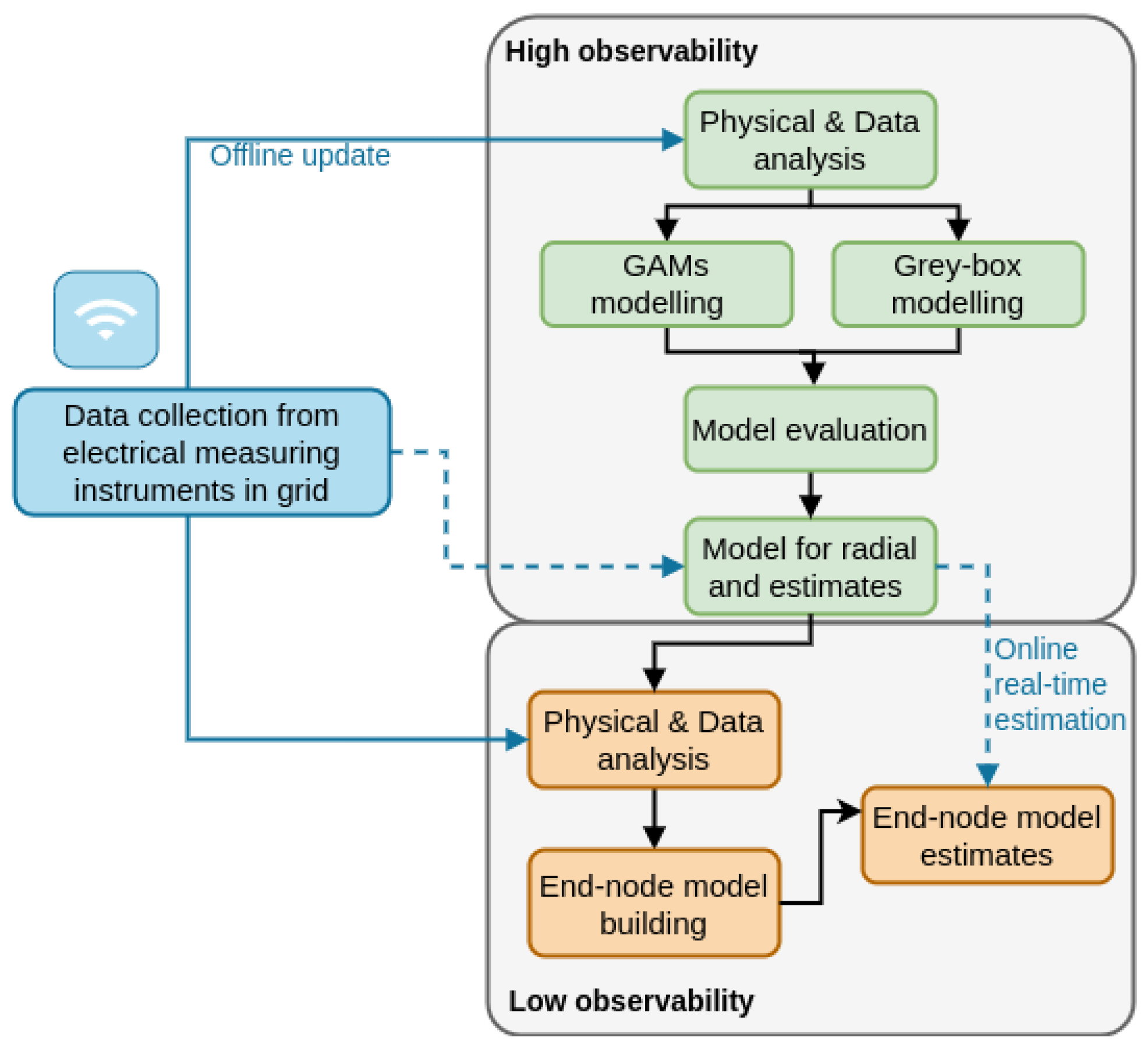
Figure 1.
Workflow for the model selection process. Solid arrows represent the offline model selection approach using data collected from the power grid. Dotted arrows represent how the model would operate in real time using measurements and model estimates from a radial with high observability to estimate end nodes with lower observability.

Figure 2.
Grid topology and installation of devices (blue dotted circles). The naming of the devices is constructed from the letter of the feeder (i.e., A, B, C, D, and F), subscript M indicates that it is a middle node, and subscript E indicates an end node. and represent the two devices installed at the transformer. It is also indicated whether the device measures both voltage and current or only voltage [V]. Squares represent customers in the grid.

Figure 3.
Phase L3 voltage measurements of all devices on feeder C. is the voltage at the transformer (device ) and , , , and are voltages at the corresponding devices on the feeder.
Figure 3.
Phase L3 voltage measurements of all devices on feeder C. is the voltage at the transformer (device ) and , , , and are voltages at the corresponding devices on the feeder.

Figure 4.
Scatter plots, data density, and correlation for voltages and neutral current, for all devices on feeder C (i.e., , , , , and ) using a time resolution of 10 min. “***” indicates a p-value < 0.001, “.” indicate a p-value < 0.10.
Figure 4.
Scatter plots, data density, and correlation for voltages and neutral current, for all devices on feeder C (i.e., , , , , and ) using a time resolution of 10 min. “***” indicates a p-value < 0.001, “.” indicate a p-value < 0.10.

Figure 5.
Scatter plots, data density, and correlation for voltages and input variables, using a time resolution of 10 min. “***” indicates a p-value < 0.001, “**” indicate a p-value < 0.01, “*” indicate a p-value < 0.05, “.” indicate a p-value < 0.10.
Figure 5.
Scatter plots, data density, and correlation for voltages and input variables, using a time resolution of 10 min. “***” indicates a p-value < 0.001, “**” indicate a p-value < 0.01, “*” indicate a p-value < 0.05, “.” indicate a p-value < 0.10.

Figure 6.
Phase L3 voltage time series for device filtered to time resolutions 1 min, 5 min, 10 min, and 15 min.
Figure 6.
Phase L3 voltage time series for device filtered to time resolutions 1 min, 5 min, 10 min, and 15 min.

Figure 7.
GAM model state estimates on training (a) and test (b) data sets for three days, respectively. The black and blue lines represent the observations and the model predictions, respectively. There is also a 95% confidence interval indicated by the blue area, but it is visually difficult to see in the graph due to the low standard deviation in the model.

Figure 8.
Residual ACFs and cumulative periodograms, for the GAM model in (a,b) and for the grey-box model in (c,d). Blue horizontal and diagonal lines indicate a 95% confidence interval.
Figure 8.
Residual ACFs and cumulative periodograms, for the GAM model in (a,b) and for the grey-box model in (c,d). Blue horizontal and diagonal lines indicate a 95% confidence interval.

Figure 9.
Grey-box model estimations on the training, (a) and test (b) data sets for three days, respectively. The black line represents the observations, and the blue line shows the model predictions. A blue area also indicates a 95% confidence interval, but it is visually difficult to see in the graph due to the low standard deviation in the model.

Figure 10.
GAM model estimations on the training (a) and test (b) data sets for for three days, respectively. The black line represents the observations and the blue line represents the model predictions. There is also a 95% confidence interval indicated by a blue area.
Figure 10.
GAM model estimations on the training (a) and test (b) data sets for for three days, respectively. The black line represents the observations and the blue line represents the model predictions. There is also a 95% confidence interval indicated by a blue area.

Figure 11.
GAM model estimations on the training (a) and test (b) data sets for zooming in on three days, respectively. The black line represents the observations and the blue line represents the model predictions. There is also a 95% confidence interval indicated by a blue area.
Figure 11.
GAM model estimations on the training (a) and test (b) data sets for zooming in on three days, respectively. The black line represents the observations and the blue line represents the model predictions. There is also a 95% confidence interval indicated by a blue area.

Figure 12.
RMSE for voltage estimations at end nodes (red circle), (green triangle), and (blue square). Case 1 corresponds to installation of a measuring device at node and estimating the end node voltages at , , and ; Case 2 corresponds to installation of a measuring device at end node and estimating voltage at and ; Case 3 corresponds to installation of two measuring devices at end nodes and and estimating the voltage at .


Table 1.
Measured input variables used in the model selection process. All electrical measurements from the experimental setup are per phase, and their placements in the LV grid are seen in Figure 2.
Table 1.
Measured input variables used in the model selection process. All electrical measurements from the experimental setup are per phase, and their placements in the LV grid are seen in Figure 2.
| Variable | Notation | Unit |
|---|---|---|
| voltage at | V | |
| voltage at | V | |
| voltage at | V | |
| voltage at | V | |
| voltage at | V | |
| current at | A | |
| power factor at | - | |
| neutral conductor current at | A | |
| neutral conductor power factor at | - | |
| neutral conductor current at | A | |
| neutral conductor power factor at | - | |
| current at | A | |
| power factor at | - | |
| current at | A | |
| power factor at | - | |
| solar radiation (from DMI) | W/m | |
| ambient temperature (from DMI) | °C |
Table 2.
Estimated parameters and function terms in Equation (12), as well as corresponding p-values.
Table 2.
Estimated parameters and function terms in Equation (12), as well as corresponding p-values.
| Parameter/Term | Estimated | p-Value |
|---|---|---|
| Intercept | < | |
| < | ||
| < | ||
| < |
Table 3.
Comparison of log-likelihood between the GAM and grey-box models, as well as RMSEs of the training and test data sets.
Table 3.
Comparison of log-likelihood between the GAM and grey-box models, as well as RMSEs of the training and test data sets.
| GAM | Grey-Box | |
|---|---|---|
| Log likelihood | 1678 | 1685 |
| RMSE training data set | 0.099 | 0.100 |
| RMSE test data set | 0.109 | 0.107 |
Disclaimer/Publisher’s Note: The statements, opinions and data contained in all publications are solely those of the individual author(s) and contributor(s) and not of MDPI and/or the editor(s). MDPI and/or the editor(s) disclaim responsibility for any injury to people or property resulting from any ideas, methods, instructions or products referred to in the content. |
© 2023 by the authors. Licensee MDPI, Basel, Switzerland. This article is an open access article distributed under the terms and conditions of the Creative Commons Attribution (CC BY) license (https://creativecommons.org/licenses/by/4.0/).
Share and Cite
MDPI and ACS Style
Blomgren, E.M.V.; Banaei, M.; Ebrahimy, R.; Samuelsson, O.; D’Ettorre, F.; Madsen, H. Intensive Data-Driven Model for Real-Time Observability in Low-Voltage Radial DSO Grids. Energies 2023, 16, 4366. https://doi.org/10.3390/en16114366
AMA Style
Blomgren EMV, Banaei M, Ebrahimy R, Samuelsson O, D’Ettorre F, Madsen H. Intensive Data-Driven Model for Real-Time Observability in Low-Voltage Radial DSO Grids. Energies. 2023; 16(11):4366. https://doi.org/10.3390/en16114366
Chicago/Turabian StyleBlomgren, Emma M. V., Mohsen Banaei, Razgar Ebrahimy, Olof Samuelsson, Francesco D’Ettorre, and Henrik Madsen. 2023. "Intensive Data-Driven Model for Real-Time Observability in Low-Voltage Radial DSO Grids" Energies 16, no. 11: 4366. https://doi.org/10.3390/en16114366
Note that from the first issue of 2016, this journal uses article numbers instead of page numbers. See further details here.