Design and Control of a Three-Axis Motion Servo Control System Based on a CAN Bus

Abstract

The paper presents a DSP-based design and control of a three-axis servo motion system that effectively divides control tasks between the master control terminal and four slave drives. The proposed architecture enhances the immediacy of platform positioning and the integration between software and hardware. The paper utilizes a high-accuracy encoder as a reference value for accuracy improvement and integrates firmware via the proposed embedded execution program, thereby reducing the accuracy error of the low-accuracy encoder. The main control core employs a digital signal processor (DSP) for input and output signal reading and writing, digital communication interface processing, and user interface. The slave controller utilizes four digital signal processors to accomplish servo position control in a digital way. The paper employs encoder calibration technology to upgrade the positioning accuracy of the surge axis. Finally, the paper validates the correctness and feasibility of the proposed method through experimental results from a set of adjustable experimental platforms of linear motion stroke and rotary motion stroke. In summary, the paper underscores the integration of hardware and software to attain high-precision and dependable control of the motion system.

1. Introduction

Nowadays, there is great demand for gantry machines with functionality, a wide range of applications, low production costs, and high applicability. These machines provide precise positioning operations and flexible processing characteristics to perform routine production processes [1]. The use of servo motion control improves the precision of manufactured products because the alternative to the servo drive can be a system based on a servo motor. When a poor angle signal occurs, it can seriously affect the operation of the machine. Therefore, multi-axis servo drives need to have high dynamic characteristics and positioning accuracy [2]. In [3], static friction dynamics and its compensation in the field of motion control were analyzed. However, the discontinuous dynamics of static friction, known as stick–slip, make it difficult to deal with. The dual drive system [4] is a newly designed transmission mechanism applied on the Internet using the extension of the real-time network protocol UDP. In [5], Ferrel showed that kinesthetically coupled remote manipulation can become unstable due to time delays [6]. If the time delay is constant, a Smith compensator may be a good solution [7]. Anderson et al. introduced an architecture with an infinite delay stability margin [8]. However, time delays in networks always vary due to unpredictable factors. To overcome this, Leung et al. applied a technique that models time-delayed jitters as disturbances based on robust control theory [9]. This is an effective way to deal with the randomness of network load but still requires an estimate of worst-case latency in order to reduce the problem of transmission delay, improve the dynamic characteristics of the servo, and improve the quality of platform transmission. The ability to transfer data over the bus does not require human-to-human or human-to-machine interaction.

Currently popular bus methods on the market are RS485, RS422 RS232, and the controller area network (CAN). While RS485, RS422, RS232, and other serial bus slave structures exhibit poor real-time reliability, CAN is a serial distributed control network with good bus utilization, a fast transmission rate (maximum 1 Mbit/s), low cost, and reliably good real-time performance. CAN also supports a distributed control network, widely used in robot control, industrial automation, car, aerospace, and other fields, making it one of the most widely used field buses. The CAN bus was proposed by the German company BOSCH in the early 1980s [10]. At the time, it was to solve the issues with the serial communication technology used by the company for data exchange between the control of the car and the instrumentation in the car. Compared with other buses, the advantages of CAN bus are that it can be used in multi-host mode, can achieve point-to-point or point-to-multipoint propagation mode, can reach a transmission rate of 1 Mbps, and has high system scalability, as well as the fact that CRC error detection can verify whether data are successfully sent, and the node with higher priority can transmit data first [11]. In [12], research on network-based control was found to be a promising solution for dealing with complex problems in systems with many sensors and actuators. Networked control systems need to avoid delays and packet loss caused by the network [13]. For networked control systems, a controller area network (CAN) is widely used in the automotive industry. According to this, the delay in CAN is divided into four types: frame delay, software delay, CAN controller delay, and user access delay [14].

Stewart platforms are used for most types of flight training [15,16]. The prototype of the Stewart platform was designed by V. E. Gough in 1956 and was built for work-related purposes [17]. Afterwards, it was improved by D. Stewart in 1965, and a parallel six-axis robot was proposed for the first time in 1965, which was later widely called the Stewart platform [18]. The Stewart platform is used in flight simulator training, so the Stewart platform was used as the standard body of the flight simulator in the early days. Therefore, the prospect of parallel platforms has attracted widespread attention from many scholars, and numerous related studies have been carried out. Research since 2010 has generally involved methods for controlling parallel architectures, such as predictive control [19,20,21] and artificial neural network control [22]. More recent research has focused on numerical solutions. For example, the motion spatial extent of the upper platform and the center of the platform can be obtained via kinematics [23]. In addition, [24] proposed that the angle update command problem of the six motors caused by multi-threading can be solved via a real-time algorithm. The characteristics of the proposed method can reduce the running time and increase the calculation speed so that the update command of the motor angle of the motion platform can be more accurately updated to six servo drives at once. Other research has applied real-life dynamic proprioception, creating the same sensation of motion as in a real-life vehicle. When the motion state of the platform is the same or similar to that of a real vehicle, it means that the motion prompt effect is close to reality [25,26]. Therefore, the movement of the simulator can be specially aimed at the perception of speed and acceleration of the human sensory system so as to realize a feeling of movement that is as realistic as possible.

This paper presents a comprehensive study on a three-degree-of-freedom platform that offers a new approach to motion control. The platform is designed with a digital control system that provides a stable and versatile mechanism design, which allows for continuous rotation and long-distance stroke. The pitch and yaw axes can rotate a full 360 degrees, while the surge axis employs a moving column gantry structure driven by both sides to enhance the dynamic motion effect of linear acceleration. The proposed embedded execution program is employed to improve positioning accuracy, which is critical for achieving high-precision motion control. This study provides innovative ideas in mechanism design, kinematics, embedded executive programs, and control systems, which have not been previously proposed in the literature [1,2,3,4,5,6,7,8,9,10,11,12,13,14,15,16,17,18,19,20,21,22,23,24,25,26,27]. These contributions are significant and demonstrate the potential of digital control systems for motion control applications. Additionally, sensors are installed on the platform to monitor and track the performance evaluation of axis motion, enabling researchers to study the platform’s behavior and optimize its control algorithms. The system’s core is based on DSP, which enables servo control and motion control. The three-axis motion control is achieved by reading and receiving instructions via the CAN bus communication port, which provides a reliable and efficient method of data transmission. Overall, this paper provides a deep understanding of the platform’s performance, which is essential for researchers or engineers interested in motion control applications.

2. The Motion Platform Control

2.1. System Overview

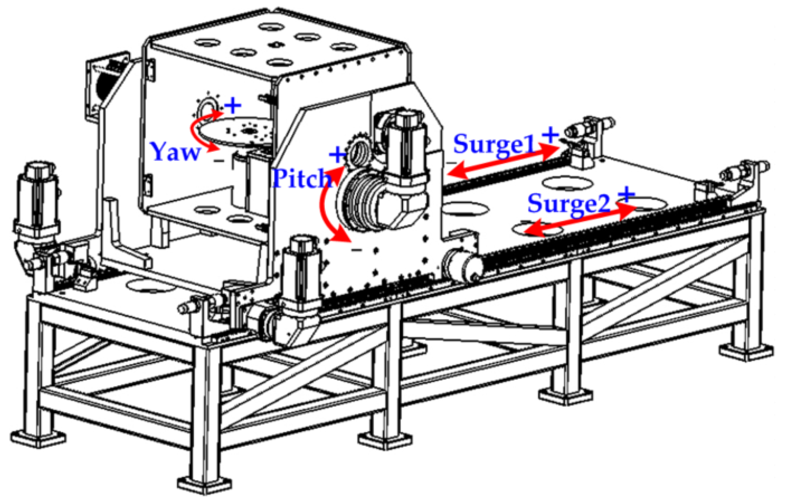
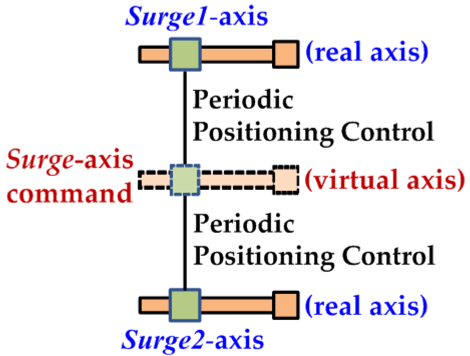
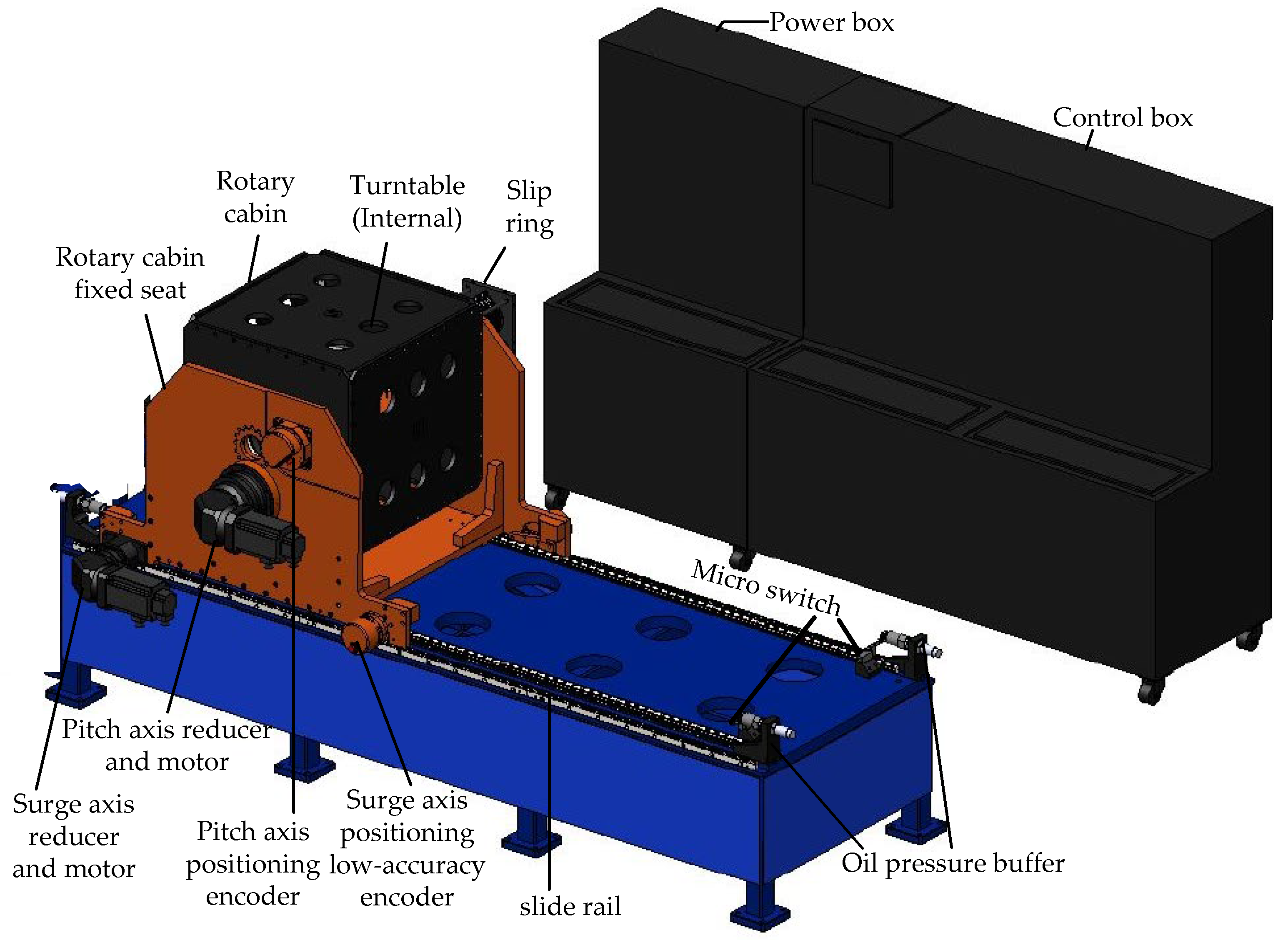
The platform mainly consists of a rotary cabin, a slip ring, four reducers, four motors, two positioning encoders, two slide rails, two racks, four oil pressure buffers, and four micro switches, as depicted in Figure 1. The 3-DOF motion is actuated by 4 electric motors, i.e., a linear motion (surge axis) driven by bilateral electric motors, with 2 rotary motions (pitch axis and yaw axis) respectively provided by 2 electric motors to the rotary cabin and the rotary table to achieve the rolling effect. The DSP controller uses the virtual axis command, moves along with the surge1 axis and the surge2 axis every 1 ms cycle time, and controls the real axis of surge1 and surge2 to execute motion control with the virtual axis as the command. This relationship is shown in Figure 2.

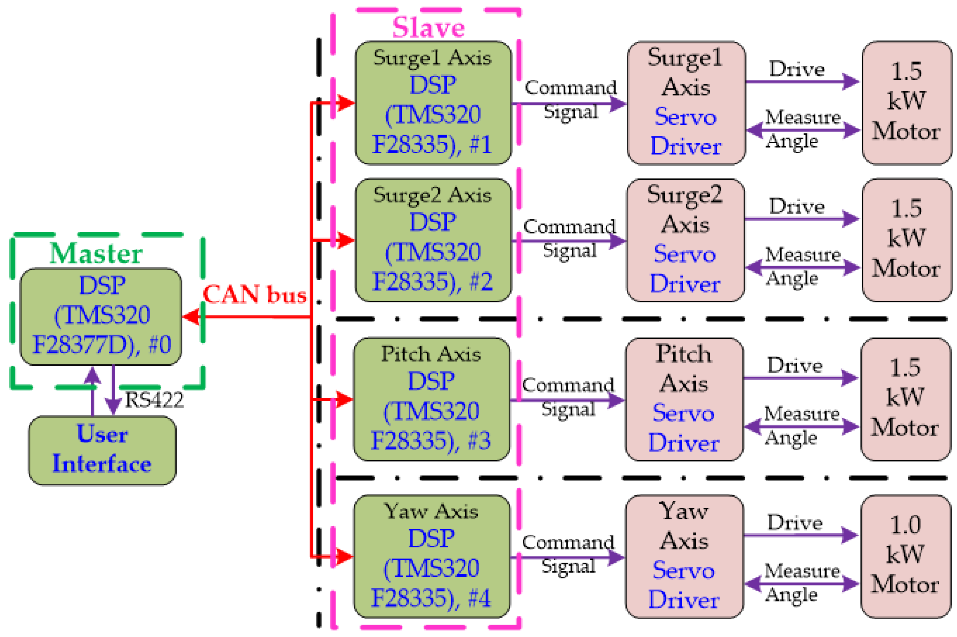
The control system uses 1 digital signal processor (DSP) (#0) to perform digital control as the master control terminal and 4 DSPs (#1~#4) to perform digital control as the slave control. Motion control is performed using 5 DSP controllers. The servo motors use four DSPs as the controlled object, accept the control signal sent by the upper layer through the CAN bus, execute the corresponding command, and send the feedback result to the master control terminal in real time. The CAN bus and DSPs execution data are connected in series. Therefore, in addition to the CAN bus communication, the DSP (#0) can also receive the other DSPs data and connect the two lines of CAN_H and CAN_L to the surge1 and surge2 axes, pitch axis, and yaw axis, as shown in Figure 3. The user interface displays the current status of the equipment, the attitude of each axis, the speed, the torque, and other information.

As shown in the relationship in Figure 3, the master controller (#0) reads the angles of the real axes of surge1 and surge2 and calculates the center position of the real axis of the surge.

$$\mathrm{T}\mathrm{h}\mathrm{e}\mathrm{t}{\mathrm{a}}_{\mathrm{surge}}=\frac{\mathrm{T}\mathrm{h}\mathrm{e}\mathrm{t}{\mathrm{a}}_{\mathrm{surge}1}+\mathrm{T}\mathrm{h}\mathrm{e}\mathrm{t}{\mathrm{a}}_{\mathrm{surge}2}}{2}$$

(1)

Therefore, the rotation angle of surge1 and surge2 can be controlled by the virtual axis command to move to the center of the two axes. If it is greater than the set 0.05°, the software will detect whether the threshold is exceeded, and surge1 and surge2 will stop running immediately. The simultaneous movement and stop of each axis use the commands of maximum acceleration, maximum deceleration, and maximum speed to obtain the acceleration, deceleration, and instantaneous speed commands of each axis. Taking the number of movements of the surge axis, pitch axis, and yaw axis trajectory as the motion reference, the speed command, acceleration command, and deceleration command can be expressed as

$${\mathrm{Velocity}}_{\mathrm{i}}=\frac{\left({\mathrm{Velocity}}_{\max }\right)\cdot \left({\mathrm{Displacement}}_{\mathrm{i}}\right)}{\left(\mathrm{Displacement}\right)}, \mathrm{i}=\mathrm{surge},\mathrm{pitch},\mathrm{yaw}$$

(2)

$${\mathrm{Acceleration}}_{\mathrm{i}}=\frac{\left({\mathrm{Acceleration}}_{\max }\right)\cdot \left({\mathrm{Displacement}}_{\mathrm{i}}\right)}{\left(\mathrm{Displacement}\right)}, \mathrm{i}=\mathrm{surge},\mathrm{pitch},\mathrm{yaw}$$

(3)

$${\mathrm{Deceleration}}_{\mathrm{i}}=\frac{\left({\mathrm{Deceleration}}_{\max }\right)\cdot \left({\mathrm{Displacement}}_{\mathrm{i}}\right)}{\left(\mathrm{Displacement}\right)}, \mathrm{i}=\mathrm{surge},\mathrm{pitch},\mathrm{yaw}$$

(4)

and

$$\mathrm{Displacement}=\sqrt{{\displaystyle \sum _{\mathrm{i}=\mathrm{surge},\mathrm{pitch},\mathrm{yaw}}{\mathrm{Displacement}}_{\mathrm{i}}^2}}$$

(5)

Thus, from Equations (1)–(5), the relational expressions of speed, acceleration, and deceleration required for multi-axis drive can be obtained.

2.2. Closed-Loop Control Strategy

Several researchers have proposed different ways to tune the parameters of the plant to achieve the required performance of a closed-loop control system. Recently, several papers have proposed controllers dealing with uncertainty in vehicle systems. For example, Shukla et al. [28] designed a robust adaptive controller for the steer-by-wire system. Yadav et al. [29] studied an adaptive sliding mode controller for autonomous vehicle platoon, with their simulation and experimental studies showing that a realistic scenario representing repeated narrow and wide paths for robots leads to significant performance loss for non-switched controllers. Rayguru et al. [30] studied an extended high-gain observer. Accurate estimation of uncertain dynamics terms for compensation purposes was incorporated into an output–feedback controller for a proposed reconfigurable road-sweeping wheeled mobile robot.

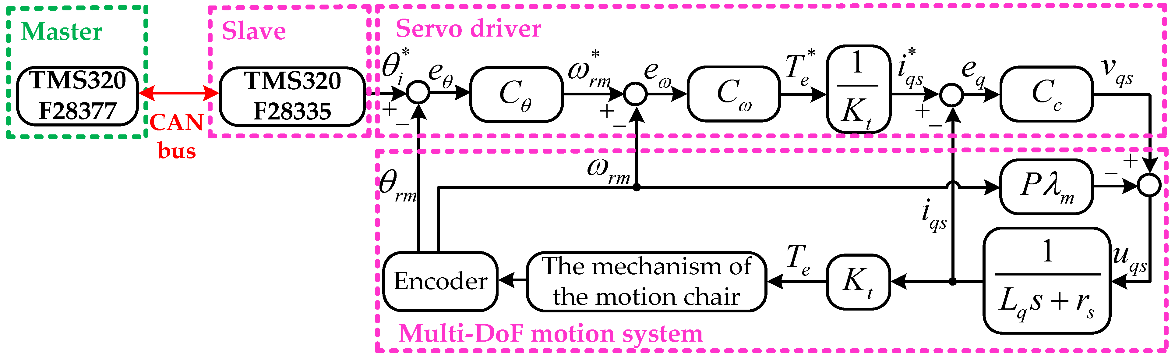
In this paper, the implementation of the three-axis motion system was based on the PID controller because of its simplicity and wide use in industrial applications. In addition, by suitably adjusting the gains $K_P$, $K_I$, and $K_D$, the controller can achieve the required performance of a closed-loop control system. A detailed description follows.

From the $d-q$ axis synchronous coordinate frame, the voltage equation is [31]:

$$v_{ds}=r_s{i}_{ds}+L_d\frac{d}{dt}{i}_{ds}-{\omega }_{re}{L}_q{i}_{qs}$$

(6)

$$v_{qs}=r_s{i}_{qs}+L_q\frac{d}{dt}{i}_{qs}+{\omega }_{re}{L}_d{i}_{ds}+{\omega }_{re}{\lambda }_m$$

(7)

where $v_{ds}$ and $v_{qs}$ are the $d$ axis and $q$ axis voltages, respectively, and $i_{ds}$ and $i_{qs}$ are the $d$ axis and $q$ axis currents, while $r_s$ is the resistance of motor, $L_d$ and $L_q$ are the inductances, ${\lambda }_m$ is the flux linkage, and ${\omega }_{re}$ is the electrical speed of motor. $i_{ds}$ = 0 is achievable with a field-oriented control. Then, Equations (6) and (7) can be rewritten as:

$$v_{ds}=-\left({\omega }_{re}{L}_q{i}_{qs}\right)$$

(8)

$$v_{qs}=r_s{i}_{qs}+L_q\frac{d}{dt}{i}_{qs}+{\omega }_{re}{\lambda }_m=u_q+{\omega }_{re}{\lambda }_m$$

(9)

The electromagnetic torque is expressed as follows:

$$T_e=\left(\frac{3}{2}\frac{P}{2}{\lambda }_m\right)\cdot i_{qs}=K_t\cdot i_{qs}$$

(10)

where $P$ is the number of poles of the motor and $K_t$ represents the torque constant. The dynamic mechanical equations of the rotor angle and rotor speed are expressed as:

$$\frac{d}{dt}{\theta }_{rm}={\omega }_{rm}$$

(11)

$$\frac{d}{dt}{\omega }_{rm}=\frac{1}{J_m}\left(T_e-T_L-B_m{\omega }_{rm}\right)$$

(12)

where $T_L$ is the external load, $B_m$ is the viscous coefficient of the motor, and $J_m$ is the moment of inertia of the motor. The electrical rotor speed and rotor angle are, respectively, expressed as follows:

$${\omega }_{re}=\frac{P}{2}{\omega }_{rm}$$

(13)

$${\theta }_{re}=\frac{P}{2}{\theta }_{rm}$$

(14)

The PID control law is

$$u=K_{P}e\left(t\right)+K_I{\displaystyle \int e\left(t\right)dt}+K_D\frac{d}{dt}e\left(t\right)$$

(15)

where $K_P$, $K_I$, and $K_D$ are the proportional coefficient, integral coefficient, and differential coefficient, respectively. The closed-loop control system is designed and applied independently to each actuator in the three degrees of freedom. In Figure 4, the control blocks $C_{\theta }$, $C_{\omega }$, and $C_c$ represent the PID controller for the position loop, speed loop, and current loop functions, respectively. The superscript “*” represents the reference command.

2.3. Encoder Error Compensation Embedded Executive

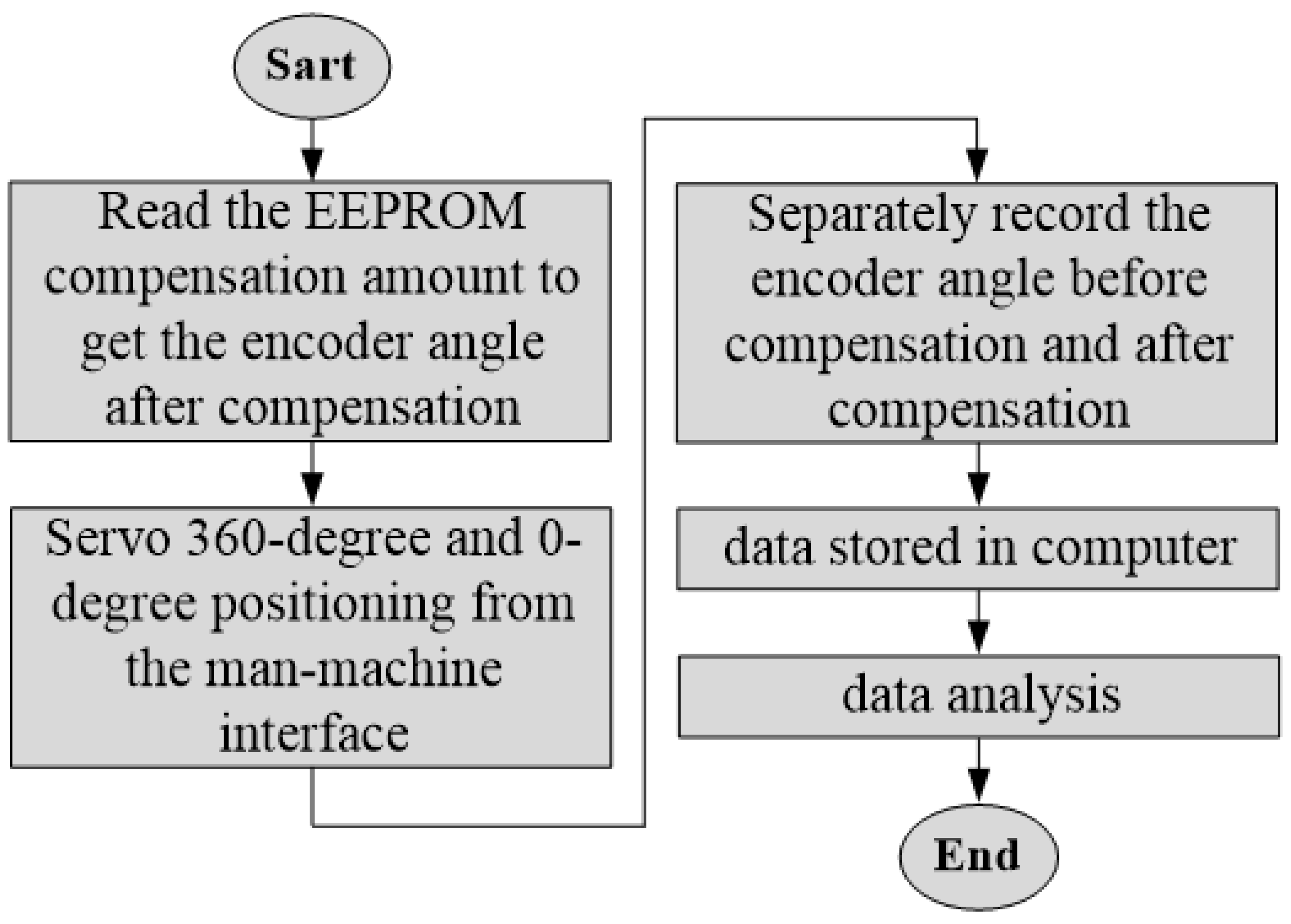
This paper uses a high-accuracy encoder as the basis for the proposed accuracy measurement. Figure 5 shows the flow chart of the measurement accuracy. At the initial stage of the program, it tries to read and write EEPROM. If the comparison model is correct, it means that the EEPROM has been burned and will write the compensation value for EEPROM. If the comparison is wrong, only the angle generated by the encoder is generated, and then the angle generated by the encoder is combined with the compensation value. Then, the engineer can operate the user interface to execute the motor forward and reverse one circle so that the DSP can record the angle information before and after compensation and calculate the error. After completion, the angle of the two encoders and the error value between the two is calculated and stored in the computer as a reference for the subsequent execution of the error compensation program.

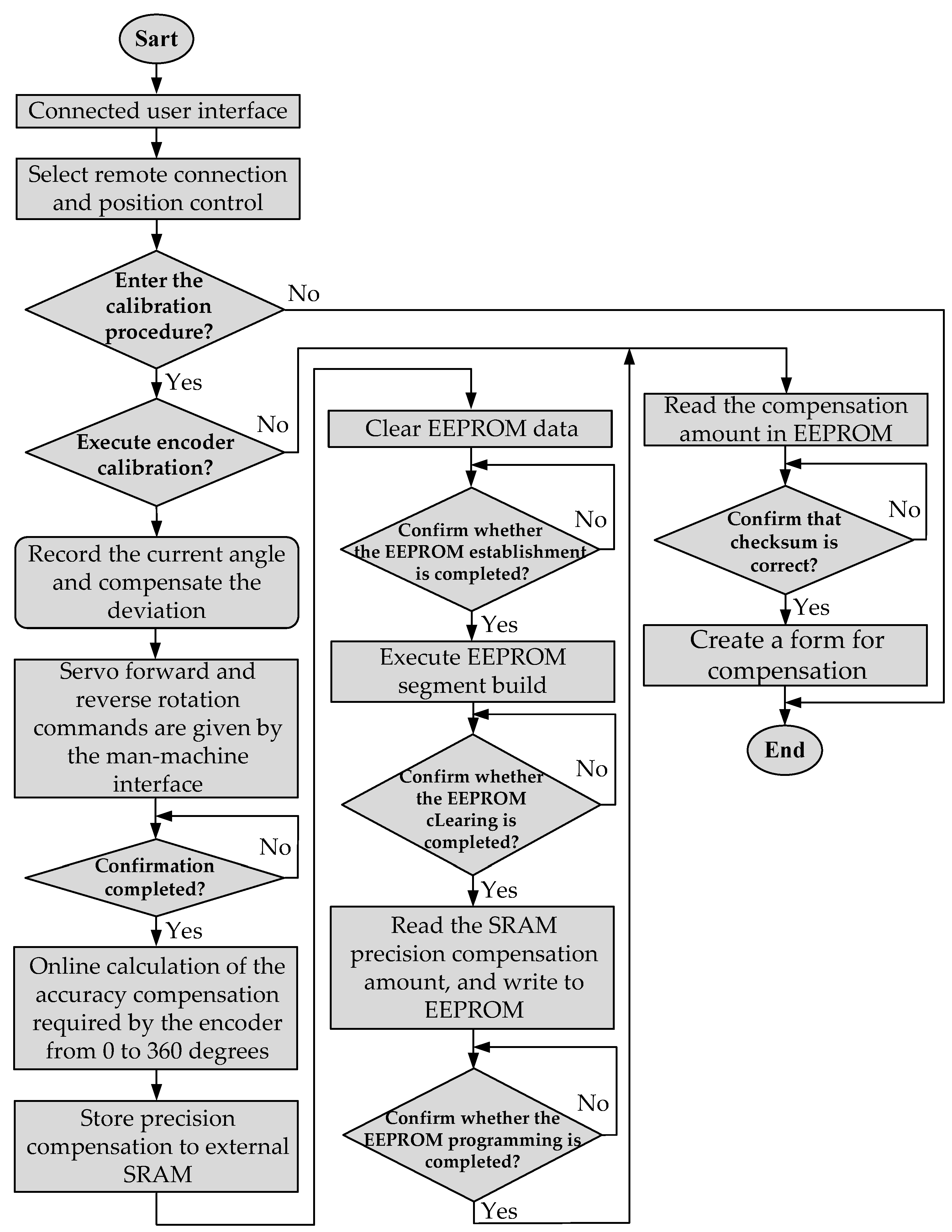
The accuracy of the general servo encoder is 50 arc seconds, and the high-accuracy encoder is selected as the reference standard for subsequent calibration. In this paper, the 5 arc-second relative photoelectric encoder is selected, and the error compensation flowchart is proposed as shown in Figure 6. The EEPROM is used to move and program the calibration data, and the external SRAM on the hardware is used as a buffer for data storage. During the process, a huge amount of data are stored here, and two encoders are stored in sequence. The forward rotation angle, reverse rotation angle, and processed compensation amount are stored in the buffer. After the buffer stores the three kinds of data, the EEPROM is programmed. After the programming is successful, the EEPROM can still be reused after power has been turned off and on.

Since this paper uses user interface software to issue operating instructions, it is necessary to implement the connection of the user interface before starting so that the RS422 interface channel can transmit and receive commands from the control end or server end in real time through messages, making operation possible. The user can obtain the current status of the servo in real time, and after the connection is confirmed, the user interface also sends messages to the server.

The motor displacement, angle obtained by the general encoder and high-accuracy encoder, and number of errors for each of the two are recorded by the test computer.

Because the accuracy of the general servo encoder is relatively low, the actual angle is generated internally every time it is used, but for the convenience of the operator, when the encoder is adjusted, the software compensates for the angle deviation to match general servo encoders in order to perform alignment with relative-type high-accuracy encoders.

Then, the user interface issues a position control command to the server and confirms again whether to start the adjustment procedure. If yes, the operator issues a position command for the motor to rotate 360 degrees forward through the user interface. At this time, the motor is positioned at 360 degrees, and the angles of the two encoders are recorded at the same time. After the positioning is completed, it is recorded through the user interface, and the motor is commanded to turn to the zero position; when the adjustment program is selected, it means that the compensation data inside the EEPROM will be read after the program starts. If it is confirmed that the check code is correct, the compensation amount will be used to match the general encoder angle.

The calculation of the compensation amount uses the two kinds of encoder angles recorded during the motor positioning process and calculates the compensation amount for different angles via the interpolation method [32]. After the low-accuracy encoder data are established, there are three internal addresses; the data are stored in the external SRAM, the EEPROM is internally cleared, and the EEPROM storage section is created. When all sections are established, the software automatically communicates the compensation value of the external SRAM to the EEPROM via RS485.

3. Kinematics Relations

The real three-degree-of-freedom platform is shown in Figure 1. It can be seen from the figure that the rotary cabin and the turntable of the platform provide two degrees of freedom for the pitch axis and the yaw axis, respectively, and the other degree of freedom is the linear motion effect generated by the surge axis. To obtain the coordinate transformation relation as

$$\left[\begin{array}{c}{x}_f\\ y_f\\ z_f\end{array}\right]=\left[\begin{array}{ccc}\cos \alpha & 0& \sin \alpha \\ 0& 1& 0\\ -\sin \alpha & 0& \cos \alpha \end{array}\right]\left[\begin{array}{c}{x}_1\\ y_1\\ z_1\end{array}\right]$$

(16)

$$\left[\begin{array}{c}{x}_1\\ y_1\\ z_1\end{array}\right]=\left[\begin{array}{ccc}\cos \beta & -\sin \beta & 0\\ \sin \beta & \cos \beta & 0\\ 0& 0& 1\end{array}\right]\left[\begin{array}{c}{x}_B\\ y_B\\ z_B\end{array}\right]$$

(17)

where $\alpha$ and $\beta$ are Euler angles rotated in the order of pitch and yaw, respectively.

The inertial coordinate vector can be clearly expressed as the body coordinate vector by the transformation relationship of Equations (16) and (17), written as

$$p^I=R_{\mathsf{\Theta }}{p}^B$$

(18)

where $R_{\mathsf{\Theta }}$ is the rotation matrix, depending on the Euler angle $\mathsf{\Theta }$, from the body frame to the inertial frame, and convention expressed as

$$R_{\mathsf{\Theta }}=R_y{R}_z$$

(19)

where $R_y$ and $R_z$ are represented as rotation matrices for the pitch and yaw axes.

Substituting Equation (19) into Equations (16) and (17), one can obtain

$$\begin{array}{l}{R}_{\mathsf{\Theta }}=\left[\begin{array}{ccc}\cos \alpha & 0& \sin \alpha \\ 0& 1& 0\\ -\sin \alpha & 0& \cos \alpha \end{array}\right]\left[\begin{array}{ccc}\cos \beta & -\sin \beta & 0\\ \sin \beta & \cos \beta & 0\\ 0& 0& 1\end{array}\right]\\ =\left[\begin{array}{ccc}\left(\cos \beta \cos \alpha \right)& -\left(\cos \alpha \sin \beta \right)& \sin \alpha \\ \sin \beta & \cos \beta & 0\\ -\left(\cos \beta \sin \alpha \right)& \sin \beta \sin \alpha & \cos \alpha \end{array}\right]\end{array}$$

(20)

The transformation matrix of the inertial coordinates $T_{\mathsf{\Theta }}$ is

$$\begin{array}{l}{T}_{\mathsf{\Theta }}=\left[\begin{array}{cccc}\left(\cos \beta \cos \alpha \right)& -\left(\cos \alpha \sin \beta \right)& \left(\sin \alpha \right)& x\\ \left(\sin \beta \right)& \left(\cos \psi \right)& 0& y\\ -\left(\cos \beta \sin \alpha \right)& \left(\sin \beta \sin \alpha \right)& \left(\cos \alpha \right)& z\\ 0& 0& 0& 1\end{array}\right]\\ =\left[\begin{array}{cccc}{x}_x& y_x& z_x& p_x\\ x_y& y_y& z_y& p_y\\ x_z& y_z& z_z& p_z\\ 0& 0& 0& 1\end{array}\right]\end{array}$$

(21)

The angular velocity of the body frame rotation is expressed as

$${\stackrel{\rightharpoonup }{\omega }}^B={\left[\begin{array}{ccc}p& q& r\end{array}\right]}^T$$

(22)

The rotational angular velocity of the axis coordinates is written as

$$\dot{\mathsf{\Phi }}={\left[\begin{array}{cc}\dot{\alpha }& \dot{\beta }\end{array}\right]}^T$$

(23)

After rearranging Equations (22) and (23), we can obtain

$$p\cdot \left({\stackrel{\rightharpoonup }{x}}_B\right)+q\cdot \left({\stackrel{\rightharpoonup }{y}}_B\right)+r\cdot \left({\stackrel{\rightharpoonup }{z}}_B\right)=\dot{\alpha }\cdot \left({\stackrel{\rightharpoonup }{y}}_1\right)+\dot{\beta }\cdot \left({\stackrel{\rightharpoonup }{z}}_B\right)$$

(24)

Substitute Equation (17) into Equation (24) as follows

$$p\cdot \left({\stackrel{\rightharpoonup }{x}}_B\right)+q\cdot \left({\stackrel{\rightharpoonup }{y}}_B\right)+r\cdot \left({\stackrel{\rightharpoonup }{z}}_B\right)=\left(\dot{\alpha }\sin \beta \right){\stackrel{\rightharpoonup }{x}}_B+\left(\dot{\alpha }\cos \beta \right){\stackrel{\rightharpoonup }{y}}_B+\left(\dot{\beta }\right){\stackrel{\rightharpoonup }{z}}_B$$

(25)

Then, the rotation angular velocity of the body coordinates of the simulator is converted via the rotation angular velocity of the axis coordinates, and it can be obtained

$$\left[\begin{array}{c}p\\ q\\ r\end{array}\right]=\left[\begin{array}{cc}\left(\sin \beta \right)& 0\\ \left(\cos \beta \right)& 0\\ 0& 1\end{array}\right]\left[\begin{array}{c}\dot{\alpha }\\ \dot{\beta }\end{array}\right]$$

(26)

Next, position $(p_x,p_y,p_z)$, attitude $\stackrel{\rightharpoonup }{x}$ in the x direction, attitude $\stackrel{\rightharpoonup }{y}$ in the y direction, and attitude $\stackrel{\rightharpoonup }{z}$ in the z direction are found via computing the axis coordinates $(x,\alpha ,\beta )$ of the platform. Thus, Equation (20) can be obtained

$$R_z=R_y^{-1}{R}_{\mathsf{\Theta }}=\left[\begin{array}{ccc}\left(\cos \beta \right)& -\left(\sin \beta \right)& 0\\ \left(\sin \beta \right)& \left(\cos \beta \right)& 0\\ 0& 0& 1\end{array}\right]$$

(27)

Formula (21) contains attitude $\stackrel{\rightharpoonup }{x}$ in the x direction, attitude $\stackrel{\rightharpoonup }{y}$ in the y direction, and attitude $\stackrel{\rightharpoonup }{z}$ in the z direction. From this, we can obtain

$$\begin{array}{l}\left[\begin{array}{ccc}{x}_x\left(\cos \alpha \right)-x_z\left(\sin \alpha \right)& y_x{x}_x\left(\cos \alpha \right)-y_z\left(\sin \alpha \right)& z_x\left(\cos \alpha \right)-z_z\left(\sin \alpha \right)\\ x_y& y_y& z_y\\ x_x\left(\sin \alpha \right)+n_z\left(\cos \alpha \right)& y_x\left(\sin \alpha \right)+y_z\left(\cos \alpha \right)& z_x\left(\sin \theta \right)+z_z\left(\cos \alpha \right)\end{array}\right]\\ =\left[\begin{array}{ccc}\left(\cos \beta \right)& -\left(\sin \beta \right)& 0\\ \left(\sin \beta \right)& \left(\cos \beta \right)& 0\\ 0& 0& 1\end{array}\right]\end{array}$$

(28)

Next, Equation (28) can be expressed as

$$z_x\left(\cos \alpha \right)-z_z\left(\sin \alpha \right)=0$$

(29)

$$z_x\left(\sin \alpha \right)+z_z\left(\cos \alpha \right)=1$$

(30)

Then, it is not difficult to obtain the rotation angle of the pitch axis from Equations (29) and (30), which can be expressed as

$$\alpha {=\tan }^{-1}\left(\frac{z_x}{z_z}\right)$$

(31)

The relationship of Equation (28) can be expressed as

$$\left(\sin \beta \right)=\left(-y_x{x}_x\left(\cos \alpha \right)+y_z\left(\sin \alpha \right)\right)$$

(32)

$$\left(\cos \beta \right)=\left(x_x\left(\cos \alpha \right)-x_z\left(\sin \alpha \right)\right)$$

(33)

The yaw axis angle from Equations (32) and (33) can be obtained

$$\tan \beta =\left(\frac{\sin \beta }{\cos \beta }\right)=\left[\frac{-y_x{x}_x\left(\cos \alpha \right)+y_z\left(\sin \alpha \right)}{x_x\left(\cos \alpha \right)-x_z\left(\sin \alpha \right)}\right]$$

(34)

The above formula taking the arc tangent function is

$$\beta ={\tan }^{-1}\left(\frac{-y_x{x}_x\left(\cos \alpha \right)+y_z\left(\sin \alpha \right)}{x_x\left(\cos \alpha \right)-x_z\left(\sin \alpha \right)}\right)$$

(35)

By using the Equations (31) and (35), the coordinates of the rotation axis of the three-axis platform are obtained. Equation (21) can express the surge axis coordinates as

$$x=p_x$$

(36)

4. Monitoring System

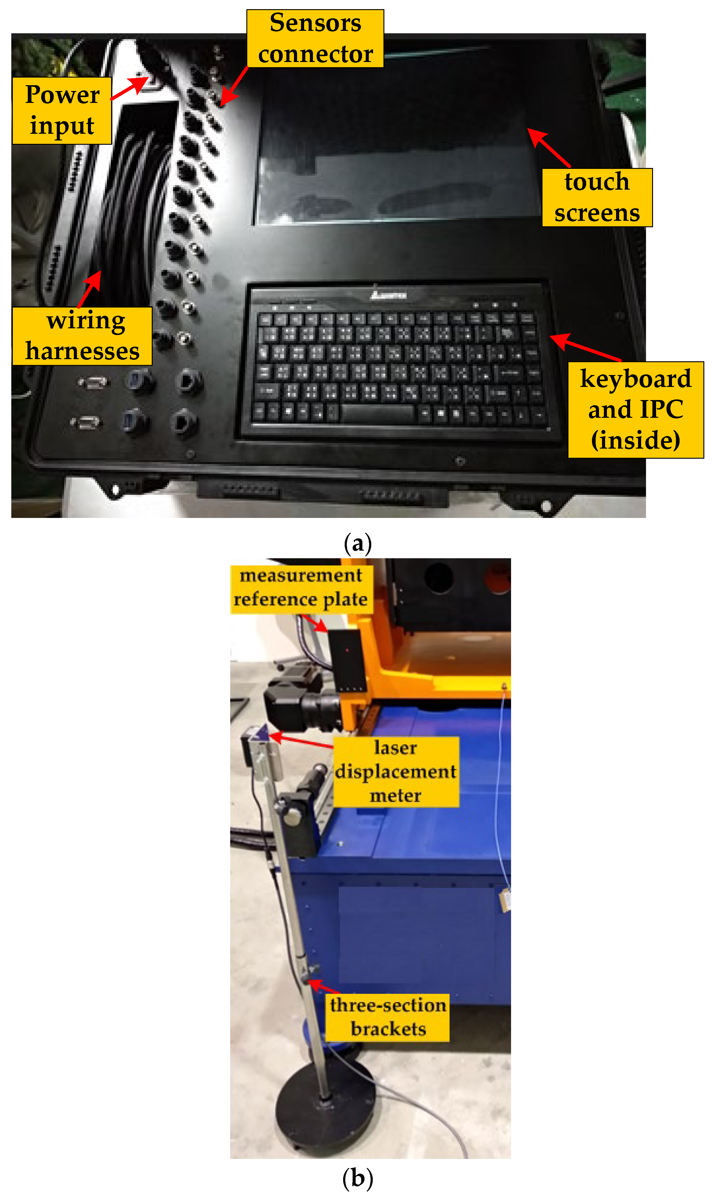
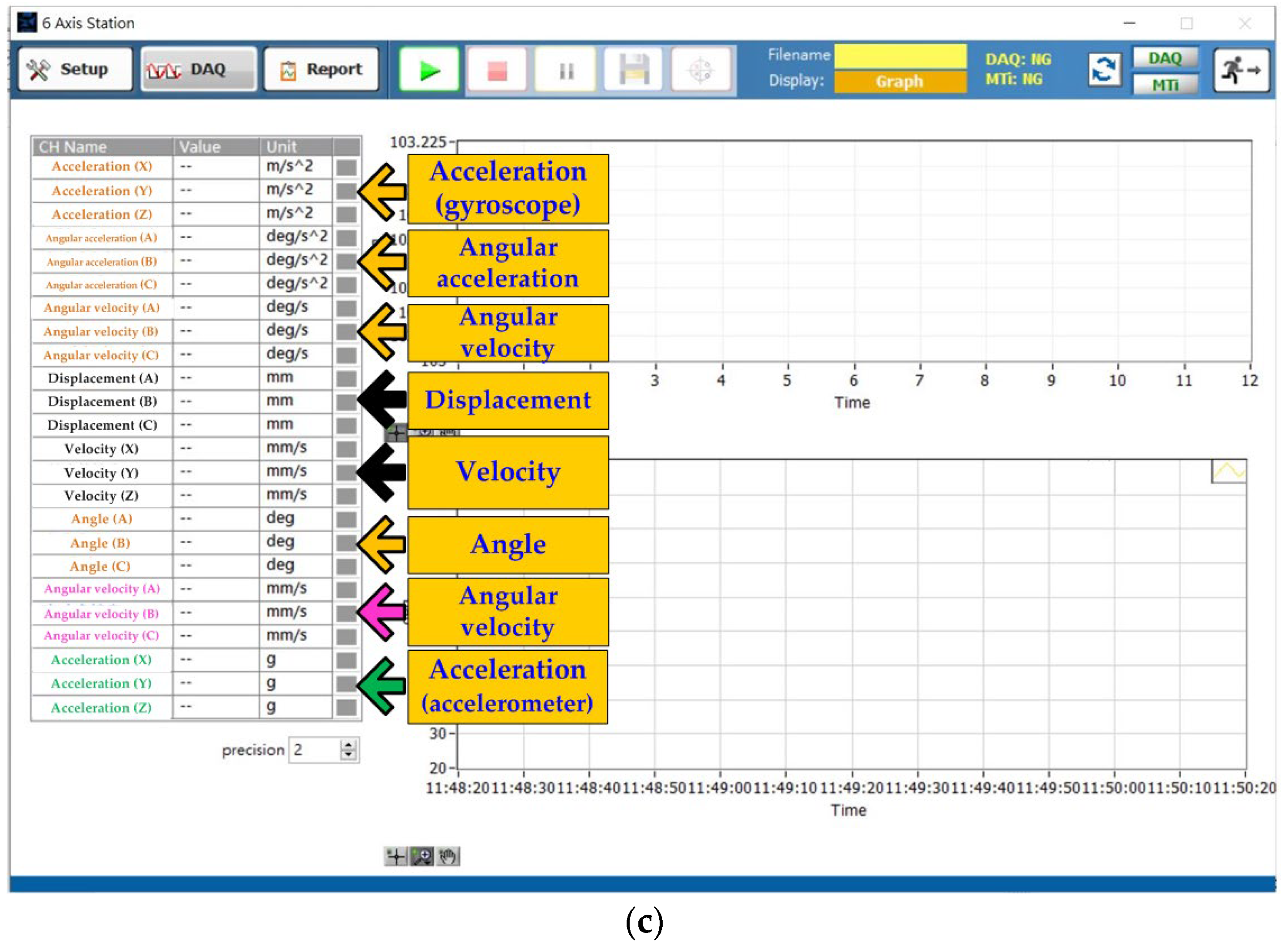
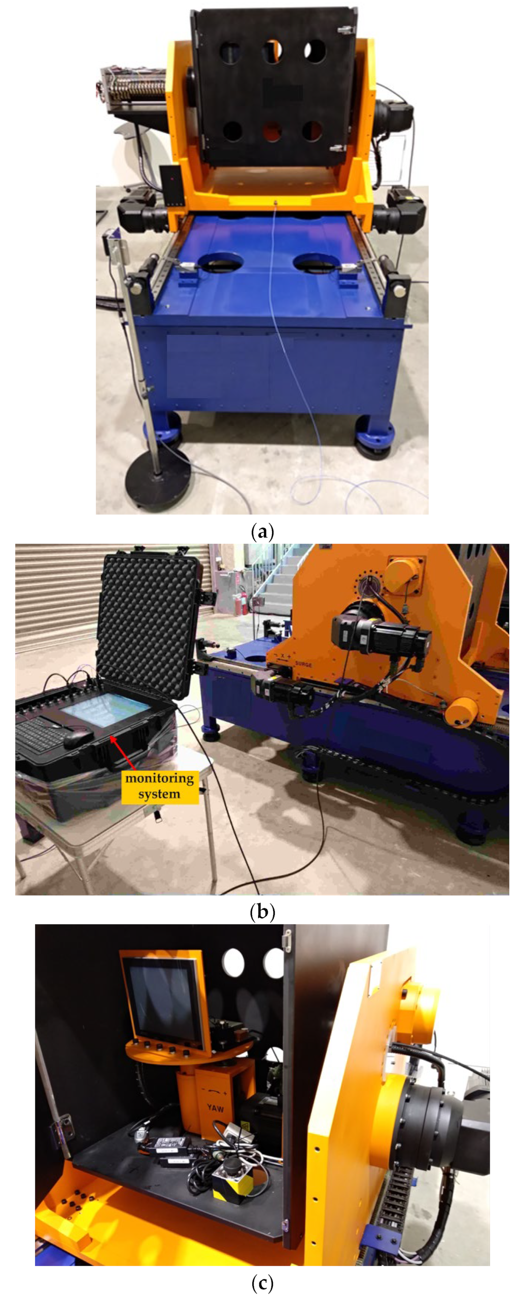
The monitoring system mainly tests the characteristics of the motion platform as shown in Figure 7a–c. An industrial computer is used to write the monitoring software of the LabVIEW environment. Figure 7a shows the appearance of the monitoring system. The waterproof box contains high-speed data collectors, industrial computers (IPCs), touchscreens, sensors, professional wiring harnesses, fixtures, etc. The measurement software can be written to measure and record various parameters of the three-axis motion platform at high speed. Figure 7b shows that the laser displacement meter reads the moving position signal by hitting the center of the reference plate with the red laser light emitted, so it includes a three-section bracket that can adjust the height of the laser displacement meter and a measurement reference plate with magnetic adhesion to the three-axis platform. The setup form of the measurement software includes measurement speed settings and archive paths. The settings related to the sensor are as follows: the laser displacement meter for measuring displacement uses the voltage input channel to receive the position signal (the software enables or disables this function and adjusts the channel name, scale, offset, and unit), and the attitude gyroscope adopts RS232 serial signal transmission and reception. Figure 7c shows the real-time curve drawn by the signal received by the sensor used. On the left side of the screen are different display channels. The tester can perform continuous and simultaneous measurement, display, and archiving by clicking on the channel to be measured.

5. Implementation

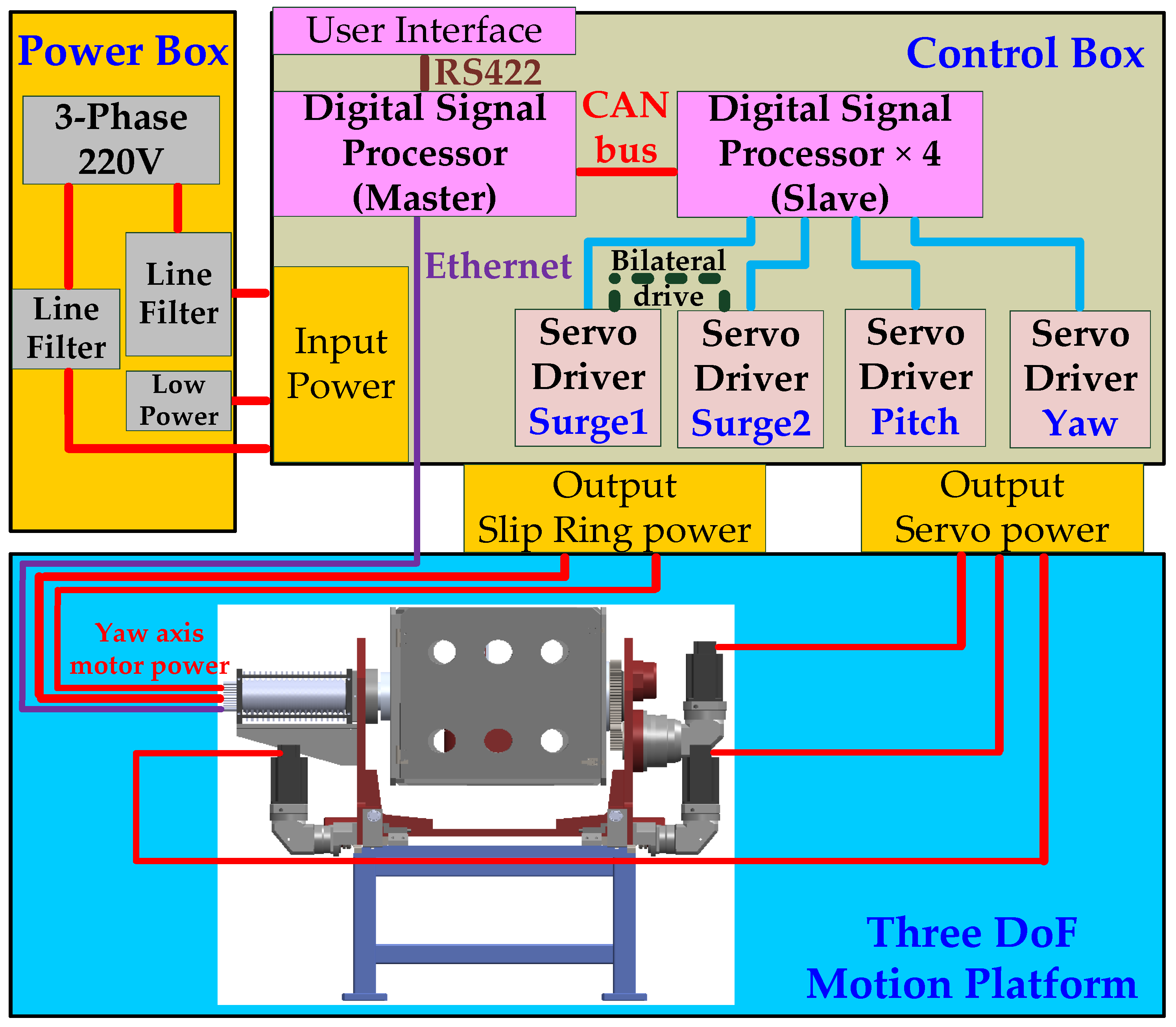
The block diagram of the three-axis motion platform is shown in Figure 8. Considering that the three-axis platform has a linear bilateral drive and a continuous rotation drive, in the continuous rotation, the power and signal are transmitted to the rotary cabin through the slip ring for the use of the turntable to generate the movement of the yaw axis. It can be seen from the observation in Figure 9 that it is mainly composed of the body mechanism, the power box, and the control box. The body mechanism is composed of a rotary cabin, a turntable, a slip ring, five reducers, five motors, a positioning low-accuracy encoder, two slide rails, two racks, four oil pressure buffers, and four micro switches. The power box adopts a 3-phase 4-wire 220 V, 200 A design as the power source of the platform, while the control box uses a digital signal processor (TMS320F28377D) as the master control terminal and 4 digital signal processors (TMS320F28335) as the core of the slave control and completes peripheral hardware and software design. The relevant instructions are as follows:

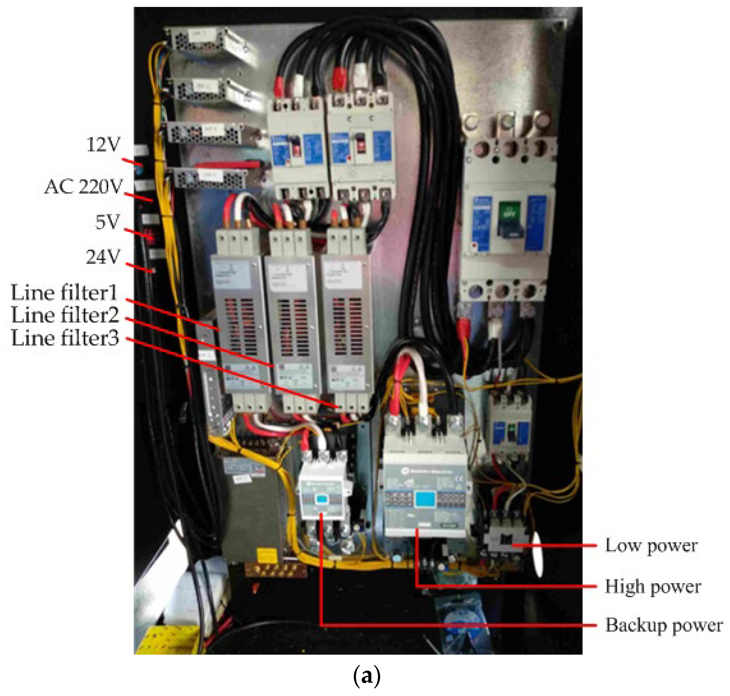
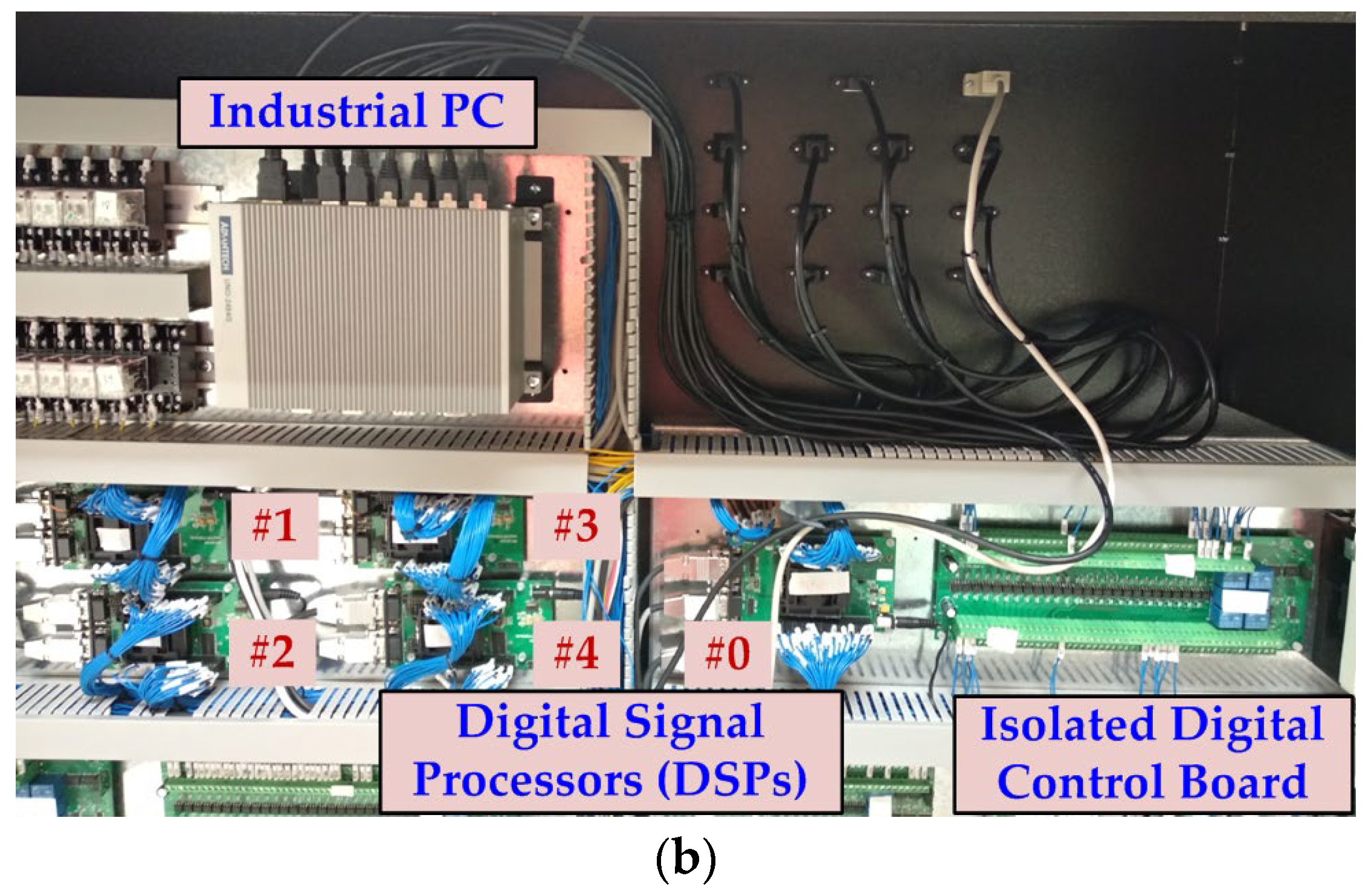
Inside the power box, the 220-volt power supply is divided into low power supply and high power supply, as shown in Figure 10a. The small battery converts 220 volts into 5 volts, 12 volts, and 24 volts through a power converter, and they are used as the internal circuit board of the control box, brake power supply, positioning encoder, and power relay, respectively. A transformer is then used to convert the supply into a 110-volt power supply for external sockets; the high power supply is mainly used for 4 sets of servo drives and motors, and the drives are placed on the back of the control box. The high power supply is used by three sets of servos for the surge axis of the linear stroke and the pitch axis and yaw axis of the roll type stroke. Therefore, it can be seen from Figure 10a that there will be 4 leakage circuit breakers, namely the main circuit breaker 200 A, 2 sets of servo circuit breakers 125 A, 3 sets of servo circuit breakers 50 A, and small circuit breakers 30 A. Then, 3 noise filters generate stable 3-phase 220 volts for the servo. Five digital signal processors are installed inside the control box. The first digital signal processor (#0, TMS320F28377D) uses a clock pulse of 200 MHz produced by Texas Instruments. It is responsible for the internal and external communication of the control box. The positioning, speed, and torque commands required by the six-axis servo are sent, and the six-axis servo status, working mode, and connection status are received. Externally, the RS422 interface mainly receives the operation commands sent by the user interface. The remaining four blocks use digital signal processors (#1–#4, TMS320F28335) produced by Texas Instruments with a clock pulse of 150 MHz to control the 3-degree-of-freedom servos and can issue control modes and control commands to the drives to be executed. The type of digital control board transmits to and receives the DI/DO signal from the digital signal processor, and the digital signal processor issues servo control commands to the driver, as shown in Figure 10b.

Table 1. Parameters of the motor.

	DOF	Surge1	Surge2	Pitch	Yaw
Item
Power dissipation (kW)		1.5	1.5	1.5	1.0
Rated Voltage (V)		220	220	220	220
Rated Current (A)		7.3	7.3	7.3	5.1
Rotor inertia (kg-cm2)		9.58	9.58	9.58	6.96
Rated speed		2000	2000	2000	2000
Maximum Speed (r/min)		2500	2500	2500	2500
Rated Torque (N.m)		7.16	7.16	7.16	4.77
Maximum Torque (N.m)		21.48	21.48	21.48	14.31
Reduction ratio of direct link reducer		1:14	1:14	1:50	1:20

shows the parameters of the motor.

Figure 11a shows the photograph of the three-axis motion platform and laser displacement meter. The operator opens the waterproof storage box and screws one end of the wire harness into the connector and the other end into sensor a, and the position of the measurement reference plate and the three-section bracket can be seen. Figure 11b shows the dynamic performance of the detection platform using the monitoring system. The inside of rotary cabin includes a reducer, a motor, and a set of test screens to detect the electrical signal of the slip ring, as shown in Figure 11c.

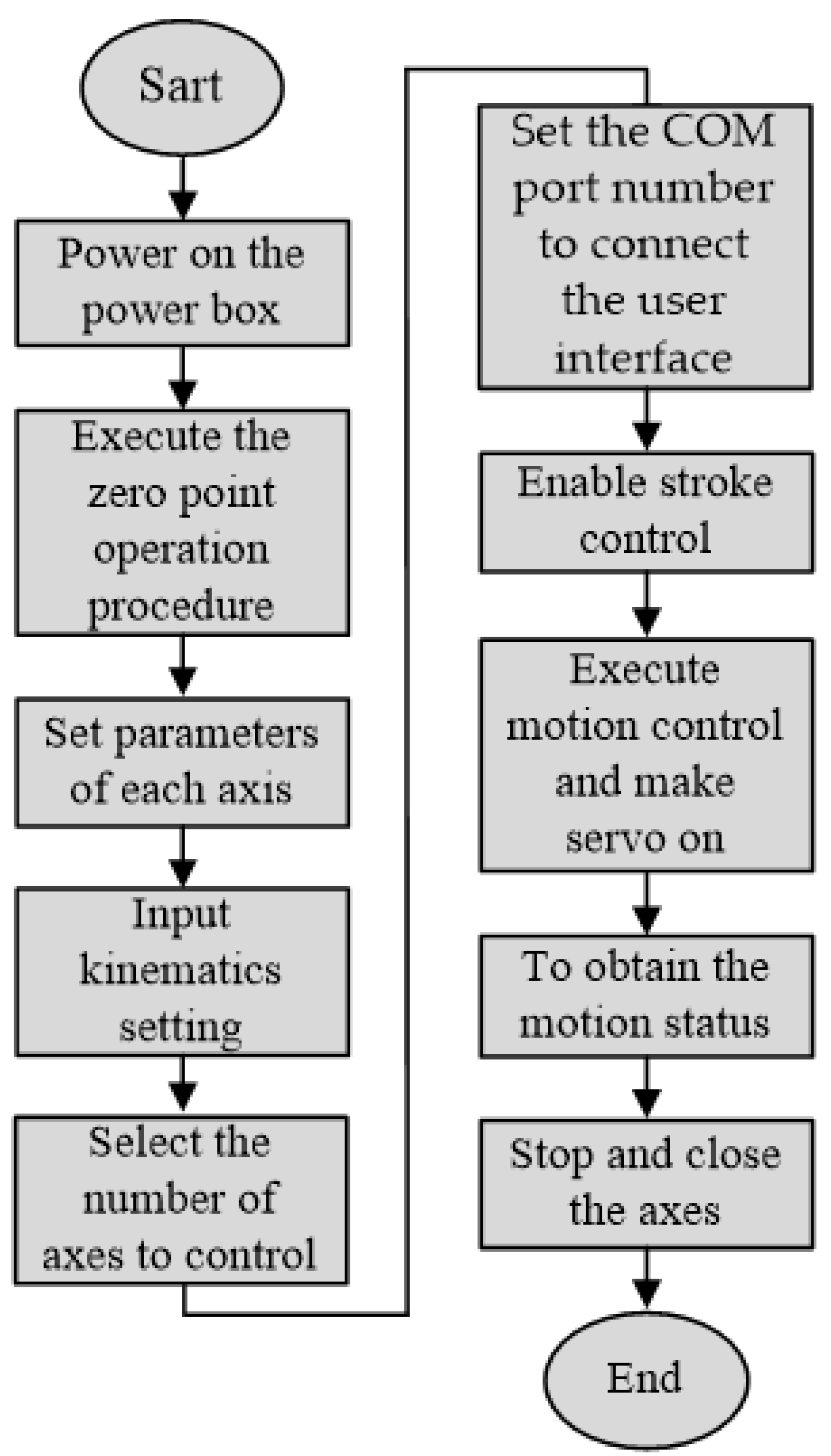
The control flow chart of the motion platform is shown in Figure 12. After the power box is powered on, the initial position of the servo motor of each axis will be read first. After inputting system parameters and performing kinematics, selecting the number of axes to drive, and connecting to the COM port of the user interface, the servo is enabled for stroke control, and the user interface inputs commands and monitors the running status of each axis.

6. Experimental Results

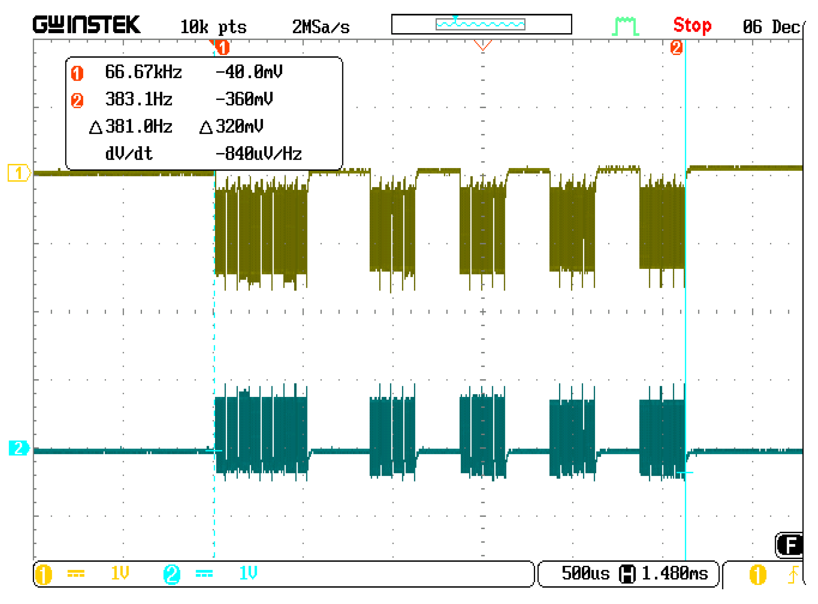
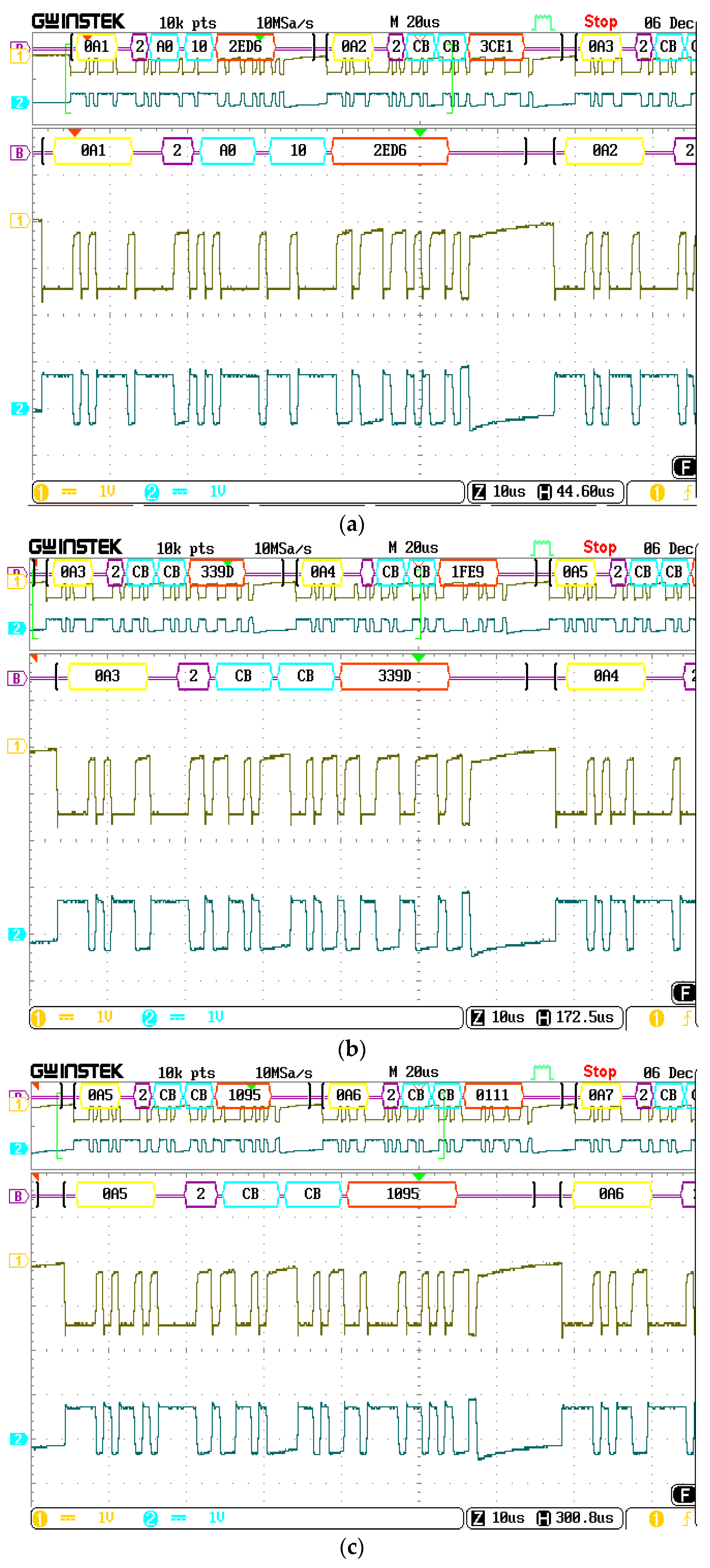
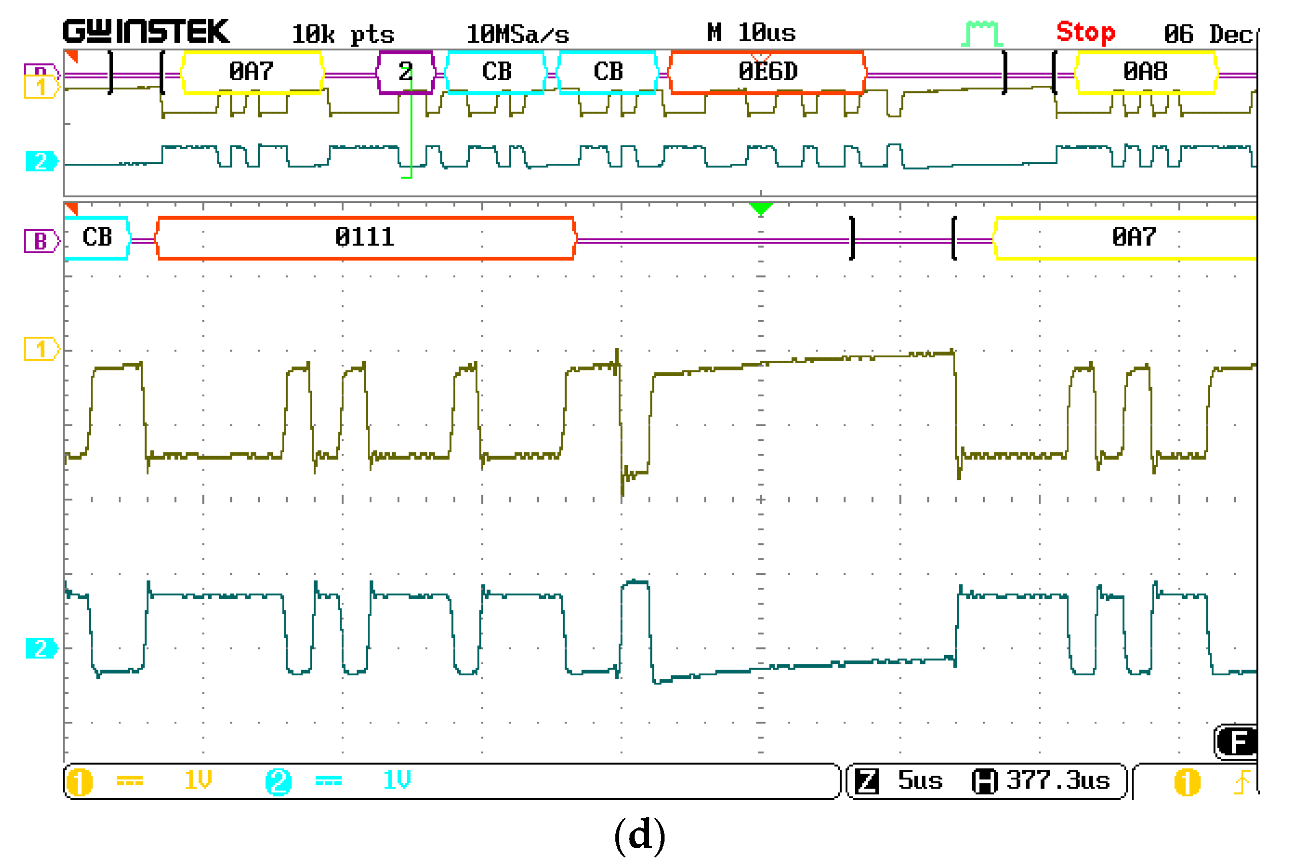
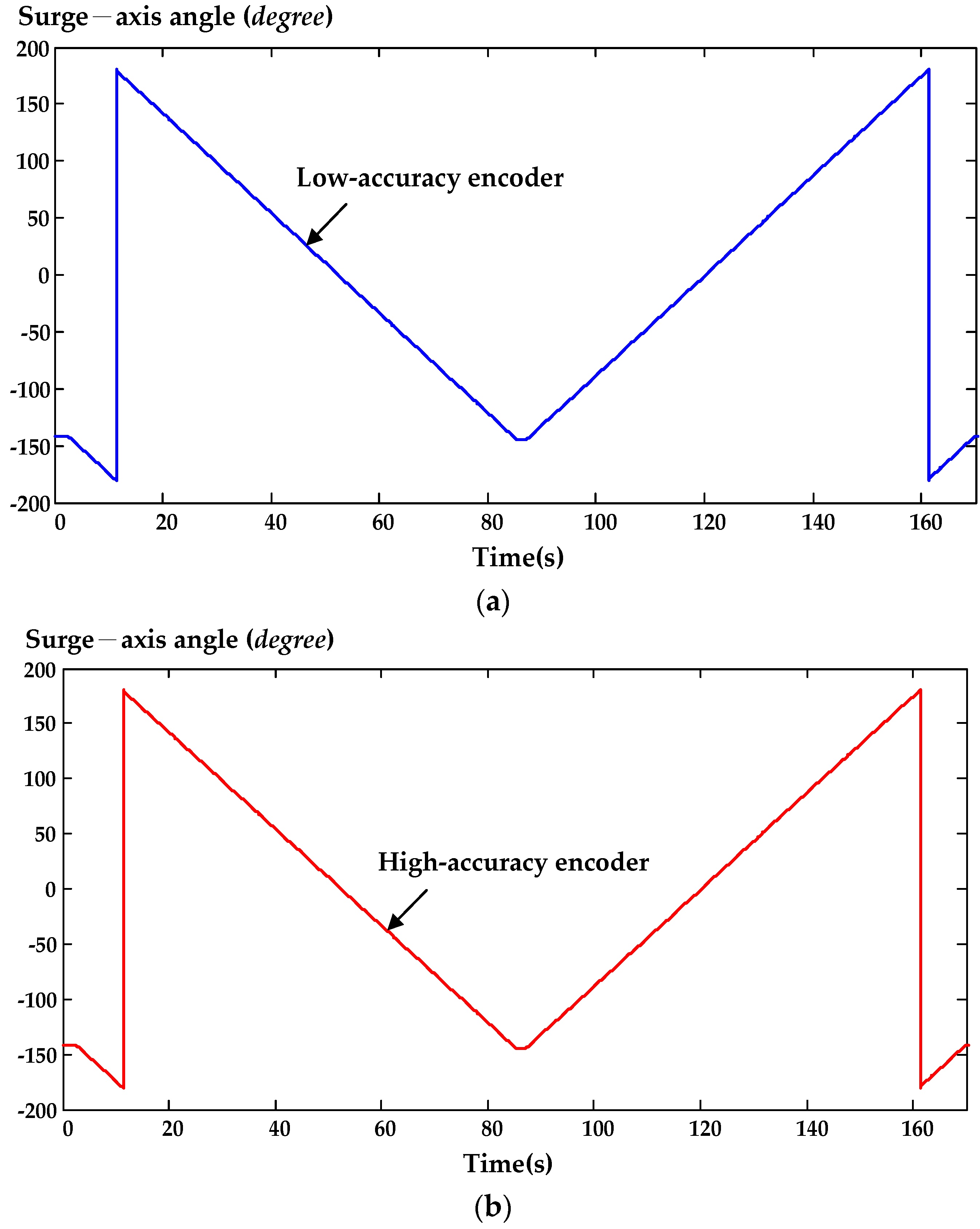
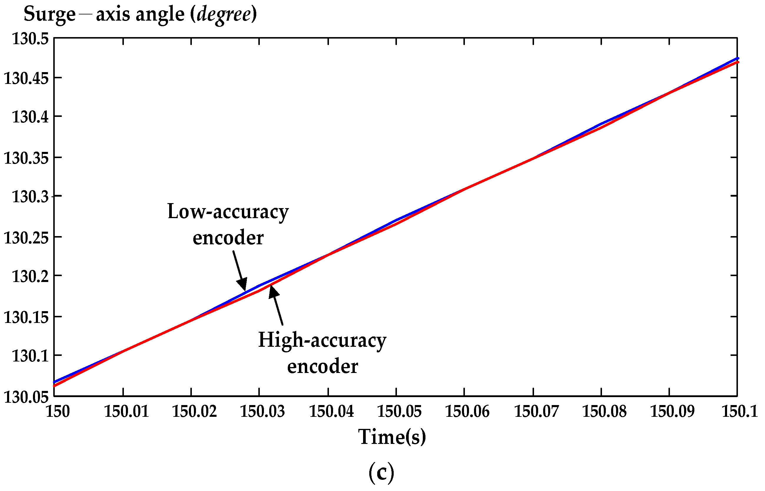
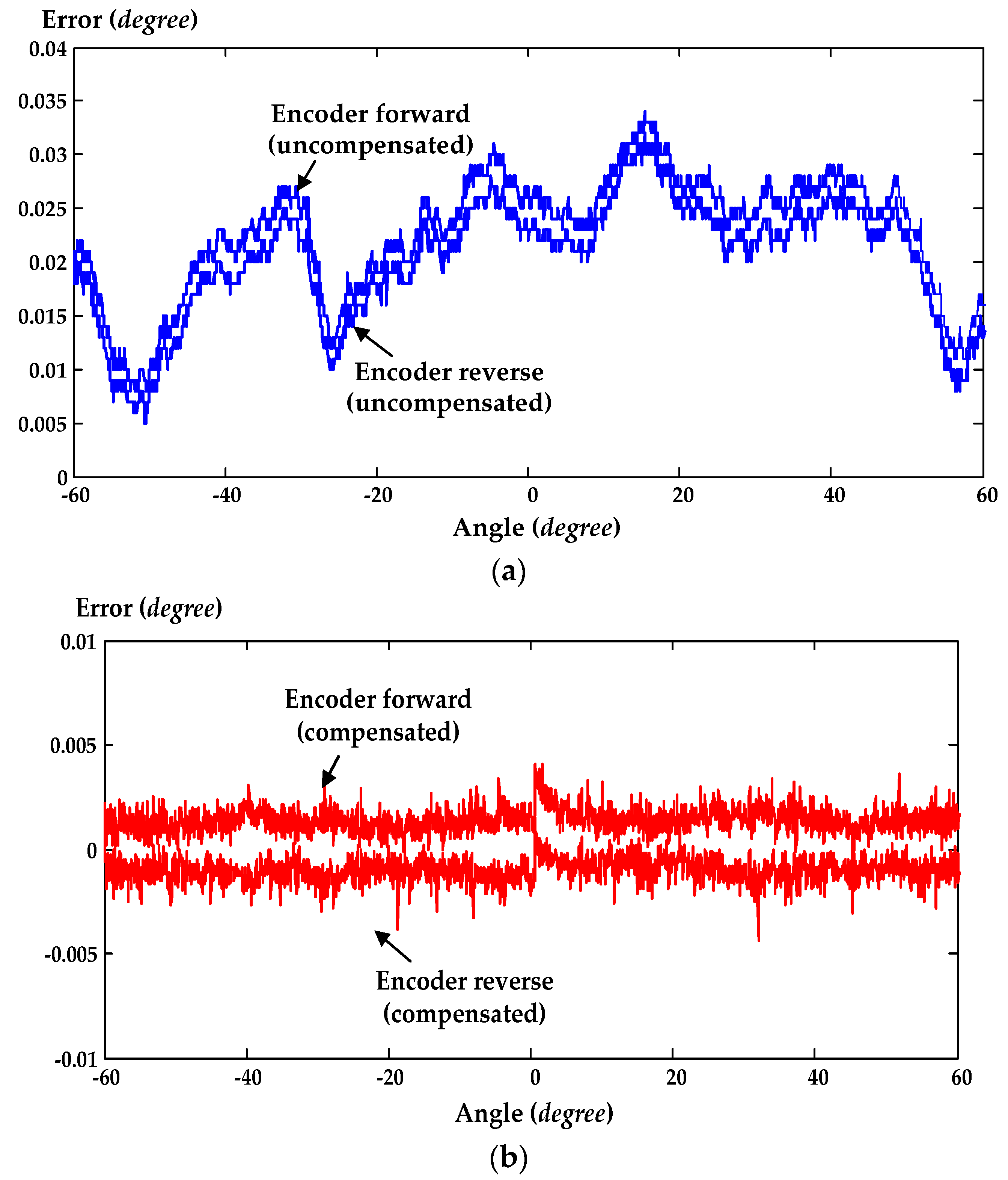
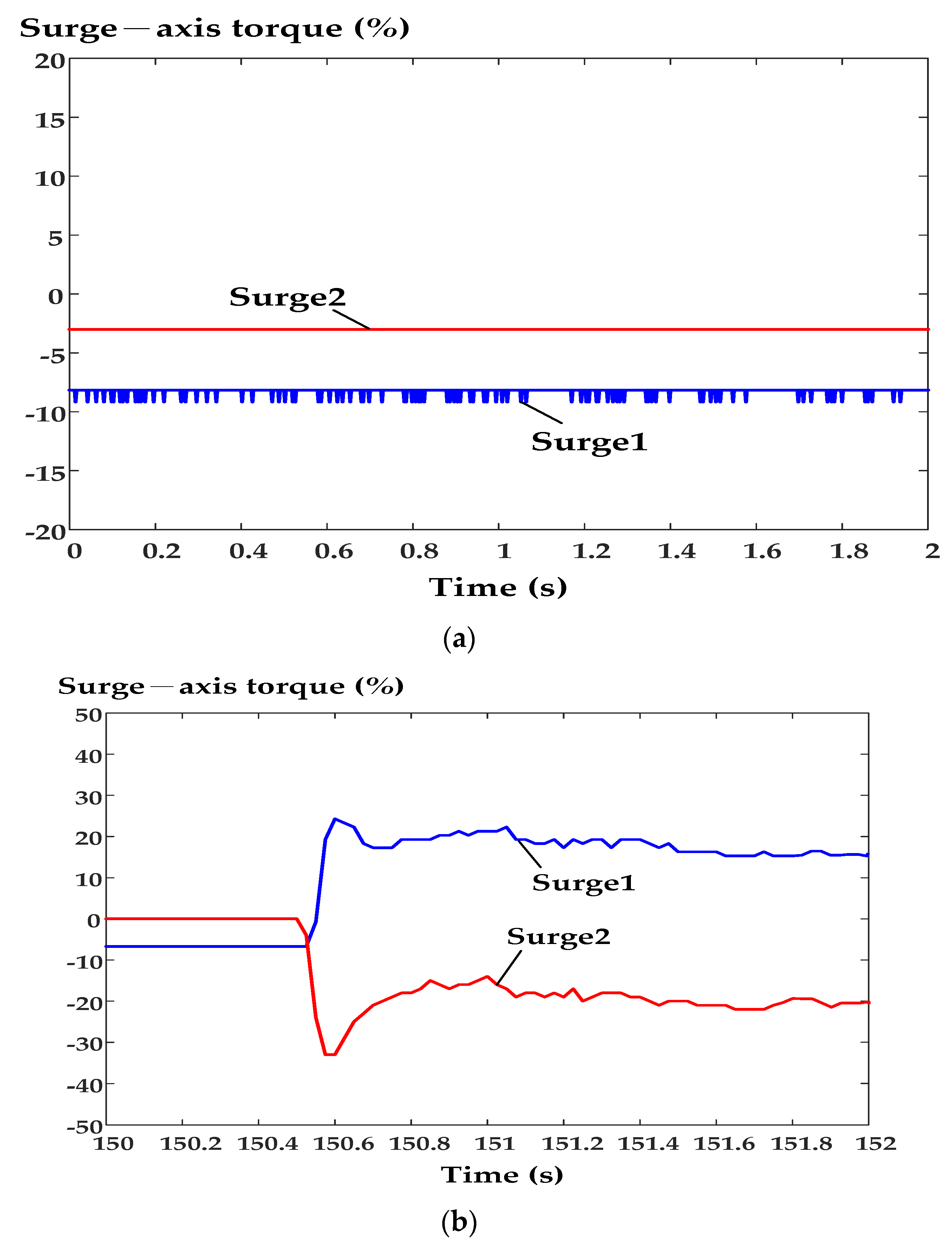
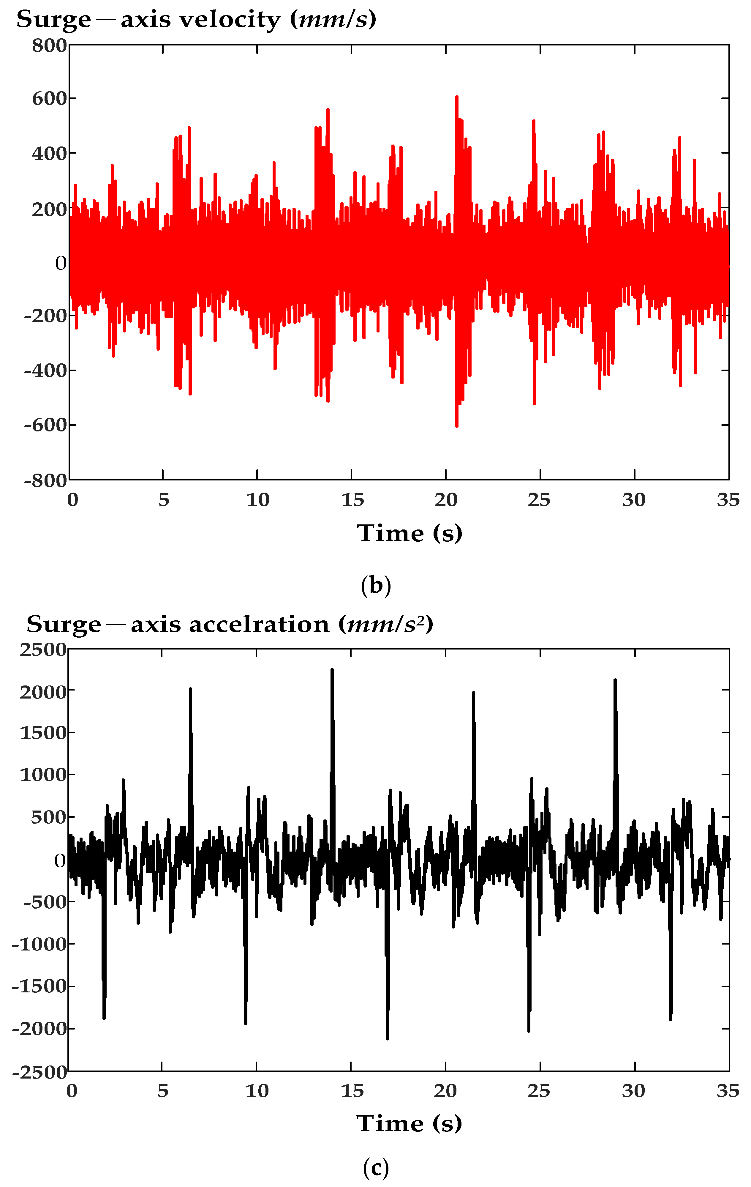
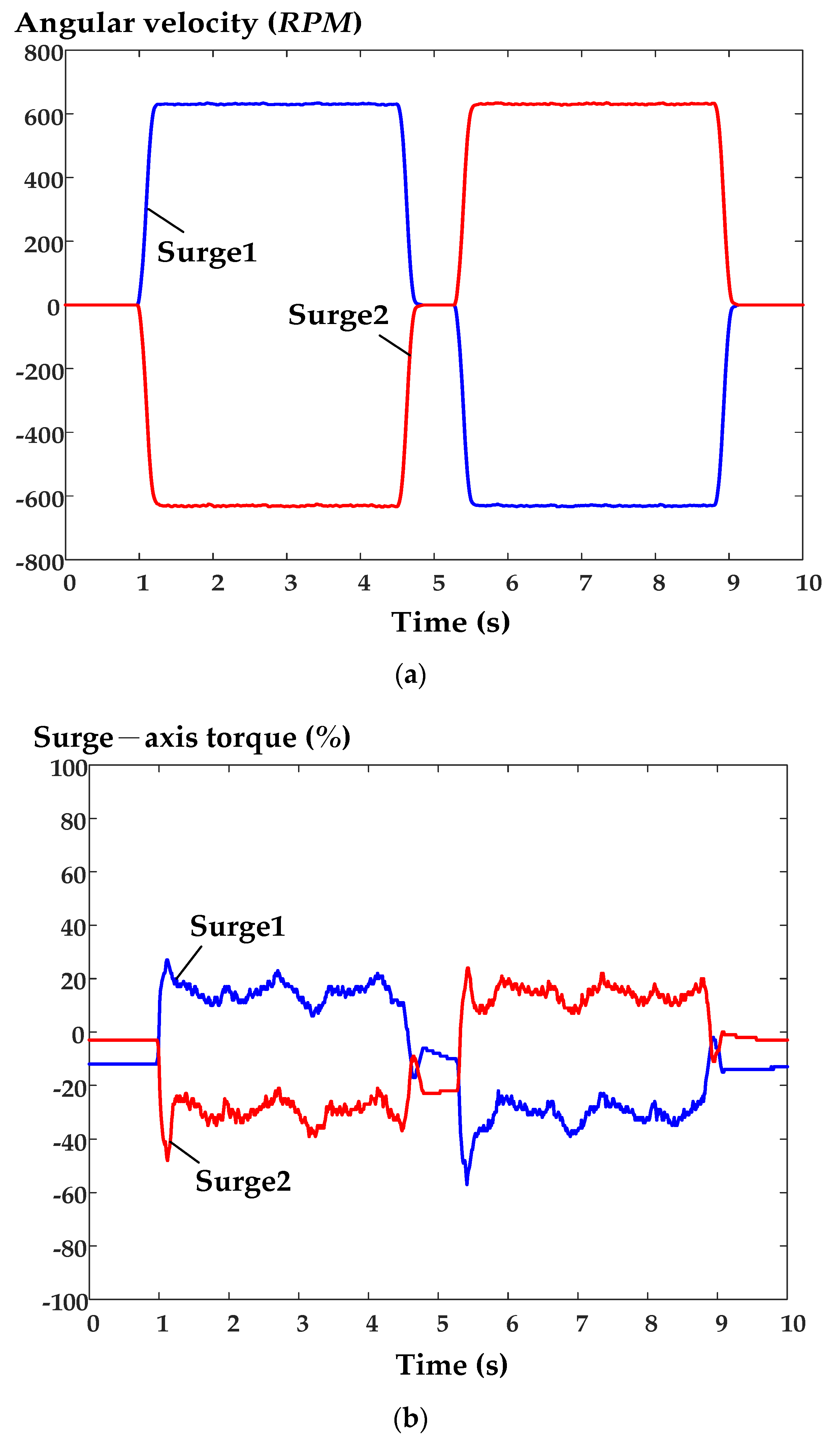
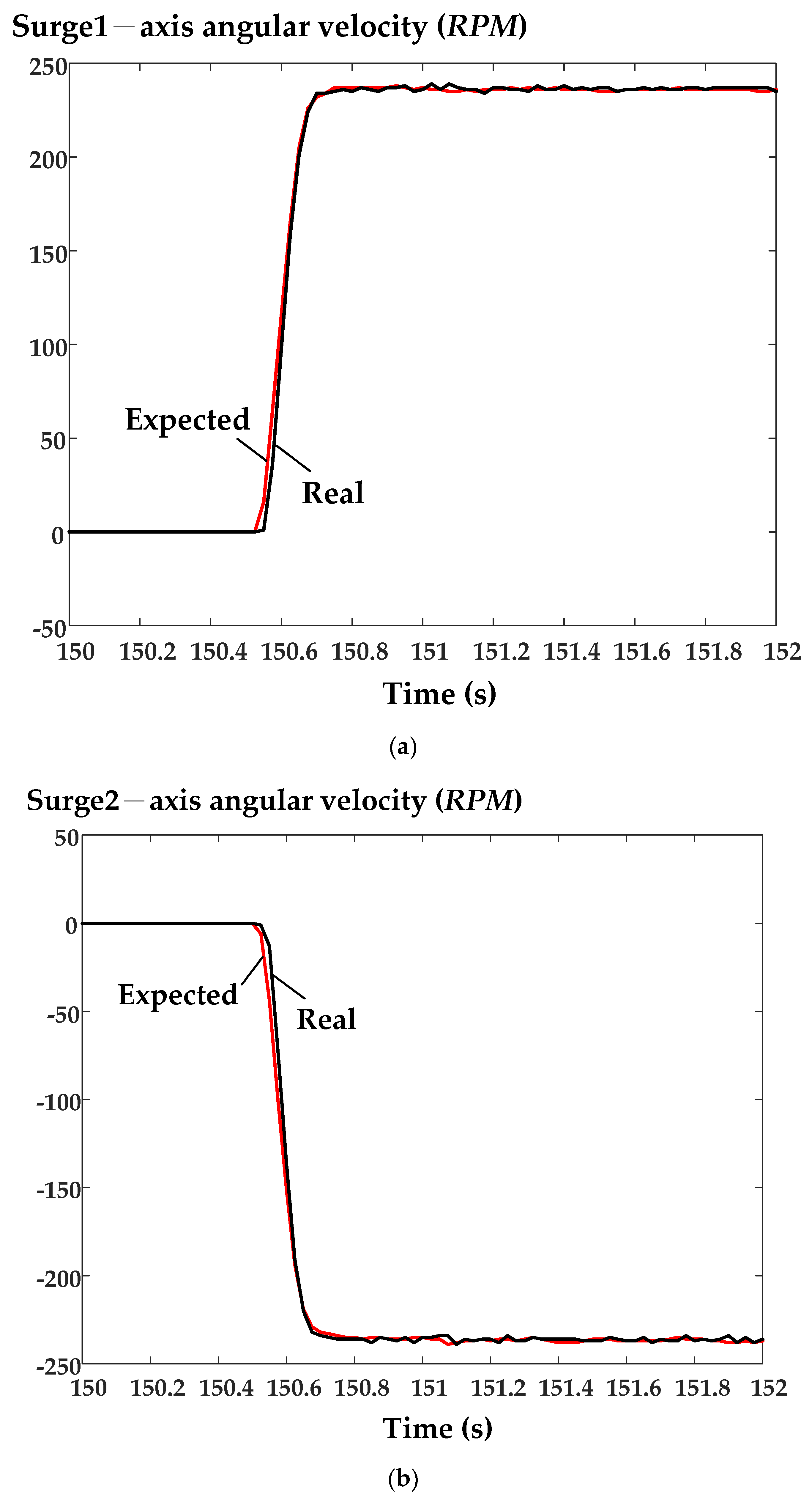
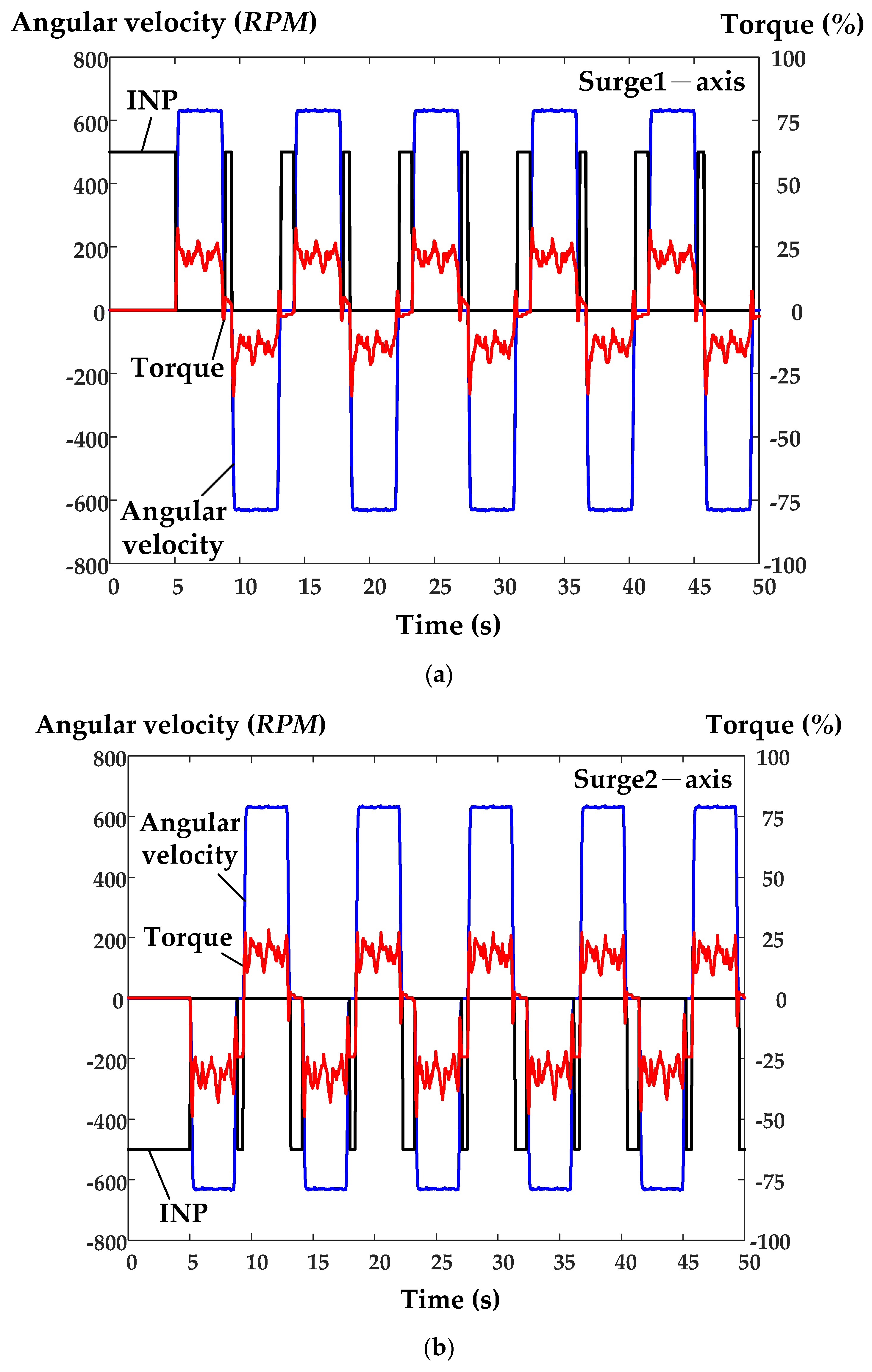
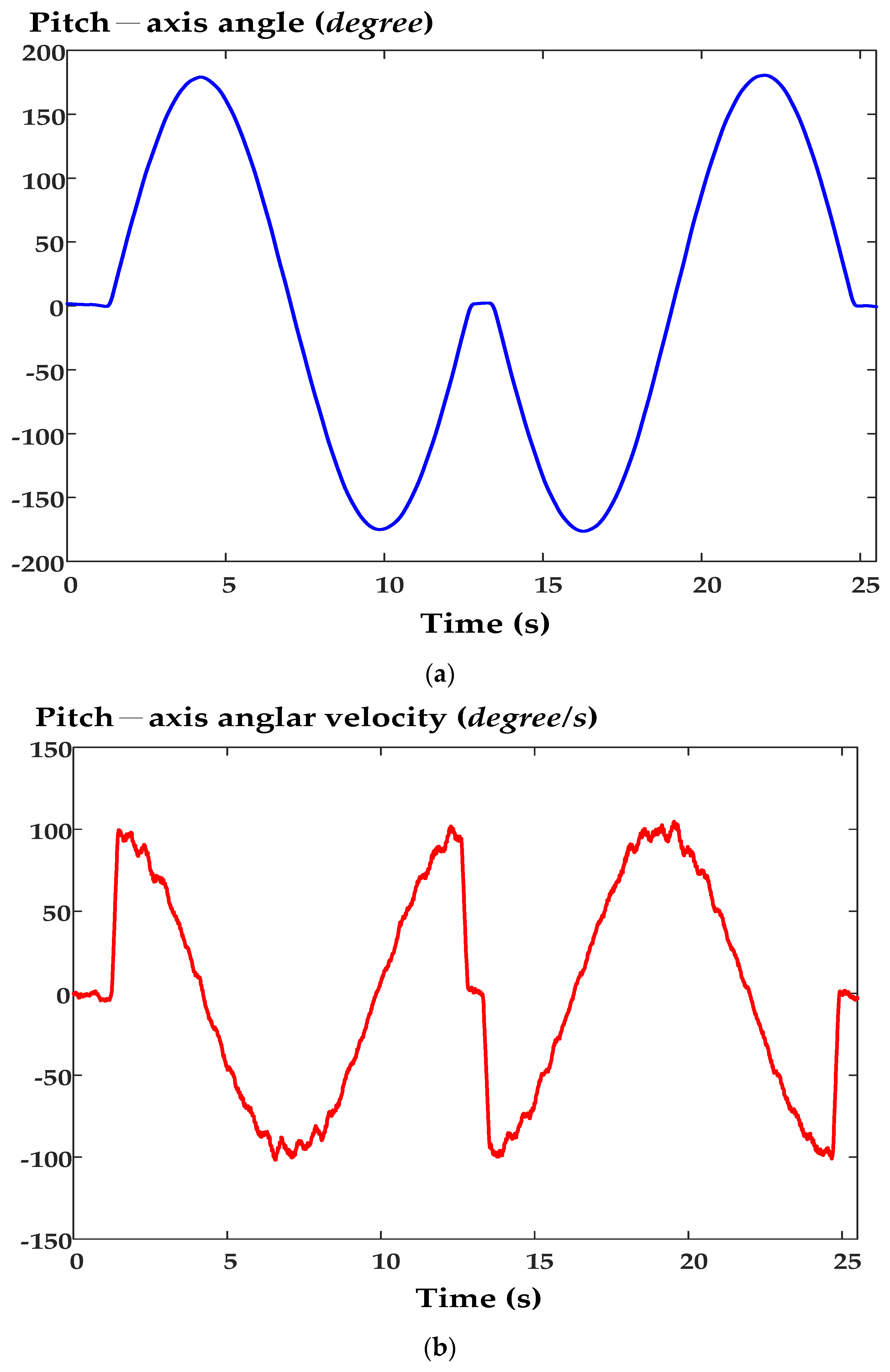
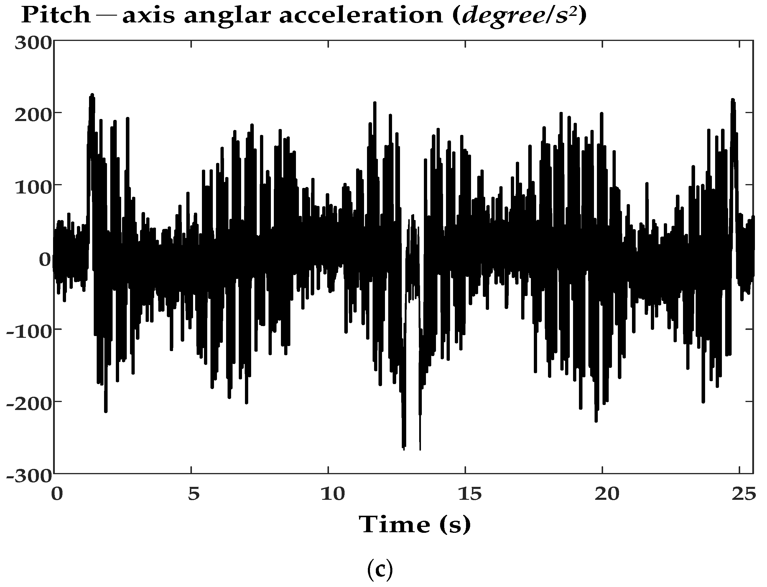
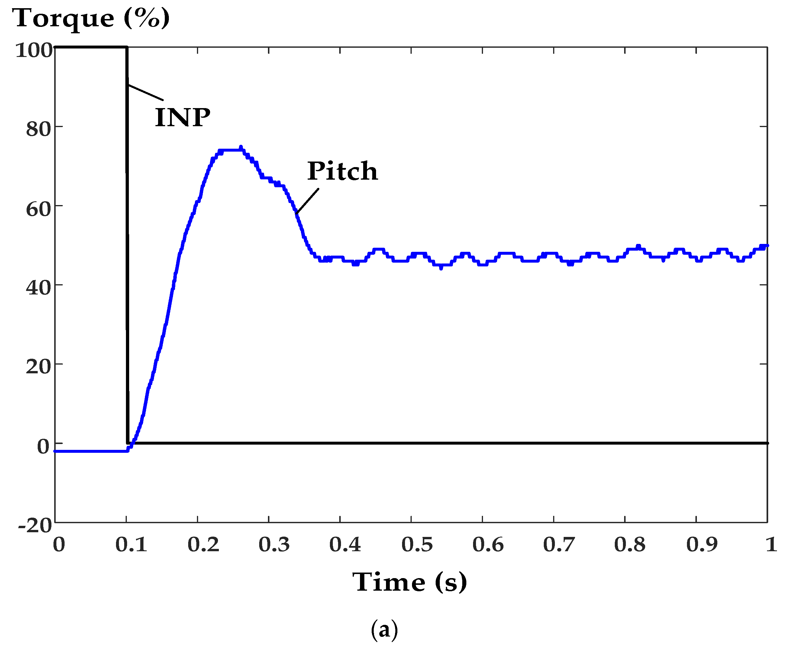
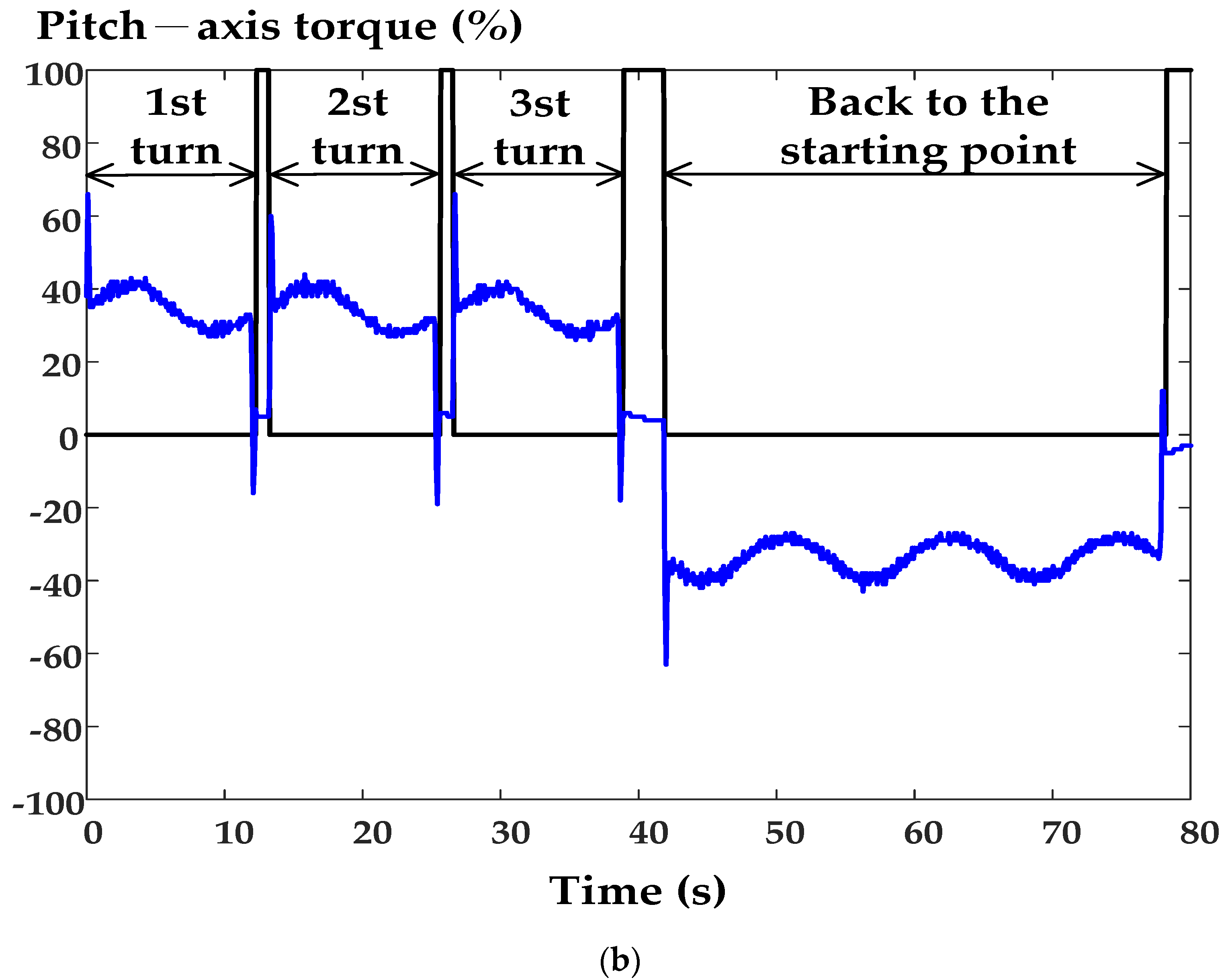
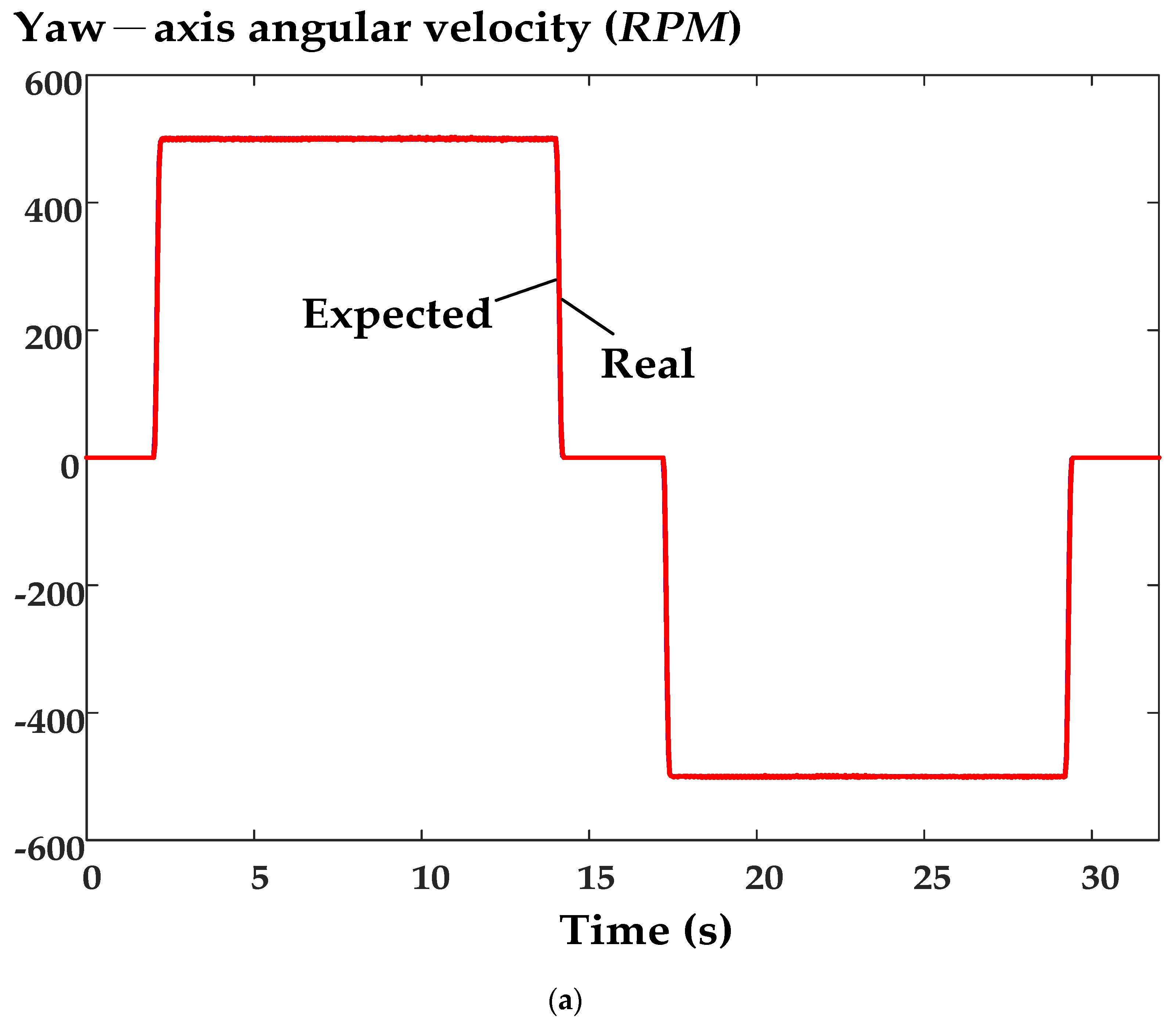
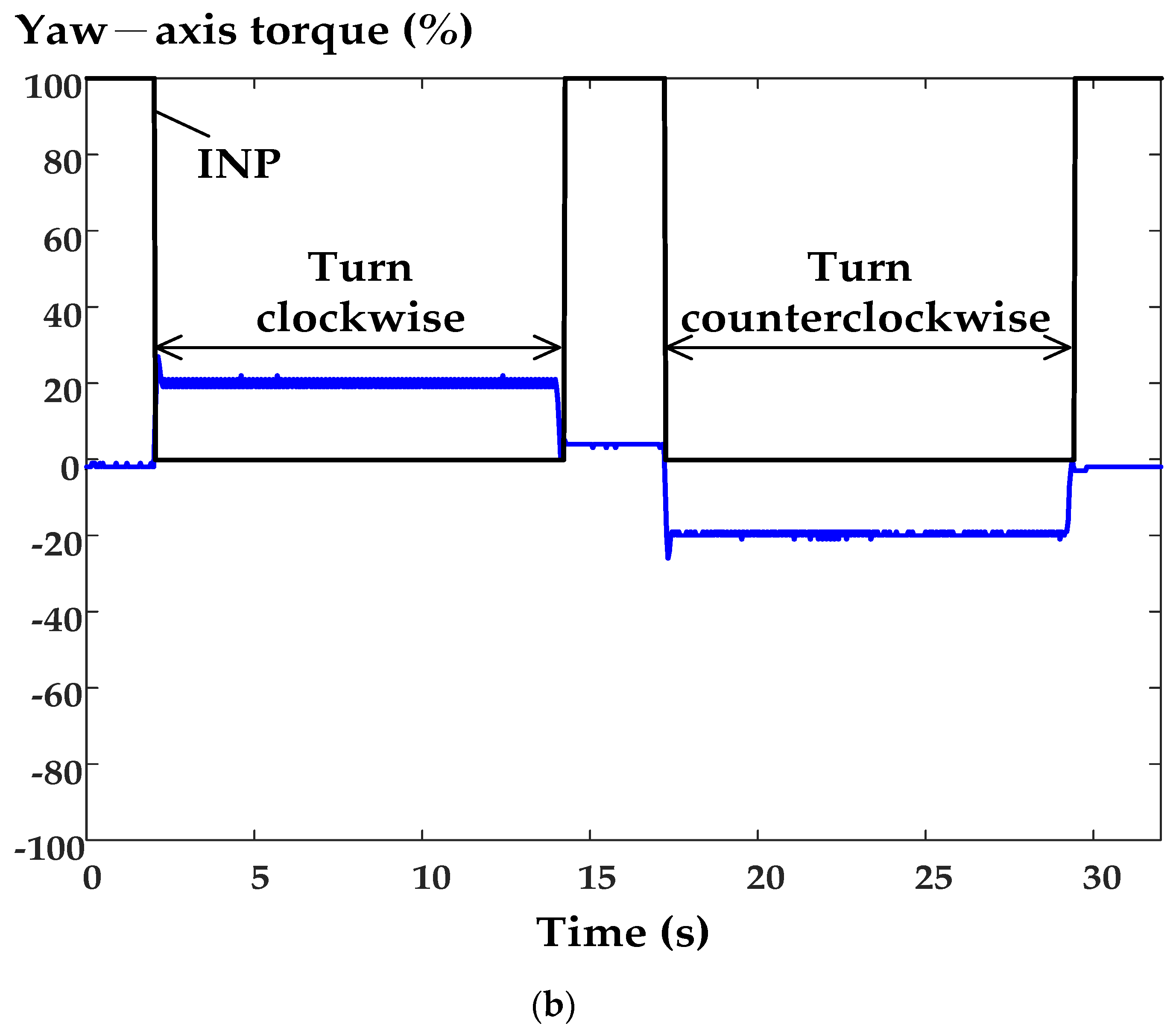
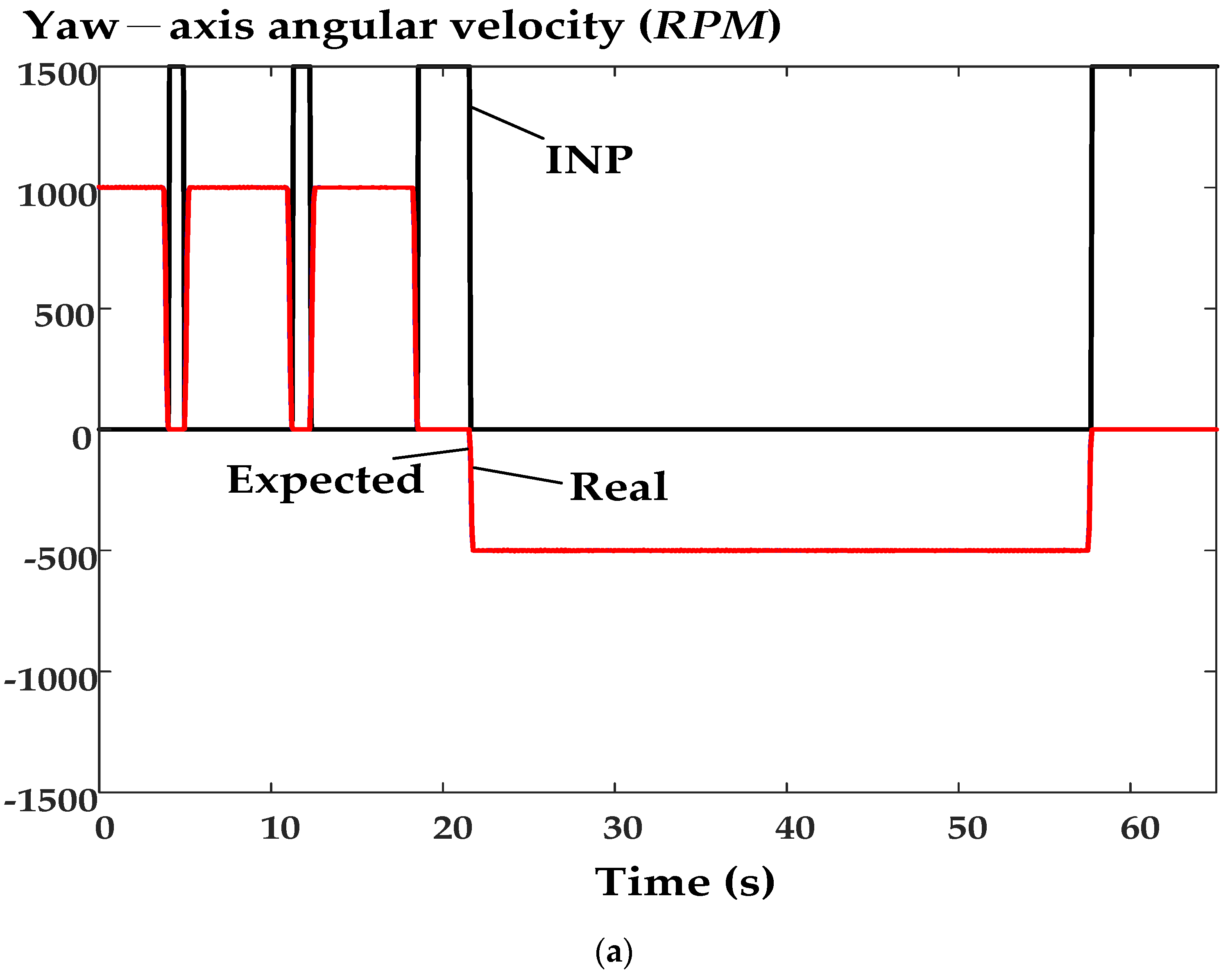
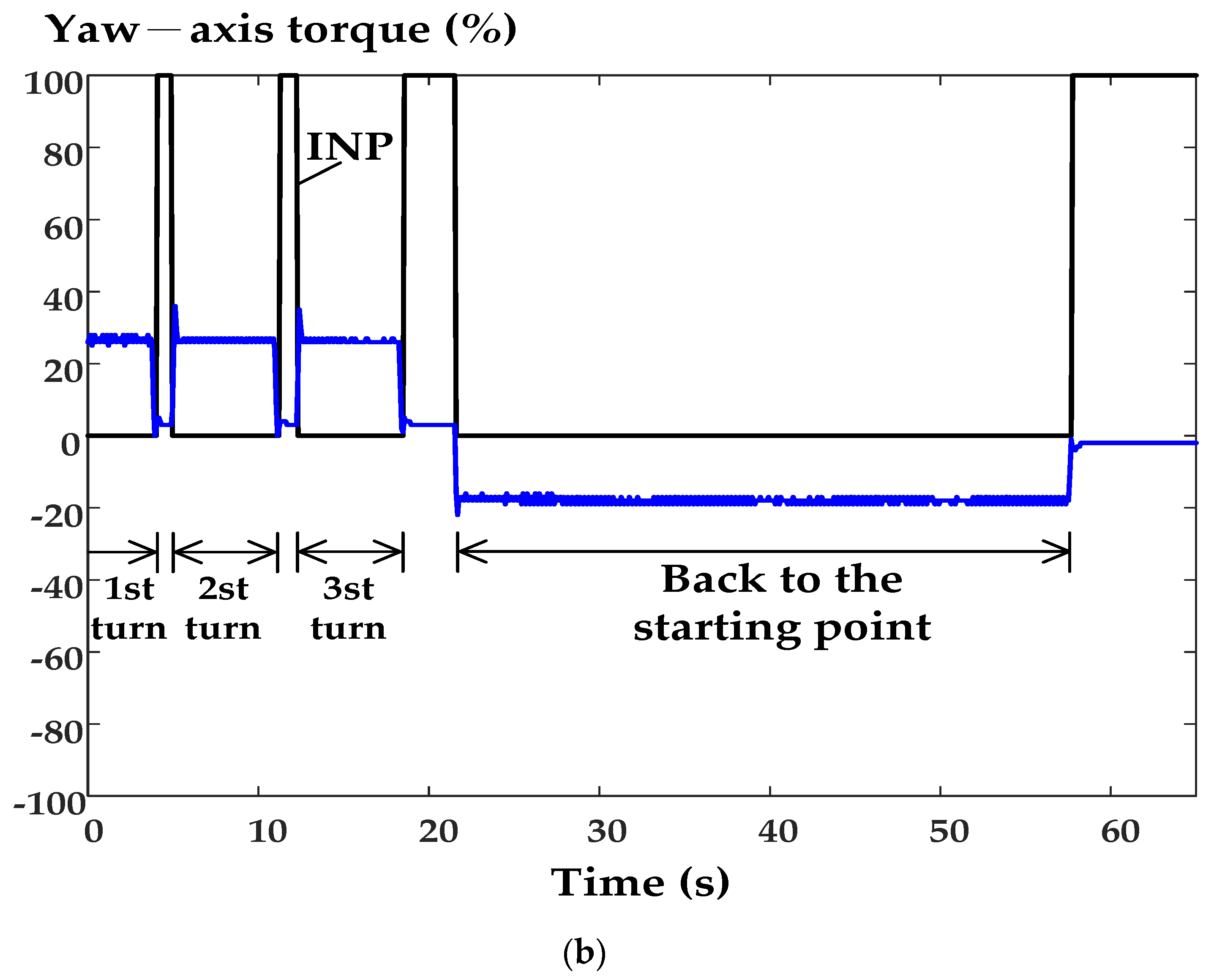
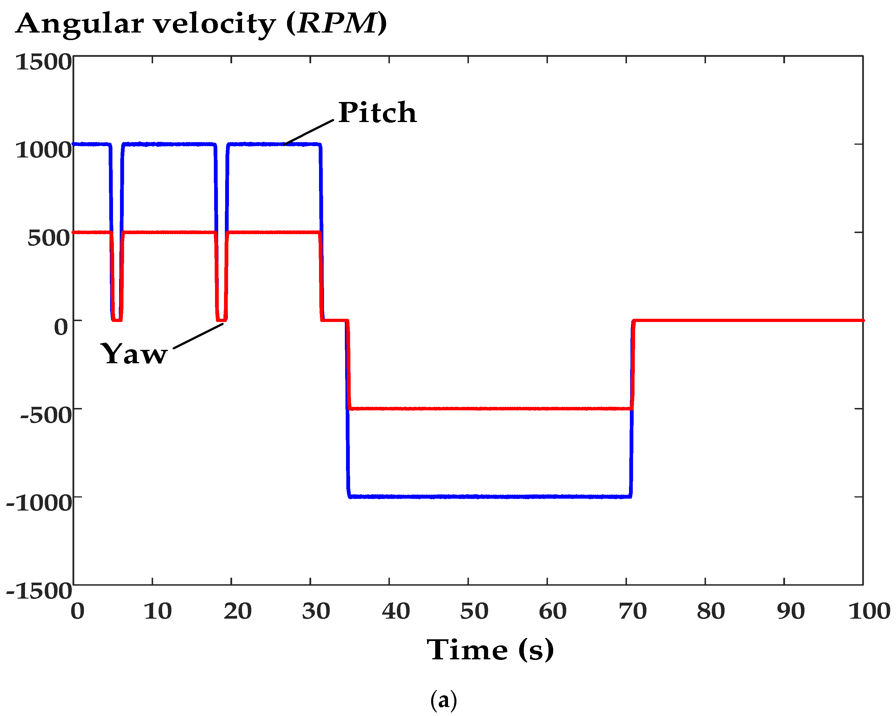
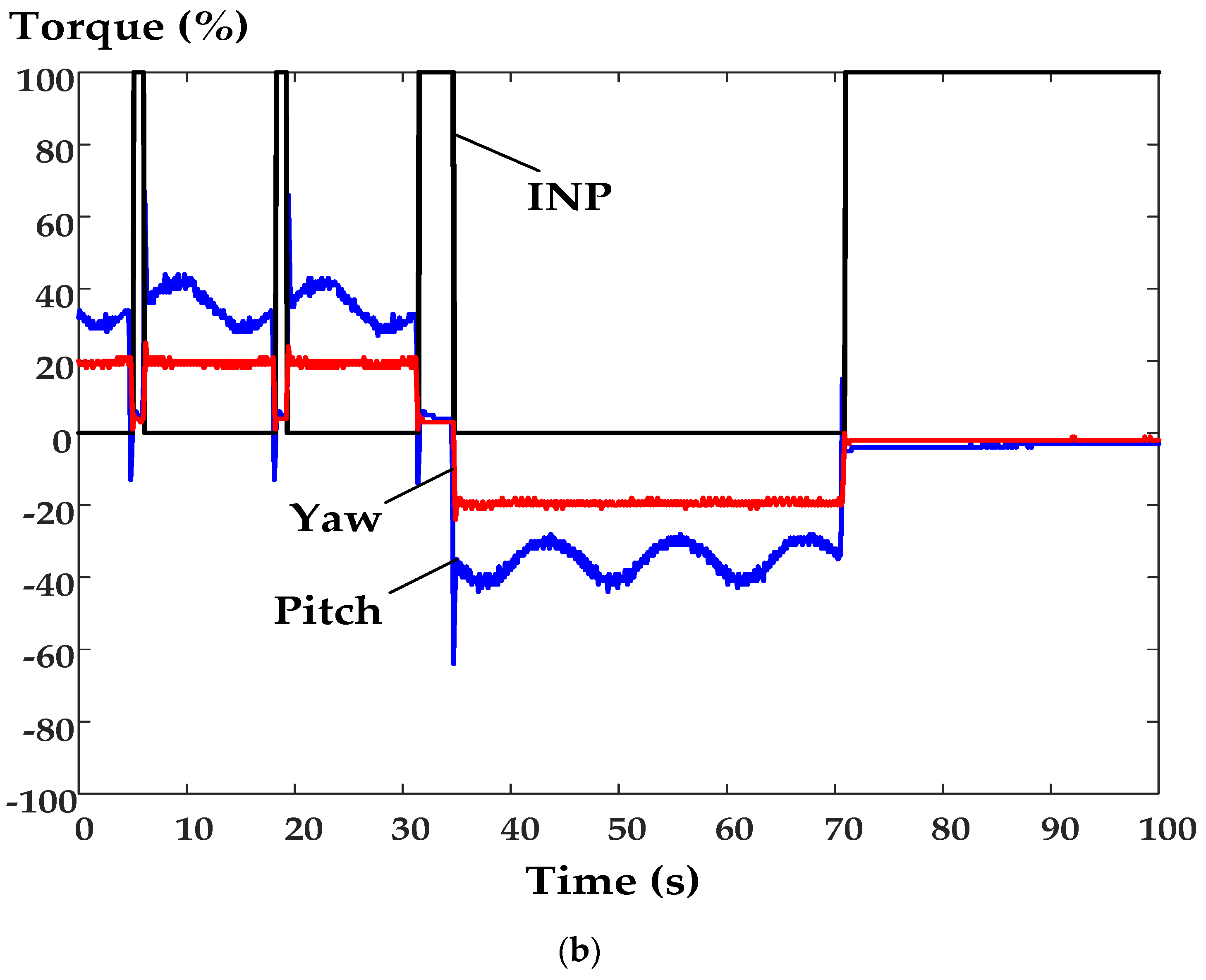
The test process is to issue platform commands to the platform through the user interface, and the driver records the relevant real measurement results, as shown in Figure 13, Figure 14, Figure 15, Figure 16, Figure 17, Figure 18, Figure 19, Figure 20, Figure 21, Figure 22, Figure 23, Figure 24, Figure 25 and Figure 26. The development of the verification platform discussed in this paper is divided into a platform, power box, and control box, as shown in Figure 10a,b. The control box adopts the digital signal processor board as the control core design. Considering the installation space, convenience, and writing software factors, it adopts a three-degree-of-freedom (surge axis, pitch axis, and yaw axis) design, as shown in Figure 11. In this paper, the CAN bus protocol is implemented using the CAN2.0A basic data format, which consists of an 11-bit identifier and data bytes for each message. The ability of the CAN bus protocol to detect and recover from transmission errors is a crucial feature for ensuring reliable communication in industrial systems. The transmission packets of the five digital signal processors used in the system are illustrated in Figure 13, with the CAN_H signal driven high and the CAN_L signal driven low, resulting in a potential difference between the two signals. The addition of 120 Ω termination resistors at each end of the CAN bus network and the use of a shielded twisted pair bus cable help to improve the reliability of CAN communication. The specific CAN message identification used in the system is illustrated in Figure 14. Figure 14a–d display the signals for ID = 0xA1~0xA8 of the main control board, denoted as #0, as well as the corresponding signals for the four slave control boards (#1~#4) with respective IDs of 0x11~0x14, 0x21~0x24, 0x31~0x34, and 0x41~0x44. These explanations allow readers to have a clearer comprehension of the system’s architecture and emphasize the pivotal role of implementing the CAN bus protocol, along with the associated hardware and software, to ensure reliable and robust communication in industrial environments. Proper implementation of the CAN bus protocol and its associated hardware and software is crucial for ensuring reliable and robust communication in the system. The CAN bus protocol is widely used in industrial applications because of its high reliability, low cost, and efficient message transfer. Figure 15a,b are the angle response of the low-accuracy encoder and the high-accuracy encoder, respectively. It can be seen that the signals of the two vary between −180 and 180 degrees, and 2 encoders can be seen from the observation figure. The angle changes under motor driving are consistent, which means that the proposed motor calibration platform can drive the two encoders smoothly. Figure 15c is a comparison between the two. It can be seen from the figure that when the time axis is enlarged to 0.1 s, there is a slight angle error in the low-accuracy encoder. The reason for this is that a 50 arc-second encoder is used to perform digital calibration, compared to a 5 arc-second high-precision encoder, and there is a significant difference in specifications. For further analysis and comparison, the vertical axis is changed to the number of errors between the two encoders, and the horizontal axis uses the low-accuracy encoder angle as a reference value, as shown in Figure 16a,b. Figure 16a is the error response diagram of the method proposed in this paper. It is obvious from the diagram that there is an error offset in the encoder, and its maximum error is about 0.034 degrees. For the working conditions with high-accuracy requirements, it is relatively unable to meet the needs of the system. Observing Figure 16b, it can be clearly seen that after the digital calibration platform proposed in this paper, the number of errors will be effectively reduced to ±0.004 degrees, indicating that the proposed method can be used to improve the accuracy of the encoder angle. The test process is to issue platform commands to the platform through the user interface and record the relevant measurement results using the measurement software and the driver, as shown in Figure 17, Figure 18, Figure 19, Figure 20, Figure 21, Figure 22, Figure 23, Figure 24, Figure 25 and Figure 26. Figure 17a,b show the torque utilization rate when the surge axis servo is enabled, and Figure 17a shows it at rest. The surge1 and surge2 real axes are meshed by spur racks and spur gears. Since the surge1 and surge2 servo and deceleration mechanisms are placed in relative positions, the linear drive capability of the surge axis is improved. It can be seen from the figure that the motor output is −8% and −3%; at rest, the two are about the same. Figure 17b is the response graph at the moment of starting. It can be seen that the torque command will change with the acceleration process due to the need to overcome the static friction force and the meshing gear to drive the upper platform during start-up. Figure 18a–c are the displacement, velocity, and acceleration of the surge axis moving 0–500 mm. Figure 18b shows that the maximum speed is 500 mm/s. The acceleration is 2000 mm/s. Figure 19a,b are a comparison diagram of bilateral drive. It can be seen that due to the relative position placement, when the platform is driven linearly from 0 to 500 mm in 1 s and 500 to 0 mm in 5 s, it is determined by the angular velocity. The figure shows that the speed and torque on both sides are opposites. Figure 20a,b are the speed comparison diagram of bilateral drive. The red line is the speed command calculated by the driver through the position controller, and the black line is the real speed. It can be seen that the speed command and the real speed are temporarily at 150.5–150.6 s. The state is slightly behind due to the influence of the platform load. When the speed increases and the controller adjustment is completed, the speed command can be tracked. Figure 21a is a comparison diagram of the speed and torque response during the motion control of the surge1 axis. The black line (INP) is the level judgment of the positioning completion. It can be seen that repeated positioning can be achieved in five times of control. Figure 21b is a comparison diagram of the speed and torque commands of the surge2 axis, and the black line is the level judgment of the positioning completion. From Figure 21a,b, it can be seen that the bilateral linear drive has good stability characteristics before and after reciprocation. Figure 17, Figure 18, Figure 19, Figure 20 and Figure 21 show that the proposed linear transmission and servo drive architecture can meet the requirements for the linear drive capability of the six-axis rolling platform and at the same time use the bilateral drive method to improve the output and drive smoothness. Figure 22a–c are the angle, angular velocity, and acceleration of the ±180-degree rotation of the pitch axis. Figure 22b shows that the maximum speed is 100 degrees/s. The acceleration is 200 degrees/s. Figure 23a,b are the torque command response diagram of the pitch axis drive starting and continuous rolling. Figure 23a shows that the maximum transient output of the pitch axis is about 75%, and the steady-state torque utilization rate is 50%. Figure 23b is the torque characteristic of testing continuous rolling. In the interval of 0–40 s, it will stop for 1 s after each positive rotation and then roll the second rotation until the test is intermittent and continuous, known as the rolling effect. When the rolling is finished, the back-to-origin test is used to determine the effect of rolling three times in a row. Figure 24a,b are the real measurement result of the yaw axis driving the turntable in the turntable to rotate once through the collector slip ring. Figure 24a is the angular velocity response. It can be seen there that the motor speed range is ±500 rpm. Figure 24b is the angular velocity response. It can be seen there that the torque range is ±20%. Figure 25a,b show the real measurement results of the yaw axis driving the turntable to rotate three times through the collector slip ring. Similarly, in the interval of 0–18 s, it will stop for one second after each positive turn and then roll the second turn until the full three weights are used to test the intermittent continuous rolling effect. Figure 25a is the angular velocity response. It can be seen there that the maximum positive speed range of the motor is about +1000 rpm, and the maximum rich speed is about −500 rpm. Figure 25b is the angular velocity response. It can be seen there that the torque range is ±25%. Comparing the torque response in Figure 24b and Figure 25b, it can be determined that the power transmitted to the servo motor by the number of rings of the power line of the collector slip ring is stable. When the current value is normal, the torque transient and steady state will show a continuous phenomenon. Figure 26a,b show the measure response of angular velocity and torque. The real motion response characteristics of the pitch axis and yaw axis velocity can be determined through Figure 22, Figure 23, Figure 24, Figure 25 and Figure 26.

Table 2. The measurement results.

	DOF	Surge1	Surge2	Pitch	Yaw
Item
Stroke		500 mm	500 mm	360°	360°
Velocity		>500 mm/s	>500 mm/s	>30°/s	>60°/s
Acceleration		>2000 mm/s2	>2000 mm/s2	>30°/s2	>60°/s2
Actual motor torque		>25%	>25%	>40%	>20%
Axis load weights		190 Kg	190 Kg	100 Kg	15.4 Kg
Communication		CAN bus and RS485	CAN bus and RS485	CAN bus and RS485	CAN bus and RS485

shows the measurement results.

7. Conclusions

This paper presents the design and control of a three-degree-of-freedom motion system using a digital architecture consisting of a master and four slaves, with data handshaking achieved through the CAN bus communication transmission interface. The digital control system allows for the user interface and overall motion system to be achieved digitally, eliminating the shortcomings of traditional systems and improving the entire industry. The proposed system can be applied to more complex control technologies and includes features such as a digital encoder accuracy adjustment method, motion path planning, motion system structural design, servo drive technology, and mathematical model establishment. An experimental platform with mathematical derivation, three-axis control, and combined software/hardware control methods was developed and analyzed to verify the structural assembly for production. The proposed three-axis motion platform showed good experimental results, including long-distance travel and continuous rotation effects. The motion system was realized using PID controllers, which are still widely used in related industrial control fields because of their strong robustness, good stability, and simple structure. Although the study did not focus primarily on the modern control theory of the platform, future studies will consider it to assess the design and enhance its capabilities. Moreover, the proposed three-axis motion servo control system based on a CAN bus can also be adapted for innovative manipulator layouts [33,34]. Subsequently, future studies will explore the modern control theory of the platform to further evaluate its design and enhance its performance and capabilities across various applications.

References

- Lu, H.; Cheng, Q.; Zhang, X.; Liu, Q.; Qiao, Y.; Zhang, Y. A novel geometric error compensation method for gantry-moving CNC machine regarding dominant errors. Processes 2020, 8, 906. [Google Scholar] [CrossRef]
- Martinov, G.M.; Al Khoury, A.; Issa, A. An approach of developing low cost ARM based CNC systems by controlling CAN drive. In Proceedings of the International Conference on Modern Trends in Manufacturing Technologies and Equipment (ICMTMTE 2018), Sevastopol, Russia, 10–14 September 2018; pp. 1–6. [Google Scholar]
- Babici, L.M.; Tudor, A.; Romeu, J. Stick-Slip Phenomena and Acoustic Emission in the Hertzian Linear Contact. Appl. Sci. 2022, 12, 9527. [Google Scholar] [CrossRef]
- Uchimura, Y.; Yakoh, T. Bilateral robot system on the real-time network structure. IEEE Trans. Ind. Electron. 2004, 51, 940–946. [Google Scholar] [CrossRef]
- Ferrel, W.R. Remote manipulation with transmission delay. IEEE Trans. Human Factors Electron. 1965, 6, 24–32. [Google Scholar] [CrossRef]
- Smith, O.J. A controller to overcome dead time. ISA J. 1959, 6, 28–33. [Google Scholar]
- Anderson, R.J.; Spong, M.W. Bilateral control of teleoperators with time delay. IEEE Trans. Automat. Contr. 1989, 34, 494–501. [Google Scholar] [CrossRef]
- Leung, G.; Francis, B.; Apkarian, J. Bilateral controller for teleoperators with time delay via –synthesis. IEEE Trans. Robot. Automat. 1997, 11, 105–116. [Google Scholar] [CrossRef]
- Zhao, H.; Wang, S.; Liu, Y.; Zhu, J. Control and communication of a multi-motor system based on LAN. J. Inf. Commun. Eng. 2016, 2, 94–98. [Google Scholar]
- Available online: https://en.wikipedia.org/wiki/CAN_bus (accessed on 24 March 2023).
- Deng, R.; Wang, Y. Design and preliminary implementation of distributed control system for pipeline detection serpentine robot based on CAN bus. In Proceedings of the International Conference on Chinese Automation Congress (CAC 2019), Hangzhou, China, 22–24 November 2019; pp. 3124–3128. [Google Scholar]
- Torres, G.; Velasco, M.; Marti, P.; Fuertes, J.M. An alternative discrete time model for networked control systems with time delay less than the sampling period. In Proceedings of the Annual Conference of the IEEE Industrial Electronics Society (IECON 2013), Vienna, Austria, 10–13 November 2013; pp. 5626–5631. [Google Scholar]
- Yang, R.; Liu, G.P.; Shi, P.; Thomas, C.; Basin, M.V. Predictive output feedback control for networked control systems. IEEE Trans. Ind. Electron. 2014, 61, 512–520. [Google Scholar] [CrossRef]
- Herpel, T.; Hielscher, K.S.; Klehmet, U.; German, R. Stochastic and deterministic performance evaluation of automotive CAN communication. Comput. Netw. 2009, 53, 1171–1185. [Google Scholar] [CrossRef]
- Wei, M.Y. Design and Implementation of Inverse Kinematics and Motion Monitoring System for 6DoF Platform. Appl. Sci. 2021, 11, 9330. [Google Scholar] [CrossRef]
- Wei, M.Y. Design of a DSP-based motion-cueing algorithm using the kinematic solution for the 6-DoF motion platform. Aerospace 2022, 9, 203. [Google Scholar] [CrossRef]
- Gough, V.E. Practical tire research. SAE Trans. 1956, 64, 310–318. [Google Scholar]
- Stewart, D. A platform with six degrees of freedom. Proc. Inst. Mech. Eng. 1965, 180, 371–386. [Google Scholar] [CrossRef]
- Lara-Molina, F.A.; Rosario, J.M.; Dumur, D. Architecture of predictive control for a Stewart platform manipulator. In Proceedings of the International Conference on World Congress on Intelligent Control and Automation (WCICA 2010), Jinan, China, 7–9 July 2010; pp. 6584–6589. [Google Scholar]
- Bruschetta, M.; Maran, F.; Beghi, A. A Nonlinear, MPC-based motion cueing algorithm for a high-performance, nine-DoF dynamic simulator platform. IEEE Trans. Control Syst. Technol. 2017, 25, 686–694. [Google Scholar] [CrossRef]
- Asadi, H.; Mohammadi, A.; Mohamed, S.; Qazani, M.R.C.; Lim, C.P.; Khosravi, A.; Nahavandi, S. A model predictive control-based motion cueing algorithm using an optimized nonlinear scaling for driving simulators. In Proceedings of the International Conference on Systems, Man and Cybernetics (SMC), Bari, Italy, 6–9 October 2019; pp. 1245–1250. [Google Scholar]
- Mohammed, A.M.; Li, S. Dynamic neural networks for kinematic redundancy resolution of parallel Stewart platforms. IEEE Trans. Cybern. 2016, 46, 1538–1550. [Google Scholar] [CrossRef]
- Tang, Z.; Hu, M.; Pei, Z.; Liu, L.; Zhang, J. A new numerical method for Stewart platform forward kinematics. In Proceedings of the International Conference on Chinese Control Conference (CCC), Chengdu, China, 27–29 July 2016; pp. 6311–6316. [Google Scholar]
- Lou, J.H.; Tseng, S.P. Developing a real-time serial servo motion control system for electric Stewart platform. In Proceedings of the International Conference on Advanced Robotics and Intelligent Systems (ARIS), Taipei, Taiwan, 6–8 June 2014; pp. 66–71. [Google Scholar]
- Qazani, M.R.C.; Asadi, H.; Khoo, S.; Nahavandi, S. A linear time-varying model predictive control-based motion cueing algorithm for hexapod simulation-based motion platform. IEEE Trans. Syst. Man, Cybern. 2021, 51, 6096–6110. [Google Scholar] [CrossRef]
- Asadi, H.; Lim, C.P.; Mohamed, S.; Nahavandi, D.; Nahavandi, S. Increasing motion fidelity in driving simulators using a fuzzy-based washout filter. IEEE Trans. Intell. Veh. 2019, 4, 298–308. [Google Scholar] [CrossRef]
- Wei, M.Y.; Yeh, Y.L.; Liu, J.W.; Wu, H.M. Design and control of a multi-axis servo motion chair system based on a microcontroller. Energies 2022, 15, 4401. [Google Scholar] [CrossRef]
- Shukla, H.; Roy, S.; Gupta, S. Robust adaptive control of steer-by-wire systems under unknown state-dependent uncertainties. Int. J. Adapt. Control. Signal Process. 2022, 36, 198–208. [Google Scholar] [CrossRef]
- Yadav, R.D.; Sankaranarayanan, V.N.; Roy, S. Adaptive sliding mode control for autonomous vehicle platoon under unknown friction forces. In Proceeding of the International Conference on Advanced Robotics (ICAR 2021), Ljubljana, Slovenia, 6–10 December 2021; pp. 879–884. [Google Scholar]
- Rayguru, M.M.; Mohan, R.E.; Parween, R.; Yi, L.; Le, A.V.; Roy, S. An Output Feedback Based Robust Saturated Controller Design for Pavement Sweeping Self-Reconfigurable Robot. IEEE/ASME Trans. Mechatron. 2021, 26, 1236–1247. [Google Scholar] [CrossRef]
- Liu, T.H.; Lu, W.R.; Cheng, S.H. Design and implementation of predictive controllers for a 36-slot 12-pole outer-rotor SPMSM/SPMSG system with energy recovery. Energies 2023, 16, 2845. [Google Scholar] [CrossRef]
- AI-Mualla, M.E.; Canagarajah, N.; Bull, D.R. Error concealment using motion field interpolation. In Proceedings of the International Conference on Image Processing (ICIP 98), Chicago, Il, USA, 7 October 1998; pp. 512–516. [Google Scholar]
- Fiorineschi, L.; Pugi, L.; Rotini, F. New mechanism for press-fit processes: Preliminary analysis. World J. Eng. 2023, 20, 1–11. [Google Scholar] [CrossRef]
- Ducci, M.; Peruzzi, A.; Pugi, L. Impact of combined roto-linear drives on the design of packaging systems: Some applications. In Proceedings of the International Conference on Applications in Electronics Pervading Industry, Environment and Society; Springer: New York, NY, USA, 2021; Volume 738, pp. 235–240. [Google Scholar]
Figure 1.
Three-degree-of-freedom motion platform.
Figure 2.
The relationship in the surge axis between the bilateral real axes and virtual axis.
Figure 3.
Multi-axis motion control architecture diagram.
Figure 4.
Block diagram of the servo control system.
Figure 5.
Flowchart of encoder measurement accuracy.
Figure 6.
Flowchart of the proposed encoder error compensation method.
Figure 7.
Monitoring system: (a) photograph, (b) laser displacement meter, and (c) operator interface.
Figure 8.
The block diagram of the 3-DOF platform.
Figure 9.
A 3D design drawing of the 3-DOF platform.
Figure 10.
The implemented system: (a) power box and (b) control box.
Figure 11.
The implementation system: photo of (a) the motion platform, (b) monitoring system, and (c) the inside of the rotating cabin.
Figure 12.
Flowchart of motion control implementation.
Figure 13.
CAN bus signal (Top: CAN_H signal, Bottom: CAN_L signal).
Figure 14.
DSP (TMS320F28377) #0: (a) 0xA1~0xA3; (b) 0xA4~0xA5; (c) 0xA6~0xA7; (d) 0xA8.
Figure 15.
The encoder angle response diagram when the motor is forward and reverse: (a) low-accuracy encoder; (b) high- accuracy encoder; (c) comparison of two encoders at different angles.
Figure 16.
The horizontal axis is the angle of the low-accuracy encoder, and the vertical axis is the error of the two encoders: (a) without calibration; (b) after calibration.
Figure 17.
Measured torque responses of the surge axis: (a) standstill; (b) starting.
Figure 18.
Measured responses at square-wave position command of the surge axis: (a) displacement; (b) velocity; (c) acceleration.
Figure 19.
Measured responses of the bilateral drive of the motors with the surge1 and surge2 axis displacement of 500 mm: (a) angular velocity; (b) torque.
Figure 20.
Measured responses of a square-wave speed command: (a) surge1; (b) surge2.
Figure 21.
Measured responses of the motors for 5 times of surge axis displacements of 0–500 mm: (a) surge1; (b) surge2.
Figure 22.
Measured responses of pitch axis angle command: (a) angle; (b) angular velocity; (c) angular acceleration.
Figure 23.
Measured torque responses of the pitch axis: (a) starting; (b) turn three times and return to the original angle.
Figure 24.
Measured responses of the motor with the yaw axis angle of 360 degrees: (a) angular velocity; (b) torque.
Figure 25.
Measured responses of the motor for three revolutions of the yaw axis angle of 360 degrees: (a) angular velocity; (b) torque.
Figure 26.
Measured responses of the motors of the pitch axis and yaw axis: (a) angular velocity; (b) torque.