Optimal Capacity and Operational Planning for Renewable Energy-Based Microgrid Considering Different Demand-Side Management Strategies

Abstract

A bi-objective joint optimization planning approach that combines component sizing and short-term operational planning into a single model with demand response strategies to realize a techno-economically feasible renewable energy-based microgrid is discussed in this paper. The system model includes a photovoltaic system, wind turbine, and battery. An enhanced demand response program with dynamic pricing devised based on instantaneous imbalances between surplus, deficit, and the battery’s power capacity is developed. A quantitative metric for assessing energy storage performance is also proposed and utilized. Emergency, critical peak pricing, and power capacity-based dynamic pricing (PCDP) demand response programs (DRPs) are comparatively analyzed to determine the most cost-effective planning approach. Four simulation scenarios to determine the most techno-economic planning approach are formulated and solved using a mixed-integer linear programming algorithm optimization solver with the epsilon constraint method in Matlab. The objective function is to minimize the total annualized costs (TACs) while satisfying the reliability criterion regarding the loss of power supply probability and energy storage dependency. The results show that including the DRP resulted in a significant reduction in TACs and system component capacities. The cost-benefit of incorporating PCDP DRP strategies in the planning model increases the overall system flexibility.

1. Introduction

The electric power system is experiencing tremendous transformation globally to meet the rising electricity demand and combat greenhouse emissions. Due to its low operational costs and emission-free nature, adopting renewable energy has been crucial for achieving carbon neutrality in electric power grids. Variable renewable energy sources (VREs), mainly wind and solar, currently comprise most of the world’s electricity sources due to their abundant resource potential and local availability [1,2]. However, due to their intrinsic variability, the widespread incorporation of VREs has imposed massive complexity in the power systems’ capacity sizing and operational planning [3]. With the limited capacity of the ESS to smoothen out the surplus or deficient power in the energy system, it is complicated to balance power demand and supply at high-time resolutions. Due to VREs’ limited dispatchability, the need to improve the power system planning approaches and incorporate more flexible resources and technologies to enhance system elasticity and flexibility is becoming increasingly important [4]. Flexibility is the power system’s capacity to balance electricity supply and demand when highly variable energy resources are incorporated [5]. Notably, ESS provides the necessary temporal support to offset the variabilities of VRE, and dispatchable power plants a quick ramping up generation supplement in times of low wind and solar [6]. The transmission networks offer geographical smoothing to balance the supply and demand in the system [7,8]. Demand-side management strategies regulate the FDRs to address the mismatch between the load demand and power output of the VREs [9]. Thus, including demand response strategies in a joint long-term component sizing and operation planning model is essential to realize a high VREs-based power system.

The recent innovative grid concept has injected more intelligence into grid management practices, especially in the face of changing load patterns and the proliferation of energy supply from renewable energy injection [10]. Thus, existing grid infrastructures are well equipped with information and communication technologies for real-time monitoring and prompt control of power system equipment. As a result, the incorporation of smartness into grid infrastructures is now making the concept of demand-side management (DSM) a vital component of the electricity infrastructures of many nations all over the world [11]. While DSM is a broad concept, demand response programs (DRP) are underlying energy market strategies whereby consumers’ electricity consumption behaviors are tactically altered regarding the time of demand for using their flexible loads [12]. The specific goal of demand-side management is to ensure that the most suitable and economically viable operating conditions are achieved based on the information on the available supply (generating) capacity, the demand (load) requirements, and the energy market dynamics per time. Thus, specific changes in customers’ electricity usage patterns are achieved by utility companies providing some incentivization through friendly tariff packages such as flexible payments and lucrative prices for altered load demand patterns and the consequently consumed electricity units. With an appropriately designed DRP scheme, the effective grid planning and operation cost resulting from additional generation and transmission capacity expansion towards meeting increased load demand can be grossly reduced [13]. Fundamentally, existing DRP models can be classified as either rate/price-based or incentive/event-based demand response models under which there are different DRP types, namely day-ahead pricing (DHP), critical peak pricing (CPP), time of use (TOU), real-time pricing (RTP), etc. [14,15].

Demand response programs (DRPs) are a crucial enabling framework in maintaining the power grid’s reliability and stability through electricity market participation. DRP operation strategies provide a mechanism for controlling or rescheduling flexible power demands to increase or decrease capacity during specific periods, for example, to take advantage of high VRE generation or lessen peak demand in the system [16]. As mentioned above, these techniques make it possible to incorporate large amounts of VREs into the power network in the most economical way possible [17]. Depending on the motivation strategies of the DRP adopted, the subscribed customers (both residential [18] and industrial [19]) are enticed to regulate the power consumption of their flexible demand resource when the total power generation is insufficient and vice versa. Through rebates or incentive payments, consumers are rewarded for reducing their peak demands or shifting part of their daily energy consumption from peak to off-peak hours. As substantiated in numerous literature, the most efficient approach to implementing an effective DRP is that it influences most consumers to participate in real-time power-dispatching transactions, ensuring that the system’s overall efficiency and stability are improved [20]. The DRPs have numerous potential benefits in all aspects of power system planning, i.e., operation planning [21] and long-term capacity and expansion planning [22]. By implementing a well-devised DRP to utilize the installed capacity optimally, it is possible to postpone investing in additional new generating units, delay non-essential network upgrades, etc. Hence, it is essential to incorporate DRP strategies into the operation and capacity planning models. Moreover, implementing suitable demand response (DR) programs and load shifting techniques can enhance the technical performances of energy system networks towards resolving potential overvoltage issues in the network [23].

Many economic and technical power system planning studies in the literature consider multi-stage or segregated planning models: long-term investment models as well as operation or unit commitment models to determine the optimal operation planning and demand side management to determine the best electricity market operation strategies with varied simulation time frames [24]. At the long-term investment level, the planning model specifically handles the capacity planning of the generation and transmission components and provides requisite insights into every possible future scenario and the techno-economic consequence of various technologies on the power system, which often serves as a benchmarking tool for policymakers to make optimal investment decisions [25]. However, these models often consider a considerably extended time frame, i.e., 5–25 years, disregarding short-term constraints, which is crucial in power system operation planning with a high penetration of VREs. The outcome of such models may often give oversimplified conclusions that adversely affect the planning decisions that often undervalue the potential benefits of flexible resources while overestimating the system’s VRE capacity as their power output is time-dependent. On the other hand, studies on short-term system planning consider generation scheduling (economic dispatch) and electricity market strategies on a high temporal resolution (for a few seconds to days), making it feasible to capture the dynamics and manage the variability of the VREs and load demand for increasing the renewable energy penetration level. Moreover, optimizing capacity planning for renewable energy systems with demand response programs can help achieve cost savings by strategically shifting electricity consumption to periods of lower demand or higher renewable energy generation. Consequently, effective capacity planning ensures the adequate generation and reliability of supply at a reasonable service cost.

The authors in [26] discussed the impact of the co-planning of DR with component sizing on the feasibility of hybrid renewable energy systems for an isolated remote community in Northern Canada that primarily relies on fossil fuels. This study emphasizes the importance of integrating demand response strategies to maximize the techno-economic benefits of the system using a fuzzy inference system. In [27], a new structure called an off-grid integrated energy system (OIES) for meeting the energy demands of specific customers was proposed using a mixed-integer quadratic constrained programming (MIQCP) model. A key observation in this work is that different segregated models were deployed to achieve the specific aspects of work before combining their outputs for different configurations; this study does not consider the effects of demand response. In [28], a planning model that considers the influence of price-based and incentive-based demand response strategies on capacity allocation in a grid-connected integrated energy system is proposed using the least cost minimization approach with mixed-integer linear programming. This study highlighted the benefits of demand response regarding economic savings and the effect on the environment considering emissions. The authors in [29] presented a methodology for planning and operating a hybrid renewable energy system (HRES) for effective energy management. The energy management strategies are developed to minimize operating and environmental costs while meeting the electricity demand and adequately considering future generation and demand response. Research studies have revealed that incorporating short-term operation limits in the long-term investment planning model significantly mitigates the shortcomings of the above-segregated models using soft-linking techniques [30,31].

In [32], a systematic review of integrated resource operation, planning, and design for off-grid energy systems was presented. The authors highlighted the need for and the complexity involved in simultaneous investment planning and operational scheduling for techno-economic efficiency. The integrated implementation of demand response (DR) in microgrid planning using the concept of bottom-up microgrid planning for encouraging energy end-user participation is presented in [33]. In earlier work, we developed a comprehensive planning and operation framework for an efficient energy supply system for isolated microgrid applications; this study presented the concept of the whole integration of capacity planning and operation scheduling with different demand response strategies [34]. In that framework, a single model that combined integrated capacity sizing and operational planning, considering various demand-side management strategies, was achieved based on the least cost approach using MATLAB’s mixed-integer linear programming algorithm. However, economic load re-modeling using demand-side management strategies based on power imbalances in the system and economic scheduling of the available generation outputs can be considered to achieve a more optimally techno-economic efficient energy supply system. Hence, this study proposes an integrated model that considers the strategic introduction of the short-term operational details into an optimal component planning model for the significant uptake of renewable energy resources. Based on the available generation capacity of the VREs, the impacts of appropriately devised demand response programs (power capacity-based dynamic pricing—PCDP) on the reliability level of the microgrid and the corresponding effects on the energy storage dynamics are estimated. The design and operation procedure of the proposed joint model addresses the economic, technical, and time-related dynamics of the system components and VREs’ variability. This collaborative planning and scheduling approach provides additional flexibility measures for managing the variability of the VREs and the load demand towards achieving the most techno-economically feasible grid-independent renewable energy-based microgrid. Thus, the specific contributions of this work are itemized as follows:

• A joint bi-objective optimization planning approach that incorporates capacity sizing and operational planning into a single objective model with the inclusion of demand response strategies in realizing a feasible VREs-based power system is proposed and investigated.
• The cost-benefit advantage of considering CPP DRP, EDRP, and PCDP DRP in determining the most effective techno-economic planning pathways for achieving a zero-carbon grid-independent VREs-based microgrid is compared.
• An energy storage dependency (ESD) assessment metric that quantitatively evaluates and indicates the reliance of a VREs-based microgrid system on energy storage systems to satisfy the load demand at a pre-determined reliability index is proposed and investigated.
• An enhanced time-based PCDP DRP program is devised that schedules the flexible demand resources to offset the surplus and deficit power imbalances in a VREs-based microgrid system is formulated and investigated. The PCDP DRP technique provides the necessary flexibility from the demand side to mitigate the variability of VREs’ output power and the load demand, thereby guaranteeing a cost-effective optimal planning approach for a grid-independent VREs-based microgrid is realized.

The remaining parts of this paper are organized as follows: Section 2 presents the system modeling and methodology; Section 3 provides a detailed formulation of the flexible demand resources and modeling of demand response programs. Problem formulations and optimization models are discussed in Section 4. The simulation parameter specifications and the case study description are given in Section 5, while Section 6 discusses the simulation results. Finally, Section 7 concludes the work.

2. System Modeling and Methodology

Figure 1 shows the proposed system model for a grid-independent VREs-based microgrid. The proposed system model comprises the BESS, WT, and PV systems.

2.1. Wind Turbine, $WT$

A WT system’s power at a specific time (h) depends on the instantaneous speed (u) at the installed hub height above ground level. Thus, utilizing the piece-wise function illustrated in Equation (1), the total power output of the WT ($P_w\left(h\right)$) for a particular hub height, and wind turbine model can be calculated as follows [35]:

$$P_w\left(h\right)=\left\{\begin{array}{cc}{P}_w^c\times \frac{u{\left(h\right)}^3-u_{ci}^3}{u_r^3-u_{co}^3}\hfill & v_{ci}\le v\le v_r\hfill \\ P_w^c\hfill & u_r<u\le u_{co}\hfill \\ 0\hfill & u<u_{ci},u>u_{co}\hfill \end{array}\right.$$

(1)

where $P_w^c$ is the installed wind turbine’s power capacity size and $u_{co}$, $u_{ci}$, and $u_r$, are the cut-out, cut-in, and rated wind speeds, respectively.

2.2. Photovoltaic, $PV$

Solar irradiance ($G_I\left(h\right)$), temperature $\left(T\right(h)$, derating factor (${\varphi }_{pv}$), and temperature coefficients ($T_{stc}$) are the primary determinants of the power output ($P_{pv}$) of a PV system. Equation (2) gives the power output of the PV system as shown below [36]:

$$P_{pv}\left(h\right)=\left(\frac{G_I\left(h\right)}{G_{stc}}\times [1+{\alpha }_p(T\left(h\right)-T_{stc})]\right)\times P_{pv}^c\times {\varphi }_{pv}$$

(2)

where $P_{pv}^c$ is the installed capacity size of the PV system.

2.3. Battery Energy Storage System, $BESS$

The charging and discharging power that can be transferred to or withdrawn from the battery to achieve a match between the load demand and generation at any given time (h) is determined by the initial state of charge ($SOC(h-1)$) and the designed BESS capacity constraints. Equation (3) describes the BESS state of charge ($SOC\left(h\right)$) at any given time as a function of the BESS characteristics and the discharging and charging power. The BESS capacity constraints are represented in Equations (4) and (5).

$$SOC\left(h\right)=SOC(h-1)\left(1-S_b\right)+P_b^c\left(h\right)\times {\eta }_b^c-\frac{P_b^d\left(h\right)}{{\eta }_b^d}$$

(3)

$$SO{C}^{min}=0.1\times E_b^c$$

(4)

$$SO{C}^{max}=0.9\times E_b^c$$

(5)

The BESS self-discharge rate is $S_b$. $P_b^d\left(h\right)$ and $P_b^c\left(h\right)$ are the discharging and charging power from and to the BESS at any given time $\left(h\right)$, respectively. ${\eta }_b^c$ and ${\eta }_b^d$ are the charging and discharging efficiencies of the BESS. $E_b^c$ is the installed capacity of the BESS.

2.4. A Joint Component Sizing and Operation Planning Approach for a VREs-Based Microgrid System with or without DRP Consideration

Figure 2 illustrates the flowchart of the proposed joint capacity and operation planning methodology for a grid-independent VREs-based microgrid with and without the consideration of DRP strategies. The BESS operates in tandem with the DRP to ensure a steady power supply to the load demand at all times by addressing the power imbalances in the system during periods of insufficient or excess VREs generation.

The system operates optimally when the total VREs generation output power equals the system load demand. The electricity price is maintained at the pre-set values, and the FDRs are not adjusted to sustain this state of operation. However, whenever the total VREs’ output power exceeds the load demand: the DRP operation is triggered through price motivation announced by the utility to remedy the mismatched power in the system by lowering the electricity price so that electricity consumers are motivated to use all surplus power in the system; otherwise, the excess energy is sent to the BESS once all the FDRs’ capacity has been exhausted. To prevent overcompensation and power imbalances in the system, the price is only altered or decreased to an optimal price that will ensure that enough devices are shifted equivalent to the surplus power and maintained at the chosen optimal price to not destabilize the system.

Similarly, whenever the total VREs’ output power is in deficit supply, the DRP is triggered through price adjustment to remedy the mismatch by increasing the electricity price, so consumers decrease their usage. Additionally, BESS discharges to suffice the power deficit cannot be managed by the DRP alone. It is worth noting that only optimized price adjustments are implemented to guarantee that only sufficient FDRs are mobilized or demobilized, which is equivalent to the system’s surplus or shortage of power, to avoid the overpricing of the electricity customers or over-compensation of the system’s power imbalances. Any other power imbalance occurrences in the system outside the operating envelopes described above will violate the system components’ price, reliability, and/or any other operation limitations. Thus, such a system will be deemed sub-optimal, and therefore, it must be redesigned.

3. Demand Response Programs and Flexible Demand Resource Modeling

Demand response is a demand-side management strategy generally used in operation planning to balance the power demand and supply. The system operator can therefore harness sufficiently dispatchable FDRs to provide the necessary operational flexibility.

3.1. Flexible Demand Resource Modeling and Economic Load Model

DRP models generally consider two electrical demand types: namely inelastic and elastic loads. Electric loads, such as water pumps and dishwashers, refer to electrical demand in which their usage time can be changed from one period to another. On the other hand, inelastic loads are electrical loads whose operation and usage time are fixed. The inelastic load can be further classified as adjustable or non-adjustable; heating, ventilation, and air conditioning are generally considered adjustable, while lighting and other critical loads are non-adjustable. It is important to take note that flexible demand resources ($P_L^{flx}\left(h\right)$) are taken as the total of the elastic load and adjustable load demands. Thus, the total system load $P_L\left(h\right)$ can be represented as below:

$$P_L\left(h\right)=P_L^{rigid}\left(h\right)+P_L^{flx}\left(h\right)$$

(6)

The price elasticity of demand (${\xi }_{pr(x,x)}$) defines the correlation between the change in the electricity demand due to a change in the price of electricity [37]. As elaborated in Equations (7) and (8), the electricity price change during any period x or y will result in a proportionate change in electricity demand ($\delta P_L\left(x\right)$ or $\delta P_L\left(y\right)$) in the $x_{th}$ or $y_{th}$ period and vice versa: this implies that the amount of load demand during all periods (H) is impacted by hourly electricity price variation in the price variation in both the $x\mathrm{t}\mathrm{h}$ and the yth periods, as described as follows:

$${\xi }_{pr(x,x)}=\frac{P_r^f\left(x\right)}{P_L\left(x\right)}.\frac{\partial P_L\left(x\right)}{\partial P_r^f\left(x\right)};\forall x,y\in H$$

(7)

$${\xi }_{pr(x,y)}=\frac{P_r^f\left(x\right)}{P_L\left(x\right)}.\frac{\partial P_L\left(y\right)}{\partial P_r\left(y\right)};\forall x,y\in H$$

(8)

where ${\xi }_{pr(x,x)}$ and ${\xi }_{pr(x,y)}$ are the single-period and multi-period price elasticities of demand, respectively. Furthermore, $P_r^f$ is the selected electricity reference price.

3.2. Emergency Demand Response Program $\left(EDRP\right)$

EDRP is a demand response type based on utilities offering incentive payments (rebates) to consumers for decreasing or curtailing their loads during reliability-triggered occurrences in the system. However, the load demand curtailment by the users is purely voluntary, and there is no associated penalty for non-compliance with the requirement. The implementation of the EDRP and its impact on the final load demand profile is elaborated as follows:

$$\begin{array}{c}\hfill P_L^{edrp,drp}\left(x\right)=P_L\left(x\right)\left\{1+{\xi }_{pr(x,x)}\frac{[P_r^{edrp}\left(x\right)-P_r^f\left(x\right)+p{d}^{edrp}\left(x\right)+p{s}^{edrp}\left(x\right)]}{P_r^f\left(x\right)}\right.\\ \hfill \left.+\sum _{y=1,y\ne x}^H{\xi }_{pr(x,y)}\frac{[P_r^{edrp}\left(y\right)-P_r^f\left(y\right)+p{d}^{edrp}\left(y\right)+p{s}^{edrp}\left(y\right)]}{P_r^f\left(y\right)}\right\}\end{array};\mathrm{for}\mathrm{all}x,y\in H$$

(9)

where $P_r^{edrp}\left(x\right)$ and $P_r^{edrp}\left(y\right)$ are the new EDRP price of electricity for the xth period and the yth period, respectively. $p{s}^{edrp}\left(x\right)$ and $p{s}^{edrp}\left(y\right)$ are the penalties, while the $p{d}^{edrp}\left(x\right)$ and $p{d}^{edrp}\left(y\right)$ are the incentives payments to the EDRP DRP subscribers for failing or complying with DRP requirements, respectively.

3.3. Critical Peak Pricing

CPP is a type of demand response usually employed at times of potential critical system loading, particularly when the load demand surpasses all the generators’ total power output, to lessen power systems’ stress and improve the system’s efficiency. The implementation of CPP is devised to encourage consumers to time shift electricity usage from peak load demand periods to lower system load demand. The CPP scheme will pre-set fixed electricity rates for each period of different system loading levels in advance: off-peak and peak periods rates. Based on the designed CPP pricing scheme, the electricity consumer will be motivated to time shift usages from one period to another, and the final load demand will be as described in the following equation:

$$\begin{array}{c}\hfill P_L^{cpp,drp}\left(x\right)=P_L\left(x\right)\left\{1+{\xi }_{pr(x,x)}\frac{[P_r^{cpp}\left(x\right)-P_r^f\left(x\right)+p{d}^{cpp}\left(x\right)+p{s}^{cpp}\left(x\right)]}{P_r^f\left(x\right)}\right.\\ \hfill \left.+\sum _{y=1,y\ne x}^H{\xi }_{pr(x,y)}\frac{[P_r^{cpp}\left(y\right)-P_r^f\left(y\right)+p{d}^{cpp}\left(y\right)+p{s}^{cpp}\left(y\right)]}{P_r^f\left(y\right)}\right\}\end{array};\mathrm{for}\mathrm{all}x,y\in H$$

(10)

where $P_r^{cpp}\left(x\right)$ and $P_r^{cpp}\left(y\right)$ is the set CPP price of electricity for the xth period and the yth period, respectively. $p{s}^{cpp}\left(x\right)$ and $p{s}^{cpp}\left(y\right)$ are the penalties, while the $pd{\left(x\right)}^{cpp}$ and $p{d}^{cpp}\left(y\right)$ are the incentive payments to the CPP DRP subscribers for failing or complying with DRP requirements, respectively.

3.4. Power Capacity-Based Dynamic Pricing Demand Response for Grid-Independent Microgrids

The proposed PCDP DRP is an enhanced time-based DRP that is designed to offer flexible electricity price rates that change continuously based on the differences between the anticipated electricity demand, the total VRE generation output, and the maximum power capacity of the BESS while prioritizing the rescheduling of the available flexible demand resources at any given time. Unlike other price-based DRPs, primarily based on pre-defined prices at fixed periods or where rates are based on the time of use, such as CPP or EDRP DRP, the proposed PCDP DRP offers an instantaneous time-variant electricity price based on the actual load demand–generation power imbalance in the system. This scheme provides variable pricing as in other real-time pricing proposed in [31]; however, the differences are based on the mismatch between the power balance status, the available shiftable load demand capacity, and the BESS’s power charging or discharging capability. The electricity price change ($\delta P_r^{pcdp,drp}$) based on PCDP DRP implementation is devised such that the FDR is scheduled as a contingency to suffice the deficit or consume the surplus power before charging or discharging the energy storage system, respectively. The price variation also depends on the SOC of the ESS and its charging and discharging power capability, as elaborated in the following equation:

$$\delta P_r^{pcdp,drp}\left(h\right)=\left\{\begin{array}{cc}\frac{P_g\left(h\right)-P_L\left(h\right)}{\delta P^{flx,max}}\times (P_r^f-P_r^{max});\hfill & \left\{P_g\left(h\right)-P_L^{pcdp,drp}\left(h\right)+\frac{SO{C}^{max}-SOC\left(h\right)}{{\eta }_b^d}\right\}\le 0\hfill \\ \frac{P_g\left(h\right)-P_L\left(h\right)}{\delta P^{flx,min}}\times (P_r^f-P_r^{min});\hfill & \left\{P_g\left(h\right)-P_L^{pcdp,drp}\left(h\right)+(SOC\left(h\right)-SO{C}^{min})\times {\eta }_b^c\right\}\le 0\hfill \\ 0;\hfill & \mathrm{Otherwise}\hfill \end{array}\right.$$

(11)

The electricity price restraining conditions during over-generation and under-generation scenarios while keeping track of the SOC of the ESS are illustrated in Equation (11). These two conditions ensure that the electricity price variation is always continually optimized. Whenever a shortage or surplus generation is detected in the system, the electricity price will increase or decrease, respectively, until an optimal price is reached and clipped, even though the electricity price’s upper or lower constraints have not been attained or violated. These restraining conditions ensure that consumers and system operators are safeguarded against excessively high electricity prices or system load-generation imbalances in the aforementioned scenarios. The new electricity price due to the PCDP DRP pricing scheme implementation can be expressed as follows:

$$P_r^{pcdp,drp}\left(h\right)=P_r^f+\delta P_r^{pcdp,drp}\left(h\right)$$

(12)

The final PCDP DRP responsive and economic load model is given by:

$$\begin{array}{c}\hfill P_L^{pcdp,drp}\left(x\right)=P_L\left(x\right)\left\{1+{\xi }_{pr(x,x)}\frac{[P_r^{pcdp}\left(x\right)-P_r^f\left(x\right)+p{d}^{pcdp}\left(x\right)+p{s}^{pcdp}\left(x\right)]}{P_r^f\left(x\right)}\right.\\ \hfill \left.+\sum _{y=1,y\ne x}^H{\xi }_{pr(x,y)}\frac{[P_r^{pcdp}\left(y\right)-P_r^f\left(y\right)+p{d}^{pcdp}\left(y\right)+p{s}^{pcdp}\left(y\right)]}{P_r^f\left(y\right)}\right\}\end{array};\mathrm{for}\mathrm{all}x,y\in H$$

(13)

The notable advantage of the proposed PCDP DRP is that the consumers’ response is purely elastic and voluntary. Its implementation mechanism is that the consumer only time shifts their flexible demand response without affecting their overall energy usage; the proportion of flexible demand resources considered is perfectly elastic. Thus, the total energy demand before and after the implementation of the PCDP DRP is always equal, as expressed in (14) below.

$$\sum _{h=1}^H{P}_L^{pcdp,drp}\left(h\right)=\sum _{h=1}^H{P}_L^{rigid}\left(h\right)+\sum _{h=1}^H{P}_L^{flx}\left(h\right)$$

(14)

4. Problem Formulation and Epsilon-Constraint Mixed-Integer Linear Programming

The solution of the formulated optimization problem is achieved using an epsilon-constraint mixed-integer linear programming ($ϵ-MILP$) model, which determines the optimal solution for the system. The epsilon-constraint methodology selects one objective ($f^1$) as the main objective, and the other objectives are converted into constraints ($f^2,f^3,f^4,..$) [38]. The boundary setpoints for the $ϵ$ constraints are then systematically varied to obtain optimal solutions [39]. The $ϵ$-MILP is a widely used technique for solving bi-objective optimization as a single-objective constrained problem. The superior characteristics of the $ϵ$-constraint MILP optimization were shown and proved to be capable of producing a credible and verifiable solution, as substantiated in the literature for various case studies involving VREs-based systems optimization, such as smart buildings [40], integrated energy systems [40,41], remote islands [42], off-grid power systems, etc. Thus, this study adopted the bi-objective optimization model for the microgrid’s capacity sizing and short-term operating planning with or without considering the DRP while maximizing the system’s reliability using the loss of power probability (LPSP). The optimization problem is solved in the MATLAB environment.

The $ϵ-MILP$ can be expressed as:

$$\min :f^1(i,j)\mathrm{subject}\mathrm{to}\{\begin{array}{c}{f}^2(i,j)\le ϵ\hfill \\ A·(i,j)\le b\hfill \\ Aeq·(i,j)=beq\hfill \\ lb\le (i,j)\le ub\hfill \end{array}$$

(15)

where i and j are integers and continuous decision variables, respectively, representing the optimal solution for the proposed system. The constraints are modeled as linear and expressed as inequality A and equality $Aeq$ matrices with their related $beq$ and b column vectors, respectively; $ub$ and $lb$ are the decision variables’ upper and lower decision variables’ boundary limits. In this work, the optimization is accomplished using the MATLAB^® INTLINPROG toolbox.

4.1. Objective Function

The main objective is to minimize the total annualized costs ($TACs$), which entails the initial acquisition ($I{C}_z$), maintenance, replacement ($R{C}_z$), and operating costs in both the short-term and long-term component sizing planning time frame considering the various prospects of demand response programs. Thus, the overall objective function of the proposed microgrid configuration is as expressed below:

$$min:TAC=\left\{\left[\sum _{z=1}^Z\left\{I{C}_z+\sum _{y=1}^{y=Y}\frac{\left(O\&M_z+R{C}_z\right)}{{(1+d)}^y}\right\}\times C_z\right]\times CRF(d,Y)\right\}+f_{op}^{dr}$$

(16)

Subscript z indexes the $z\mathrm{t}\mathrm{h}$ system component and $C_z$ denotes the optimum size of each system’s component which is part of the decision variables to be determined by the optimization program. d is the discount rate, and Y is the lifetime of the project. $CRF(d,Y)$ is the capital recovery factor, which is a function of the project lifetime Y and discount rate, as elaborated below:

$$CFR\left(d,Y\right)=\frac{d\times {(1+d)}^Y}{d\times {(1+d)}^Y-1}$$

(17)

The discount rate d is computed from the annual interest rate i and inflation rate f using Equation (18).

$$d=\frac{i-f}{i+f}$$

(18)

The first term of (16) is the net present cost which comprises the capital costs and the discounted replacement, and the yearly operation and maintenance costs considered over the entire project lifetime of each system component. The capital recovery factor converts the net present costs to the equivalent annualized costs, as illustrated in (17).

The second part of the objective function is the total annual operational cost associated with the electricity market design scheme. Depending on the operational strategy of the demand response option selected, the associated costs for the curtailment or short-term rescheduling of the elastic load demand are given by:

$$f_{op}^{drp}=\sum _{h=1}^H\delta P_l^{c,drp}\left(h\right)\times pd\left(h\right)$$

(19)

where $\delta P_l^{c,drp}\left(h\right)$ is the curtailed load demand based on the nominated DRP strategy, and $pd\left(h\right)$ denotes the incentive payments or rebates received by the consumer as settlements for adherence to load curtailment or the reduction requirements set by the utility or the system operator.

4.2. Constraints

• Power balance constraints:

  $$\begin{array}{c}\hfill \begin{array}{c}{P}_w\left(h\right)+P_{pv}\left(h\right)+P_b^d\left(h\right)-P_b^c\left(h\right)=P_L\left(h\right);\mathrm{without}\mathrm{considering}\mathrm{DRP}(\mathrm{case}1)\hfill \\ P_w\left(h\right)+P_{pv}\left(h\right)+P_b^d\left(h\right)-P_b^{ch}\left(h\right)=P_L^{cpp,drp}\left(h\right);\mathrm{considering}\mathrm{CPP}\mathrm{DRP}(\mathrm{case}2)\hfill \\ P_w\left(h\right)+P_{pv}\left(h\right)+P_b^d\left(h\right)-P_b^c\left(h\right)=P_L^{edrp,drp}\left(h\right);\mathrm{considering}\mathrm{EDRP}\mathrm{DRP}(\mathrm{case}3)\hfill \\ P_w\left(h\right)+P_{pv}\left(h\right)+P_b^d\left(h\right)-P_b^c\left(h\right)=P_L^{pcdp,drp}\left(h\right);\mathrm{considering}\mathrm{PCDP}\mathrm{DRP}(\mathrm{case}4)\hfill \end{array}\end{array}$$

  (20)
  The total generated power at any given time (h) should always meet the expected system load demand with or without DRP in all scenarios considered.
• Battery constraints:
  • The minimum and maximum boundary limits bound the state of charge of the battery system.

    $$SO{C}^{min}\le SOC\left(h\right)\le SO{C}^{max}$$

    (21)
  • Equation (22) denotes the maximum discharging ($P_b^{d,max}$) and charging power ($P_b^{c,max}$) limits of the battery system:

    $$\begin{array}{c}\hfill \begin{array}{c}{P}_b^c\left(h\right)\le P_b^{c,max}\mathrm{during}\mathrm{charging}\mathrm{mode}\hfill \\ P_b^d\left(h\right)\le P_b^{d,max}\mathrm{during}\mathrm{discharging}\mathrm{mode}\hfill \end{array}\end{array}$$

    (22)
• Flexible demand resource constraints:

  $$\delta P_L^{flx,min}\left(h\right)\le \delta P_L^{flx}\left(h\right)\le \delta P_L^{flx,max}\left(h\right)$$

  (23)

  flexible demand resource ($\delta P_L^{flx}$) rescheduling or reductions must not exceed the maximum ($\delta P_L^{flx,min}$) and minimum ($\delta P_L^{flx,max}$) allowable capacities specified by the DRP scheme chosen at any given time (h).
• Set the electricity price constraint:

  $$P_r^{drp,min}\le \delta P_r^{drp}\left(h\right)\le P_r^{drp,max}$$

  (24)
  The new set price ($\delta P_r^{drp}\left(h\right)$) determined by the DRP pricing scheme must be within the maximum ($P_r^{drp,max}$) and minimum ($P_r^{drp,min}$) allowable electricity price limits specified by DRP at any given time (h).
• $ϵ$ constraint:

  $$LPSP\le ϵ$$

  (25)

  where LPSP is loss of power supply probability.

5. Parameter Specifications, Simulation Scenarios, and Demand Response Pricing Schemes

The proposed methodology of the VREs-based microgrid is verified and validated through a case study simulated on a grid-independent Kenyan microgrid for Marsabit County, a diesel-powered system. The economic, financial, and technical specifications of the components [43] and the hourly load demand are all site-specific and based on the actual Kenyan situation, as presented in

Table 1. Simulation parameters and specifications.

Economics [43]
Discount rate (%)	4
Project lifetime (years)	20
Planning time horizon (hours)	8760
PV System [46]
Capital cost (USD/kW)	1695
O&M cost (USD/kW/y)	26
Derating factor (%)	90
Lifetime (years)	20
WT Specifications [43]
Capital cost (USD/kW)	2030
O&M cost (USD/kW/y)	76
Lifetime (Years)	20
Cut-in wind speed (m/s)	4
Rated wind speed (m/s)	14.5
Cut-out speed (m/s)	25
Survival wind speed (m/s)	60
Wind shear coefficient	0.143
BESS Specifications [47,48,49]
Capital cost (USD/kWh)	330
Replacement cost (USD/kWh)	330
Round trip efficiency (%)	90
Lifetime (years)	10

. The meteorological data (for 2.3369${}^{\circ }$ N, 37.9904${}^{\circ }$ E) were taken from [44,45].

Through modeling and various scenarios, this work aims to examine and determine the best transition alternatives towards an optimal renewable energy-based system planning from conventional generation (diesel), with and without considering the possibility of DRP inclusion. The simulation outcomes of several DRP schemes’ implementation are also compared to show the cost-benefit of each type of demand response. The four simulation scenarios of the proposed system configurations are described below.

• Case 1: VREs-based microgrid system’s component sizing and operation planning without considering any DRP (base case).
• Case 2: VREs-based microgrid system’s component sizing and operation planning considering CPP DRP.
• Case 3: VREs-based microgrid system configuration considering EDRP DRP.
• Case 4: VREs-based microgrid system configuration considering PCDP DRP.

5.1. Flexible Demand Resources and DRPs Pricing Structure

The maximum capacity of FDR subjects to DRP is assumed to be 10% of the load demand during each period for each DRP program (cases 2–4). The decision to choose 10% was made based on reported analyses from prior research [50]. The electricity pricing scheme and tariff structures are derived based on the tariff settings established by the Kenyan Energy Regulatory Commission [51]. This study’s reference electricity price $P_r^f$ is 15.80 US cents per kWh, the flat rate for residential customers in the current Kenyan electricity tariff structure. According to the Kenyan tariff structure [52], the following tariff structures are assumed in this work:

• Case 1 adopts a flat pricing scheme (base case).
• In case 2, the CPP DRP pricing structure is considered. The load profile is divided into two distinct price periods: a peak rate of 150% of the flat rate is enforced during the peak load demand period (from 8 p.m. to 11 p.m.), while off-peak rates are considered for the rest of the periods.
• In case 3, the EDRP adopts a flat pricing structure, with consumers receiving an incentive payment (50% of the references price) in exchange for any load reductions when the system is under stress.
• In Case 4, the pricing structure is dynamic, with the maximum and minimum price limits set to 20 and 10 cents per kWh, respectively.

Table 2. Price elasticity of demand [53].

	Peak	Low-Peak	Off-Peak
Off-peak	0.016	0.01	−0.1
Peak	−0.1	0.012	0.016
Valley	0.012	−0.1	0.01

outlines the price elasticity of demand for different load conditions in the system [53].

5.2. System Reliability and Energy Storage Dependency Metrics for VREs-Based Microgrid Performances Evaluations

Under the various scenarios taken into account in this study, two evaluation indicators are adopted: loss of power supply probability (LPSP) and energy storage dependency (ESD).

5.2.1. Loss of Power Supply Probability

LPSP is a reliability assessment criterion to ascertain the performance of the system under study. LPSP is a ratio of the total amount of loss of power supply ($LPS$) to the total amount of power demand as expressed below [54]:

$$LPSP=\frac{{\sum }_{h=1}^{H}LPS\left(h\right)}{{\sum }_{h=1}^H{P}_L\left(h\right)}$$

(26)

5.2.2. Energy Storage Dependency

This work proposes the ESD assessment metric for analyzing and assessing how much the renewable energy-based system under investigation depends on energy storage. Motivated by the grid dependency (GD) indicator previously examined in [55,56], the proposed ESD criterion can be defined as the power system’s reliance on energy storage to supply the load in the event of a VREs power supply deficit. Like the GD, the ESD has a value ranging from 0 to 1 (or from 0% to 100%). If the ESD is zero, the system is thus considered fully independent, and all the power supplied can be supplied to the load from the renewable generating units without needing an energy storage system. The ESD of 1, on the other hand, indicates that the system will rely entirely on energy storage to function, and such a system is not feasible in practice. The following expression can be used to evaluate the ESD of the system:

$$ESD=\left(\frac{{\sum }_{h=1}^H{P}_b^d\left(h\right)}{{\sum }_{h=1}^H{P}_L\left(h\right)}\right)\times 100\%$$

(27)

6. Results and Discussions

The following are the simulation results and analyses of the four cases under investigation in this study;

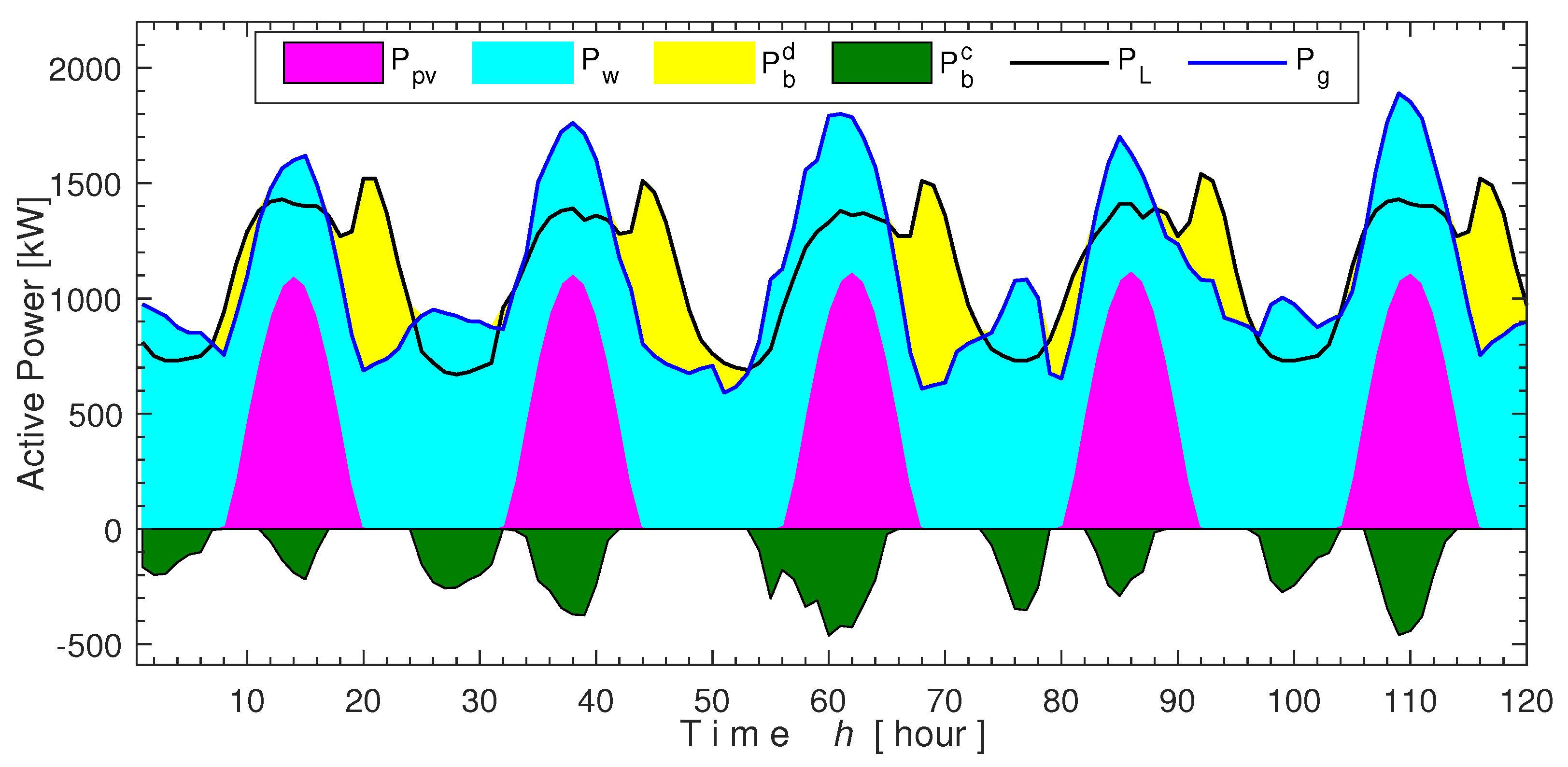
6.1. Case 1: Component Sizing and Operation Planning without Considering Demand Response

In this case, the demand response program was not considered when simulating and evaluating the microgrid component sizing and operation planning for the system under study. As a result, the load demand must be met by the power generation output of the PV and WT, and whatever deficit or surplus power remains in the system will be regulated by the BESS. This scenario is considered the system’s base case. The optimum component size of the simulation under various reliabilities (LPSP = 0%, 2.5%, and 5%) and all related costs are summarized in

Table 3. Optimum size of each system component, total annualized costs, and the percentage costs for each component under varying system reliabilities’ requirements for case 1.

LPSP	0%	2.5%	5.0%
PV capacity (kW)	1230	1260	1260
% cost of PV/TAC	16%	19%	20%
WT capacity (kW)	1970	1910	1880
% cost of WT/TAC	39%	42%	44%
BESS size (kWh)	6400	5000	4400
% cost of BESS/TAC	45%	39%	36%
DRP operation costs (USD/year)	0	0	0
ESD	13%	12%	12%
TAC (USD/year)	$5.17\times {10}^5$	$4.62\times {10}^5$	$4.37\times {10}^5$
% change of TAC		−11%	−15%

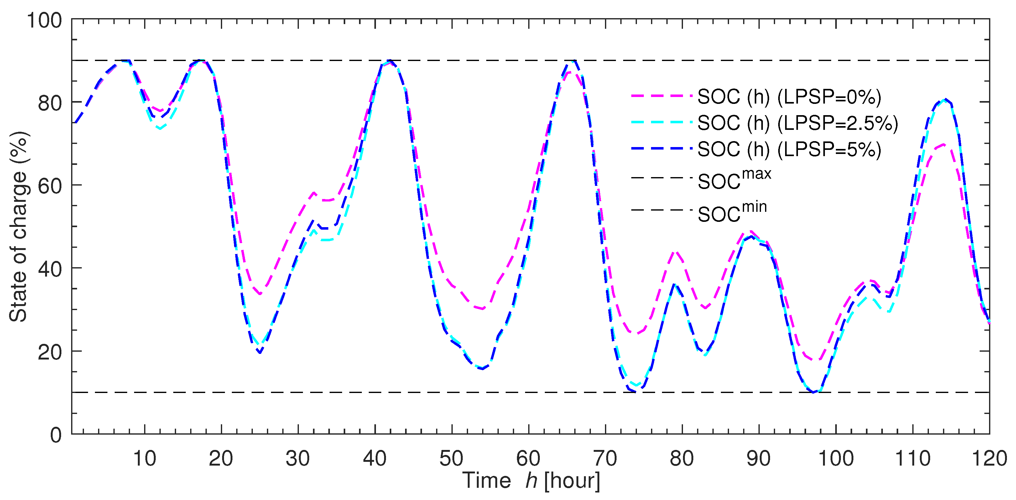
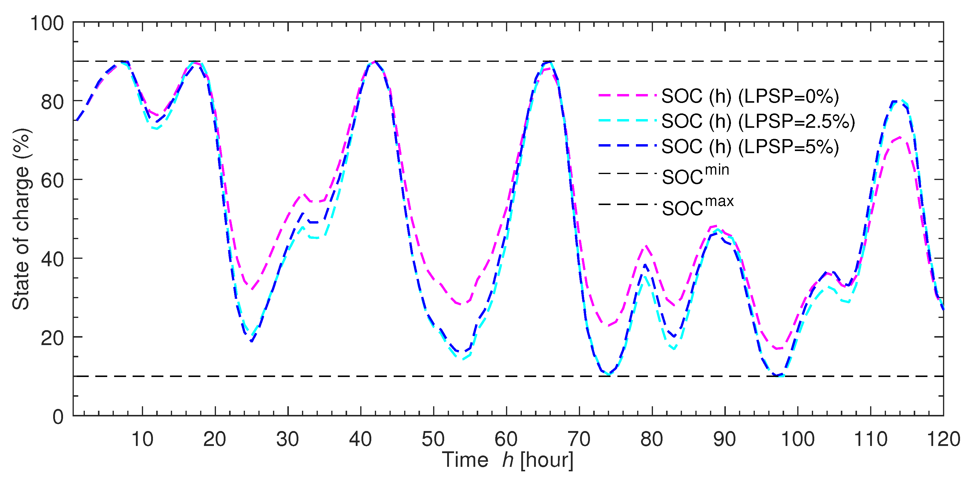
. Figure 3 shows the power dispatch of the various system units’ contribution to meet the load demand at the LPSP = 0%. Figure 4 compares the BESS utilization based on SOC at different levels of reliability (LPSP = 0%, 2.5%, and 5%).

The output power of the optimum system component sizes selected by the program can meet the load demand per the expected system requirements (LPSP = 0%), as shown in Figure 3. Since DRP is not considered, there are no costs related to the electricity market operation. As can be seen, there is a direct correlation between ESD, total yearly costs, reliability index, and system component size. Higher system reliability requirements necessitate larger PV, WT, and BESS system component sizes, increasing the total system cost (TAC). As per the results above, the BESS is the most expensive system component, which is about 45% of the total annualized costs of the microgrid due to the system’s higher dependency on ESS, as indicated by the high values of the ESD.

6.2. Case 2: VREs-Based Microgrid System’s Component Sizing and Operation Planning Considering CPP DRP

In this case, the potential benefit of CPP DRP on the capacity sizing and operation optimization for microgrids is explored. The system components’ sizes and costs are interrelated similar to case 1. The optimum component size of the simulation under various reliabilities (LPSP = 0%, 2.5%, and 5%) and all related costs are summarized in

Table 4. Techno-economic comparison and analysis of the system under study considering CPP DRP at various reliability levels for case 2.

LPSP	0%	2.5%	5.0%
PV capacity (kW)	1260	1290	1230
% cost of PV/TAC (USD/year)	17%	20%	19%
WT capacity (kW)	1960	1900	1880
% cost of WT/TAC (USD/year)	41%	44%	45%
BESS size (kWh)	5700	4500	4200
% cost of BESS/TAC (USD/year)	42%	37%	36%
DRP operation costs/TAC (%)	0%	0%	0%
ESD	12%	12%	11%
TAC (USD/year)	$4.92\times {10}^5$	$4.44\times {10}^5$	$4.28\times {10}^5$
% change of TAC		−10%	−13%

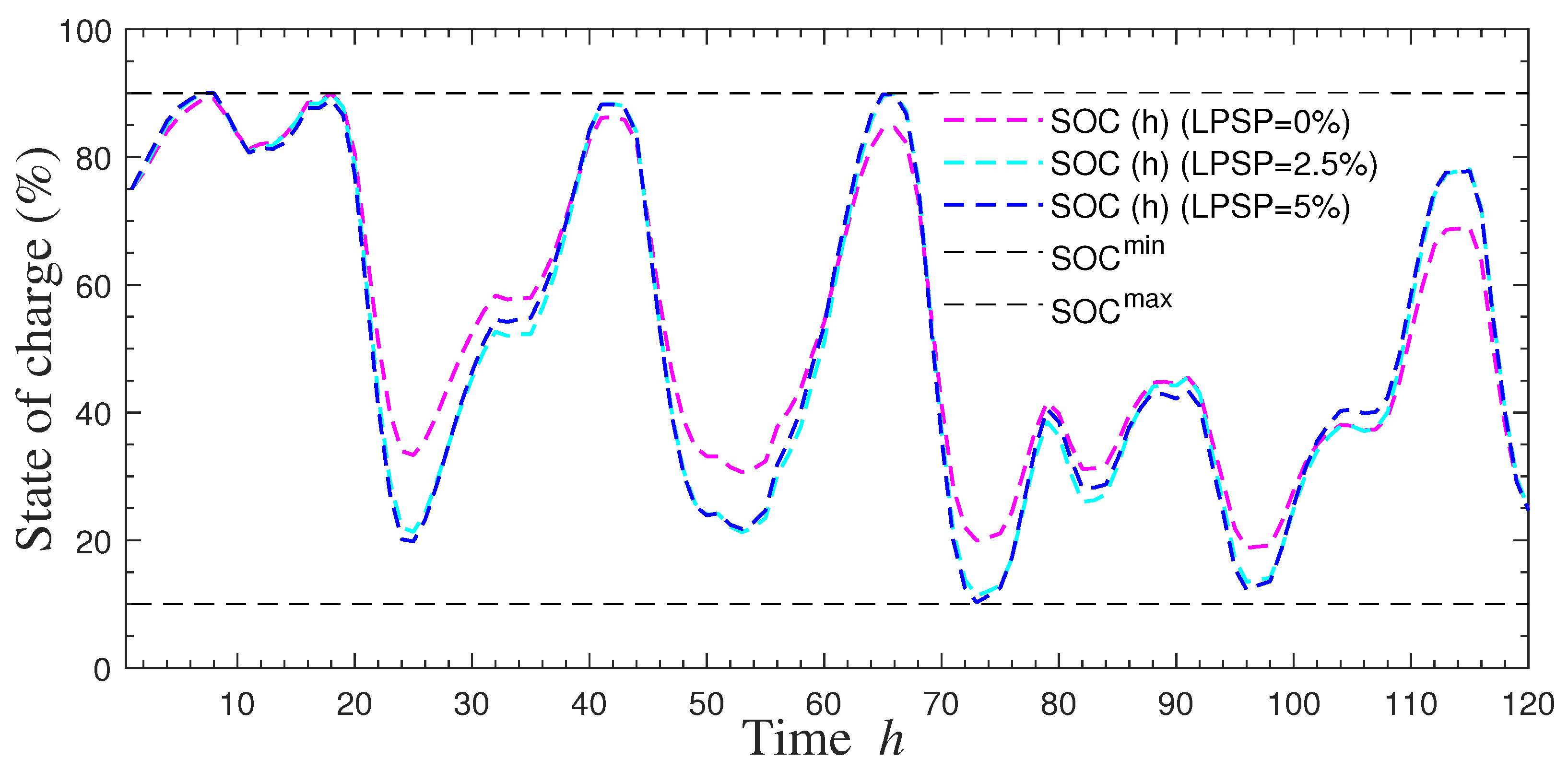
. Figure 5 shows the power dispatch of the various system units’ contributions to meet the load demand considering CPP DRP at the LPSP = 0%. Figure 6 compares the BESS utilization based on the state of charge at different levels of reliability (LPSP = 0%, 2.5%, and 5%).

The simulation results show that the higher the reliability requirements are for the system, the more expensive the system is, as depicted by the TAC values; this is because the reliability index (LPSP) and total system costs (TACs) have conflicting goals. Similarly, the more the system is dependent on ESS, the more expensive the system is; this is depicted by the higher percentage values of the ESD, which translates into higher costs for the BESS, as shown in Table 4.

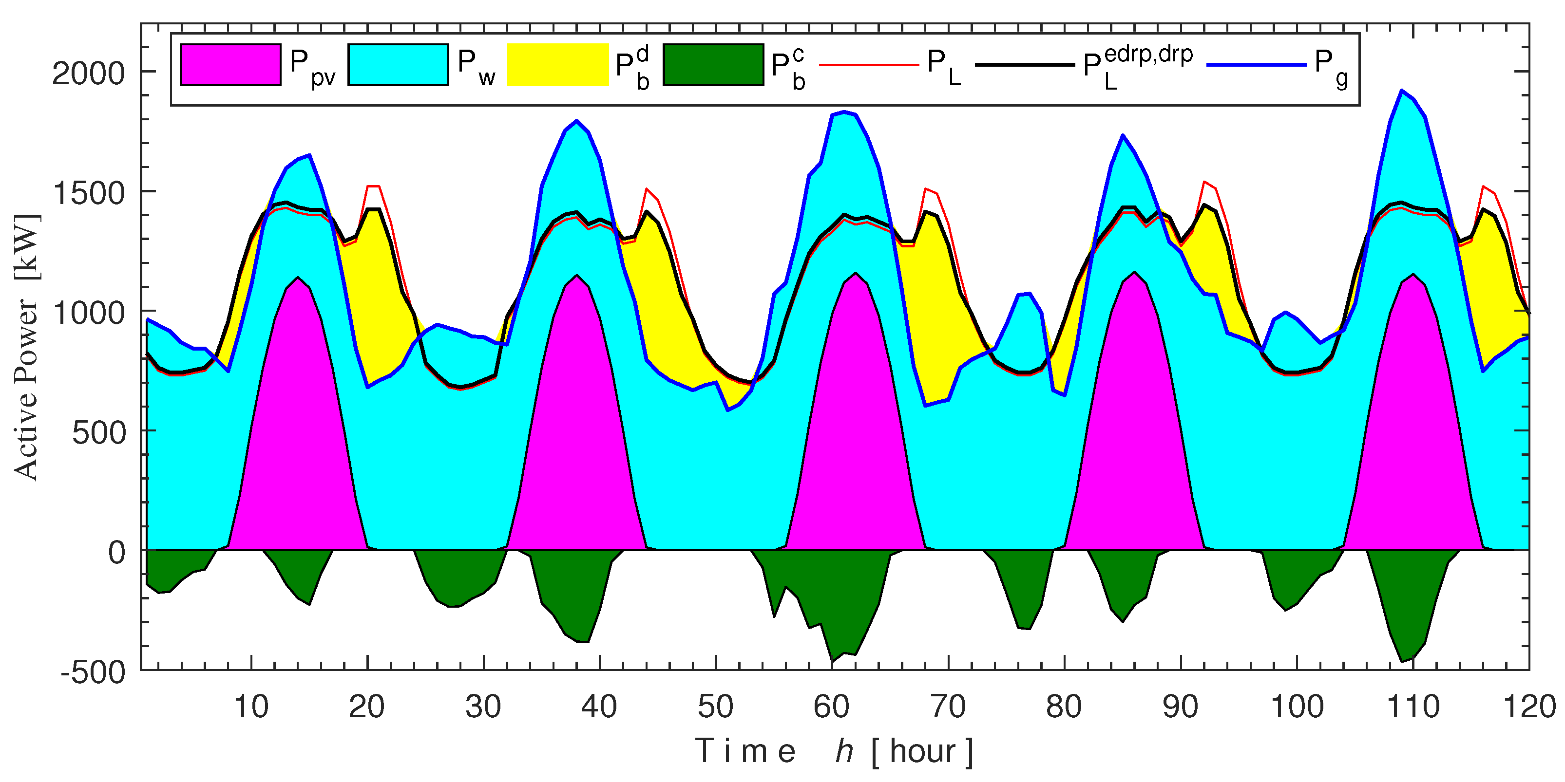
6.3. VREs-Based Microgrid System’s Component Sizing and Operation Planning Considering EDRP DRP

In this case, capacity sizing and operation planning are simulated and evaluated while considering EDRP at various reliability requirements.

Table 5. Techno-economic comparison and analysis of the system under study at various reliability levels for case 3 considering EDRP DRP.

LPSP	0%	2.5%	5.0%
PV capacity (kW)	1280	1300	1210
% cost of PV/TAC	17%	19%	19%
WT capacity (kW)	1950	1900	1890
% cost of WT/TAC	40%	43%	44%
BESS size (kWh)	5400	4300	4100
% cost of BESS/TAC	39%	34%	34%
DRP operation cost/TAC (%)	3.8%	3.7%	3.6%
ESD	11%	11%	12%
TAC (USD/year)	$5.00\times {10}^5$	$4.54\times {10}^5$	$4.39\times {10}^5$
% change of TAC		−9%	−12%

summarizes the system components’ sizes and related costs for the optimum microgrid configurations under varying reliability requirements (LPSP = 0%, 2.5%, and 5%). According to Table 5, unlike scenario 1 and 2, the total annualized costs (TACs) are composed of both expenses related to the equipment sizing and the operation strategy of the demand response program considered. In this case, the DRP operation costs are mainly due to incentive payments to customers participating in the EDRP program. Figure 7 shows the power output dispatch profile for the WT and PV and the BESS’s charging and discharging power. Figure 8 compares the BESS utilization at different levels of reliability (LPSP = 0%, 2.5%, and 5%) based on the state of charge.

6.4. VREs-Based Microgrid System’s Component Sizing and Operation Planning Considering PCDP DRP

This simulation scenario examines the potential benefits of the proposed PCDP DRP on capacity sizing and operation planning.

Table 6. Techno-economic comparison and analysis of the system under study considering PCDP DRP at various reliability levels for case 4.

LPSP	0%	2.5%	5.0%
PV capacity (kW)	1240	1220	1150
% cost of PV/TAC (USD/year)	18%	20%	19%
WT capacity (kW)	1990	1950	1920
% cost of WT/TAC (USD/year)	44%	47%	48%
BESS size (kWh)	4900	3900	3700
% cost of BESS/TAC (USD/year)	38%	33%	33%
ESD	10%	9%	9%
TAC (US USD/year)	$4.64\times {10}^5$	$4.22\times {10}^5$	$4.08\times {10}^5$
% change of TAC		−9%	−13%

summarizes the system components’ sizes and related costs for the optimum microgrid configurations under varying reliability requirements (LPSP = 0%, 2.5%, and 5%). The generation power output profile of the WT, PV, and BESS contribution in meeting the microgrid load demand is shown in Figure 9. Figure 10 compares the BESS utilization at different levels of reliability (LPSP = 0%, 2.5%, and 5%) based on the state of charge.

From the results, a relaxation of the system reliability requirement from 0% to 2.5% and 5% translates to a, respectively, 9% and 13% decrease in the total annualized costs (TACs); this is due to load reduction by the consumers during times of peak load demand and the power output of the generating units cannot meet the required capacity.

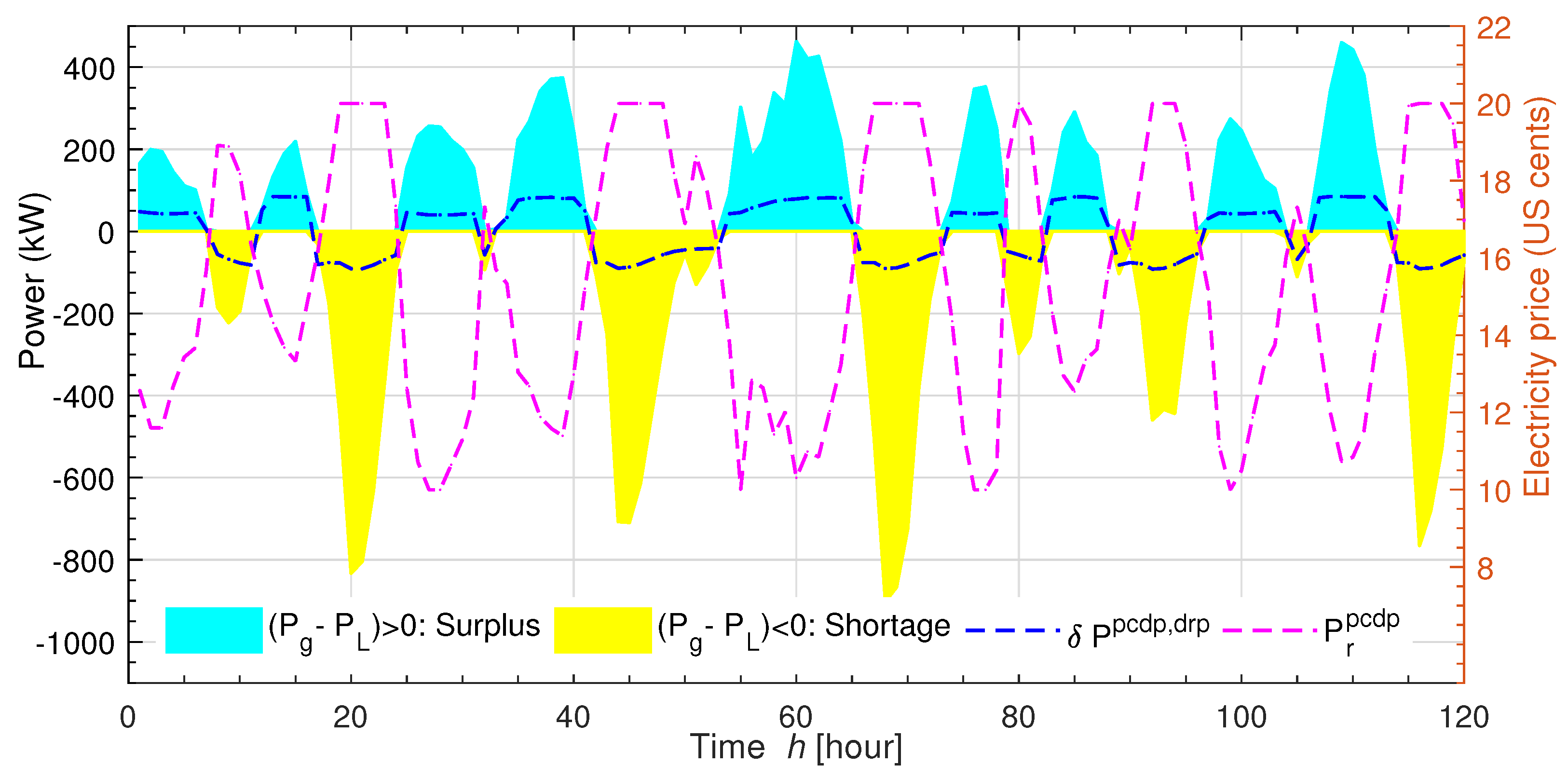
Furthermore, it is vital to note that the PCDP electricity pricing strategy is devised such that the flexible demand resources are shifted in such a way as to minimize both the shortage and surplus power in the system, thereby increasing the overall system efficiency. Consequently, the PCDP DRP techniques guarantee that the mismatch between the total output power of the VREs and the load demand is minimized; thus, the ESD is minimum in all cases, resulting in a significant reduction in the BESS capacity requirement. Figure 11 shows the new electricity price versus the power mismatch in the system due to the impact of PCDP DRP program implementation.

6.5. Techno-Economic Comparison for Each of the Scenarios Based on Demand Response Program Options at Maximum System Reliability (LPSP = 0%)

The techno-economic benefits of each DRP in the long-term investment and short-term microgrid planning for the proposed VREs-based system are assessed and analyzed in this section for the four cases considered. The techno-economic comparison for each of the cases based on DRP options at maximum system reliability (LPSP = 0%) is summarized in

Table 7. Techno-economic comparison for each scenario based on demand response program options at maximum system reliability (LPSP = 0%).

Case	Case 1	Case 2	Case 3	Case 4
Type of DRP	None	CPP DRP	EDRP DRP	PCDP DRP
PV capacity (kW)	1230	1260	1280	1240
% change of PV	-	2%	4%	1%
WT capacity (kW)	1970	1960	1950	1990
% change of WT	-	−1%	−1%	1%
BESS capacity (kW)	6400	5700	5400	4900
% change in BESS	-	−11%	−16%	−23%
Total energy consumed (kWh/year)	$9.91\times {10}^6$	$9.91\times {10}^6$	$9.91\times {10}^6$	$9.91\times {10}^6$
Load curtailed (kWh/year)	0%	−0.027%	−0.024%	0%
Total cost of energy (USD/year)	$1.57\times {10}^8$	$1.56\times {10}^8$	$1.57\times {10}^8$	$1.53\times {10}^8$
DRP Operation Cost/TAC (%)	0.0%	0.0%	3.8%	0.0%
ESD(%)	13%	12%	11%	10%
Total annualized costs (USD/year)	$5.17\times {10}^5$	$4.92\times {10}^5$	$5.00\times {10}^5$	$4.64\times {10}^5$
% change of TAC	-	−5%	−3%	−10%

.

Case 1 is the most expensive system compared to all four cases, with a total annualized cost of USD $5.17\times {10}^5$/year. Since there is no inclusion of demand-side management in this case and the VREs’ power output cannot be dispatched or controlled, the battery energy is the only flexible resource depended upon to address the mismatch between the generation and the load demand. Thus, a BESS capacity of approximately 6400 kWh is needed to serve the load demand as per the set reliability requirement, consequently, a high ESD value of about 13%. It is worth noting that the BESS is the most expensive component amounting to about 45% of the TAC; thus, the need for DRP to lessen the reliance of the BESS in the system. Considering the DRP in case 2, the benefit of the CPP DRP results in a cost saving of approximately 5% of the total annualized costs compared to the reference case, from US $5.17\times {10}^5$ (without DRP) to $4.92\times {10}^5$ (with CPP DRP considered).

The cost reduction, in this case, is attributed to a drop in ESD requirement from 13% to 12%. Since the CPP DRP reduces the load demand from the maximum peak load periods to off-peak periods, thus, a lower BESS size is required. Consequently, a BESS capacity of 5700 kWh is sufficient to meet the load demand per set system reliability, which is about a 10% decrease in BESS size compared to the reference case. However, implementing the CPP DRP results in a load curtailment of about 0.027% of the total load demand by the consumers. This is because the CPP DRP penalizes the electricity consumers by enforcing high pricing during peak periods; the electricity consumers are therefore compelled to curtail or minimize their power consumption due to cutting down electricity costs, which is an undesirable effect.

Compared to the reference case (case 1), the implementation of EDRP in case 3 has various cost–benefits to long-term investment planning, as shown in Table 7. The resulting load profile, due to the EDRP DRP adoption, yields a 2% decrease in ESD from 13% to 11% as the FDRs are being shifted from the high peak period with high ESS dependencies to the low peak period where there are surplus generations from the VREs; this results in a 3% decrease in the TAC compared to case 1. It is worth noting that compared to the previous case of CPP DRP, the TAC is slightly higher due to the cost of running the EDRP electricity market strategy, as the system operators have to pay consumers some incentives for complying with the requirement to reduce energy consumption during EDRP peak load periods. Furthermore, it could be observed that EDRP also results in a 0.024% reduction in the overall load demand, which is also an undesired consequence.

The techno-economic aspect of PCDR DRP is noted to significantly impact both long-term investment and operational planning. From the electricity consumer side, the DRP participating clients have a cost savings of about 2.54% for an equal amount of consumed energy compared to the reference case (case 1); since PCDP DRP gives the most considerable cost saving compared to the two other cases (case 3 with EDRP and case 2 with CPP) and the aggregate energy consumption equals the total demand of the base case, meaning that there is no load demand curtailment; thus, this is the most preferred demand response program. As a result of implementing the DPCP pricing scheme, consumers have sufficient motivation to shift their load demand profile from high electricity price periods to low price periods, thereby fetching the lowest prices; thus, the overall cost saving compared to the three other cases.

From a generation planning perspective, deploying the PCDP DRP program yields a new load profile optimal for the day-to-day operation and long-term investment planning. As the PCDP pricing scheme encourages consumers to time shift the FDRs from peak load periods to coincide with peak periods of VREs generation, the system dependency on the ESS is drastically reduced, thus resulting in a lower value of ESD of about 9%. Therefore, the capacity of the BESS needed to balance the power mismatch in the system is significantly reduced by 23%, and thus, the TAC is also reduced by 10%. 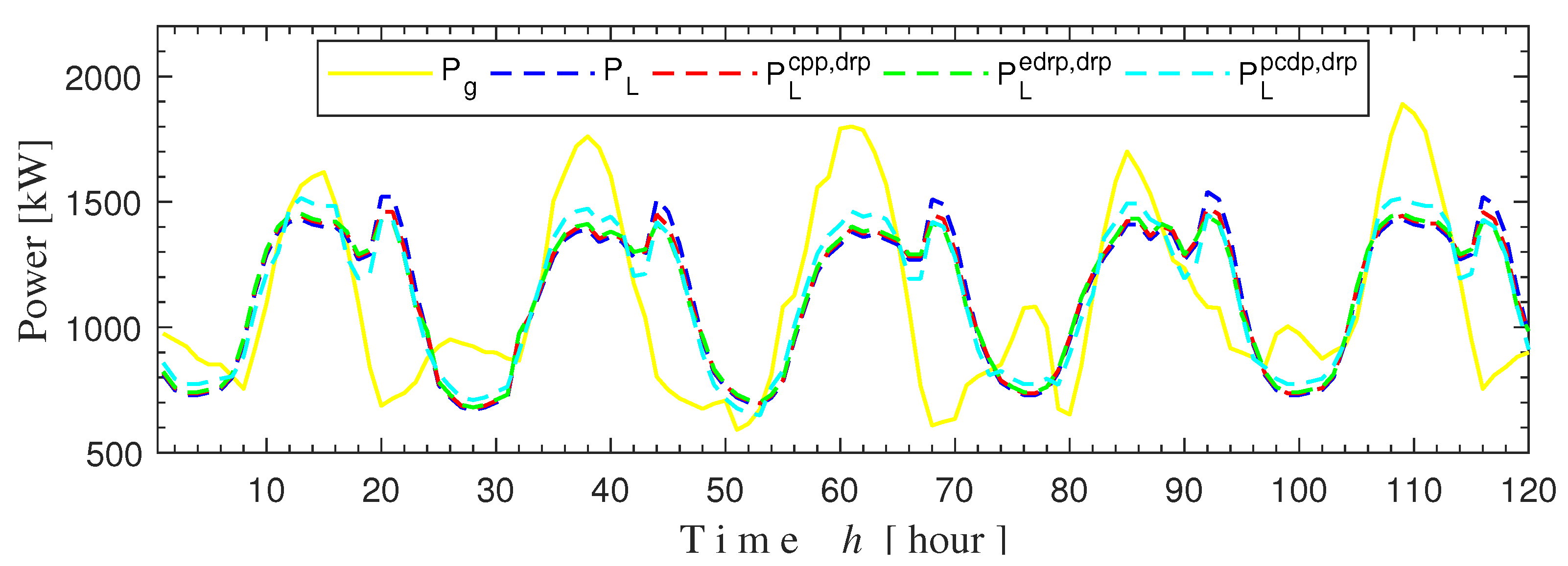Figure 12 demonstrates and compares the impacts of DRPs in decreasing the mismatch between the surplus and shortage of power in the system due to the variability of VREs generated power and load demand.

7. Conclusions

This paper proposed a joint bi-optimization planning approach for merging capacity sizing and operation planning into a single model, with and without considering DRPs, while maximizing the loss of power probability to realize a practicable VREs-based microgrid system. The primary objective is to determine the optimum size of the PV, WT, and BESS, and the most suitable operative schedules to achieve an ideal operating strategy that maximizes the designed components’ installed capacity and minimizes the total annualized costs while maximizing the LSPS. An improved PCDP DRP with a dynamic pricing technique devised to schedule FDR based on the system’s surplus and deficit power imbalances at any given time is proposed and investigated. The proposed PCDP is contrasted against the classical EDRP and CPP DRP to validate its robustness and potential benefits. Additionally, this work has proposed and validated a quantitative metric for evaluating the designed energy storage capacity’s performances. Four simulation cases were explored and solved using the epsilon constraint mixed-integer linear programming algorithm on the MATLAB environment to ascertain the prospects of incorporating DRPs in VREs-based microgrid planning and validate the proposed methodology’s potential benefits. The e-constraint MILP optimization was selected based on its proven superior capability of producing a credible and dependable solution with minimal computation time and reduced modeling complexities. From the results, the cost-benefit advantage of each DRP is verified to improve the system’s overall performance, and minimizing the total annualized costs is undoubtedly exemplified. Moreover, the PCDP DRP is confirmed to have superior cost-benefits in reducing the system costs compared to other DRPs due to its ability to match the peak surplus power generation with the maximum attainable capacity of FDRs and vice versa. Thus, from the findings of this work, the proposed planning approach incorporating PCDP DRP indicates that the proposed methodology is practicable, viable, and efficient in determining the most cost-effective planning approach for a grid-independent VREs-based microgrid system.

References

1. Bonilla, J.; Blanco, J.; Zarza, E.; Alarcón-Padilla, D.C. Feasibility and practical limits of full decarbonization of the electricity market with renewable energy: Application to the Spanish power sector. Energy 2022, 239, 122437. [Google Scholar] [CrossRef]
2. Kiptoo, M.K.; Adewuyi, O.B.; Lotfy, M.E.; Amara, T.; Konneh, K.V.; Senjyu, T. Assessing the techno-economic benefits of flexible demand resources scheduling for renewable energy–based smart microgrid planning. Future Internet 2019, 11, 219. [Google Scholar] [CrossRef]
3. Dalala, Z.; Al-Omari, M.; Al-Addous, M.; Bdour, M.; Al-Khasawneh, Y.; Alkasrawi, M. Increased renewable energy penetration in national electrical grids constraints and solutions. Energy 2022, 246, 123361. [Google Scholar] [CrossRef]
4. Groppi, D.; Pfeifer, A.; Garcia, D.A.; Krajačić, G.; Duić, N. A review on energy storage and demand side management solutions in smart energy islands. Renew. Sustain. Energy Rev. 2021, 135, 110183. [Google Scholar] [CrossRef]
5. Impram, S.; Nese, S.V.; Oral, B. Challenges of renewable energy penetration on power system flexibility: A survey. Energy Strategy Rev. 2020, 31, 100539. [Google Scholar] [CrossRef]
6. Shoferpour, A.; Karimi, A. Improving the flexibility of power systems using transportable battery, transmission switching, demand response, and flexible ramping product market in the presence of high wind power. IET Renew. Power Gener. 2023, 17, 1413–1435. [Google Scholar] [CrossRef]
7. Yang, X.; Chai, G.; Liu, X.; Xu, M.; Guo, Q. Storage-Transmission Joint Planning Method to Deal with Insufficient Flexibility and Transmission Congestion. Front. Energy Res. 2021, 8, 612909. [Google Scholar] [CrossRef]
8. Alexopoulos, D.K.; Anastasiadis, A.G.; Vokas, G.A.; Kaminaris, S.D.; Psomopoulos, C.S. A review of flexibility options for high RES penetration in power systems—Focusing the Greek case. Energy Rep. 2021, 7, 33–50. [Google Scholar] [CrossRef]
9. Babatunde, O.M.; Munda, J.L.; Hamam, Y. Power system flexibility: A review. Energy Rep. 2020, 6, 101–106. [Google Scholar] [CrossRef]
10. Gelazanskas, L.; Gamage, K.A. Demand side management in smart grid: A review and proposals for future direction. Sustain. Cities Soc. 2014, 11, 22–30. [Google Scholar] [CrossRef]
11. Davito, B.; Tai, H.; Uhlaner, R. The smart grid and the promise of demand-side management. McKinsey Smart Grid 2010, 3, 8–44. [Google Scholar]
12. Mohammad, N.; Mishra, Y. Demand-side management and demand response for smart grid. In Smart Grids and Their Communication Systems; Springer: Singapore, 2019; pp. 197–231. [Google Scholar]
13. Nwulu, N.I.; Xia, X. Optimal dispatch for a microgrid incorporating renewables and demand response. Renew. Energy 2017, 101, 16–28. [Google Scholar] [CrossRef]
14. Shang, N.; Lin, Y.; Ding, Y.; Ye, C.; Yan, J. Nodal market power assessment of flexible demand resources. Appl. Energy 2019, 235, 564–577. [Google Scholar] [CrossRef]
15. Vahid-Ghavidel, M.; Javadi, M.S.; Gough, M.; Santos, S.F.; Shafie-Khah, M.; Catalao, J.P.S. Demand response programs in multi-energy systems: A review. Energies 2020, 13, 4332. [Google Scholar] [CrossRef]
16. Kiptoo, M.K.; Adewuyi, O.B.; Lotfy, M.E.; Senjyu, T.; Mandal, P.; Abdel-Akher, M. Multi-objective optimal capacity planning for 100% renewable energy-based microgrid incorporating cost of demand-side flexibility management. Appl. Sci. 2019, 9, 3855. [Google Scholar] [CrossRef]
17. Zeng, B.; Liu, Y.; Xu, F.; Liu, Y.; Sun, X.; Ye, X. Optimal demand response resource exploitation for efficient accommodation of renewable energy sources in multi-energy systems considering correlated uncertainties. J. Clean. Prod. 2021, 288, 125666. [Google Scholar] [CrossRef]
18. Olawuyi, N.; Akorede, M.; Femi, E.; Ayeni, A.; Jimoh, R. Real-time demand response algorithm for minimising industrial consumers electricity billing. In Proceedings of the 2017 IEEE 3rd International Conference on Electro-Technology for National Development (NIGERCON), Owerri, Nigeria, 7–10 November 2017; pp. 1061–1066. [Google Scholar]
19. Muratori, M.; Rizzoni, G. Residential Demand Response: Dynamic Energy Management and Time-Varying Electricity Pricing. IEEE Trans. Power Syst. 2016, 31, 1108–1117. [Google Scholar] [CrossRef]
20. Moghimi, F.H.; Barforoushi, T. A short-term decision-making model for a price-maker distribution company in wholesale and retail electricity markets considering demand response and real-time pricing. Int. J. Electr. Power Energy Syst. 2020, 117, 105701. [Google Scholar] [CrossRef]
21. McPherson, M.; Stoll, B. Demand response for variable renewable energy integration: A proposed approach and its impacts. Energy 2020, 197, 117205. [Google Scholar] [CrossRef]
22. Gomes, P.V.; Saraiva, J.T. State-of-the-art of transmission expansion planning: A survey from restructuring to renewable and distributed electricity markets. Int. J. Electr. Power Energy Syst. 2019, 111, 411–424. [Google Scholar] [CrossRef]
23. Heidari Yazdi, S.S.; Rahimi, T.; Khadem Haghighian, S.; Gharehpetian, G.B.; Bagheri, M. Over-voltage regulation of distribution networks by coordinated operation of PV inverters and demand side management program. Front. Energy Res. 2022, 10, 920654. [Google Scholar] [CrossRef]
24. Wyrwa, A.; Suwała, W.; Pluta, M.; Raczyński, M.; Zyśk, J.; Tokarski, S. A new approach for coupling the short-and long-term planning models to design a pathway to carbon neutrality in a coal-based power system. Energy 2022, 239, 122438. [Google Scholar] [CrossRef]
25. Prina, M.G.; Lionetti, M.; Manzolini, G.; Sparber, W.; Moser, D. Transition pathways optimization methodology through EnergyPLAN software for long-term energy planning. Appl. Energy 2019, 235, 356–368. [Google Scholar] [CrossRef]
26. Kaluthanthrige, R.; Rajapakse, A.D. Demand response integrated day-ahead energy management strategy for remote off-grid hybrid renewable energy systems. Int. J. Electr. Power Energy Syst. 2021, 129, 106731. [Google Scholar] [CrossRef]
27. Pang, Y.; Pan, L.; Zhang, J.; Chen, J.; Dong, Y.; Sun, H. Integrated sizing and scheduling of an off-grid integrated energy system for an isolated renewable energy hydrogen refueling station. Appl. Energy 2022, 323, 119573. [Google Scholar] [CrossRef]
28. Xiang, Y.; Cai, H.; Gu, C.; Shen, X. Cost-benefit analysis of integrated energy system planning considering demand response. Energy 2020, 192, 116632. [Google Scholar] [CrossRef]
29. Wang, X.; Palazoglu, A.; El-Farra, N.H. Operational optimization and demand response of hybrid renewable energy systems. Appl. Energy 2015, 143, 324–335. [Google Scholar] [CrossRef]
30. Das, P.; Mathur, J.; Bhakar, R.; Kanudia, A. Implications of short-term renewable energy resource intermittency in long-term power system planning. Energy Strategy Rev. 2018, 22, 1–15. [Google Scholar] [CrossRef]
31. Gebremeskel, D.H.; Ahlgren, E.O.; Beyene, G.B. Long-term electricity supply modelling in the context of developing countries: The OSeMOSYS-LEAP soft-linking approach for Ethiopia. Energy Strategy Rev. 2023, 45, 101045. [Google Scholar] [CrossRef]
32. Mohseni, S.; Brent, A.C.; Kelly, S.; Browne, W.N. Demand response-integrated investment and operational planning of renewable and sustainable energy systems considering forecast uncertainties: A systematic review. Renew. Sustain. Energy Rev. 2022, 158, 112095. [Google Scholar] [CrossRef]
33. Mina-Casaran, J.D.; Echeverry, D.F.; Lozano, C.A. Demand response integration in microgrid planning as a strategy for energy transition in power systems. IET Renew. Power Gener. 2021, 15, 889–902. [Google Scholar] [CrossRef]
34. Kiptoo, M.K.; Lotfy, M.E.; Adewuyi, O.B.; Conteh, A.; Howlader, A.M.; Senjyu, T. Integrated approach for optimal techno-economic planning for high renewable energy-based isolated microgrid considering cost of energy storage and demand response strategies. Energy Convers. Manag. 2020, 215, 112917. [Google Scholar] [CrossRef]
35. Shariatzadeh, F.; Mandal, P.; Srivastava, A.K. Demand response for sustainable energy systems: A review, application and implementation strategy. Renew. Sustain. Energy Rev. 2015, 45, 343–350. [Google Scholar] [CrossRef]
36. Kharrich, M.; Akherraz, M.; Sayouti, Y. Optimal sizing and cost of a Microgrid based in PV, WIND and BESS for a School of Engineering. In Proceedings of the 2017 International Conference on Wireless Technologies, Embedded and Intelligent Systems (WITS), Fez, Morocco, 19–20 April 2017; pp. 1–5. [Google Scholar]
37. Yousefi, S.; Moghaddam, M.P.; Majd, V.J. Optimal real time pricing in an agent-based retail market using a comprehensive demand response model. Energy 2011, 36, 5716–5727. [Google Scholar] [CrossRef]
38. Ning, J.; Peng, Q.; Zhu, Y.; Jiang, Y.; Nielsen, O.A. A Bi-objective optimization model for the last train timetabling problem. J. Rail Transp. Plan. Manag. 2022, 23, 100333. [Google Scholar] [CrossRef]
39. Fodhil, F.; Hamidat, A.; Nadjemi, O. Potential, optimization and sensitivity analysis of photovoltaic-diesel-battery hybrid energy system for rural electrification in Algeria. Energy 2019, 169, 613–624. [Google Scholar] [CrossRef]
40. Javanmard, M.E.; Ghaderi, S.; Sangari, M.S. Economic and Environmental Analysis of nZEB model with smartification building using MILP. In Proceedings of the 2020 IEEE International Conference on Environment and Electrical Engineering and 2020 IEEE Industrial and Commercial Power Systems Europe (EEEIC/I&CPS Europe), Madrid, Spain, 9–12 June 2020; pp. 1–6. [Google Scholar]
41. Yuan, Z.; Wang, W.; Li, J. Carbon dioxide recycling in hydrogen-based energy systems using power-to-gas facility and stochastic multi-objective optimization. J. Clean. Prod. 2023, 387, 135892. [Google Scholar] [CrossRef]
42. Akter, H.; Howlader, H.O.R.; Saber, A.Y.; Mandal, P.; Takahashi, H.; Senjyu, T. Optimal sizing of hybrid microgrid in a remote island considering advanced direct load control for demand response and low carbon emission. Energies 2021, 14, 7599. [Google Scholar] [CrossRef]
43. The Presidency, Republic of Kenya. Power Generation and Transmission Master Plan, Kenya Medium Term Plan 2015–2020 Volume I; 2016. Available online: https://www.erc.go.ke/ (accessed on 1 April 2019).
44. Weather Mount Marsabit. 2019. Available online: https://www.meteoblue.com/en/weather/forecast/week/mount-marsabit_kenya_187584 (accessed on 1 April 2019).
45. Photovoltaic Geographical Information System. 2019. Available online: https://rem.jrc.ec.europa.eu (accessed on 1 April 2019).
46. Ministry of Energy and Petroleum, Republic of Kenya. Updated Least Cost Power Development Plan 2017–2037. 2018. Available online: http://www.decoalonize.org/wp-content/uploads/2019/09/LCPDP-Least-Cost-Power-Development-Plan-2017-2037-not-2022-updated-June-2018.pdf (accessed on 1 November 2022).
47. Kairies, K.P. Battery Storage Technology Improvements and Cost Reductions to 2030: A Deep Dive; IRENA: Abu Dhabi, United Arab Emirates, 2017. [Google Scholar]
48. Jaiswal, A. Lithium-ion battery based renewable energy solution for off-grid electricity: A techno-economic analysis. Renew. Sustain. Energy Rev. 2017, 72, 922–934. [Google Scholar] [CrossRef]
49. Dhundhara, S.; Verma, Y.P.; Williams, A. Techno-economic analysis of the lithium-ion and lead-acid battery in microgrid systems. Energy Convers. Manag. 2018, 177, 122–142. [Google Scholar] [CrossRef]
50. Aalami, H.; Moghaddam, M.P.; Yousefi, G. Demand response modeling considering interruptible/curtailable loads and capacity market programs. Appl. Energy 2010, 87, 243–250. [Google Scholar] [CrossRef]
51. Tarrif Setting: Electricity. 2019. Available online: https://www.erc.go.ke/services/economic-regulation/tarrif-setting/tarrif-setting-electricity/ (accessed on 1 April 2019).
52. Electricity Cost Tariffs & Schedule of Tariffs 2018. 2019. Available online: http://kplc.co.ke/content/item/691/electricity-cost-tariffs—schedule-of-tariffs-2018 (accessed on 1 April 2019).
53. Aalami, H.; Moghaddam, M.P.; Yousefi, G. Modeling and prioritizing demand response programs in power markets. Electr. Power Syst. Res. 2010, 80, 426–435. [Google Scholar] [CrossRef]
54. Khezri, R.; Mahmoudi, A. Review on the state-of-the-art multi-objective optimisation of hybrid standalone/grid-connected energy systems. IET Gener. Transm. Distrib. 2020, 14, 4285–4300. [Google Scholar] [CrossRef]
55. Nguyen, T.H.T.; Nakayama, T.; Ishida, M. Optimal capacity design of battery and hydrogen system for the DC grid with photovoltaic power generation based on the rapid estimation of grid dependency. Int. J. Electr. Power Energy Syst. 2017, 89, 27–39. [Google Scholar] [CrossRef]
56. Airò Farulla, G.; Tumminia, G.; Sergi, F.; Aloisio, D.; Cellura, M.; Antonucci, V.; Ferraro, M. A review of key performance indicators for building flexibility quantification to support the clean energy transition. Energies 2021, 14, 5676. [Google Scholar] [CrossRef]
Figure 1. Proposed system configuration model.
Energies 16 04147 g001
Figure 2. The flowchart for the microgrid planning with demand-side management.
Energies 16 04147 g002
Figure 3. Power dispatch profile of the various system units’ contribution to meeting the load demand at the LPSP = 0% (Case 1).
Energies 16 04147 g003
Figure 4. A comparison of the BESS utilization based on the state of charge at different levels of reliability requirements (LPSP = 0%, 2.5%, and 5%).
Energies 16 04147 g004
Figure 5. A comparison of the BESS utilization at different levels of reliability (LPSP = 0%, 2.5%, and 5%) based on the state of charge (case 2).
Energies 16 04147 g005
Figure 6. Power dispatch profile of the various system units’ contributions to meet the load demand considering CPP DRP at the LPSP = 0% (Case 2).
Energies 16 04147 g006
Figure 7. Power output dispatch profile for the WT and PV and the BESS’s charging and discharging power (Case 3).
Energies 16 04147 g007
Figure 8. A comparison of the BESS utilization at different levels of reliability (LPSP = 0%, 2.5%, and 5%) based on the state of charge (case 3).
Energies 16 04147 g008
Figure 9. Shows the power output dispatch profile for the WT and PV and BESS’s charging and discharging power at LPSP = 0% (Case 4).
Energies 16 04147 g009
Figure 10. A comparison of the BESS utilization based at different levels of reliability (LPSP = 0%, 2.5%, and 5%) on the state of charge (Case 4).
Energies 16 04147 g010
Figure 11. The new electricity price versus the power output mismatch in the system due to the impact of PCDP DRP program implementation.
Energies 16 04147 g011
Figure 12. A comparison of the impacts of DRPs in decreasing the mismatch between the surplus and shortage power in the system due to the variability of VREs-generated power and load demand.
Energies 16 04147 g012